A note on the optimal degree of the weak gradient of the stabilizer free weak Galerkin finite element method

Abstract

Recently, a new stabilizer free weak Galerkin method (SFWG) is proposed, which is easier to implement. The idea is to raise the degree of polynomials $j$ for computing weak gradient. It is shown that if $j\geq j_{0}$ for some $j_{0}$, then SFWG achieves the optimal rate of convergence. However, large $j$ will cause some numerical difficulties. To improve the efficiency of SFWG and avoid numerical locking, in this note, we provide the optimal $j_{0}$ with rigorous mathematical proof.

1 Introduction

In this note, similar to [1], we will consider the following Poisson equation

(1) $$-\Delta u = f\quad\mbox{ in }\Omega,$$

(2) $$u = 0\quad\mbox{ on }\partial\Omega,$$

as the model problem, where $\Omega$ is a polygonal domain in $\mathbb{R}^{2}$. The variational formulation of the Poisson problem (1)-(2) is to seek $u\in H_{0}^{1}(\Omega)$ such that

(3) $$(\nabla u,\nabla v) = (f,v),\qquad\forall v\in H_{0}^{1}(\Omega).$$

A stabilizer free weak Galerkin finite element method is proposed by Ye and Zhang in [1] as a new method for the solution of Poisson equation on polytopal meshes in 2D or 3D. Let $j$ be the degree of polynomials for the calculation of weak gradient. It has been proved in [1] that there is a $j_{0}>0$ so that the SFWG method converges with optimal order of convergence for any $j\geq j_{0}$. However, when $j$ is too large, the magnitude of the weak gradient can be extremely large, causing numerical instability. In this note, we provide the optimal $j_{0}$ to improve the efficiency and avoid unnecessary numerical difficulties, which has mathematical and practical interests.

2 Weak Galerkin Finite Element Schemes

Let ${\cal T}_{h}$ be a partition of the domain $\Omega$ consisting of polygons in 2D. Suppose that ${\cal T}_{h}$ is shape regular in the sense defined by (2.7)-(2.8) and each $T$ is convex. Let ${\cal E}_{h}$ be the set of all edges in ${\cal T}_{h}$, and let ${\cal E}_{h}^{0}={\cal E}_{h}\setminus\partial\Omega$ be the set of all interior edges. For each element $T\in{\cal T}_{h}$, denote by $h_{T}$ the diameter of $T$, and $h=max_{T\in{\cal T}_{h}}h_{T}$ the mesh size of ${\cal T}_{h}$.

On $T$, let $P_{k}(T)$ be the space of all polynomials with degree no greater than $k$. Let $V_{h}$ be the weak Galerkin finite element space associated with $T\in{\cal T}_{h}$ defined as follows:

(4) $$V_{h} = \{v=\{v_{0},v_{b}\}:v_{0}|_{T}\in P_{k}(T),v_{b}|_{e}\in P_{k}(e),e\in\partial T,T\in{\cal T}_{h}\},$$

where $k\geq 1$ is a given integer. In this instance, the component $v_{0}$ symbolizes the interior value of $v$, and the component $v_{b}$ symbolizes the edge value of $v$ on each $T$ and $e$, respectively. Let $V^{0}_{h}$ be the subspace of $V_{h}$ defined as:

(5) $$V_{h}^{0} = \{v:v\in V_{h},v_{b}=0\mbox{ on }\partial\Omega\}.$$

For any $v=\{v_{0},v_{b}\}\in V_{h}+H^{1}(\Omega),$ the weak gradient $\nabla_{w}v\in[P_{j}(T)]^{2}$ is defined on $T$ as the unique polynomial satisfying

(6) $$(\nabla_{w}v,\mathbf{q})_{T} = -(v_{0},\mathbf{\nabla\cdot q})_{T}+\langle v_{b},\mathbf{q\cdot\mathbf{n}}\rangle_{\partial T},\quad\forall\mathbf{q}\in[P_{j}(T)]^{2},j\geq k.$$

where $\mathbf{n}$ is the unit outward normal vector of $\partial T$.

For simplicity, we adopt the following notations,

$$(v,w)_{{\cal T}_{h}}=\sum_{T\in{\cal T}_{h}}(v,w)_{T}=\sum_{T\in{\cal T}_{h}}\int_{T}vwdx,$$

$$\left\langle v,w\right\rangle_{\partial{\cal T}_{h}}=\sum_{T\in{\cal T}_{h}}\left\langle v,w\right\rangle_{\partial T}=\sum_{T\in{\cal T}_{h}}\int_{\partial T}vwdx.$$

For any $v=\left\{v_{0},v_{b}\right\}$ and $w=\left\{w_{0},w_{b}\right\}$ in $V_{h}$, we define the bilinear forms as follows:

(7) $$A(v,w) =\sum_{T\in{\cal T}_{h}}(\nabla_{w}v,\nabla_{w}w)_{T}.$$

Stabilizer free Weak Galerkin Algorithm 1.

A numerical solution for (1)-(2) can be obtain by finding $u_{h}=\{v_{0},v_{b}\}\in V_{h}^{0}$, such that the following equation holds

(8) $$A(u_{h},v)=(f,v_{0}),\quad\forall v=\{v_{0},v_{b}\}\in V_{h}^{0}.$$

where $A(\cdot,\cdot)$ is defined in (7).

Accordingly, for any $v\in V_{h}^{0}$, we define an energy norm ${|||}\cdot{|||}$ on $V_{h}^{0}$ as:

(9) $${|||}v{|||}^{2}=\sum_{T\in{\cal T}_{h}}(\nabla_{w}v,\nabla_{w}v)_{T}=\sum_{T\in{\cal T}_{h}}\|\nabla_{w}v\|^{2}_{T}.$$

An $H^{1}$ norm on $V_{h}^{0}$ is defined as:

$$\|v\|_{1,h}^{2}=\sum_{T\in{\cal T}_{h}}\left(\|\nabla v_{0}\|^{2}_{T}+h_{T}^{-1}\|v_{0}-v_{b}\|^{2}_{\partial T}\right).$$

The following well known lemma and corollary will be needed in proving our main result.

Lemma 1.

Suppose that $D_{1}\subset D_{2}$ are convex regions in $\mathbb{R}^{d}$ such that $D_{2}$ can be obtain by scaling $D_{1}$ with a factor $r>1$. Then for any $p\in P_{n}(D_{2})$,

$$\|p\|_{D_{1}}\leq\|p\|_{D_{2}}\leq Cr^{n}\|p\|_{D_{1}},$$

where $C$ depends only on $d\mbox{ and }n$.

Corollary 2.1.

Suppose that $D_{1}\mbox{ and }D_{2}$ satisfy the conditions of Lemma 1 and $D_{1}\subseteq D\subseteq D_{2}$. Then

$$\|p\|_{D_{1}}\leq\|p\|_{D}\leq Cr^{n}\|p\|_{D_{1}},\qquad\forall p\in P_{n}(D),$$

where $C$ depends only on $d\mbox{ and }n$.

The following Theorem shows that for certain $j_{0}>0$, whenever $j\geq j_{0}$, $\|\cdot\|_{1,h}$ is equivalent to the ${|||}\cdot{|||}$ defined in (9), which is crucial in establishing the feasibility of SFWG. Later on, we will show that $j_{0}$ is optimal.

Theorem 2.

(cf.[1], Lemma 3.1) Suppose that $\forall T\in{\cal T}_{h},T$ is convex with at most $m$ edges and satisfies the following regularity conditions: for all edges $e_{t}$ and $e_{s}$ of $T$

(10) $$|e_{s}|<\alpha_{0}|e_{t}|;$$

for any two adjacent edges $e_{t}\mbox{ and }e_{s}$ the angle $\theta$ between them satisfies

(11) $$\theta_{0}<\theta<\pi-\theta_{0},$$

where $1\leq\alpha_{0}\mbox{ and }\theta_{0}>0$ are independent of $T$ and $h$. Let $j_{0}=k+m-2\mbox{ or }j_{0}=k+m-3$ when each edge of $T$ is parallel to another edge of $T$. When $deg\nabla_{w}v=j\geq j_{0}$, then there exist two constants $C_{1},C_{2}>0$, such that for each $v=\{v_{0},v_{b}\}\in V_{h}$, the following hold true

$$C_{1}\|v\|_{1,h}\leq{|||}v{|||}\leq C_{2}\|v\|_{1,h},$$

where $C_{1}\mbox{ and }C_{2}$ depend only on $\alpha_{0}\mbox{ and }\theta_{0}$.

Proof.

For simplicity, from now on, all constant are independent of $T$ and $h$, unless otherwise mentioned. They may depend on $k,\alpha_{0},\mbox{ and }\theta_{0}$. Suppose $\nabla_{w}v\in[P_{j}(T)]^{2},v\in P_{k}(T)$. We know that

(12) $$(\nabla_{w}v,\vec{q})_{T}=(\nabla v,\vec{q})_{T}+\left\langle v_{b}-v_{0},\vec{q}\cdot\vec{n}\right\rangle_{\partial T}\qquad\forall\vec{q}\in[P_{j}(T)]^{2}.$$

Suppose $\partial T=(\cup_{i=0}^{m-1}e_{i})$, and we want to construct a $\vec{q}\in[P_{j_{0}}(T)]^{2}\subseteq[P_{j}(T)]^{2}$, where $j_{0}\leq j$, so that

(13) $$(\vec{q},p)_{T} = 0,\quad\forall p\in[P_{k-1}(T)]^{2},$$

(14) $$\vec{q}\cdot\vec{n}_{i} = 0\mbox{ on }e_{i},i=1,\dots,m-1,$$

(15) $$\left\langle v_{b}-v_{0}-\vec{q}\cdot n_{0},p\right\rangle_{e_{0}} = 0,\quad p\in P_{k}(e_{0}),$$

where $\vec{n}_{i}$ is the unit outer normal to $e_{i}$. Without loss of generality, we may assume that $e_{0}=\{(x,0)|x\in(0,1)\},\forall(x,y)\in T,y>0$, and one of the vertices of $e_{1}$ is $(0,0)$. Let $\ell_{i}\in P_{1}(T),i=2,\dots,m-1$ be such that $\ell_{i}(e_{i})=0,\ell_{i}(p)\geq 0,\forall p\in T,\mbox{ and }\max_{p\in T}\ell_{i}(p)=1$. Let

(16) $$\vec{q}=\ell_{2}\dots\ell_{m-1}Q_{1}\vec{t}=LQ_{1}\vec{t}=Q\vec{t},$$

where $\vec{t}$ is a unit tangent vector to $e_{1}$ and $Q_{1}\in P_{j_{0}-m+2}(T)$. It is easy to see that $\vec{q}\cdot\vec{n}_{i}|_{e_{i}}=0,i=1,\dots,m-1$. We want to find $Q_{1}$ so that

(17) $$\left\langle v_{b}-v_{0}-\ell_{2}\dots\ell_{m}Q_{1}(\vec{t}_{1}\cdot\vec{n}_{0}),p\right\rangle_{e_{0}} = 0,\quad\forall p\in P_{j_{0}-m+2}(e_{0}),$$

(18) $$(\ell_{2}\dots\ell_{m}Q_{1},p)_{T} = 0,\qquad\forall p\in P_{k-1}(T).$$

Let $j_{0}-m+2=k$ or $j_{0}=k+m-2$. It is easy to see that if $Q_{1}$ satisfies (17)-(18), then $\vec{q}$ satisfies (13)-(15). In addition, (17)-(18) has $(k+1)(k+2)/2$ equations and the same number of unknowns. To show (17)-(18) has a unique solution $Q_{1}\in P_{k}(T)$ we set $v_{b}-v_{0}=0$. Setting $p=Q_{1}$ in (17) yields

$$\left\langle\ell_{2}\dots\ell_{m-1}Q_{1},Q_{1}\right\rangle_{e_{0}}=0.$$

Since $L=\ell_{2}\dots\ell_{m-1}>0$ inside $e_{0}$, $Q_{1}(x,0)\equiv 0$. Thus $Q_{1}=yQ_{2}$, where $Q_{2}\in P_{k-1}(T)$. Similarly

$$(y\ell_{2}\dots\ell_{m-1}Q_{2},p)_{T}=0\quad\forall p\in P_{k-1}(T),$$

implies $Q_{2}=0$ and thus $Q_{1}=0$. Note that for any $j\geq j_{0}$, since $\vec{q}\in[P_{j_{0}}(T)]^{2}\subset[P_{j}(T)]^{2}$, there exists at least one such $\vec{q}$ in $[P_{j}(T)]^{2}$. Note also that when every edge of $\partial T$ is parallel to another one, we can lower the number of $\ell_{i}$ in (16) by one. Thus for such a $T$, we have $j_{0}=m+k-3$. Next, we want to show that the unique solution of (13)-(15) satisfies

(19) $$\|\vec{q}\|_{T}\leq\gamma_{0}\|\vec{q}\cdot\vec{n_{0}}\|_{e_{0}},$$

for some $\gamma_{0}>0$. Note that

$$(\vec{q}\cdot\vec{n_{0}})^{2}=Q^{2}\sin^{2}\theta=\vec{q}\cdot\vec{q}\sin^{2}\theta\geq\vec{q}\cdot\vec{q}\sin^{2}\theta_{0},$$

where $\theta$ is the angle between $e_{0}$ and $e_{1}$. Thus, (19) is equivalent to

(20) $$\|Q\|_{T}\leq\gamma_{0}\|Q\|_{e_{0}},$$

for some $\gamma_{0}>0$ and we may assume

$$e_{1}=\{(0,y)|0\leq y\leq 1\},$$

because of the assumption (10). Now let $T_{r}$ be the triangle spanned by $e_{0}$ and $e_{1}$ and label the third edge of $T_{r}$ as $e_{t}$. Let $\hat{T}_{r}\subset T_{r}$ be the triangle with vertices $(0,0.25),(0,0.75)$ and $(0.5,0.25)$. Label the edge of $\hat{T}_{r}$ connecting $(0,0.75)$ and $(0.5,0.25)$ as $\hat{e}_{t}$. For $i=2,\dots,m-1$, let

$$d_{i} = dist(\hat{T}_{r},L_{i}),$$

$$D_{i} = \max_{p\in T}dist(p,L_{i}),$$

where $L_{i}$ is the line containing $e_{i}$. Then

$$d_{i} \geq dist(\hat{e}_{t},e_{t})=\sqrt{2}/4,$$

(21) $$D_{i} \leq (|e_{0}|+|e_{1}|+\dots+|e_{m-1}|)/2$$

$$\leq \frac{m\alpha_{0}}{2}.$$

Thus $\forall p\in\hat{T}_{r}$,

(22) $$\ell_{i}(p)\geq\frac{\sqrt{2}}{2m\alpha_{0}}=\varepsilon,i=2,\dots,m-1.$$

Now we will prove (20) in $3$ steps:

$$I:\beta_{1}\|Q_{1}\|_{e_{0}} \leq \|Q\|_{e_{0}},$$

$$II:\beta_{2}\|Q\|_{T_{r}} \leq \|Q_{1}\|_{e_{0}},$$

$$III:\beta_{3}\|Q\|_{T} \leq \|Q\|_{T_{r}}.$$

1. Let $\hat{e}=\{(x,0)|0\leq x\leq 0.75\}$. Then similar to (22), $\forall p\in\hat{e},\ell_{i}(p)\geq\varepsilon,i=2.\dots,m-1$. Thus

   $$\varepsilon^{m-2}\|Q_{1}\|_{\hat{e}}\leq\|Q\|_{\hat{e}}\leq\|Q\|_{e_{0}}.$$

   It follows from Corollary 2.1 that

   (23) $$\|Q\|_{e_{0}}\geq\varepsilon^{m-2}\|Q_{1}\|_{\hat{e}}\geq C\varepsilon^{m-2}\|Q_{1}\|_{e_{0}}=\beta_{1}\|Q_{1}\|_{e_{0}}.$$

2. It is easy to see that

   $$\|Q\|^{2}_{T_{r}} = \int_{0}^{1}\int_{0}^{1-y}L^{2}Q^{2}_{1}dxdy=\int_{0}^{1}\int_{0}^{1-y}L^{2}(Q_{1}-Q_{1}(x,0)+Q_{1}(x,0))^{2}dxdy$$

   $$\leq 2\int_{0}^{1}\int_{0}^{1-y}\left[L^{2}(Q_{1}-Q_{1}(x,0))^{2}+L^{2}\left(Q_{1}(x,0)\right)^{2}\right]dxdy.$$

   It follows from (22) and Corollary 2.1 that

   (24) $$\|LQ_{1}(x,0)\|^{2}_{T_{r}} = \int_{0}^{1}\int_{0}^{1-y}L^{2}\left(Q_{1}(x,0)\right)^{2}dxdy$$

   $$\leq \int_{0}^{1}\int_{0}^{1}\left(Q_{1}(x,0)\right)^{2}dxdy$$

   $$= \|Q_{1}\|^{2}_{e_{0}}$$

   Note that

   $$Q_{1}-Q_{1}(x,0)=y\bar{Q},\quad\bar{Q}\in P_{k-1},$$

   and

   (25) $$\int_{T}\left[LQ_{1}(x,0)+Ly\bar{Q}\right]PdA=0,\quad\forall p\in P_{k-1}.$$

   Since $Ly\geq\dfrac{1}{4}\varepsilon\mbox{ for }(x,y)\in\hat{T}_{r}\mbox{ and }Ly\geq 0,\forall(x,y)\in T$,

   (26) $$\int_{T}Ly\bar{Q}^{2}dA\geq\frac{\varepsilon}{4}\int_{\hat{T}_{r}}\bar{Q}^{2}dA=\delta_{3}\|\bar{Q}\|^{2}_{\hat{T}_{r}}.$$

   Since $\|\cdot\|_{\hat{T}_{r}}\mbox{ and }\|\cdot\|_{T_{r}}$ are equivalent norms on $P_{k-1}(T_{r})$,

   (27) $$\delta_{3}\|\bar{Q}\|_{\hat{T}_{r}}\geq\beta_{3}\|\bar{Q}\|_{T_{r}}.$$

   Let $T^{c}_{e}$ be the circumscribed isosceles-right triangle obtained by scaling $T_{r}$. It is easy to see that

   (28) $$diam({T^{c}_{e_{0}}})\leq 2m\alpha_{0}.$$

   Since $T_{r}\subseteq T\subseteq T^{c}_{e}$, it follows from (26), (27), and Corollary 2.1 that

   $$\int_{T}Ly\bar{Q}^{2}dA\geq\beta_{3}\|\bar{Q}-{1}\|_{T_{r}}^{2}\geq\delta_{4}\|\bar{Q}\|^{2}_{T},$$

   where $\delta_{4}$ depend on (28) and $k$. Letting $p=\bar{Q}$ in (25) yields

   $$\int_{T}Ly\bar{Q}^{2}dA=-\int_{T}LQ_{1}(x,0)\bar{Q}dA\leq\|Q_{1}(x,0)\|_{T}\|\bar{Q}\|_{T},$$

   and thus

   $$\|\bar{Q}\|_{T}\leq\frac{1}{\delta_{4}}\|Q_{1}(x,0)\|_{T}.$$

   Then

   $$\|\bar{Q}\|^{2}_{T}\leq\delta_{5}\int_{0}^{N}\int_{0}^{M}Q_{1}^{2}(x,0)dxdy=CN\int_{0}^{M}Q_{1}^{2}(x,0)dx=C\|Q_{1}\|^{2}_{[0,M]},$$

   where $N=\max_{(x,y)\in T}y\leq m\alpha_{0}\mbox{ and }M=\max_{(x,y)\in T}x\varepsilon\leq m\alpha_{0}$. It follows from Corollary 2.1 and (26)

   (29) $$\|Ly\bar{Q}\|_{\hat{T_{r}}}\leq\|\bar{Q}\|_{T}\leq C\|Q_{1}\|_{e_{0}}.$$

   Combining (29) and (24) yields

   (30) $$\|Q\|_{T_{r}}\leq C\|Q_{1}\|_{e_{0}}.$$

3. Applying Corollary 2.1 again yields

   (31) $$C\|Q\|_{T}\leq\|Q\|_{T_{r}}.$$

   Now we have completed the $3$-step argument.
   By a scaling argument, we have

   (32) $$\|Q\|_{T}\leq\gamma_{0}h^{1/2}\|Q\|{e_{0}}.$$

   Plugging $\vec{q}$ into (12) yields

   (33) $$\|Q\|_{T}\|\nabla_{w}v\|_{T} \geq (\nabla_{w}v,\vec{q}\vec{n})_{\hat{T}}=\left\langle v_{b}-v_{0},\vec{q}\vec{n}\cdot\vec{n}\right\rangle_{e_{0}}$$

   $$= \|v_{b}-v_{0}\|_{e_{0}}^{2}$$

   $$= \|v_{b}-v_{0}\|_{e_{0}}\|Q\|_{e_{0}}.$$

   It follows from (32) that

   $$\|\nabla_{w}v\|_{T}\geq Ch^{1/2}\|v_{b}-v_{0}\|_{e_{0}}.$$

Similarly,

$$\|v_{b}-v_{0}\|_{e_{i}}\leq Ch^{1/2}_{T}\|\nabla_{w}v\|_{T},i=1,\ldots,m-1.$$

Thus

$$\|v_{b}-v_{0}\|_{\partial T}\leq Ch^{1/2}_{T}\|\nabla_{w}v\|_{T}.$$

By letting $\mathbf{q}=\nabla_{w}v$ in (12), we arrive at

$$(\nabla_{w}v,\nabla_{w}v)_{T}=(\nabla v_{0},\nabla_{w}v)_{T}+\left\langle v_{b}-v_{0},\nabla_{w}v\cdot\mathbf{n}\right\rangle_{\partial T}.$$

It follows from the trace inequality and the inverse inequality that

$$\|\nabla_{w}v\|^{2}_{T} \leq \|\nabla v_{0}\|_{T}\|\nabla_{w}v\|_{T}+\|v_{0}-v_{b}\|_{\partial T}\|\nabla_{w}v\|_{\partial T}$$

$$\leq \|\nabla v_{0}\|_{T}\|\nabla_{w}v\|_{T}+Ch_{T}^{1/2}\|v_{0}-v_{b}\|_{\partial T}\|\nabla_{w}v\|_{T}.$$

Thus

$$\|\nabla_{w}v\|_{T} \leq C\left(\|\nabla v_{0}\|_{T}+h_{T}^{1/2}\|v_{0}-v_{b}\|_{\partial T}\right).$$

∎

To show that $j_{0}=k+m-2\mbox{ or }j_{0}=k+m-3$ is the lowest possible degree for the weak gradient, we give the following examples.

Example 2.1.

Suppose $\Omega=(0,1)\times(0,1)$ and is partitioned as shown in Figure 1.

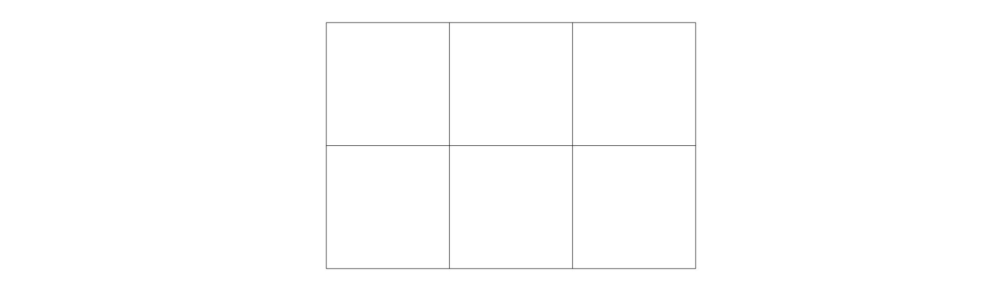
Fig. 1:

Let $j=k=1=j_{0}-1$. To see if (8) has a unique solution in $V_{h}^{0}$, we set $f=0$ and $v=u_{h}$. Then $\nabla_{w}u_{h}=0$. By definition,

$$0=(\nabla_{w}u_{h},\vec{q})_{{\cal T}_{h}}=-(u_{h},\nabla\vec{q})_{{\cal T}_{h}}+\left\langle u_{b},\vec{q}\cdot\vec{n}\right\rangle_{\partial{{\cal T}_{h}}},\quad\forall\vec{q}\in[P_{1}({\cal T}_{h})]^{2}.$$

Note that the degree of freedom of $[P_{1}({\cal T}_{h})]^{2}$ is $36$ while the degree of freedom of $V_{h}^{0}$ is $39$. Thus, there exist $u_{h}\neq 0$ so that $\nabla_{w}u_{h}=0$. Thus Algorithm $1$ will not work.

Example 2.2.

Let $\Omega=(0,1)\times(0,1)$ and is partitioned as shown in Figure 2.

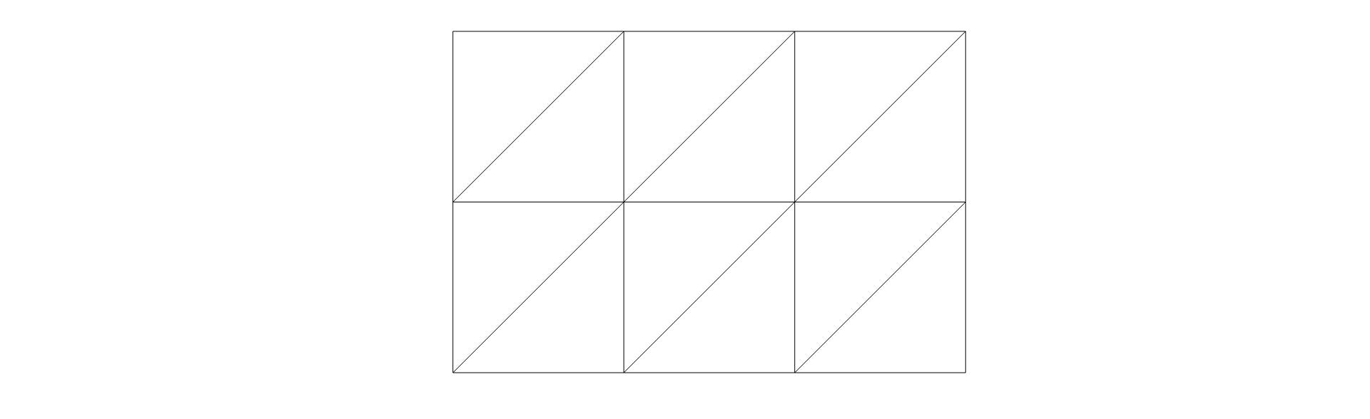
Fig. 2:

Let $j=k=1=j_{0}-1$. Note that the degree of freedom of $[P_{1}({\cal T}_{h})]^{2}$ is $72$ while the degree of freedom of $V_{h}^{0}$ is $75$. A similar argument as in example 2.1 shows that Algorithm $1$ will not work.

For the completeness, we list the following from [1].

Theorem 3.

Let $u_{h}\in V_{h}$ be the weak Galerkin finite element solution of (8). Assume that the exact solution $u\in H^{k+1}(\Omega)$ and $H^{2}$-regularity holds true. Then, there exists a constant $C$ such that

(34) $${|||}u-u_{h}{|||} \leq Ch^{k}|u|_{k+1},$$

(35) $$\|u-u_{0}\| \leq Ch^{k+1}|u|_{k+1}.$$

3 Numerical Experiments

We are devoting this section to verify our theoretical results in previous sections by two numerical examples. The domain in all examples is $\Omega=(0,1)\times(0,1)$. We will implement the SFWG finite element method (8) on triangular meshes. A uniform triangulation of the domain $\Omega$ is used. By refining each triangle for $N=2,4,8,16,32,64,128$, we obtain a sequence of partitions. The first two levels of grids are shown in Figure 3. We apply the SF-WG finite element method with $(P_{k}(T),P_{k}(e),[P_{k+1}(T)]^{2}),k=1,2$ finite element space to find SFWG solution $u_{h}=\{u_{0},u_{b}\}$ in the computation.

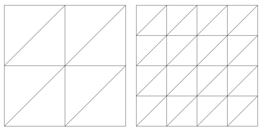
Fig. 3: The first two triangle grids in computation

Example 3.1.

In this example, we solve the Poisson problem (1)-(2) posed on the unit square $\Omega$, and the analytic solution is

(36) $$u(x,y)=\sin(\pi x)\sin(\pi y).$$

The boundary conditions and the source term $f(x,y)$ are computed accordingly. Table 1 lists errors and convergence rates in $H^{1}$-norm and $L^{2}$-norm.

Table 1: Error profiles and convergence rates for $P_{k}$ elements with $P_{k+1}^{2}$ weak gradient, $(k=1,2)$.

$k$	$h$	${|||}u_{h}-Q_{h}u{|||}$	Rate	$\|u_{0}-Q_{0}u\|$	Rate
	1/2	8.8205E-01	-	8.0081E-02	-
	1/4	4.3566E-01	1.02	2.5055E-02	1.68
	1/8	2.1565E-01	1.01	6.7091E-03	1.90
1	1/16	1.0747E-01	1.00	1.7092E-03	1.97
	1/32	5.3684E-02	1.00	4.2940E-04	1.99
	1/64	2.6836E-02	1.00	1.0749E-04	2.00
	1/128	1.3417E-02	1.00	2.6871E-05	2.00
	1/2	2.5893E-01	-	1.0511E-02	-
	1/4	6.5338E-02	1.99	1.2889E-03	3.03
	1/8	1.6252E-02	2.00	1.5596E-04	3.05
2	1/16	4.0538E-03	2.09	1.9193E-05	3.02
	1/32	1.0129E-03	2.00	2.3837E-06	3.00
	1/64	2.5321E-04	2.00	2.9713E-07	3.00
	1/128	6.3304E-05	2.00	3.7094E-08	3.00

Example 3.2.

In this example, we consider the problem $-\Delta u=f$ with boundary condition and the exact solution is

(37) $$u(x,y)=x(1-x)y(1-y).$$

The results obtained in Table 2 show the errors of SFWG scheme and the convergence rates in the ${|||}\cdot{|||}$ norm and $\|\cdot\|$ norm. The simulations are conducted on triangular meshes and polynomials of order $k=1,2$. The SFWG scheme with $P_{k}$ element has optimal convergence rate of $O(h^{k})$ in $H^{1}$-norm and $O(h^{k+1})$ in $L^{2}$-norm.

Table 2: Error profiles and convergence rates for $P_{k}$ elements with $P_{k+1}^{2}$ weak gradient, $(k=1,2)$.

$k$	$N$	${|||}e_{h}{|||}$	Rate	$\|e_{0}\|$	Rate
	1/2	5.6636E-02	-	5.3064E-03	-
	1/4	2.9670E-02	0.93	1.6876E-03	1.65
	1/8	1.4948E-02	0.99	4.5066E-04	1.90
1	1/16	7.4848E-03	1.00	1.1461E-04	1.98
	1/32	3.7435E-03	1.00	2.8778E-05	1.99
	1/64	1.8719E-03	1.00	7.2024E-06	2.00
	1/128	9.3596E-04	1.00	1.8011E-06	2.00
	1/2	1.3353E-02	-	5.6066E-04	-
	1/4	3.4831E-03	1.94	6.8552E-05	3.03
	1/8	8.7712E-04	1.99	8.2466E-06	3.06
2	1/16	2.1961E-04	2.00	1.0094E-06	3.03
	1/32	5.4967E-05	2.00	1.2482E-07	3.02
	1/64	1.3747E-05	2.00	1.5518E-08	3.00
	1/128	3.4375E-06	2.00	1.9344E-09	3.00

Overall, the numerical experiment’s results shown in the formentioned examples match the theoretical study part in the previous sections.

References

• [1] X. Ye, S. Zhang, On stabilizer-free weak Galerkin finite element method on polytopal meshes, arXiv:1906.06634v2, 2019.