Heterogeneous Regression Models for Clusters of Spatial Dependent Data

Abstract

In economic development, there are often regions that share similar economic characteristics, and economic models on such regions tend to have similar covariate effects. In this paper, we propose a Bayesian clustered regression for spatially dependent data in order to detect clusters in the covariate effects. Our proposed method is based on the Dirichlet process which provides a probabilistic framework for simultaneous inference of the number of clusters and the clustering configurations. The usage of our method is illustrated both in simulation studies and an application to a housing cost dataset of Georgia.

keywords: Clustered Coefficients Regression, Dirichlet process, MCMC, Spatial Random Effects

1 Introduction

Spatial regression models have been widely applied in many different fields such as environmental science (Hu and Bradley, 2018), biological science (Zhang and Lawson, 2011), and econometrics (Brunsdon et al., 1996) to explore the relation between a response variable and a set of predictors over a region. One of the most important tasks for a spatial regression model is to capture the spatial dependent structure between a response variable and a set of covariates. Cressie (1992) proposed a spatial regression model with Gaussian process, where the spatial random effects are accounted for only by the intercepts. Brunsdon et al. (1996) proposed a geographically weighted regression (GWR) model which assumed the existence of a spatially-dependent parameter surface, and used weighted local linear regression to estimate such parameter surface. An application of GWR in analyzing the impact of socio-economic factors on treated prevalence for mental disorders in Barcelona is presented in Salinas-Pérez et al. (2015). The idea of GWR has been subsequently extended to the Cox model framework by Xue et al. (2019). In addition to mean-based regression, Chasco and Gallo (2015) used a spatial quantile regression technique to identify heterogeneities. From the Bayesian perspective, Gelfand et al. (2003) incorporated Gaussian process to regression coefficients to build a model with spatially varying coefficients. Autant-Bernard and LeSage (2019) used a Bayesian heterogeneous spatial autoregressive model that allows for spatial variation variations in intercepts, covariate effects, and noise variances to study the knowledge production functions of different regions in order to set up their regional innovation strategy. The aforementioned works, however, all assumed that each location has its own set of regression parameters, which sometimes leads to excessive numbers of parameters, and subsequently overfitting. Cluster effects over the space of interest has not been taken into account.

Detection of heterogeneous covariate effects in many different fields, such as real estate applications, spatial econometrics, and environmental science are becoming of increasing research interest. For example, administrative divisions in a country, such as regions, provinces, states, or territories, often have different economic statuses and development patterns. More advanced divisions and less developed divisions could be put into separate clusters and analyzed. Such clustering information is of great interest to regional economics researchers. One of the most popular methods for spatial cluster detection is the scan statistic method (Kulldorff and Nagarwalla, 1995), where a scan statistic is constructed via a likelihood ratio statistic to test the potential clusters. The usage of spatial scan statistics has been extended to studies of disease mapping, crime, and public health. Similar endeavor has also been made under the Bayesian and nonparametric Bayesian frameworks in pursuit of spatial homogeneity. Li et al. (2015) used nonparametric Bayesian method to detect cluster boundaries for areal data. Noticing that traditional methods may not work well with spatial missing data, Panzera et al. (2016) proposed using multiple imputation together with the Bayesian Interpolation method to analyze spatially clustered missing data, which addresses both spatial univariate and multivariate problems.

Most of the aforementioned frequentist and Bayesian approaches mainly focus on estimating cluster configurations of spatial response. Spatially varying patterns in the relationship between a set of covariates and the response is also an important topic that needs to be studied. Billé et al. (2017) used a two-step approach where in the first step, spatial regimes of spatially varying parameters are identified, and in the second step estimated. Recently, methods for cluster detection of spatial regression coefficients have been proposed to detect the homogeneity of the covariates effects among subareas. Li and Sang (2019) incorporated spatial neighborhood information in a penalized approach to detect spatially clustered patterns in the regression coefficients.

Under the Bayesian framework, Lawson et al. (2014) explored the usage of multinomial priors in modeling clustered coefficients in the accelerated failure time model for survival data. As discussed by Lawson et al. (2014), to infer the grouping level, complicated search algorithms in variable dimensional parameter space are needed, such as the reversible jump Markov chain Monte Carlo (MCMC) algorithm of Green (1995), which assigns a prior on the number of clusters, and this number is updated at each iteration of an MCMC chain. Such algorithms are difficult to implement and automate, and are known to suffer from lack of scalability and mixing issues. Nonparametric Bayesian approaches, such as the Dirichlet process mixture model (DPMM; Ferguson, 1973), offer choices to allow for uncertainty in the number of clusters, and provide an integrated probabilistic framework under which the number of clusters, the clustering configuration, and regression coefficients are simultaneously estimated.

In this paper, we propose a Bayesian spatial clustered linear regression model with Dirichlet process (DP; Ferguson, 1973) prior, which considers spatially dependent structure and clusters the covariate effects simultaneously. In addition, implementation of our proposed methods based on nimble (de Valpine et al., 2017), a relatively new and powerful R package, is discussed. The model diagnostic technique, logarithm of the pseudo-marginal likelihood (LPML; Ibrahim et al., 2013), is introduced to assess the fitness of our proposed model. Our proposed Bayesian approach reveals interesting features of the state-level data of Georgia.

The remainder of the paper is organized as follows. In Section 2, we develop a spatial clustered linear regression model with DP prior. In Section 3, a MCMC sampling algorithm based on nimble and post MCMC inference are discussed. Extensive simulation studies are carried out in the next section. For illustration, our proposed methodology is applied to Georgia housing cost dataset in Section 5. Finally, we conclude this paper with a brief discussion.

2 Methodology

In this section, a Bayesian spatial clustered linear model using DPMM is proposed for coefficient grouping in spatially dependent data. Based on the spatial regression model, spatially-varying coefficients are assigned with a nonparametric DP prior to achieve the goal of grouping.

2.1 Spatial Regression Model

The basic geostatistical model (Gelfand and Schliep, 2016) for spatially dependent response at locations $\bm{s}=(s_{1},\ldots,s_{n})$ is denoted by

$$\bm{Y}=\bm{X}\bm{\beta}+\bm{w}+\bm{\epsilon},$$ (1)

where $\bm{Y}=(Y(s_{1}),\ldots,Y(s_{n}))$ the $n$-dimensional vector of responses observed at the $n$ different locations, $\bm{X}=\begin{pmatrix}X(s_{1})^{\top}\\ \ldots\\ X(s_{n})^{\top}\end{pmatrix}$ is the $n\times p$ matrix of covariates, $\bm{w}=(w(s_{1}),\ldots,w(s_{n}))$ is the vector of spatial random effects, which is assumed to follow a stationary Gaussian process whose covariance structure often depends on the geographical locations, and $\bm{\epsilon}\sim\mbox{MVN}(\bm{0},\sigma^{2}_{y}\bm{I})$ adds the nugget effect (see e.g., Chapter 6 of Carlin et al., 2014), which is usually a vector of white noise, with MVN denoting the multivariate normal distribution. Oftentimes, $\bm{w}(\bm{s})$ is assumed to also follow a MVN. The above spatial regression model can also be rewritten as

$$\begin{split}\bm{Y}\mid\bm{\beta},\bm{w},\sigma_{y}^{2}&\sim\mbox{MVN}(\bm{X}\bm{\beta}+\bm{w},\sigma_{y}^{2}\bm{I}),\\ \bm{w}&\sim\mbox{MVN}(\bm{0},\bm{\Sigma}_{W}),\end{split}$$

where  $\bm{\Sigma}_{W}$ is the covariance matrix of the spatial random effect vector $\bm{w}(\bm{s})$, and $\bm{I}$ denotes the identity matrix. Conditional on $\bm{X}$ and $\bm{w}$, entries in $\bm{Y}$ are independent. Conventionally, the covariance matrix is given as $\bm{\Sigma}_{W}=\sigma_{w}^{2}\bm{H}$, where $\bm{H}$ is a matrix constructed using the great circle distance matrix, denoted as GCD, between different locations, i.e.,

$$\mbox{GCD}=\mbox{GCD}(i,j)_{i,j\in\{1,\ldots,n\}}=\mbox{great circle distance between locations $s_{i}$ and $s_{j}$},$$

and $\sigma_{w}^{2}$ is a scalar. There are three common weighting schemes for defining $\bm{H}$, including:

$$\begin{split}\text{the unity scheme}:&~{}~{}\bm{H}=\bm{I}_{n\times n}\\ \text{the exponential scheme}:&~{}~{}\bm{H}(\phi)=\bm{H}(i,j)_{i,j\in\{1,\ldots,n\}}=\left[\exp(-\mbox{GCD}(i,j)/\phi)\right]_{n\times n},\\ \text{the Gaussian scheme}:&~{}~{}\bm{H}(\phi)=\bm{H}(i,j)_{i,j\in\{1,\ldots,n\}}=\left[\exp(-(\mbox{GCD}(i,j)/\phi)^{2})\right]_{n\times n},\end{split}$$ (2)

where $\phi$ is a tuning parameter that controls the spatial correlation. Larger value of $\phi$ indicates stronger correlation.

Another spatial regression model is the spatially varying coefficients model (Gelfand et al., 2003):

$$Y(s)=\bm{X}(s)^{\top}\widetilde{\bm{\beta}}(s)+\epsilon(s),$$ (3)

where $X(s)$ is $p\times 1$ covariate vector at a certain location $s$, and $\widetilde{\bm{\beta}}(s)$ is assumed to follow a $p$-variate spatial process model. If we have observations $(Y(s_{i}),\bm{X}(s_{i}))$ for $i=1,\ldots,n$, they can be written into

$$\bm{Y}=\bm{X}^{\top}\widetilde{\bm{\beta}}+\bm{\epsilon},$$

where $\bm{Y}=(Y(s_{1}),\ldots,Y(s_{n}))^{\top}$, $\bm{X}^{\top}$ is an $n\times(np)$ block diagonal matrix which has the row vector $\bm{X}^{\top}(s_{i})$ as its $i$-th diagonal entry, $\widetilde{\bm{\beta}}=(\widetilde{\bm{\beta}}(s_{1})^{\top},\ldots,\widetilde{\bm{\beta}}(s_{n})^{\top})^{\top}$, and $\bm{\epsilon}\sim\mbox{MVN}(\bm{0},\sigma^{2}\bm{I})$. Gelfand et al. (2003) proposed the following hierarchical model:

$$\begin{split}&\bm{Y}\mid\widetilde{\bm{\beta}},\sigma^{2}\sim\mbox{MVN}(\bm{X}^{\top}\widetilde{\bm{\beta}},\sigma^{2}\bm{I})\\ &{\widetilde{\bm{\beta}}}\mid\bm{\mu}_{\bm{\beta}},\bm{T}\sim\mbox{MVN}(1_{n\times 1}\otimes\bm{\mu}_{\bm{\beta}},\bm{H}(\phi)\otimes\bm{T})\end{split}$$ (4)

where $\bm{\mu}_{\bm{\beta}}$ is a $p\times 1$ vector, $\bm{H}(\phi)$ is a $n\times n$ matrix measuring spatial correlations between the $n$ observed locations, $\bm{T}$ is a $p\times p$ covariance matrix associated with an observation vector at any spatial location, and $\otimes$ denotes the Kronecker product. In model (1), $\bm{\beta}$ is constant over space, which means the covariate effects remain the same over all locations; model (4) allows for different covariate effects over locations, but restrict the covariate effects to be determined by distances between pairs of locations as in (2).

For many spatial economics data, however, some regions will share similar covariate effects regardless of their geographical distance. Taking China as an example, Beijing tends to have similar economic development pattern with Shanghai or Jiangsu (Ma et al., 2019b) . The models in (1) and (4), however, do not take into account such inherent similarities in spatially dependent data.

2.2 Spatial Regression with Dirichlet Process Mixture Prior

Within the Bayesian framework, coefficient clustering can be accomplished using a Dirichlet process mixture model (DPMM) by nonparametrically linking the spatial response variable to covariates through cluster membership. Formally, a probability measure $G$ following a DP with a concentration parameter $\alpha$ and a base distribution $G_{0}$ is denoted by $G\sim\text{DP}(\alpha,G_{0})$ if

$$(G(A_{1}),\cdots,G(A_{r}))\sim\text{Dirichlet}(\alpha G_{0}(A_{1}),\cdots,\alpha G_{0}(A_{r})),$$ (5)

where $(A_{1},\cdots,A_{r})$ are finite measurable partitions of the space $\Omega$. Several different formulations can be used for determining the DP. In this work, we use the stick-breaking construction proposed by Sethuraman (1991) for DP realization, which is given as

$$\theta_{c}\sim G_{0},~{}~{}G=\sum_{c=1}^{\infty}\pi_{c}\delta_{\theta_{c}}(\cdot),$$

$$\pi_{1}=V_{1},~{}~{}\pi_{c}=V_{c}\prod_{\ell<c}(1-V_{\ell}),$$

$$V_{c}\overset{\mbox{ind}}{\sim}\text{Beta}(1,\alpha),$$

where $\theta_{c}$ is the $c$-th vector consisting of the possible values of the parameters of $G_{0}$, $\delta_{\theta_{c}}(\cdot)$ denotes a discrete probability measure concentrated at $\theta_{c}$ and is a notation short for $\delta(\theta=\theta_{c})$, $\pi_{c}$ is the random probability weight between 0 and 1, and $\overset{\mbox{ind}}{\sim}$ indicates i.i.d..

For a DPMM, the observed data $y_{i}$ (for $i=1,\ldots,n$) follow an infinite mixture distribution, where a vector of latent allocation variables $\mathcal{Z}$ is introduced to enable explicit characterization of the clustering. Let $\mathcal{Z}_{n,k}=\big{\{}(z_{1},\ldots,z_{n}):z_{i}\in\{1,\ldots,k\},1\leq i\leq n\big{\}}$ denote all possible clusterings of $n$ observations into $k$ clusters, where $z_{i}=c\in\{1,\ldots,k\}$ denotes the cluster assignment of the $i$th observation. Note that although theoretically $c$ can go to infinity, in practice, with $n$ observations in total, $k$ is capped at $n$, which can only happen when each observation is assigned to its own cluster. The DPMM can be written as

$$\begin{split}y_{i}\mid\mathcal{Z},\theta&\sim f(y_{i}\mid\theta_{z_{i}}),\\ \theta_{c}&\sim G_{0},\\ P(z_{i}=c\mid&\bm{\pi})=\pi_{c},\\ \pi_{1}=V_{1},~{}~{}\pi_{c}=V_{c}\prod_{\ell<c}(&1-V_{\ell}),\hskip 2.84544ptV_{c}\overset{\mbox{ind}}{\sim}\text{Beta}(1,\alpha),\end{split}$$ (6)

where $\bm{\pi}=(\pi_{1},\ldots,\pi_{c},\ldots)$. Adapting the DPMM to the spatial regression setting, we focus on the clustering of spatially-varying coefficients $\bm{\beta}(s)=(\bm{\beta}^{\top}(s_{1}),\cdots,\bm{\beta}^{\top}(s_{n}))^{\top}$, where $\bm{\beta}(s_{i})$ is the $p$-dimensional coefficient vector for location $s_{i}$. In our setting, we assume that the $n$ parameter vectors can be clustered into $k$ groups, i.e., $\bm{\beta}(s_{i})=\bm{\beta}_{z_{i}}\in\{\bm{\beta}_{1},\ldots,\bm{\beta}_{k}\}$, then the model can be written as

$$y(s_{i})\mid\bm{\beta}_{z_{i}}{{\color[rgb]{0,0,0},}}w(s_{i}),\sigma_{y}^{2} \sim N(\bm{X}(s_{i})^{\top}\bm{\beta}(s_{z_{i}})+w(s_{i}),\sigma_{y}^{2}),$$ (7)

$$\bm{w}(\bm{s}) \sim\mbox{MVN}(\bm{0},\bm{\Sigma}_{W}),$$ (8)

$$\bm{\beta}_{z_{i}} \stackrel{{\scriptstyle\text{ind}}}{{\sim}}\mbox{MVN}(\bm{\mu},\bm{\Sigma}),$$ (9)

$$P( z_{i}=c\mid\bm{\pi})=\pi_{c},$$ (10)

$$\pi_{1}=V_{1},~{}~{}\pi_{c}=V_{c} \prod_{\ell<c}(1-V_{\ell}),~{}~{}V_{c}\overset{\mbox{ind}}{\sim}\text{Beta}(1,\alpha).$$ (11)

3 Bayesian Inference

MCMC is used to draw samples from the posterior distributions of the model parameters. In this section we present the sampling scheme, the posterior inference of cluster belongings, and measurements to evaluate the estimation performance and clustering accuracy.

3.1 The MCMC Sampling Scheme

We present the main R function written using the nimble package (de Valpine et al., 2017). The model is wrapped in a nimbleCode() function. For ease of exposition, we break it into separate snippets. The full code is available on GitHub with an example implementation. (link removed for blinding purposes, documentation submitted separately)

Define S as the number of locations. The following code represent Equation (7). At each location, y[i] has a normal distribution with mu_y[i] and precision tau_y, which is equivalent to $1/\sigma_{y}^{2}$. A Gamma(1,1) prior is given to tau_y. The coefficient vector for location i, b[i, 1:6], equals the coefficient vector estimated for the cluster it belongs to, represented by latent[i], which follows a multinomial distribution with probability vector zlatent[1:M], where M denotes the number of potential clusters.

SLMMCode <- nimbleCode({
  for (i in 1:S) {
    y[i] ~ dnorm(mu_y[i], tau = tau_y)
    mu_y[i] <- b[i, 1] * x1[i] + b[i, 2] * x2[i] +
      b[i, 3] * x3[i] + b[i, 4] * x4[i] + b[i, 5] * x5[i] +
      b[i, 6] * x6[i] + W[i]

    b[i, 1:6] <- bm[latent[i], 1:6]

    latent[i] ~ dcat(zlatent[1:M])
  }

The following code represent Equation (8). H represents the matrix $\Sigma_{W}$, where phi is the tuning parameter $\phi$ in the exponential scheme in (2) that controls spatial correlation. The random effects at locations 1 to S follow a multivariate normal distribution with mu_w[1:S] and precision matrix, which equals the product of $\sigma_{w}^{2}$, tau_w, and the inverse of H. H is defined as a function of a certain distance matrix Dist, which is passed into the function later as an argument of SLMMConsts. Here, the function is chosen to be the exponential scheme. The prior distribution of the bandwidth phi is specified to be a uniform distribution from 0 to a certain upper limit, denoted by D. The prior of tau_w is set to Gamma(1,1).

  for (j in 1:S) {
    for (k in 1:S) {
      H[j, k] ¡- exp(-Dist[j, k]/phi)
    }
  }

  W[1:S] ~ dmnorm(mu_w[1:S], prec = prec_W[1:S, 1:S])
  prec_W[1:S, 1:S] ¡- tau_w * inverse(H[1:S, 1:S])

  phi ~ dunif(0, D)
  tau_w ~ dgamma(1, 1)

  mu_w[1:S] ¡- rep(0, S)

The distribution of $\bm{\beta}$ for each location $s_{i}$ is defined next. They each come from a multivariate normal distribution with mean mu_bm and covariance matrix var_bm, which is a diagonal matrix with all diagonal entries being 1/tau_bm. The inverse variance term, tau_bm, is again given a Gamma(1,1) prior, and the entries in the mean vector are all given independent standard normal priors.

  for (k in 1:M) {
    bm[k, 1:6] ~ dmnorm(mu_bm[1:6], cov = var_bm[1:6, 1:6])
  }
  var_bm[1:6, 1:6] ¡- 1/tau_bm * diag(rep(1, 6))
  tau_bm ~ dgamma(1, 1)

  for (j in 1:6) {
    mu_bm[j] ~ dnorm(0, 1)
  }

Finally for the model, the stick breaking process corresponding to Equations (10) and (11) is depicted.

  zlatent[1:M] <- stick_breaking(vlatent[1:(M - 1)])

  for (j in 1:(M - 1)) {
    vlatent[j] ~ dbeta(1, alpha)
  }

  alpha ~ dgamma(1, 1)
  tau_y ~ dgamma(1, 1)

})

With the full model defined, we next declare the data list, which is made up of the response Y, the covariates X[,1] to X[,6], and the matrix of distances Dist. The constants in the model also need to be supplied, including the number of locations S, the number of starting clusters M, and the upper endpoint D for the uniform distribution of bandwidth. In addition, the initial values are specified. Code to compile the model, supply the initial values, and invoke the MCMC process is included in the supplementary package.

SLMMdata ¡- list(y = y, x1 = X[,1], x2 = X[,2], x3 = X[,3],
                 x4 = X[,4], x5 = X[,5], x6 = X[,6],
                 Dist = distmatrix)

SLMMConsts ¡- list(S = 159, M = 50, D = 100)

SLMMInits ¡- list(tau_y = 1,
                  latent = rep(1, SLMMConsts$S), alpha = 2,
                  tau_bm = 1,
                  mu_bm = rnorm(6), phi = 1, tau_w = 1,
                  vlatent = rbeta(SLMMConsts$M - 1, 1, 1)
)

3.2 Inference of MCMC results

The estimated parameters, together with the cluster assignments $\bm{z}$, are determined for each replicate from the best post burn-in iteration selected using the Dahl’s method (Dahl, 2006). Dahl (2006) proposed a least-square model-based clustering for estimating the clustering of observations using draws from a posterior clustering distribution. In this method, membership matrices for each iteration, $\bm{B}^{(1)},\ldots,\bm{B}^{(M)}$, where $M$ is the number of post-burn-in MCMC itertations, are calculated. The membership matrix for the $c$th iteration, $\bm{B}^{(c)}$ is defined as:

$$\bm{B}^{(c)}=(\bm{B}^{(c)}(i,j))_{i,j\in\{1:n\}}=1(z_{i}^{(c)}=z_{j}^{(c)})_{n\times n},$$ (12)

with $1()$ being the indicator function, $\bm{B}^{(c)}(i,j)\in\{0,1\}$ for all $i,j=1,...,n$ and $c=1,\ldots,M$. Having $\bm{B}^{(c)}(i,j)=1$ means observations $i$ and $j$ are in the same cluster in the $c$th iteration. The average of $\bm{B}^{(1)},\ldots,\bm{B}^{(M)}$ can be calculated as

$$\overline{\bm{B}}=\frac{1}{M}\sum_{c=1}^{M}\bm{B}^{(c)},$$

where $\sum$ here denotes element-wise summation of matrices. The $(i,j)$th entry of $\overline{\bm{B}}$ provides an empirical estimate of the probability for locations $i$ and $j$ to be in the same cluster.

Next we find the iteration that has the least squared distance to $\overline{\bm{B}}$ as:

$$C_{LS}=\operatorname*{arg\,min}_{c\in(1:M)}\sum_{i=1}^{n}\sum_{j=1}^{n}\left(\bm{B}^{(c)}(i,j)-\overline{\bm{B}}(i,j)\right)^{2},$$ (13)

where $\bm{B}^{(c)}(i,j)$ is the ($i,j$)th entry of $\bm{B}^{(c)}$, and $\overline{\bm{B}}(i,j)$ is the ($i,j$)th entry of $\overline{\bm{B}}$. An advantage of the least-squares clustering is the fact that information from all clusterings are utilized via the usage of the empirical pairwise probability matrix $\overline{\bm{B}}$. It is also intuitively appealing, as the average clustering is selected instead of formed via an external, ad hoc clustering algorithm.

3.3 Model Assessment

In the spatial regression model, the Gaussian process spatial structure $\bm{\Sigma_{W}}=\sigma_{w}^{2}\bm{H}$ can be constructed via several different weighting schemes including the aforementioned unity, exponential, and Gaussian schemes in (2). In order to determine which weighting scheme is the most suitable for the data, a commonly used model comparison criterion, the logarithm of the pseudo-Marginal likelihood (LPML; Ibrahim et al., 2013), is applied. The LPML can be obtained through the conditional predictive ordinate (CPO) values. With $Y^{*}_{(-i)}=(Y_{1},\ldots,Y_{i-1},Y_{i+1},\ldots,Y_{n})$ denoting the observations with the $i$th subject response deleted, CPO can be regarded as leave-one-out-cross-validation under Bayesian framework, and it estimates the probability of observing $Y_{i}$ in the future if after having already observed $Y^{*}_{(-i)}$. The CPO for the $i$th subject is calculated as:

$$\text{CPO}_{i}=\int f(y(s_{i})\mid\bm{\beta}(s_{i}),w(s_{i}),\sigma_{y}^{2})\pi(\bm{w}(\bm{s}),\bm{\beta}(\bm{s}),\sigma_{y}^{2}\mid Y^{*}_{(-i)})\differential(\bm{w}(\bm{s}),\bm{\beta}(\bm{s}),\sigma_{y}^{2}),$$ (14)

where

$$\pi(\bm{w}(\bm{s}),\bm{\beta}(\bm{s}),\sigma_{y}^{2}\mid Y^{*}_{(-i)})=\frac{\prod_{j\neq i}f(y(s_{j})\mid\bm{\beta}(s_{j}),w(s_{j}),\sigma_{y}^{2})\pi(\bm{w}(\bm{s}),\bm{\beta}(\bm{s}),\sigma_{y}^{2}\mid Y^{*}_{(-i)})}{c(Y^{*}_{(-i)})},$$

and $c(Y^{*}_{(-i)})$ is the normalizing constant. Within the Bayesian framework, a Monte Carlo estimate of the CPO can be obtained as:

$$\widehat{\text{CPO}}_{i}^{-1}=\frac{1}{M}\sum_{t=1}^{M}\frac{1}{f(y(s_{i})\mid w_{t}(s_{i}),\bm{\beta}_{t}(s_{i}),\sigma_{yt}^{2})},$$ (15)

where $w_{t}(s_{i})$ is calculated based on the sampled $\phi$ in the $t$-th iteration, and $\bm{\beta}_{t}(s_{i})$ and $\sigma_{yt}^{2}$ are, respectively, the $t$-th iteration samples for $\bm{\beta}(s_{i})$ and $\sigma_{y}^{2}$. An estimate of the LPML can subsequently be calculated as:

$$\widehat{\text{LPML}}=\sum_{i=1}^{N}\log(\widehat{\text{CPO}}_{i}).$$ (16)

A model with a larger LPML value is preferred. In addition, $p_{D}$, the effective number of parameters, which can be used to measure the complexity of the model, is defined as

$$p_{D}=\overline{D}-D(\overline{\bm{\theta}}),$$ (17)

where $D=-2\log f(\bm{y}(\bm{s})\mid\bm{\theta})$ is the deviance of the model, $\overline{D}$ is the posterior mean of deviance, $\overline{\bm{\theta}}$ is the posterior mean of the parameters and $D(\overline{\bm{\theta}})$ denotes deviance at posterior means.

3.4 Convergence Diagnostics

We use the Rand index (RI; Rand, 1971) to measure the accuracy of clustering. The RI is defined as

$$\mathrm{RI}=(a+b)/(a+b+c+d)=(a+b)\left.\right/{n\choose 2},$$

where $\mathcal{C}_{1}=\{X_{1},\ldots,X_{r}\}$ and $\mathcal{C}_{2}=\{Y_{1},\ldots,Y_{s}\}$ are two partitions of $\{1,2,\ldots,n\}$, and $a,b,c$ and $d$ respectively denote the number of pairs of elements of $\{1,2,\ldots,n\}$ that are (a) in a same set in $\mathcal{C}_{1}$ and a same set in $\mathcal{C}_{2}$, (b) in different sets in $\mathcal{C}_{1}$ and different sets in $\mathcal{C}_{2}$, (c) in a same set in $\mathcal{C}_{1}$ but in different sets in $\mathcal{C}_{2}$, and (d) in different sets in $\mathcal{C}_{1}$ and a same set in $\mathcal{C}_{2}$. The RI ranges from 0 to 1 with a higher value indicating better agreement between the two partitions. In particular, $\mathrm{RI}=1$ indicates that $\mathcal{C}_{1}$ and $\mathcal{C}_{2}$ are identical in terms of modulo labeling of the nodes.

4 Simulation Studies

In this section, we conduct simulation studies to assess the performance of the proposed methods under scenarios where there is no clustered covariate effect, and when there is indeed clustered covariate effect. All simulations are run on an institutional high performance computing cluster running Red Hat Enterprise Linux Server (release 6.7).

4.1 Simulation Without Clustered Covariate Effects

The spatial adjacency structure of counties in Georgia is used. As a starting point, to mimic the real dataset we use later, one observation is generated for each of the 159 counties. Six covariate vectors are generated for the 159 counties with each entry i.i.d. from $N(0,1)$, making a $159\times 6$ covariate matrix $\bm{X}$. The spatial random effects $\bm{w}$ are simulated based on the matrix of great circle distance (GCD) between county centroids. The great circle distances are obtained using the function distCosine(), and the centroids are calculated based on county polygons using the function centroid(), both provided by the R package geosphere (Hijmans, 2017). The GCD matrix is subsequently normalized to have a maximum value of 10 for ease in computation. and the response vector $\bm{Y}$ is generated as

$$\bm{Y}=\bm{X}\bm{\beta}+\bm{w}+\bm{\epsilon},$$

where $\bm{X}=(X_{1},\ldots,X_{6})$, $\bm{w}\sim\text{MVN}(\bm{0},\exp(-\mbox{GCD}/4))$, and $\bm{\epsilon}\sim\mbox{MVN}(\bm{0},\bm{I})$. Different values of $\bm{\beta}$ are used: $(1,0,1,0,0.5,2)^{\top}$, $(2,0,1,0,4,2)^{\top}$, and $(9,0,-4,0,2,5)^{\top}$, corresponding to scenarios where the signal is weak, moderate, and strong. For each of the three $\bm{\beta}$’s, the average parameter estimate denoted by $\overline{\widehat{\beta}}_{\ell,m}$ ($\ell=1,\cdots,159$; $m=1,\cdots,6$) in 100 simulations is calculated as

$$\overline{\widehat{\beta}}_{\ell,m}=\frac{1}{100}\sum_{r=1}^{100}\widehat{\beta}_{\ell,m,r},$$ (18)

where $\widehat{\beta}_{\ell,m,r}$ denotes the posterior estimate for the $m$th coefficient of county $\ell$ in the $r$th replicate. The performance of these posterior estimates are evaluated by the mean absolute bias (MAB), the mean standard deviation (MSD), the mean of mean squared error (MMSE) and mean coverage rate (MCR) of the 95% highest posterior density (HPD) intervals in the following ways:

MAB $$=\frac{1}{159}\sum_{\ell=1}^{159}\frac{1}{100}\sum_{r=1}^{100}\left|\widehat{\beta}_{\ell,m,r}-\beta_{\ell,m}\right|,$$ (19)

MSD $$=\frac{1}{159}\sum_{\ell=1}^{159}\sqrt{\frac{1}{99}\sum_{r=1}^{100}\left(\widehat{\beta}_{\ell,m,r}-\overline{\widehat{\beta}}_{\ell,m}\right)^{2}},$$ (20)

MMSE $$=\frac{1}{159}\sum_{\ell=1}^{159}\frac{1}{100}\sum_{r=1}^{100}\left(\widehat{\beta}_{\ell,m,r}-\beta_{\ell,m}\right)^{2},$$ (21)

MCR $$=\frac{1}{159}\sum_{\ell=1}^{159}\frac{1}{100}\sum_{r=1}^{100}1\left(\widehat{\beta}_{\ell,m,r}\in\text{95\% HPD interval}\right),$$ (22)

In each replicate, the MCMC chain length is set to be 50,000, with thinning 10 and the first 2,000 samples are discarded as burn-in, therefore we have 3,000 samples for posterior inference. The parameter $D$ for the uniform prior of bandwidth, i.e. $\phi$ in Equation (2), is set to 100 such that the prior for bandwidth is also noninformative. In Table 1 the average parameter estimates $\overline{\widehat{\beta}}_{\ell,m}$ are reported together with the four performance measures in Equations (19),(20), (21) and (22) are reported for the three settings. Under all three settings, the parameter estimates are highly close to the true underlying values, and have very small MAB, MSD and MMSE, while maintaining the MCR at close to 95% level. The RI’s are all very close to or equal to 1, indicating that the clustering results are highly consistent and credible. It is worth noticing that, even when the signal is relatively weak, the clustering approach is quite precise.

Table 1: Average parameter estimates and performance of parameter estimates and clustering results when without clustered covariate effect.

		$\overline{\widehat{\beta}}$	MAB	MSD	MMSE	MCR	RI
Setting 1	$\beta_{1}$	1.005	0.110	0.085	0.007	0.910	0.997
	$\beta_{2}$	0.002	0.087	0.069	0.005	0.980
	$\beta_{3}$	0.996	0.104	0.076	0.006	0.950
	$\beta_{4}$	-0.003	0.090	0.071	0.005	0.970
	$\beta_{5}$	0.508	0.106	0.080	0.006	0.960
	$\beta_{6}$	1.978	0.109	0.081	0.007	0.970
Setting 2	$\beta_{1}$	1.971	0.218	0.117	0.014	0.930	0.999
	$\beta_{2}$	-0.001	0.090	0.072	0.005	0.980
	$\beta_{3}$	0.987	0.129	0.085	0.007	0.960
	$\beta_{4}$	0.002	0.098	0.076	0.006	0.950
	$\beta_{5}$	3.934	0.362	0.145	0.021	0.910
	$\beta_{6}$	1.955	0.194	0.105	0.011	0.960
Setting 3	$\beta_{1}$	9.006	0.108	0.081	0.007	0.930	1.000
	$\beta_{2}$	-0.001	0.088	0.069	0.005	0.970
	$\beta_{3}$	-3.996	0.089	0.069	0.005	0.960
	$\beta_{4}$	-0.002	0.091	0.072	0.005	0.960
	$\beta_{5}$	2.007	0.106	0.081	0.007	0.950
	$\beta_{6}$	4.990	0.090	0.071	0.005	0.960

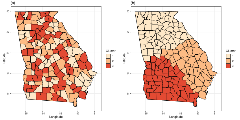
Figure 1: Visualization of (a) random cluster assignment and (b) regional cluster assignment for Georgia counties used for simulation studies.

4.2 Simulation with Clustered Covariate Effects

We consider an underlying setting where there exist clustered covariate effects. First we consider a setting where the clustered covariate effect is independent of spatial locations, i.e. where cluster belonging are set randomly. The 159 counties are randomly assigned to three clusters, visualized in Figure 1(a). There are, respectively, 51, 49, and 59 counties in the three clusters. Different parameter vectors are used for data generation in different clusters (see Table 2) to assess the estimation and clustering performance under different strengths of signals. The spatial random effect $\bm{W}$ is generated using the same setting as before. The performance measures are presented in Table 3. In another scenario, a setting where the clustered covariate effect depends on spatial locations. Consider a partition of Georgia counties into three large regions, visualized in Figure 1(b). The same parameter vectors in Table 2 are used for the three clusters under three settings. Corresponding performance measures are reported in Table 4.

For each signal strength and each of the two settings, we randomly selected four replicates from the total of 100 replicates and visualize the results in the Online Supplement. It is no surprise that under both settings, the accuracy of clustering increases with the strengthening of signals. It can be seen from Supplemental Figures 1 and 4 that with weak true signals, the proposed approach suffers from over-clustering, which is a known property of Dirichlet process mixtures that the posterior does not concentrate at the true number of clusters (see, e.g., Miller and Harrison, 2013). This over-clustering behavior, however, diminishes as the signals’ strength increase. When the signals are strong, the RI reaches near 0.85, indicating that 85% of the time, two counties that belong to the same cluster are correctly put into the same cluster. Together with increase in RI is decrease in MCR, which is an inevitable result of incorporating more counties in each cluster. For each county, taking other counties that do not belong to this county’s true cluster introduces bias in estimation.

Table 2: True parameter vectors used in data generation for three clusters.

	Cluster 1	Cluster 2	Cluster 3
Setting 1	(1, 0, 1, 0, 0.5, 2)	(1, 0.7, 0.3, 2, 0, 3)	(2, 1, 0.8, 1, 0, 1)
Setting 2	(2, 0, 1, 0, 4, 2)	(1, 0, 3, 2, 0, 3)	(4, 1, 0, 3, 0, 1)
Setting 3	(9, 0, -4, 0, 2, 5)	(1, 7, 3, 6, 0, -1)	(2, 0, 6, 1, 7, 0)

Table 3: Performance of parameter estimates and clustering results under the scenario where cluster belongings are set randomly.

		MAB	MSD	MMSE	MCR	RI
Setting 1	$\beta_{1}$	0.186	0.421	0.242	0.935	0.621
	$\beta_{2}$	0.173	0.401	0.180	0.967
	$\beta_{3}$	0.150	0.293	0.093	0.985
	$\beta_{4}$	0.206	0.721	0.672	0.924
	$\beta_{5}$	0.168	0.241	0.063	0.977
	$\beta_{6}$	0.227	0.747	0.705	0.916
Setting 2	$\beta_{1}$	0.967	0.812	0.735	0.757	0.690
	$\beta_{2}$	0.443	0.378	0.150	0.834
	$\beta_{3}$	0.958	0.806	0.743	0.753
	$\beta_{4}$	0.961	0.826	0.698	0.762
	$\beta_{5}$	1.390	1.071	1.339	0.786
	$\beta_{6}$	0.670	0.608	0.408	0.766
Setting 3	$\beta_{1}$	1.941	0.763	0.636	0.816	0.852
	$\beta_{2}$	1.870	0.728	0.602	0.867
	$\beta_{3}$	2.310	0.933	0.940	0.828
	$\beta_{4}$	1.491	0.636	0.445	0.814
	$\beta_{5}$	1.700	0.738	0.606	0.845
	$\beta_{6}$	1.442	0.600	0.388	0.828

Table 4: Performance of parameter estimates and clustering results under the scenario where cluster belongings are set depending on the county centroid locations.

		MAB	MSD	MMSE	MCR	RI
Setting 1	$\beta_{1}$	0.201	0.413	0.237	0.966	0.597
	$\beta_{2}$	0.154	0.426	0.195	0.977
	$\beta_{3}$	0.165	0.289	0.091	0.991
	$\beta_{4}$	0.216	0.720	0.657	0.937
	$\beta_{5}$	0.182	0.256	0.068	0.988
	$\beta_{6}$	0.210	0.683	0.619	0.904
Setting 2	$\beta_{1}$	0.885	0.806	0.782	0.787	0.691
	$\beta_{2}$	0.425	0.353	0.138	0.860
	$\beta_{3}$	0.789	0.783	0.832	0.802
	$\beta_{4}$	0.969	0.856	0.758	0.783
	$\beta_{5}$	1.437	1.106	1.280	0.789
	$\beta_{6}$	0.585	0.592	0.432	0.807
Setting 3	$\beta_{1}$	1.981	0.764	0.625	0.831	0.855
	$\beta_{2}$	1.711	0.706	0.710	0.855
	$\beta_{3}$	2.389	0.951	0.983	0.838
	$\beta_{4}$	1.363	0.609	0.486	0.852
	$\beta_{5}$	1.617	0.724	0.634	0.830
	$\beta_{6}$	1.471	0.603	0.389	0.838

5 Real Data Analysis

We consider analyzing influential factors for monthly housing cost in Georgia using the proposed methods. The dataset is available at www.healthanalytics.gatech.edu, with 159 observations corresponding to the 159 counties in Georgia. For each county, the dependent variable median monthly housing cost for all occupied housing units is observed. The independent variables considered here include: the percentage of adults aged 18 to 64 who are unemployed ($X_{1}$), the average total real and personal property taxes collected per person ($X_{2}$), the median home market value ($X_{3}$, in thousand dollars), the percentage of White race population ($X_{4}$), the median age ($X_{5}$), and size of a county’s population ($X_{6}$, in thousands). Figure 2 provides a visualization of the 6 covariates on the Georgia map. In the computation, the covariates are centered and scaled to have mean 0 and unit standard deviation. Also, following the common practice in economics to account for long-tailed distributions, we take the logarithm of monthly housing cost before fitting the model. The response variable is also centered and scaled, and therefore all models to follow are fitted without the intercept term.

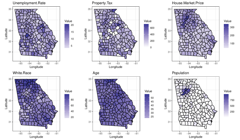
Figure 2: Visualizations of covariate values in counties of Georgia.

We firstly apply the model assessment criteria, LPML, for selecting the best weighting scheme for the data. The LPML values for the unity weighting scheme, the exponential weighting scheme and the Gaussian weighting scheme are shown in Table 5. From Table 5 we can see that the model with exponential weighting scheme has the largest LPML value among the three candidate schemes, and is therefore preferred. To verify that there is indeed spatially varying covariate effects, we also fitted the spatially-varying coefficients model without clustering (4) to the dataset. The model is also compared against a vanilla Bayesian regression, where no spatial effect is considered, and observations are treated as i.i.d. samples from the population. In this model, no spatial variation is assumed in the covariate effects $\bm{\beta}$, and the model reduces to the regular Bayesian linear regression.

The computation is performed on a desktop computer running Windows 10 Enterprise, with i7-8700K CPU @ 3.70GHz. The computing time as well as performance measure for these three models are recorded and presented in Table 6. The proposed model takes around 650 seconds to run, followed by the spatially varying coefficients model, and then the spatially constant coefficients model. The LPML values of the first two models that allow for spatially varying coefficients are larger than the vanilla regression model, and the differences are not minor. This indicates that there indeed exist spatially varying covariate effect, and more flexible models are preferred. Comparing the LPML and $p_{D}$ for the first two models, it can be seen that the proposed model reduces $p_{D}$ and provides better fit to the data. Combining the conclusions from Tables 5 and 6, the proposed model with exponential weighting scheme for $\bm{W}(s)$ is fitted on the dataset.

Table 5: LPML values for different weighting schemes in the proposed model.

	Unity	Exponential	Gaussian
LPML	-165.784	-165.620	-217.878

Table 6: LPML and $p_{D}$ values and computing time for different models.

	The proposed model	Spatial-varying coefficients model	Vanilla regression
LPML	-165.620	-174.171	-203.013
$p_{D}$	75.17	105.92	11.44
Time (seconds)	653.00	318.24	260.55

A total of 3 clusters are identified. The cluster belongings of the 159 counties are visualized in Figure 3, and their corresponding parameter estimates are presented in Table 7. From Figure 3 we can find that the cluster distribution is more similar with the spatial distributions of the covariates population size and median home market price. These two covariates also show great impact on cluster 1, the largest cluster we obtained from the model. For cluster 1, which includes most of the counties (124 out of 159), higher unemployment rates, higher median home market value, and larger population sizes are significant indicators of higher housing costs. For cluster 2 (26 out of 159), median home market value is also positively correlated with the monthly housing cost, while higher median age indicates lower housing cost. For cluster 3 (9 out of 159) median home market value turns out to be the only decisive factor and has significant increasing effect for housing cost. These results indicate that for most counties of Georgia, unemployment rates, median home market value and population size drive the variation of housing costs greatly. However, not all the counties have the same pattern. Housing costs of some counties are affected by median home market price and median age instead, and for a few counties, the housing costs are related to median home market value instead of the other covariates. This example here verifies the fact that the proposed model can detect the spatial clusters which share similar covariate effects.

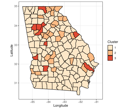
Figure 3: Clusters produced by the proposed approach.

Table 7: Parameter estimates and their 95% HPD intervals for the three clusters identified.

Cluster	1	2	3
$\widehat{\beta}_{1}$	0.154	-0.088	-0.349
	(0.020, 0.293)	(-0.424, 0.394)	(-1.533, 0.811)
$\widehat{\beta}_{2}$	-0.091	0.043	-0.047
	(-0.217, 0.040)	(-0.404, 0.433)	(-1.19, 1.08)
$\widehat{\beta}_{3}$	1.841	1.985	1.540
	(1.615, 2.072)	(1.463, 2.580)	(0.317, 2.778)
$\widehat{\beta}_{4}$	-0.078	-0.146	0.151
	(-0.295, 0.102)	(-0.648, 0.313)	(-0.910, 1.509)
$\widehat{\beta}_{5}$	-0.004	-0.998	-0.994
	(-0.205, 0.192)	(-1.478, -0.578)	(-1.899, 0.186)
$\widehat{\beta}_{6}$	0.327	0.611	0.119
	(0.069, 0.698)	(-0.592, 1.421)	(-0.789, 1.435)

6 Discussion

In this paper, we have proposed a Bayesian clustered coefficients linear regression model with spatial random effects to capture heterogeneity of regression coefficients. Multiple weighting schemes in modeling the spatial random effects have been proposed, and the corresponding Bayesian model selection criterion have been discussed. Compared to a vanilla regression model with no spatial random effect, allowing the covariate effects to be spatially varying provides better fit to the data, and more profound insight into heterogeneity in development at different locations. In addition, compared to observations made in Ma et al. (2019a), where each location is allowed to have its own set of parameter estimates, the clustering approach reduces the effective number of parameters without sacrificing the model goodness-of-fit. The usage of the method is illustrated both in simulation studies and an application to analysis of impacting factors for housing cost in Georgia.

A few topics beyond the scope of this paper are worth further investigation. In this paper, we only considered the full model that includes all covariates. Appropriate approaches for variable selection under a clustered regression context is worth investigating. The DPMM is used to get clustering information of regression coefficients. The posterior on the number of clusters is not consistent based on the DPMM. Such pattern have been observed in both our simulation studies, where there are some small clusters which only contain a few counties. Proposing a consistent prior (Geng et al., 2019; Hu et al., 2020) for clustered regression coefficients is an important future work. In addition, extending our approach in non-gaussian model is an interesting topic. Considering spatial dependent structure for the regression coefficients (Zhao et al., 2020) is devoted to future research.

References

- Autant-Bernard and LeSage (2019) Autant-Bernard, C. and J. P. LeSage (2019). A heterogeneous coefficient approach to the knowledge production function. Spatial Economic Analysis 14(2), 196–218.
- Billé et al. (2017) Billé, A. G., R. Benedetti, and P. Postiglione (2017). A two-step approach to account for unobserved spatial heterogeneity. Spatial Economic Analysis 12(4), 452–471.
- Brunsdon et al. (1996) Brunsdon, C., A. S. Fotheringham, and M. E. Charlton (1996). Geographically weighted regression: a method for exploring spatial nonstationarity. Geographical Analysis 28(4), 281–298.
- Carlin et al. (2014) Carlin, B. P., A. E. Gelfand, and S. Banerjee (2014). Hierarchical Modeling and Analysis for Spatial Data. Chapman and Hall/CRC.
- Chasco and Gallo (2015) Chasco, C. and J. L. Gallo (2015). Heterogeneity in perceptions of noise and air pollution: A spatial quantile approach on the city of Madrid. Spatial Economic Analysis 10(3), 317–343.
- Cressie (1992) Cressie, N. (1992). Statistics for spatial data. Terra Nova 4(5), 613–617.
- Dahl (2006) Dahl, D. B. (2006). Model-based clustering for expression data via a Dirichlet process mixture model. Bayesian Inference for Gene Expression and Proteomics 4, 201–218.
- de Valpine et al. (2017) de Valpine, P., D. Turek, C. J. Paciorek, C. Anderson-Bergman, D. T. Lang, and R. Bodik (2017). Programming with models: writing statistical algorithms for general model structures with NIMBLE. Journal of Computational and Graphical Statistics 26(2), 403–413.
- Ferguson (1973) Ferguson, T. S. (1973). A Bayesian analysis of some nonparametric problems. Annals of Statistics 1(2), 209–230.
- Gelfand et al. (2003) Gelfand, A. E., H.-J. Kim, C. Sirmans, and S. Banerjee (2003). Spatial modeling with spatially varying coefficient processes. Journal of the American Statistical Association 98(462), 387–396.
- Gelfand and Schliep (2016) Gelfand, A. E. and E. M. Schliep (2016). Spatial statistics and Gaussian processes: A beautiful marriage. Spatial Statistics 18, 86–104.
- Geng et al. (2019) Geng, J., A. Bhattacharya, and D. Pati (2019). Probabilistic community detection with unknown number of communities. Journal of the American Statistical Association 114(526), 893–905.
- Green (1995) Green, P. J. (1995). Reversible jump Markov chain Monte Carlo computation and Bayesian model determination. Biometrika 82(4), 711–732.
- Hijmans (2017) Hijmans, R. J. (2017). geosphere: Spherical Trigonometry. R package version 1.5-7.
- Hu and Bradley (2018) Hu, G. and J. Bradley (2018). A Bayesian spatial-temporal model with latent multivariate log-gamma random effects with application to earthquake magnitudes. Stat 7(1), e179. e179 sta4.179.
- Hu et al. (2020) Hu, G., J. Geng, Y. Xue, and H. Sang (2020). Bayesian spatial homogeneity pursuit of functional data: an application to the U.S. income distribution. Arxiv. Preprint.
- Ibrahim et al. (2013) Ibrahim, J. G., M.-H. Chen, and D. Sinha (2013). Bayesian Survival Analysis. Springer Science & Business Media.
- Kulldorff and Nagarwalla (1995) Kulldorff, M. and N. Nagarwalla (1995). Spatial disease clusters: detection and inference. Statistics in Medicine 14(8), 799–810.
- Lawson et al. (2014) Lawson, A. B., J. Choi, and J. Zhang (2014). Prior choice in discrete latent modeling of spatially referenced cancer survival. Statistical Methods in Medical Research 23(2), 183–200.
- Li and Sang (2019) Li, F. and H. Sang (2019). Spatial homogeneity pursuit of regression coefficients for large datasets. Journal of the American Statistical Association, 1–21.
- Li et al. (2015) Li, P., S. Banerjee, T. A. Hanson, and A. M. McBean (2015). Bayesian models for detecting difference boundaries in areal data. Statistica Sinica 25(1), 385–402.
- Ma et al. (2019a) Ma, Z., Y. Xue, and G. Hu (2019a). Geographically weighted regression analysis for spatial economics data: a Bayesian recourse. Technical report, University of Connecticut.
- Ma et al. (2019b) Ma, Z., Y. Xue, and G. Hu (2019b). Nonparametric analysis of income distributions among different regions based on energy distance with applications to China Health and Nutrition Survey data. Communications for Statistical Applications and Methods 26(1), 57–67.
- Miller and Harrison (2013) Miller, J. W. and M. T. Harrison (2013). A simple example of Dirichlet process mixture inconsistency for the number of components. In Advances in Neural Information Processing Systems, pp. 199–206.
- Panzera et al. (2016) Panzera, D., R. Benedetti, and P. Postiglione (2016). A Bayesian approach to parameter estimation in the presence of spatial missing data. Spatial Economic Analysis 11(2), 201–218.
- Rand (1971) Rand, W. M. (1971). Objective criteria for the evaluation of clustering methods. Journal of the American Statistical Association 66(336), 846–850.
- Salinas-Pérez et al. (2015) Salinas-Pérez, J. A., M. L. Rodero-Cosano, C. R. García-Alonso, and L. Salvador-Carulla (2015). Applying an evolutionary algorithm for the analysis of mental disorders in macro-urban areas: The case of Barcelona. Spatial Economic Analysis 10(3), 270–288.
- Sethuraman (1991) Sethuraman, J. (1991). A constructive definition of Dirichlet priors. Statistica Sinica 4(2), 639–650.
- Xue et al. (2019) Xue, Y., E. D. Schifano, and G. Hu (2019). Geographically weighted Cox regression and its application to prostate cancer survival data in Louisiana. Geographical Analysis. Forthcoming.
- Zhang and Lawson (2011) Zhang, J. and A. B. Lawson (2011). Bayesian parametric accelerated failure time spatial model and its application to prostate cancer. Journal of Applied Statistics 38(3), 591–603.
- Zhao et al. (2020) Zhao, P., H.-C. Yang, D. K. Dey, and G. Hu (2020). Bayesian spatial homogeneity pursuit regression for count value data. Arxiv. Preprint.