Lifting Datalog-Based Analyses to Software Product Lines

Abstract.

Applying program analyses to Software Product Lines (SPLs) has been a fundamental research problem at the intersection of Product Line Engineering and software analysis. Different attempts have been made to "lift" particular product-level analyses to run on the entire product line. In this paper, we tackle the class of Datalog-based analyses (e.g., pointer and taint analyses), study the theoretical aspects of lifting Datalog inference, and implement a lifted inference algorithm inside the Soufflé Datalog engine. We evaluate our implementation on a set of benchmark product lines. We show significant savings in processing time and fact database size (billions of times faster on one of the benchmarks) compared to brute-force analysis of each product individually.

1. Introduction

Software Product Lines (SPLs) are families of related products, usually developed together from a common set of artifacts. Each product configuration is a combination of features. As a result, the number of potential products is combinatorial in the number of features. This high level of configurability is usually desired. However, analysis tools (syntax analyzers, type checkers, model checkers, static analysis tools, etc…) typically work on a single product, not the whole SPL. Applying an analysis to each product separately is usually infeasible for non-trivial SPLs because of the exponential number of products (Liebig et al., 2013).

Since all products of an SPL share a common set of artifacts, analyzing each product individually (usually referred to as brute-force analysis) would involve a lot of redundancy. How to leverage this commonality and analyze the whole product line at once, bringing the total analysis time down, is a fundamental research problem at the intersection of Product Line Engineering and software analysis. Different attempts have been made to lift individual analyses to run on product lines (Bodden et al., 2013; Classen et al., 2010; Gazzillo and Grimm, 2012; Kästner et al., 2011, 2012; Midtgaard et al., 2015; Salay et al., 2014). Those attempts show significant time savings when the SPL is analyzed as a whole compared to brute-force analysis. The downside though is the amount of effort required to correctly lift each of those analyses.

In this paper, we tackle the class of Datalog-based program analyses. Datalog is a declarative query language that adds logical inference to relational queries. Some program analyses (in particular, pointer and taint analyses) can be fully specified as sets of Datalog inference rules. Those rules are applied by an inference engine to facts extracted from a software product. Results are more facts, inferred by the engine based on the rules. The advantage of Datalog-based analyses is that they are declarative, concise and can be efficiently executed by highly optimized Datalog engines (Jordan et al., 2016; Lhoták and Hendren, 2008).

Instead of lifting individual Datalog-based analyses, we lift a Datalog engine. This way any analysis running on the lifted engine is lifted for free. Our approach is not specific to a particular engine though, and can be implemented in others.

Contributions In this paper we make the following contributions: (1) We present $\mathrm{\widehat{infer}}$, a Datalog inference algorithm lifted to facts extracted from Software Product Lines. (2) We state the correctness criteria of lifted Datalog inference and show that $\mathrm{\widehat{infer}}$ is correct. (3) We implement our lifted algorithm as a part of a Datalog engine. We also extend the Doop pointer analysis framework (Bravenboer and Smaragdakis, 2009) to extract facts from SPLs. (4) We evaluate our implementation on a sample of pointer and taint analyses applied to a suite of Java benchmarks. We show significant savings in processing time and fact database sizes compared to brute-force analysis of one product at a time. For one of the benchmarks, our lifted implementation is billions of times faster than brute-force analysis (with savings in database size of the same order of magnitude).

The rest of the paper starts with a background on SPLs and Datalog (Sec. 2). We provide a theoretical treatment of Datalog inference, how the inference algorithm is lifted, together with correctness criteria and a correctness proof in Sec. 3. In Sec. 4, we describe the implementation of our algorithm in the Soufflé engine. Evaluation process and results are discussed in Sec. 5. We compare our approach to related work in Sec. 6 and conclude (Sec. 7).

2. Background

In this section, we summarize the basic concepts of Software Product Lines, Horn Clauses, Datalog and Datalog-based analyses.

2.1. Software Product Lines

A Software Product Line (SPL) is a family of related software products developed together. Different variants of an SPL have different features, i.e., externally visible attributes such as a piece of functionality, support for a particular peripheral device, or a performance optimization.

Definition 0 (SPL).

An SPL $\mathcal{L}$ is a tuple $(F,\Phi,D,\phi)$ where: (1) $F$ is the set of features s.t. an individual product can be derived from $\mathcal{L}$ via a feature configuration $\rho\subseteq F$. (2) $\Phi\in\operatorname{Prop}(F)$ is a propositional formula over $F$ defining the valid set of feature configurations. $\Phi$ is called a Feature Model (FM). The set of valid configurations defined by $\Phi$ is called $\operatorname{Conf}(\mathcal{L})$. (3) $D$ is a set of program elements, called the domain model. The whole set of program elements is sometimes referred to as the 150% representation. (4) $\phi:D\to\operatorname{Prop}(F)$ is a total function mapping each program element to a proposition (feature expression) defined over the set of features $F$. $\phi(e)$ is called the Presence Condition (PC) of element $e$, i.e. the set of product configurations in which $e$ is present.

Example. Consider the annotative Java product line with feature set $F=\{FA,FB\}$, shown in Listing 1. Features are annotated using the C Pre-Processor(CPP) conditional compilation directives. By defining or not-defining macros corresponding to features, different products can be generated from this product line. One example is the product on Listing 2, with $FA$ not defined and $FB$ defined.

Here a single code-base (domain model $D$) is maintained, where different pieces of code are annotated with feature expressions. For example, tokens on line 10 are annotated with $\neg FA$. That is, $\neg FA$ is the PC of these tokens. Similarly, tokens on line 13 have the PC $FB$. This SPL allows all four feature combinations, so its feature model $\Phi$ is $True\leavevmode\nobreak\$.

⬇

1 class Parent {public Object f;}

2 class ClassA extends Parent {}

3 class ClassB extends Parent {}

4

5 ClassA o1 = new ClassA();

6 ClassB o2 = new ClassB();

7 #ifdef FA

8 Parent o3 = o1;

9 #else

10 Parent o3 = o2;

11 #endif

12 #ifdef FB

13 o2.f = o1;

14 #else

15 o2.f = o2;

16 #endif

17 Object r = o3.f;

Listing 1: A product line with features $FA$ and $FB$.

⬇

1 Class Parent {public Object f;}

2 Class ClassA extends Parent {}

3 Class ClassB extends Parent {}

4

5 ClassA o1 = new ClassA();

6 ClassB o2 = new ClassB();

7 Parent o3 = o2;

8 o2.f = o1;

9 Object r = o3.f;

Listing 2: A product with a configeration $(\neg FA\land FB)$.

2.2. Horn Clauses and Datalog

2.2.1. Horn Clauses

A Horn Clause (HC) is a disjunction of unique propositional literals with at most one positive literal. For example, $(\neg a\vee\neg b\vee c\vee\neg d)$ is an HC which can be also written as a reverse-implication $(c\leftarrow(a\wedge b\wedge d))$, where $c$ is called the head and $(a\wedge b\wedge d)$ is called the body of the clause. The language of HCs is a fragment of Propositional Logic that can be checked for satisfiability in linear time, as opposed to general propositional satisfiability which is NP-complete (Huth and Ryan, 2004).

2.2.2. Datalog

Datalog is a declarative database query language that extends relational algebra with logical inference (Greco and Molinaro, 2016). Datalog inference rules are HCs in First Order Logic, where atoms are predicate expressions, not just propositional literals. A fact is a ground rule with only a head and no body. Syntactically, the ’:-’ symbol is usually used instead of backward implication, and atoms in the body are separated by commas instead of the conjunction symbol.

Fig. 1(a) defines the grammar of Datalog clauses as follows: (1) building blocks are finite sets of constants, variables and predicate symbols; (2) a term is a constant or a variable symbol; (3) a predicate expression is an $n$-ary predicate applied to arguments;(4) a fact is a ground predicate expression, i.e., all of its arguments are constants; (5) a rule is a Horn Clause of predicate expressions; and (6) a Datalog clause is either a fact or a rule.

A Datalog program is a finite set of rules, usually referred to as the Intensional Database (IDB), which operates on a finite set of facts called the Extensional Database (EDB). The inference algorithm (explained next) repeatedly applies the rules to the facts, inferring new facts and adding them to the EDB, until a fixed point is reached (i.e., no more new facts can be inferred).

$[\gamma]C=C[v/\gamma(v)]$ , for each free variable $v$ in $C$

$$\begin{array}[]{lcl}S&=&\{\text{finite set of constant symbols}\}\\ V&=&\{\text{finite set of variables}\}\\ P&=&\{\text{finite set of predicate symbols}\}\\ T&::=&S\leavevmode\nobreak\ |\leavevmode\nobreak\ V\\ L&::=&P(T_{1},...,T_{n})\\ F&::=&P(S_{1},...,S_{m})\\ R&::=&L_{0}\leavevmode\nobreak\ \text{:-}\leavevmode\nobreak\ L_{1},...,L_{k}\\ D&::=&F\leavevmode\nobreak\ |\leavevmode\nobreak\ R\end{array}$$

(a) Datalog Grammar.

Figure 1. Variable assignment function and substitution for clause $C$.

$$\begin{array}[]{lcl}PC&::=&f\leavevmode\nobreak\ |\leavevmode\nobreak\ \neg PC\leavevmode\nobreak\ |\leavevmode\nobreak\ PC\land PC\leavevmode\nobreak\ |\leavevmode\nobreak\ PC\lor PC\\ \widehat{D}&::=&(F,PC)\leavevmode\nobreak\ |\leavevmode\nobreak\ R\end{array}$$

(a) Grammar for lifted Datalog clauses. Syntactic category $f$ is set of feature names.

Figure 2. (a) Grammar of Datalog clauses, (b) variable assignment function and substitution, and (c) lifted Datalog clauses.

2.2.3. Inference Algorithm (Algorithm 1)

For each rule $R$, the algorithm checks to see if the EDB has facts fulfilling the premises of $R$, with a consistent assignment of variables to constants (Fig. 2). If it does, the head of that rule is inferred as a new fact $F$. If $F$ doesn’t already exist in the EDB, it is added to it. Newly inferred facts may trigger some of the rules again; this process continues until a fixed point is reached, i.e., no new facts are inferred. This algorithm (called the forward chaining algorithm (Ceri et al., 1989)) is guaranteed to terminate because it does not create any new constants, and runs in polynomial time w.r.t. the number of input clauses (Ceri et al., 1989).

Data: input: IDB, EDB

Result: EDB + inferred clauses

repeat

       fixpoint = True;

       foreach $(C$ :- $s_{1},...,s_{n})\in IDB$ do

            foreach $(\gamma,f_{1},...,f_{n}),f_{i}\in EDB,[\gamma]s_{i}=f_{i}$ do

                  if $[\gamma]C\notin EDB$ then

                        fixpoint = False;

                         $EDB=EDB\cup\{[\gamma]C\}$

                   end if

                  

             end foreach

            

       end foreach

      

until fixpoint;

return EDB;

Algorithm 1 Inference algorithm infer (forward chaining).

2.3. Example of a Datalog Analysis

Some program analyses (Benton and Fischer, 2007; Bravenboer and Smaragdakis, 2009; Dawson et al., 1996; Grech and Smaragdakis, 2017) can be written in Datalog as sets of clauses. Facts relevant to the analysis are extracted from the program to be analyzed, and then fed into a Datalog engine together with the analysis clauses. Fact extraction is usually analysis-specific because different analyses work on different aspects of the program. One example of Datalog-based analyses is pointer analysis.

⬇

VarPointsTo(v1, h1) :- New(v1, h1).

VarPointsTo(v1, h2) :-

Assign(v1, v2), VarPointsTo(v2, h2).

VarPointsTo(v1, h2) :-

Load(v1, v2, f),

VarPointsTo(v2, h1),

HeapPointsTo(h1, f, h2).

HeapPointsTo(h1, f, h2) :-

Store(v1, f, v2),

VarPointsTo(v1, h1),

VarPointsTo(v2, h2).

(a) Pointer Analysis Rules.

⬇

New("o1", "A"). // line 5

New("o2", "B"). // line 6

Assign("o3", "o2"). // line 7

Store("o2", "f", "o1"). // line 8

Load("r", "o3", "f"). // line 9

(b) Facts extracted from Listing 2.

⬇

VarPointsTo("o1", "A").

VarPointsTo("o2", "B").

VarPointsTo("o3", "B").

HeapPointsTo("B", "f", "A").

VarPointsTo("r", "A").

(c) Results of applying the rules to the extracted facts.

Figure 3. (a) Context-insensitive pointer analysis rules (simplistic), (b)input facts, and (c) output facts for program in Listing 2.

Pointer analysis (Smaragdakis and Balatsouras, 2015) determines which objects might be pointed to by a particular program expression. This whole-program analysis is over-approximating in the sense that it returns a set of objects that might be pointed to by each pointer, possibly with false positives. Fig. 3(a) shows a set of Datalog rules for a simple pointer analysis (Madsen et al., 2016). Each predicate defines a relation between different artifacts. For example, VarPointsTo(v,h) states that pointer $v$ might point to heap object $h$. The first three rules specify the conditions for this predicate to hold: either a new object is allocated and a pointer is initialized; a pointer that already points to an object is assigned to another pointer; or an object field points to a heap object, and that field is assigned to another pointer. The fourth rule states that assigning a value to an object field results in that field pointing to the same object as the right-hand-side of the assignment.

Fig. 3(b) shows the facts corresponding to the program in Listing 2. The first two are object allocation facts; the third is an assignment fact, and the fourth and the fifth are store and load facts, respectively. Fig. 3(c) is the results of running the Datalog inference algorithm on those rules and facts. The example in Fig. 3(a) is called a context-insensitive pointer analysis because it does not distinguish between different objects, call sites and types in a class hierarchy. More precise context-sensitive pointer analyses take different kinds of context into consideration. For example, a 1-call-site-sensitive analysis considers method call sites. A 1-object-sensitive analysis (similarly, 1-type-sensitive) includes object allocation sites (types of objects allocated) as part of the context.

3. Lifting Datalog

In this section, we present our approach to lifting Datalog abstract syntax and the Datalog inference algorithm. We also formally state the correctness criteria for lifted Datalog inference, and outline a correctness proof of our lifted algorithm.

$$[\gamma]C\lx@proof@logical@and C\text{:-}\leavevmode\nobreak\ s_{1},...,s_{n}[\gamma]s_{1}=f_{1}...[\gamma]s_{n}=f_{n}\forall(1\leq i\leq n),f_{i}\in EDB\gamma:V\to S$$

$$([\gamma]C,{\color[rgb]{0,0,1}pc_{1}\wedge...\wedge pc_{n}})\lx@proof@logical@and C\text{:-}\leavevmode\nobreak\ s_{1},...,s_{n}[\gamma]s_{1}=f_{1}...[\gamma]s_{n}=f_{n}\forall(1\leq i\leq n),(f_{i},{\color[rgb]{0,0,1}pc_{i}})\in\widehat{EDB}\gamma:V\to S$$

Figure 4. Modus ponens for (a) Datalog clauses and (b) lifted Datalog clause inference.

3.1. Annotated Datalog Clauses

When analyzing a single software product, an initial set of facts is extracted from product artifacts, and analysis rules are applied to those facts, eventually adding newly inferred facts to the initial set. In the case of SPLs, a fact might be valid only in a subset of products, and not necessarily the entire product space. We have to associate a representation of that subset with each of the extracted facts. Similar to SPL annotation techniques, a Presence Condition (PC) is a succinct representation that can be used to annotate facts.

Facts annotated with PCs are called lifted facts, and are stored in a lifted Extensional Database – $\widehat{EDB}$. Given a feature expression $\rho$, we define $\widehat{EDB}|_{\rho}$ to be the set of facts from $\widehat{EDB}$ which only exist in the product set defined by $\rho$:

$$\widehat{EDB}|_{\rho}=\{f\leavevmode\nobreak\ |\leavevmode\nobreak\ (f,pc)\in\widehat{EDB}\land\operatorname{sat}(pc\land\rho)\}$$

When the Datalog inference algorithm is applied to annotated facts, we have to take the PCs attached to facts into account. Whenever the inference algorithm generates a new fact, we need to associate a PC to it. If $f_{new}$ is generated from premises $f_{1},f_{2},...,f_{n}$, with PCs $pc_{1},...,pc_{n}$, then $pc_{new}$ attached to $f_{new}$ should be the conjunction of the input PCs, i.e., $pc_{1}\land...\land pc_{n}$. Intuitively, $pc_{new}$ represents the set of products in which $f_{new}$ exists, which is the intersection of the sets of products in which the premises exist.

To avoid having too many generated facts that are practically vacuous, we check $pc_{new}$ for satisfiability. If it isn’t satisfiable, then its corresponding fact exists in the empty set of products, i.e., non-existent. Those facts can be safely removed from $\widehat{EDB}$, potentially improving the performance of inference.

3.2. Lifted Inference Algorithm

Algorithm 2 takes a set of Datalog rules (IDB) and a set of annotated facts ($\widehat{EDB}$) as input, and returns all inferred clauses, annotated with their corresponding presence conditions. The structure of this algorithm is similar to that of Algorithm 1, with the exception of conjoining the presence conditions of the facts used in inference, and assigning the conjunction as the presence condition of the result. There are four cases for $(c,pc_{c})$ to consider: (1) if $\operatorname{sat}(pc_{c})$ is False ($pc_{c}$ is not satisfiable), then this result is ignored because it doesn’t exist in any valid product; (2) if $(c,pc_{c})\in\widehat{EDB}$, then this result is also ignored because it already exists for the same set of products; (3) if $(c,pc_{d})\in\widehat{EDB}$, where $pc_{d}\neq pc_{c}$, then $(c,pc_{d})$ is replaced with $(c,pc_{d}\lor pc_{c})$ in $\widehat{EDB}$. This means we are expanding the already existing set of products in which $c$ exists to also include the set denoted by $pc_{c}$; (4) if $c$ doesn’t exist at all in $\widehat{EDB}$, we add $(c,pc_{c})$ to it. For example, when the lifted inference algorithm is applied to the rules in Fig. 3(a) and annotated facts in Fig. 6, the result is the following:

⬇

VarPointsTo("o1", "A") @ True.

VarPointsTo("o2", "B") @ True.

VarPointsTo("o3", "A") @ FA.

VarPointsTo("o3", "B") @ !FA.

HeapPointsTo("B", "f", "A") @ FB.

HeapPointsTo("B", "f", "B") @ !FB.

VarPointsTo("r", "A") @ FA.

VarPointsTo("r", "B") @ !FA.

Data: input: $IDB$, $\widehat{EDB}$

Result: $\widehat{EDB}$ + annotated inferred clauses

repeat

       fixpoint = True ;

       foreach $(C$ :- $s_{1},...,s_{n})\in IDB$ do

            foreach $(\gamma,(f_{1},{\color[rgb]{0,0,1}pc_{1}}),...,(f_{n},{\color[rgb]{0,0,1}pc_{n}})),(f_{i},{\color[rgb]{0,0,1}pc_{i}})\in\widehat{EDB},[\gamma]s_{i}=f_{i}$ do

                   $pc_{c}=pc_{1}\land...\land pc_{n}$;

                   if  sat($pc_{c}$) then

                        if $([\gamma]C,{\color[rgb]{0,0,1}pc_{c}})\notin\widehat{EDB}$ then

                               fixpoint = False ;

                               if  $\exists pc_{d},([\gamma]C,pc_{d})\in\widehat{EDB}$ then

                                     $pc_{c}=pc_{c}\lor pc_{d}$;

                                     $\widehat{EDB}=\widehat{EDB}-\{([\gamma]C,pc_{d})\}$

                               end if

                               $\widehat{EDB}=\widehat{EDB}\cup\{[\gamma]C,pc_{c})\}$

                         end if

                        

                   end if

                  

             end foreach

            

       end foreach

      

until fixpoint;

return $\widehat{EDB}$;

Algorithm 2 Lifted inference algorithm $\mathrm{\widehat{infer}}$.

3.3. Correctness Criteria

When applying the lifted inference algorithm $\mathrm{\widehat{infer}}$ to a set of rules $IDB$ and a set of annotated facts $\widehat{EDB}$, we expect the result to be exactly the union of the results of applying $\mathrm{infer}$ to facts from each product individually. Moreover, each clause in the result of $\mathrm{\widehat{infer}}$ has to be properly annotated (i.e., its presence condition has to represent exactly the set of products having this clause in their un-lifted analysis results).

Theorem 1.

Given an SPL $\mathcal{L}=(F,\Phi,D,\phi)$, a set of rules $IDB$, and a set of lifted facts $\widehat{EDB}$ annotated with feature expressions over $F$:

$$\forall(\rho\in\operatorname{Conf}(\mathcal{L})),\mathrm{\widehat{infer}}(\widehat{EDB})|_{\rho}=\mathrm{infer}(\widehat{EDB}|_{\rho})$$

Proof.

• $C\in\mathrm{\widehat{infer}}(\widehat{EDB})|_{\rho}\implies C\in\mathrm{infer}(\widehat{EDB}|_{\rho})$
  By structural induction over the derivation tree of $C$:
  Base Case: $(C,pc)\in\widehat{EDB}$, where $\operatorname{sat}(pc\land\rho)$. Then $C\in\widehat{EDB}|_{\rho}$ (by definition of restriction operator). Since inputs are already included in the output of $\mathrm{infer}$, $C\in\mathrm{infer}(\widehat{EDB}|_{\rho})$.
  Induction Hypothesis: Given a rule $R=C\leavevmode\nobreak\ \text{\text{:-}}\leavevmode\nobreak\ s_{1},...,s_{n}$, and a variable assignment $\gamma$,

  $$\forall(1\leq i\leq n):[\gamma]s_{i}\in\mathrm{\widehat{infer}}(\widehat{EDB})|_{\rho}\implies[\gamma]s_{i}\in\mathrm{infer}(\widehat{EDB}|_{\rho})$$

  Induction Step: $C$ is derived by $\widehat{MP}$ (Fig. 4) from rule $R$. Since all the premises of $C$ are in $\mathrm{infer}(\widehat{EDB}|_{\rho})$ (induction hypothesis), then so is $C$ ($MP$).

• $C\in\mathrm{infer}(\widehat{EDB}|_{\rho})\implies C\in\mathrm{\widehat{infer}}(\widehat{EDB})|_{\rho}$
  By structural induction over the derivation tree of $C$:
  Base Case: Assume $(C,pc)\in\widehat{EDB}$, for some $pc$, where $\operatorname{sat}(pc\land\rho)$. Then $(C,pc)\in\mathrm{\widehat{infer}}(\widehat{EDB})$ (input included in output of $\mathrm{\widehat{infer}}$). Since $pc\land\rho$ is satisfiable, then $C\in\mathrm{\widehat{infer}}(\widehat{EDB})|_{\rho}$ (definition of restriction).
  Induction Hypothesis: Given a rule $R=C\leavevmode\nobreak\ \text{\text{:-}}\leavevmode\nobreak\ s_{1},...,s_{n}$, and a variable assignment $\gamma$,

  $$\forall(1\leq i\leq n):[\gamma]s_{i}\in\mathrm{infer}(\widehat{EDB}|_{\rho})\implies[\gamma]s_{i}\in\mathrm{\widehat{infer}}(\widehat{EDB})|_{\rho}$$

  Induction Step: $C$ is derived by $MP$ (Fig. 4) from rule $R$. Since all the premises of $C$ are in $\mathrm{\widehat{infer}}(\widehat{EDB})|_{\rho}$ (induction hypothesis), then so is $C$ ($\widehat{MP}$).

∎

4. Implementation

In this section, we explain how we lift the Doop pointer and taint analysis framework, together with its underlying Soufflé Datalog engine.

4.1. Lifting Doop

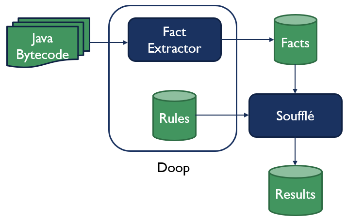
Figure 5. The Doop architecture.

To illustrate and evaluate the Datalog lifting approach outlined in Sec. 3, we modified the Doop (Bravenboer and Smaragdakis, 2009) Datalog-based pointer analysis framework , together with its underlying Soufflé (Jordan et al., 2016) Datalog engine . Fig. 5 outlines the Doop architecture. Doop is an extensible family of pointer and taint analyses implemented as Datalog rules. In addition, it includes a fact extractor from Java bytecode. Doop users select a particular analysis among the available analyses through a command-line argument. The rules corresponding to the chosen analysis (the IDB), together with the extracted facts (the EDB), are then passed to Soufflé.

⬇

New("o1", "A") @ True. // line 5

New("o2", "B") @ True. // line 6

Assign("o3", "o1") @ FA. // line 8

Assign("o3", "o2") @ !FA. // line 10

Store("o2", "f", "o1") @ FB. // line 13

Store("o2", "f", "o2") @ !FB. // line 15

Load("r", "o3", "f") @ True. // line 17

Figure 6. Annotated facts extracted from Listing 1.

Since Doop extracts syntactic facts, we need to identify the PCs of each of the syntactic tokens contributing to a fact, and associate the conjunction of those PCs as the fact PC. We had to do this for each type of fact extracted by Doop. The fact PC is just added to a fact as a trailing PC field, prefixed with ’@’. Facts with no PC field are assumed to belong to all products (an implicit PC of True ).

Our Doop modifications were only in the fact extractor. None of the Doop Datalog rules were changed. Our fact extraction modifications were scattered because extractors for different kinds of facts are implemented separately in Doop. However, all those changes were systematic and non-invasive. In total we modified only about 100 lines of code in the Doop fact extractor.

4.2. Lifting Soufflé

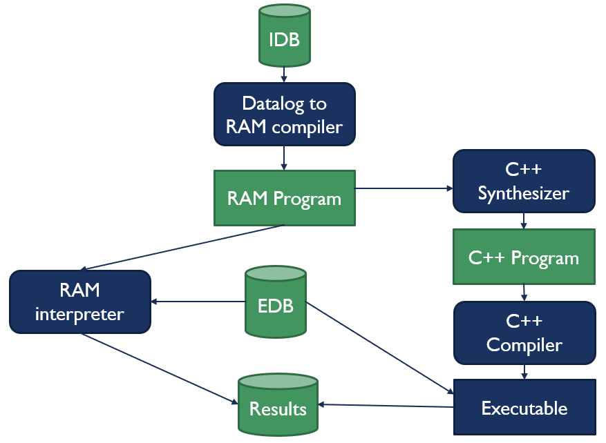
Figure 7. Soufflé architecture.

As seen in Fig. 7, a Soufflé program is first parsed and translated into a Relational Algebra Machine (RAM) program. RAM is a language with relational algebra constructs, in addition to a fixed-point looping operator. Based on a command-line argument, Soufflé then either interprets the RAM program on the fly, or synthesizes C++ code that is semantically equivalent to the RAM program. Since C++ programs are compiled (typically by optimizing compilers) into native machine code, native executables are at least an order of magnitude faster than interpreted analyses (Jordan et al., 2016). In this paper, we only cover the Soufflé interpreter.

At the syntax level, we extend the Soufflé language with fact annotations. Those are propositional formulas prefixed with ’@’. The Soufflé parser is extended with a syntactic category for propositional formulas. AST nodes for facts are extended with a PC field, with a default value of True. Propositional variables are added to a symbol table separate from that holding Soufflé identifiers.

As a part of compiling Soufflé programs into RAM, we turn syntactic presence conditions into Binary Decision Diagrams (BDDs). We use CUDD (Somenzi, 1998) as a BDD engine, and on top of it maintain a map from textual presence conditions to their corresponding canonical BDDs. As stated in $\mathrm{\widehat{infer}}$, when facts are resolved with a rule, the conjunction of their PCs becomes the conclusion’s PC.

Soufflé implements several indexing and query optimization techniques to improve inference time. To keep our changes independent of those optimizations, we add the presence condition as a field opaque to the query engine. We only manipulate this field as a PC when performing clause resolution, which takes place at a higher level than the details of indexing and query processing. This way we avoid touching relatively complex optimization code, while preserving the semantics of our lifted inference algorithm.

Some relational features of Soufflé were not lifted. For example, aggregation functions (sum, average, max, min, etc…) still return singleton values. None of those functions is used by Doop on lifted facts, so this does not affect the correctness of our results. We still plan to address this general limitation in the future though.

5. Evaluation

Table 1. Java product lines used for evaluation.

Benchmark	Size (KLOC)	Features	Valid Configurations
BerkeleyDB	70	42	8,759,844,864
GPL	1.4	21	4,176
Lampiro	45	18	2,048
MM08	5.7	27	784
Prevayler	7.9	5	32

We evaluate the performance of our lifted version of Doop (together with lifted Soufflé) on five Java benchmark product lines (previously used in the evaluation of other lifted analyses (Brabrand et al., 2012; Bodden et al., 2013)). For each of the benchmarks, Table 1 lists its size (in thousands of lines of code), number of features, and number of valid configurations according to its feature model. For example, BerkeleyDB is about 70,000 lines of code, comprised of 42 features, and has about 8.76 billion valid product configurations. We evaluate three Doop analyses: context-insensitive pointer analysis (insens), one-type heap-sensitive pointer analysis (1Type+Heap), and one-call-site heap-sensitive taint analysis (Taint-1Call+Heap). For taint analysis, we use the default sources, sinks, transform and sanitization functions curated in Doop for the JDK and Android (Grech and Smaragdakis, 2017). All experiments were performed on a Quad-core Intel Core i7-6700 processor running at 3.4GHZ, with 16GB RAM and hyper-threading enabled, running 64-bit Ubuntu Linux (kernel version 4.15).

Pointer and taint analyses work on the whole program, including library dependencies. Since general-purpose libraries usually do not have any variability, the comparison between lifted and single-product analyses is independent of them. Moreover, time spent in analyzing library code, and space taken by their facts, might skew the overall results. We restrict our experiments to application code and direct dependencies only using the Doop command-line argument "--Xfacts-subset APP_N_DEPS".

Doop extracts its facts from Java byte-code. However, SPL annotation techniques work at the source-code level. Feature selection usually takes place at compile-time, which means an SPL codebase is compiled into a single product. To get around this limitation, we had to choose benchmarks that only have disciplined annotations (Kästner et al., 2009), in the sense that adding or removing an annotation preserves the syntactic correctness of the 150% representation. This is not a limitation of our lifted inference algorithm though.

The benchmarks we chose are annotated using CIDE (Kästner et al., 2009), which uses different highlighting colors as presence conditions. We had to extract this color information from CIDE, together with the mapping from colors to locations of tokens (line and column number) in source files. Our fact extractor uses byte-code symbol information to locate tokens, and assign their presence conditions based on CIDE colors.

The primary goal of our experiments is to compare the performance of lifted analyses applied to the SPLs to that of running the corresponding product-level analyses on each of the valid configurations individually. Since the number of valid product configurations for some benchmarks is relatively big, it is neither practical nor particularly useful to enumerate all of the valid products and analyze them. Instead, for each SPL, we run the product-level analysis on two code-base subsets: the base code common across all variants, and the 150% representation (the whole SPL code-base, implementing all feature behaviors). Although those two extremes are not necessarily valid products, they are the lower bound and the upper bound in terms of code size, and averaging over them gives an "average" valid product approximation. The expected brute-force performance is the average valid product performance (P-Avg) multiplied by the number of valid configurations.

We split our evaluation into two parts: fact extraction and inference, and evaluate performance in terms of both the processing time and space (size of the fact database in kilobytes(KB)). Our primary research questions are:

RQ1: How do fact extraction time (and size of the extracted fact database) of lifted analyses compare to brute-force fact extraction?

RQ2: How do the Soufflé  inference time, and the size of the inferred database, of lifted analyses compare to brute-force analysis?

5.1. Fact Extraction

Table 2. Fact extraction time (in ms) and DB size (in KB): Average Product (P-Avg) vs SPL for all three analyses.

	insens				1Type+Heap				Taint-1Call+Heap
	Time(ms)		DB(KB)		Time(ms)		DB(KB)		Time(ms)		DB(KB)
	P-Avg	SPL	P-Avg	SPL	P-Avg	SPL	P-Avg	SPL	P-Avg	SPL	P-Avg	SPL
BerkeleyDB	5,136	4,541	31,892	49,725	4,651	4,809	71,536	122,922	4,647	4,667	64,497	112,060
GPL	816	814	175	409	782	876	245	593	789	802	188	462
Lampiro	4,413	4,475	41,100	41,170	4,425	4,145	149,521	149,686	4,237	4,436	230,035	230,370
MM08	1,226	1,364	1,921	3,259	1,250	1,372	3,878	6,990	1,255	1,252	4,234	7,829
Prevayler	1,416	1,554	3,230	4,407	1,453	1,454	5,882	8,630	1,502	1,404	3,917	5,534

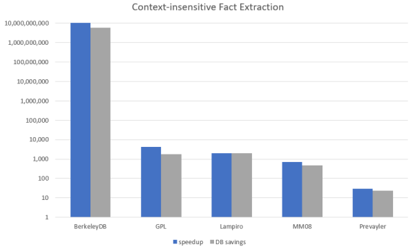
Figure 8. Context-insensitive Fact extraction speedup and DB savings factors: SPL vs average product.

Table 2 summarizes the "average" performance of product-level fact extraction (P-Avg) and that of the lifted fact extraction for the entire product line (SPL). For each of the three analyses, we compare fact extraction time (in milliseconds) and the size of the extracted database (in KB). For example, for context-insensitive analysis, average fact extraction time of a single product of Prevayler is 1,416ms, and the average size of the extracted fact database is 3,230KB. On the other hand, extracting facts from the whole Prevayler SPL at once takes 1,554ms, and the extracted fact database is 4,407KB. The difference between P-Avg Time and SPL Time is very small for all three analyses and five benchmarks, which is expected since extraction is syntactic and thus its time is proportional to code-base size, not the number of features. Size of the extracted database is noticeably bigger for lifted extraction (DB SPL columns) because lifted facts are augmented with presence conditions.

To evaluate the savings attributed to lifted fact extraction compared to brute-force extraction in terms of time and space, we compute the speedup and space saving factors (P-Avg * $|\operatorname{Conf}(\mathcal{L})|$ / SPL). Fig. 8 shows a log-scale bar graph of lifted fact extraction speedup and space savings for context-insensitive analysis. The other two analyses exhibit a similar trend and are omitted here. The figure shows that the time and space savings are proportional to the number of valid configurations of the product line. For example, Lampiro has 2048 valid configurations, and its lifted fact extraction is 2020 times faster than brute-force, with a database 2045 times smaller than the total space of brute-force databases. On the other hand, Prevayler has only 32 valid configurations, with an insens lifting speedup factor of 29, and a space savings factor of 23. Since different analyses typically require different facts, the size of the fact database also varies from one analysis to another. Experimental results do not show a direct correlation between an analysis and the size of its fact database. For example, in Lampiro, the Taint-1Call+Heap databases are significantly bigger than those of 1Type+Heap. BerkeleyDB, on the other hand, exhibits the opposite trend.

5.2. Inference

Table 3. Inference time (in ms) and inferred DB size (in KB): Average Product (P-Avg) vs SPL for the three analyses.

	insens				1Type+Heap				Taint-1Call+Heap
	Time(ms)		DB(KB)		Time(ms)		DB(KB)		Time(ms)		DB(KB)
	P-Avg	SPL	P-Avg	SPL	P-Avg	SPL	P-Avg	SPL	P-Avg	SPL	P-Avg	SPL
BerkeleyDB	9,184	10,810	141,728	200,655	13,598	17,273	318,349	483,206	17,479	21,474	285,473	443,737
GPL	4,422	4,517	2,033	3,528	4,794	4,718	3,237	5,675	8,999	8,861	2,500	4,450
Lampiro	8,264	8,111	245,933	246,285	21,372	20,725	980,689	981,549	44,365	45,996	1,393,038	1,394,826
MM08	4,596	4,720	8,788	13,021	5,106	5,142	19,058	29,453	9,340	9,306	18,302	29,383
Prevayler	4,908	5,334	15,856	19,808	5,852	6,013	29,605	38,747	9,785	9,717	20,611	26,279

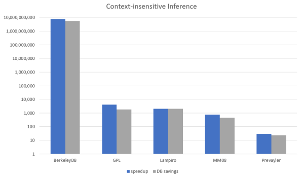
Figure 9. Context-insensitive Inference speedup and DB savings factors: SPL vs average product.

Table 3 summarizes the performance of lifted analyses on the entire product line (SPL) and that of product-level analyses on an average product (P-Avg). For example, running 1Type+Heap on an average MM08 product, inference is estimated to take 4,596ms, resulting in a database of 8,788KB. Running the same analysis on the whole MM08 product line though takes 8,788ms, resulting in a 13,021KB database. Fig. 9 is a log-scale bar graph of the speedup factor and the DB space savings factor for insens. Speedup and space savings trends are again proportional to the number of valid configurations. For example, for BerkeleyDB, lifted insens is about 7.4 billion times faster than brute-force, with a DB 5.6 billion times smaller. All three analyses show similar speedup and disk space savings trends.

Recall that the theoretic bottleneck of the lifted inference algorithm (Algorithm 2) is the satisfiability checks performed when conjoining two PCs. Since propositional satisfiability is NP-complete, we wanted to evaluate whether it is a bottleneck in practice. While SAT checks are not required to maintain correctness of the lifted inference algorithm, we perform them in order to avoid generating spurious facts that do not exist in any product. An UNSAT presence condition denotes an empty set of products, but what about PCs denoting sets of invalid product configurations? The Feature Model (FM) of a product line specifies which product configurations are valid and which are not. If a fact belongs only to a set of configurations excluded by the FM, then this fact can be removed. Removing spurious facts saves DB space, but, more importantly, keeps the set of facts searched by the inference algorithm as small as possible, improving the overall performance. We study the impact of SAT checking and using the FM below.

Table 4. SAT vs. noSAT. Time in milliseconds, Inferred DB in KB.

	insens				1Type+Heap				Taint-1Call+Heap
	Time(ms)		DB(KB)		Time(ms)		DB(KB)		Time(ms)		DB(KB)
	SPL	noSAT	SPL	noSAT	SPL	noSAT	SPL	noSAT	SPL	noSAT	SPL	noSAT
BerkeleyDB	10,810	10,879	49,725	53,151	17,273	17,784	122,922	143,720	21,474	21,920	112,060	128,427
GPL	4,517	4,496	409	472	4,718	4,667	593	765	8,861	8,812	462	595
Lampiro	8,111	8,105	41,170	41,170	20,725	21,224	149,686	149,710	45,996	47,132	230,370	230,370
MM08	4,720	4,689	3,259	3,762	5,142	5,118	6,990	8,775	9,306	9,270	7,829	9,082
Prevayler	5,334	5,050	4,407	4,638	6,013	5,940	8,630	9,392	9,717	9,903	5,534	5,869

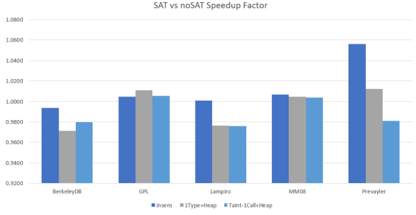
Figure 10. Inference time: SPL vs. SPL with SAT checking disabled for all three analyses.

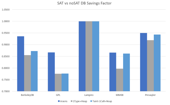
Figure 11. Inferred database size (KB): SPL vs. SPL with SAT checking disabled for all three analyses.

RQ2.1: How much does SAT checking contribute to the processing time of the lifted Datalog engine?

Table 4 summarizes the performance of our lifted analyses and the same analyses with SAT checking disabled (noSAT). Fig. 10 and Fig. 11 show the noSAT-associated speedup and database size savings, respectively. Recall that we represent PCs using BDDs. SAT checking over BDDs is a constant-time operation (Huth and Ryan, 2004). Since conjoining and disjoining BDDs can take exponential time, we disable all BDD operations, keeping only the textual representation of PCs. A speedup factor below 1.0 means that disabling SAT checks slows down inference. This is what we observed for most of the benchmarks. We believe that the slowdown is because of the use of textual representation of PCs which resulted in a much bigger PC table, with slower lookup times. We also do not see any DB savings because non-canonically represented PCs tend to be longer than BDD-based ones, resulting, on average, in more characters (and bytes) per PC. We note that the number of features is relatively low in all of our benchmarks. BDD-based SAT solving is known to perform well on such small number of propositional variables. With product lines of hundreds or thousands of features, it is possible that noSAT might result in performance improvements.

Table 5. SPL vs. SPL+FM. Time in milliseconds, Inferred DB in KB.

	insens				1Type+Heap				Taint-1Call+Heap
	Time(ms)		DB(KB)		Time(ms)		DB(KB)		Time(ms)		DB(KB)
	SPL	SPL+FM	SPL	SPL+FM	SPL	SPL+FM	SPL	SPL+FM	SPL	SPL+FM	SPL	SPL+FM
BerkeleyDB	10,810	11,693	49,725	721,927	17,273	22,276	122,922	1,859,320	21,474	24,140	112,060	1,625,278
GPL	4,517	4,587	409	9,447	4,718	4,728	593	13,809	8,861	8,918	462	10,644
Lampiro	8,111	8,528	41,170	325,848	20,725	22,283	149,686	1,283,639	45,996	48,688	230,370	1,843,151
MM08	4,720	4,761	3,259	69,017	5,142	5,288	6,990	158,732	9,306	9,476	7,829	158,330
Prevayler	5,334	5,169	4,407	8,825	6,013	5,984	8,630	17,564	9,717	9,977	5,534	11,394

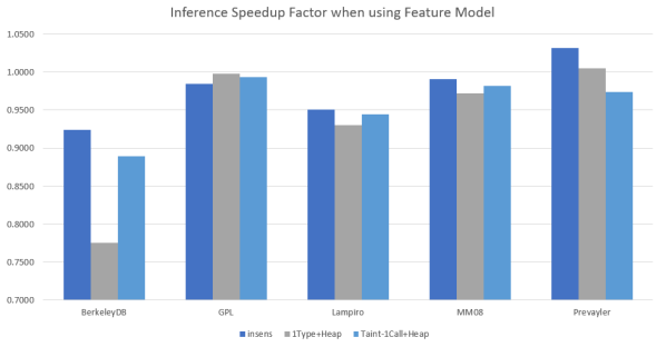
Figure 12. Inference time: SPL vs. SPL with FM for all three analyses.

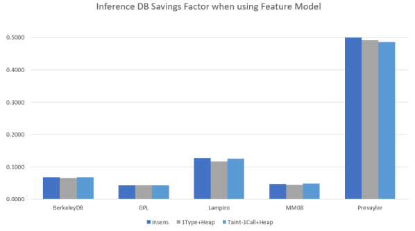
Figure 13. Inferred database size (KB): SPL vs. SPL with FM for all three analyses.

Table 6. The number of inferred facts with and without the Feature Model (FM).

	insens		1Type+Heap		Taint-1Call+Heap
	SPL	SPL+FM	SPL	SPL+FM	SPL	SPL+FM
BerkeleyDB	200,655	200,650	483,206	483,201	443,737	443,732
GPL	3,528	3,128	5,675	4,821	4,450	3,800
Lampiro	246,285	246,221	981,549	980,823	1,394,826	1,394,825
MM08	13,021	13,021	29,453	29,452	29,383	29,381
Prevayler	19,808	19,808	38,747	38,747	26,279	26,279

RQ2.2: What is the effect of taking the feature model (FM) of an SPL into consideration when running Datalog variability-aware analyses, in terms of inference time and DB size?

Table 5 compares the performance of our lifted analyses against the same analyses using the feature model (SAT+FM). SAT+FM entails conjoining the feature model to each PC before performing the satisfiability check. If the PC encodes a set of products excluded by the FM, the conjunction is unsatisfiable. Fig. 12 and Fig. 13 show the SAT+FM-associated speedup and space savings, respectively. For most of the experiments, using the FM results in slowdowns and larger DBs. FM usage reduces the number of inferred facts, as observed in Table 6, but the reduction is relatively small. On the other hand, PCs now conjoined with the FM are more complex, taking longer to construct (hence the performance penalty), and more bytes to store (hence the bigger DBs).

5.3. Threats to Validity

For internal threats, we note that all of our benchmarks are CIDE product lines. While our lifting approach and implementation are not specific to CIDE, CIDE limitations make the benchmarks biased towards specific annotation patterns. For example, only well-behaved annotations are allowed. Furthermore, since feature expressions do not support feature negation, all input PCs are satisfiable, as well as conjunctions over those PCs. We experimented with disabling satisfiability checks to see how much they affect performance (while they always return true for this set of benchmarks). As noted previously, the overhead of those checks is marginal.

Another internal threat is that we approximate average product performance using only two samples (the maximum and the minimum). These averages are not expected to be completely accurate, but are used to give a brute-force estimate. Our experiments show performance improvement of several orders of magnitude, so we believe that our approximation (compared to more elaborate configuration sampling techniques) can be tolerated.

Finally, all of the the analyses we used come from the Doop framework. Again, nothing in our lifted inference engine is Doop-specific, but extraction of annotated features is a part of Doop. Other frameworks can extract fact annotations in a similar fashion.

6. Related Work

Different kinds of software analyses have been re-implemented to support product lines (Thüm et al., 2014). For example, the TypeChef project (Kästner et al., 2011, 2012) implements variability aware parsers (Kästner et al., 2011) and type checkers (Kästner et al., 2012) for Java and C. The SuperC project (Gazzillo and Grimm, 2012) is another C language variability-aware parser. The Henshin (Arendt et al., 2010) graph transformation engine was lifted to support product lines of graphs (Salay et al., 2014). Those lifted analyses were written from scratch, without reusing any components from their respective product-level analyses. Our approach, on the other hand, lifts an entire class of product-level analyses written as Datalog rules, by lifting their inference engine (and extracting presence conditions together with facts).

SPL^Lift (Bodden et al., 2013) extends IFDS (Reps et al., 1995) data flow analyses to product lines. Model checkers based on Featured Transition Systems (Classen et al., 2013) check temporal properties of transition systems where transitions can be labeled by presence conditions. Both of these SPL analyses use almost the same single-product analyses on a lifted data representation. At a high level, our approach is similar in the sense that the logic of the original analysis is preserved, and only data is augmented with presence conditions. Still, our approach is unique because we do not touch any of the Datalog rules comprising the analysis logic itself.

Syntactic transformation techniques have been suggested for lifting abstract interpretation analyses to SPLs (Midtgaard et al., 2015). This line of work outlines a systematic approach to lifting abstract interpretation analyses, together with correctness proofs. Yet this approach is not automated which means lifted analyses still need to be written from scratch, albeit while being guided by some systematic guidelines.

Datalog engines have been used as backends by several program analysis frameworks. In addition to Doop, examples of analysis frameworks based on logic programming include XSB (Dawson et al., 1996), bddbddb (Whaley et al., 2005) and Paddle (Lhoták and Hendren, 2008). DIMPLE (Benton and Fischer, 2007) is another declarative pointer analysis framework where rules are written in Prolog. To the best of our knowledge, all those program analysis frameworks have been targeting single products. Our primary contribution is lifting this class of analyses to SPLs in a generic way, without making any analysis-specific assumptions. In addition, our approach can be systematically implemented in any Datalog engine used by any of those frameworks.

7. Conclusion

In this paper, presented an algorithm for lifting Datalog-based software analyses to SPLs. We implemented this algorithm in the Soufflé Datalog engine, and evaluated performance of three program analyses from the Doop framework on a suite of SPL benchmarks. Comparing our lifted implementation to brute-force analysis of each product individually, we show significant savings in terms of processing time and database size.

Our Soufflé implementation only lifts the interpreter but not the code generator (compiler). Aggregation functions (e.g., sum, count) are not currently lifted either. We plan to address these implementation level limitations in future work. We also plan to evaluate lifted Soufflé on analyses frameworks other than Doop. Another track for future work is lifting Datalog rules, not just facts. This would allow us to apply a product line of analyses to an SPL all at once. Our work can also be extended to lift Horn-Clause based analysis and verification tools (Bjørner et al., 2015) to support SPLs.

References

- (1)
- Arendt et al. (2010) Thorsten Arendt, Enrico Biermann, Stefan Jurack, Christian Krause, and Gabriele Taentzer. 2010. Henshin: Advanced Concepts and Tools for In-place EMF Model Transformations. In Proceedings of the 13th International Conference on Model Driven Engineering Languages and Systems: Part I (MODELS’10). Springer-Verlag, Berlin, Heidelberg, 121–135. http://dl.acm.org/citation.cfm?id=1926458.1926471
- Benton and Fischer (2007) William C. Benton and Charles N. Fischer. 2007. Interactive, Scalable, Declarative Program Analysis: From Prototype to Implementation. In Proceedings of the 9th ACM SIGPLAN International Conference on Principles and Practice of Declarative Programming (PPDP ’07). ACM, New York, NY, USA, 13–24. https://doi.org/10.1145/1273920.1273923
- Bjørner et al. (2015) Nikolaj Bjørner, Arie Gurfinkel, Ken McMillan, and Andrey Rybalchenko. 2015. Horn Clause Solvers for Program Verification. Springer International Publishing, Cham, 24–51. https://doi.org/10.1007/978-3-319-23534-9_2
- Bodden et al. (2013) Eric Bodden, Társis Tolêdo, Márcio Ribeiro, Claus Brabrand, Paulo Borba, and Mira Mezini. 2013. SPLLIFT: Statically Analyzing Software Product Lines in Minutes Instead of Years. In Proceedings of the 34th ACM SIGPLAN Conference on Programming Language Design and Implementation (PLDI ’13). ACM, New York, NY, USA, 355–364. https://doi.org/10.1145/2491956.2491976
- Brabrand et al. (2012) Claus Brabrand, Márcio Ribeiro, Társis Tolêdo, and Paulo Borba. 2012. Intraprocedural Dataflow Analysis for Software Product Lines. In Proceedings of the 11th Annual International Conference on Aspect-oriented Software Development (AOSD ’12). ACM, New York, NY, USA, 13–24. https://doi.org/10.1145/2162049.2162052
- Bravenboer and Smaragdakis (2009) Martin Bravenboer and Yannis Smaragdakis. 2009. Strictly Declarative Specification of Sophisticated Points-to Analyses. In Proceedings of the 24th ACM SIGPLAN Conference on Object Oriented Programming Systems Languages and Applications (OOPSLA ’09). ACM, New York, NY, USA, 243–262. https://doi.org/10.1145/1640089.1640108
- Ceri et al. (1989) S. Ceri, G. Gottlob, and L. Tanca. 1989. What you always wanted to know about Datalog (and never dared to ask). IEEE Transactions on Knowledge and Data Engineering 1, 1 (March 1989), 146–166. https://doi.org/10.1109/69.43410
- Classen et al. (2013) Andreas Classen, Maxime Cordy, Pierre-Yves Schobbens, Patrick Heymans, Axel Legay, and Jean-Francois Raskin. 2013. Featured Transition Systems: Foundations for Verifying Variability-Intensive Systems and Their Application to LTL Model Checking. IEEE Trans. Softw. Eng. 39, 8 (Aug. 2013), 1069–1089. https://doi.org/10.1109/TSE.2012.86
- Classen et al. (2010) Andreas Classen, Patrick Heymans, Pierre-Yves Schobbens, Axel Legay, and Jean-François Raskin. 2010. Model Checking Lots of Systems: Efficient Verification of Temporal Properties in Software Product Lines. In Proceedings of the 32Nd ACM/IEEE International Conference on Software Engineering - Volume 1 (ICSE ’10). ACM, New York, NY, USA, 335–344. https://doi.org/10.1145/1806799.1806850
- Dawson et al. (1996) Steven Dawson, C. R. Ramakrishnan, and David S. Warren. 1996. Practical Program Analysis Using General Purpose Logic Programming Systems&Mdash;a Case Study. In Proceedings of the ACM SIGPLAN 1996 Conference on Programming Language Design and Implementation (PLDI ’96). ACM, New York, NY, USA, 117–126. https://doi.org/10.1145/231379.231399
- Gazzillo and Grimm (2012) Paul Gazzillo and Robert Grimm. 2012. SuperC: Parsing All of C by Taming the Preprocessor. In Proceedings of the 33rd ACM SIGPLAN Conference on Programming Language Design and Implementation (PLDI ’12). ACM, New York, NY, USA, 323–334. https://doi.org/10.1145/2254064.2254103
- Grech and Smaragdakis (2017) Neville Grech and Yannis Smaragdakis. 2017. P/Taint: Unified Points-to and Taint Analysis. Proc. ACM Program. Lang. 1, OOPSLA, Article 102 (Oct. 2017), 28 pages. https://doi.org/10.1145/3133926
- Greco and Molinaro (2016) Sergio Greco and Cristian Molinaro. 2016. Datalog and Logic Databases. Morgan & Claypool.
- Huth and Ryan (2004) Michael Huth and Mark Ryan. 2004. Logic in Computer Science (2nd ed.). Cambridge University Press.
- Jordan et al. (2016) Herbert Jordan, Bernhard Scholz, and Pavle Subotić. 2016. Soufflé: On Synthesis of Program Analyzers. In Computer Aided Verification, Swarat Chaudhuri and Azadeh Farzan (Eds.). Springer International Publishing, Cham, 422–430.
- Kästner et al. (2012) Christian Kästner, Sven Apel, Thomas Thüm, and Gunter Saake. 2012. Type Checking Annotation-based Product Lines. ACM Trans. Softw. Eng. Methodol. 21, 3, Article 14 (July 2012), 39 pages. https://doi.org/10.1145/2211616.2211617
- Kästner et al. (2009) Christian Kästner, Sven Apel, Salvador Trujillo, Martin Kuhlemann, and Don Batory. 2009. Guaranteeing Syntactic Correctness for All Product Line Variants: A Language-Independent Approach. In Objects, Components, Models and Patterns, Manuel Oriol and Bertrand Meyer (Eds.). Springer Berlin Heidelberg, Berlin, Heidelberg, 175–194.
- Kästner et al. (2011) Christian Kästner, Paolo G. Giarrusso, Tillmann Rendel, Sebastian Erdweg, Klaus Ostermann, and Thorsten Berger. 2011. Variability-aware Parsing in the Presence of Lexical Macros and Conditional Compilation. In Proceedings of the 2011 ACM International Conference on Object Oriented Programming Systems Languages and Applications (OOPSLA ’11). ACM, New York, NY, USA, 805–824. https://doi.org/10.1145/2048066.2048128
- Lhoták and Hendren (2008) Ondřej Lhoták and Laurie Hendren. 2008. Evaluating the Benefits of Context-sensitive Points-to Analysis Using a BDD-based Implementation. ACM Trans. Softw. Eng. Methodol. 18, 1, Article 3 (Oct. 2008), 53 pages. https://doi.org/10.1145/1391984.1391987
- Liebig et al. (2013) Jörg Liebig, Alexander von Rhein, Christian Kästner, Sven Apel, Jens Dörre, and Christian Lengauer. 2013. Scalable Analysis of Variable Software. In Proceedings of the 2013 9th Joint Meeting on Foundations of Software Engineering (ESEC/FSE 2013). ACM, New York, NY, USA, 81–91. https://doi.org/10.1145/2491411.2491437
- Madsen et al. (2016) Magnus Madsen, Ming-Ho Yee, and Ondřej Lhoták. 2016. From Datalog to Flix: A Declarative Language for Fixed Points on Lattices. In Proceedings of the 37th ACM SIGPLAN Conference on Programming Language Design and Implementation (PLDI ’16). ACM, New York, NY, USA, 194–208. https://doi.org/10.1145/2908080.2908096
- Midtgaard et al. (2015) Jan Midtgaard, Aleksandar S. Dimovski, Claus Brabrand, and Andrzej Wąsowski. 2015. Systematic Derivation of Correct Variability-aware Program Analyses. Sci. Comput. Program. 105, C (July 2015), 145–170. https://doi.org/10.1016/j.scico.2015.04.005
- Reps et al. (1995) Thomas Reps, Susan Horwitz, and Mooly Sagiv. 1995. Precise Interprocedural Dataflow Analysis via Graph Reachability. In Proceedings of the 22Nd ACM SIGPLAN-SIGACT Symposium on Principles of Programming Languages (POPL ’95). ACM, New York, NY, USA, 49–61. https://doi.org/10.1145/199448.199462
- Salay et al. (2014) Rick Salay, Michalis Famelis, Julia Rubin, Alessio Di Sandro, and Marsha Chechik. 2014. Lifting Model Transformations to Product Lines. In Proceedings of the 36th International Conference on Software Engineering (ICSE 2014). ACM, New York, NY, USA, 117–128. https://doi.org/10.1145/2568225.2568267
- Smaragdakis and Balatsouras (2015) Yannis Smaragdakis and George Balatsouras. 2015. Pointer Analysis. Foundations and Trends in Programming Languages 2, 1 (2015), 1–69. https://doi.org/10.1561/2500000014
- Somenzi (1998) Fabio Somenzi. 1998. CUDD: CU Decision Diagram Package Release 2.2.0. (06 1998).
- Thüm et al. (2014) Thomas Thüm, Sven Apel, Christian Kästner, Ina Schaefer, and Gunter Saake. 2014. A Classification and Survey of Analysis Strategies for Software Product Lines. ACM Comput. Surv. 47, 1, Article 6 (June 2014), 45 pages. https://doi.org/10.1145/2580950
- Whaley et al. (2005) John Whaley, Dzintars Avots, Michael Carbin, and Monica S. Lam. 2005. Using Datalog with Binary Decision Diagrams for Program Analysis. In Proceedings of the Third Asian Conference on Programming Languages and Systems (APLAS’05). Springer-Verlag, Berlin, Heidelberg, 97–118. https://doi.org/10.1007/11575467_8