Learning Blended, Precise Semantic Program Embeddings

Abstract.

Learning neural program embeddings is key to utilizing deep neural networks in program languages research — precise and efficient program representations enable the application of deep models to a wide range of program analysis tasks. Existing approaches predominately learn to embed programs from their source code, and, as a result, they do not capture deep, precise program semantics. On the other hand, models learned from runtime information critically depend on the quality of program executions, thus leading to trained models with highly variant quality. This paper tackles these inherent weaknesses of prior approaches by introducing a new deep neural network, LiGer, which learns program representations from a mixture of symbolic and concrete execution traces. We have evaluated LiGer on COSET, a recently proposed benchmark suite for evaluating neural program embeddings. Results show LiGer (1) is significantly more accurate than the state-of-the-art syntax-based models Gated Graph Neural Network and code2vec in classifying program semantics, and (2) requires on average 10x fewer executions covering 74% fewer paths than the state-of-the-art dynamic model DYPRO. Furthermore, we extend LiGer to predict the name for a method from its body’s vector representation. Learning on the same set of functions (more than 170K in total), LiGer significantly outperforms code2seq, the previous state-of-the-art for method name prediction.

1. Introduction

Learning representations has been a major focus in deep learning research for the past several years. Mikolov et al. pioneered the field with their seminal work on learning word embeddings (Mikolov et al., 2013b; Mikolov et al., 2013a). The idea is to construct a vector space for a corpus of text such that words found in similar contexts in the corpus are located in close proximity to one another in the vector space. Word embeddings, along with other representation learning (e.g. doc2vec (Le and Mikolov, 2014)), become vital in solving many downstream Natural Language Processing (NLP) tasks such as language modeling (Bengio et al., 2003) and sentiment classification (Glorot et al., 2011).

Similar to word embeddings, the goal of this paper is to learn program embeddings, vector representations of program semantics. By learning program embeddings, the power of deep neural networks (DNNs) can be utilized to tackle many program analysis tasks. For example, Alon et al. (2019) presents a DNN to predict the name of a method given its body. Wang et al. (2017) propose a deep model to guide the repair of student programs in Massive Open Online Courses (MOOCs). Despite such notable advances, an important challenge remains: How to tackle the precision and efficiency issues in learning program embeddings? As illustrated by Wang and Christodorescu (2019), due to the inherent gap between program syntax and semantics, models learned from source code (i.e., the static models) can be imprecise at capturing semantic properties. Consider for example the programs in Figure 1. State-of-the-art static models can neither recognize the equivalent semantics between programs in Figures 1 and 1(a), nor the different semantics between programs in Figures 1 and 1. The reason for this is quite obvious — static models base their predictions on the surface-level program syntax. Specifically, programs 1 and 1 are syntactically much more similar than programs 1 and 1(a) despite that programs 1 and 1(a) implement the same sorting strategy, namely Bubble Sort.

⬇

static int SortI(int[] A)

{

int left = 0;

int right = ;

for(int i= ) {

for(int j= ) {

if (A[j] > A[j + 1]) {

int tmp = A[j];

A[j] = A[j + 1];

A[j + 1] = tmp;

}}}

return A;

}

Listing 1: Bubble Sort

⬇

static int SortII(int[] A)

{

int left = 0;

int right = left@;i@<right@;i@++ i-1 ) {

if (A[j] > A[j + 1]) {

int tmp = A[j];

A[j] = A[j + 1];

A[j + 1] = tmp;

}}}

return A;

}

Listing 2: Insertion Sort

⬇

static int SortIII(int[] A)

{

int swappbit = 1;

while (swappbit != 0) {

swappbit = 0;

for (int i=0;i<A.Length-1;i++)

{

if (A[i + 1] > A[i]) {

int tmp = A[i];

A[i] = A[i + 1];

A[i + 1] = tmp;

swappbit = 1;

}}}

return A;

}

(a) Bubble Sort

Listing 3: Example programs that implement a sorting routine. Code highlighted within the shadow boxes depicts the syntactic differences between programs 1 and 1.

⬇

$\{$A:[8, 5, 1, 4, 3]; left:0; right:$\bot$$\}$

$\{$A:[8, 5, 1, 4, 3]; left:0; right:4$\}$

$\{$A:[5, 5, 1, 4, 3]; left:0; right:4$\}$

$\{$A:[5, 8, 1, 4, 3]; left:0; right:4$\}$

$\{$A:[5, 1, 1, 4, 3]; left:0; right:4$\}$

$\{$A:[5, 1, 8, 4, 3]; left:0; right:4$\}$

$\{$A:[5, 1, 4, 4, 3]; left:0; right:4$\}$

$\{$A:[5, 1, 4, 8, 3]; left:0; right:4$\}$

$\{$A:[5, 1, 4, 3, 3]; left:0; right:4$\}$

$\{$A:[5, 1, 4, 3, 8]; left:0; right:4$\}$

$\{$A:[1, 1, 4, 3, 8]; left:0; right:4$\}$

$\{$A:[1, 5, 4, 3, 8]; left:0; right:4$\}$

$\{$A:[1, 4, 4, 3, 8]; left:0; right:4$\}$

$\{$A:[1, 4, 5, 3, 8]; left:0; right:4$\}$

$\{$A:[1, 4, 3, 3, 8]; left:0; right:4$\}$

$\{$A:[1, 4, 3, 5, 8]; left:0; right:4$\}$

$\{$A:[1, 3, 3, 5, 8]; left:0; right:4$\}$

$\{$A:[1, 3, 4, 5, 8]; left:0; right:4$\}$

(b)

⬇

$\{$A:[8, 5, 1, 4, 3]; left:0; right:$\bot$$\}$

$\{$A:[8, 5, 1, 4, 3]; left:0; right:5$\}$

$\{$A:[5, 5, 1, 4, 3]; left:0; right:5$\}$

$\{$A:[5, 8, 1, 4, 3]; left:0; right:5$\}$

$\{$A:[5, 1, 1, 4, 3]; left:0; right:5$\}$

$\{$A:[5, 1, 8, 4, 3]; left:0; right:5$\}$

$\{$A:[1, 1, 8, 4, 3]; left:0; right:5$\}$

$\{$A:[1, 5, 8, 4, 3]; left:0; right:5$\}$

$\{$A:[1, 5, 4, 4, 3]; left:0; right:5$\}$

$\{$A:[1, 5, 4, 8, 3]; left:0; right:5$\}$

$\{$A:[1, 4, 4, 8, 3]; left:0; right:5$\}$

$\{$A:[1, 4, 5, 8, 3]; left:0; right:5$\}$

$\{$A:[1, 4, 5, 3, 3]; left:0; right:5$\}$

$\{$A:[1, 4, 5, 3, 8]; left:0; right:5$\}$

$\{$A:[1, 4, 3, 3, 8]; left:0; right:5$\}$

$\{$A:[1, 4, 3, 5, 8]; left:0; right:5$\}$

$\{$A:[1, 3, 3, 5, 8]; left:0; right:5$\}$

$\{$A:[1, 3, 4, 5, 8]; left:0; right:5$\}$

(c)

⬇

$\{$A:[8, 5, 1, 4, 3]; swapbit:1$\}$

$\{$A:[8, 5, 1, 4, 3]; swapbit:0$\}$

$\{$A:[5, 5, 1, 4, 3]; swapbit:1$\}$

$\{$A:[5, 8, 1, 4, 3]; swapbit:1$\}$

$\{$A:[5, 1, 1, 4, 3]; swapbit:1$\}$

$\{$A:[5, 1, 8, 4, 3]; swapbit:1$\}$

$\{$A:[1, 1, 8, 4, 3]; swapbit:1$\}$

$\{$A:[1, 5, 8, 4, 3]; swapbit:1$\}$

$\{$A:[1, 5, 4, 4, 3]; swapbit:1$\}$

$\{$A:[1, 5, 4, 8, 3]; swapbit:1$\}$

$\{$A:[1, 4, 4, 8, 3]; swapbit:1$\}$

$\{$A:[1, 4, 5, 8, 3]; swapbit:1$\}$

$\{$A:[1, 4, 5, 3, 3]; swapbit:1$\}$

$\{$A:[1, 4, 5, 3, 8]; swapbit:1$\}$

$\{$A:[1, 4, 3, 3, 8]; swapbit:1$\}$

$\{$A:[1, 4, 3, 5, 8]; swapbit:1$\}$

$\{$A:[1, 3, 3, 5, 8]; swapbit:1$\}$

$\{$A:[1, 3, 4, 5, 8]; swapbit:1$\}$

(d)

Figure 1. Encoding the executions of the programs in Figure 1 with the input array A = [8,5,1,4,3]. At each step, the variable in bold is updated. Steps that are underlined illustrate the semantic differences between bubble sort (program 1) and insertion sort (program 1) concerning only the manipulation of the input array A. Note that we have omitted all loop induction variables, variable tmp in both programs 1 and 1 as well as some steps that update the variable swapbit in program 1(a) to simply our presentation.

In parallel, a separate class of models have been proposed that embed programs from their concrete execution traces (i.e., the dynamic models). Compared to source code, program executions capture accurate, deep program semantics, thus offering benefits beyond static models that reason over syntactic representations. Figure 1 shows the executions of the three programs with an input array A = [8,5,1,4,3] according to the state-based encoding proposed by Wang et al. (2017). Naturally, the semantic relationship among the three programs becomes much clearer. Despite their advantages, the performance of dynamic models heavily depends on the quality of program executions. In particular, dynamic models, similar to dynamic program analysis, can suffer from insufficient code coverage. Even for each covered path, dynamic models may need a large number of execution instances to generalize, resulting in a lengthy and expensive training process.

To tackle those aforementioned issues of both strands of prior work, we introduce a novel, blended approach for learning precise and efficient representations of program semantics. Our insight is to blend the respective strengths of static and dynamic models to mitigate their respective weaknesses. To this end, we propose a carefully designed blended model to learn a deep, precise semantic representation. Different from dynamic models that consider only program states created along an execution path, our blended model incorporates the additional symbolic representation of each statement (i.e. symbolic trace) whose execution leads to a corresponding program state.

The benefits of blending these feature dimensions are twofold. First, learning from symbolic program encodings is shown difficult for DNNs (Wang and Christodorescu, 2019; Wang, 2019). Concrete program states, which give live illustrations of program behavior, provide explanations to DNNs about each symbolic statement’s semantics. As a result, models trained on the combined features capture deeper semantic properties than symbolic traces alone (cf. Section 6.2.2). Second, a symbolic trace typically generalizes a large number of concrete executions. Therefore, symbolic traces present high-level, general descriptions of program meaning to DNNs. It is for this very reason that symbolic traces stand out as the major feature dimension from which models generalize. In the presence of the symbolic feature dimension, DNNs deemphasize the role of dynamic program features, leading to reduced demand on the number of concrete executions. As another benefit of our blended model, we observe that DNNs trained on both feature dimensions are also more resilient to the varying diversity on program executions. Indeed, when the path coverage on the targeted program is systematically reduced, our blended network largely maintains its accuracy, and thus has improved data reliance (cf. Section 6.1.3).

We have realized our approach in a new DNN, LiGer, and extensively evaluated it. Using COSET (Wang and Christodorescu, 2019), a recently proposed benchmark suite for evaluating neural program embeddings, we find LiGer achieves significantly better accuracy and stability than Gated Graph Neural Network (GGNN) (Allamanis et al., 2017) and code2vec (Alon et al., 2019), two of the most widely applied static models in their respective problem domains. Compared to DYPRO (Wang, 2019), the state-of-the-art dynamic model in learning program embeddings, LiGer is more accurate even when generalizing from on average almost 10x fewer executions that cover 74% fewer code paths per program.

We also extend LiGer to solve the method name prediction problem studied by Alon et al. (2019). Our dataset contains 174,922 functions extracted from logs of coding interviews conducted by an IT company for testing a candidate’s programming skills. Each function is written by a candidate to solve an algorithmic question (e.g., merging two sorted arrays, determining if a string is a palindrome, detecting the presence of a cycle in a linked list, etc.). All method names were provided by the interviewers for describing the functionality of each method. We strip away the method names for models to predict. Results show that LiGer significantly outperforms all competing deep neural architectures, including code2seq (Alon et al., 2018), the previous state-of-the-art.

We make the following main contributions:

• We propose a novel, blended approach that combines static and dynamic program features for learning precise and efficient representations of program semantics.

• We realize our approach in LiGer, which achieves significantly better accuracy and stability than GGNN and code2vec on COSET and requires far fewer program executions for both training and testing than DYPRO.

• We extend LiGer to solve the method name prediction problem. Results show that LiGer also significantly outperforms code2seq, the previous state-of-the-art DNN.

• We present the details of our extensive evaluation of LiGer, including an ablation study that analyzes the contributions of LiGer’s several crucial components to its overall performance.

2. Overview

This section overviews our blended approach of learning program embeddings. In particular, it explains how we address the deficiencies of static and dynamic models. We begin by formalizing the notion of execution traces and several pertinent concepts.

⬇

public bool isRotateString(string A,string B)

{

if (A.Length != B.Length)

return false;

for (int i = 1; i < A.Length; i++)

{

string tail=A.Substring(i,A.Length-i);

string wrap=A.Substring(0, i);

if (tail + wrap == B)

return true;

}

return false;

}

(e)

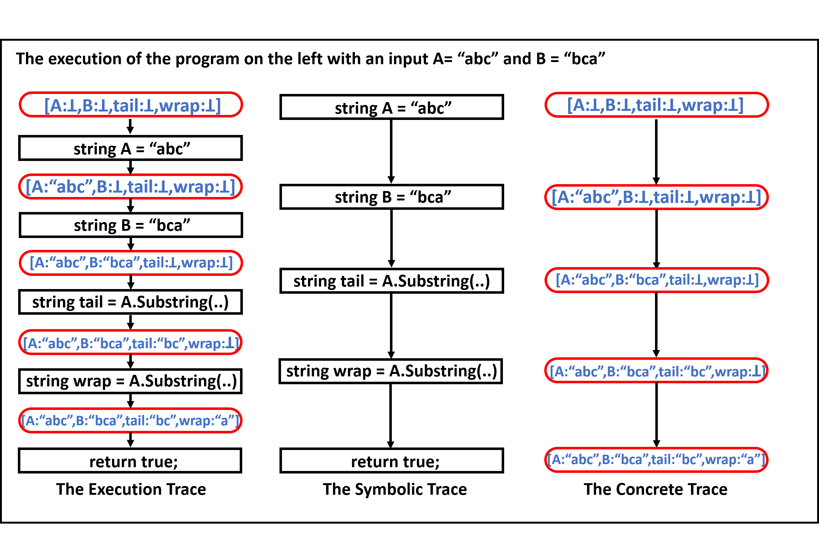
(f)

Figure 2. Given the program in (1(e)), we give example execution traces, symbolic traces and concrete traces in (1(f)).

2.1. Formalization

In general, given a program $P$ and an input $I$, an execution trace is obtained by executing $P$ on $I$. Its concept and notations are standard, which we formalize more precisely below.

Definition 2.0.

(Execution Trace) An execution trace, denoted by $\pi$, is a sequence in the form of $s_{0}\rightarrow(e_{i}\rightarrow s_{i})^{*}$, where $e_{i}$ denotes a statement encountered as $P$ executes on an input $I$; $s_{i}$ denotes a program state, which is a set of variable/memory and value pairs immediately after the execution of statement $e_{i}$; $s_{0}$ is the initial program state; and ^∗ denotes the Kleene star.

As an example, Figure 1(f) presents a graphical illustration of an execution trace of the program in Figure 1(e) with input A = "abc" and B = "bca".

Definition 2.0.

(Symbolic Trace) Given an execution trace, $\pi$, a symbolic trace, $\sigma$, is the sequence of statements visited in $\pi$ in the form of $(e_{i}\rightarrow e_{i+1})^{*}$.

Similarly, Figure 1(f) also gives an example symbolic trace, which is a projection of the execution trace w.r.t. the program statements.

Definition 2.0.

(State Trace) Given an execution trace, $\pi$, a state trace, $\epsilon$, is the sequence of program states created in $\pi$ in the form of $(s_{i}\rightarrow s_{i+1})^{*}$.

Again, Figure 1(f) shows an example state trace, which is a projection of the execution trace w.r.t. the program states.

2.2. Motivation and Insight

Learning program embeddings from execution traces has been explored in the literature. The prior work can be divided into two categories: static and dynamic. The former refers to learning program embeddings exclusively on symbolic traces. As an example, Henkel et al. (2018) train a model from symbolic traces for a code analogy task. Although learning from symbolic traces captures, to a certain degree, program properties more at the semantic level than purely the syntactic source code, it suffers from the same fundamental issue of all static models. That is such approaches leave the burden on the deep models to reason about program semantics through a syntactic representation, a task that is proven to be challenging even for state-of-the-art DNNs. To give a simple example, a capable neural network needs to recognize the identical semantics i+=i and i*=2 denote because such variations are ubiquitous in real-world code. Note that Henkel et al.’s approach relies on user-defined abstraction templates, which unfortunately do not address the problem’s root cause.

In contrast to the symbolic trace-based approaches, another line of work only considers concrete state traces for learning program representations. In particular, Wang et al. (2017) propose a model learned from concrete state traces to predict the type of errors students make in their programming assignments. The intuition behind the approach is to capture the semantics of a program through the states that are created in an execution. The advantage of their approach is the canonicalization of syntactic variations as programs of equivalent semantics will always create identical program states regardless of their syntactic differences (e.g., the earlier example involving i+=i and i*=2). Despite this strength, models that embed programs from concrete state traces have their own weaknesses. In principle, a symbolic trace can be instantiated to a large or arbitrary number of concrete states traces. Therefore, symbolic traces lay the foundation of feature representations. By completely disregarding the program syntax, deep models lose the high-level overview of the execution trace, therefore demanding a large number of concrete traces to compensate. Assuming that a model requires $M$ concrete traces to estimate the semantics of one symbolic trace, learning a program yielding $N$ total symbolic traces amounts to $M*N$ concrete traces. This drastic increase in the amount of training data leads to lengthy and inefficient training.

The deficiencies of the static and dynamic models together motivate the design of LiGer. By simply exposing the entire execution traces (i.e. both symbolic and concrete state traces) as structured inputs, LiGer combines the strengths of both types of models and outperforms ones learned from either symbolic or concrete traces alone. On one hand, concrete traces help LiGer deal with the challenge of learning from symbolic program representations. Instead of generalizing from high-level program symbols, LiGer is also provided with low-level concrete explanations. Consider the earlier example with i+=i and i*=2. Although the two statements are represented differently in terms of symbolic traces, their identical program states force LiGer to inject the notion of equivalent semantics between the two statements. Ultimately, this allows LiGer’s to reduce the difficulty of reasoning about program semantics from syntax.

Additionally, since the symbolic representation of an execution trace is still present in the feature representation, LiGer has a general, symbolic view of the execution trace, therefore does not need a large number of concrete traces to generalize. Thus, it needs less training data.

Through our extensive experiments, we observe that LiGer possesses an interesting benefit. As we systematically lower the path coverage of programs in both the training and test sets, LiGer is able to maintain its accuracy. This property of LiGer helps itself address the intrinsic limitations of the dynamic models. That is, even when programs are hard to cover, LiGer can still reason about the semantics of a program from the limited available traces, thus further reducing its reliance on training data.

3. Preliminaries

This section reviews necessary background, in particular, recurrent neural networks and attention neural networks, the building blocks of LiGer.

3.1. Recurrent Neural Network

A recurrent neural network (RNN) is a class of artificial neural networks that are distinguished from feedforward networks by their feedback loops. This allows RNNs to ingest their own outputs as inputs. It is often said that RNNs have memory, enabling them to process sequences of inputs.

Here we briefly describe the computation model of a vanilla RNN. Given an input sequence, embedded into a sequence of vectors $x=(x_{1},\cdot\cdot\cdot,x_{T_{x}})$, an RNN with $N$ inputs, a single hidden layer with $M$ hidden units, and $Q$ output units. We define the RNN’s computation as follows:

(1) $$h_{t} =f(W*x_{t}+V*h_{t-1})$$

$$o_{t} =\mathit{softmax}(Z*h_{t})$$

where $x_{t}\in\mathbb{R}^{N}$, $h_{t}\in\mathbb{R}^{M}$, $o_{t}\in\mathbb{R}^{Q}$ is the RNN’s input, hidden state and output at time $t$, $f$ is a non-linear function (e.g. tanh or sigmoid), $W\in\mathbb{R}^{M*N}$ denotes the weight matrix for connections from input layer to hidden layer, $V\in\mathbb{R}^{M*M}$ is the weight matrix for the recursive connections (i.e. from hidden state to itself) and $Z\in\mathbb{R}^{Q*M}$ is the weight matrix from hidden to the output layer.

3.2. Neural Attention Network

Before we describe attention neural networks, we give a brief overview of the underlying framework --- Encoder-Decoder --- proposed by Cho et al. (2014) and Devlin et al. (2014).

The encoder-decoder (Cho et al., 2014; Devlin et al., 2014) neural architecture was first introduced in the field of machine translation. An encoder neural network reads and encodes a source sentence into a vector based on which a decoder outputs a translation. From a probabilistic point of view, the goal of translation is to find the target sentence $L_{t}$ that maximizes the conditional probability of $L_{t}$ given source sentence $L_{s}$ (i.e. $\operatorname*{argmax}_{L_{t}}\!P(L_{t}|L_{s})$).

Using the terminologies defined in Section 3.1, we explain the computation model of an encoder-decoder. Given an input sequence $x$, the encoder performs the computation defined in Equation 1 and spits out its final hidden state $c$ (i.e. $c=h_{T_{x}}$). The decoder is responsible for predicting each word $y_{t}$ given the vector $c$ and all the previously predicted words $(y_{1},\cdot\cdot\cdot,y_{t-1})$. In other words, the decoder outputs the probability distribution of $y=(y_{1},\cdot\cdot\cdot,y_{T_{y}})$ by decomposing the joint probability into the ordered conditionals:

$$P(y)=\prod_{t=1}^{T_{y}}P(y_{t}|(y_{1},\cdot\cdot\cdot,y_{t-1}),c)$$

With an RNN, each ordered conditional is defined as:

$$P(y_{t}|(y_{1},\cdot\cdot\cdot,y_{t-1}),c)=g(y_{t-1},d_{t},c)$$

where $d_{t}$ is the hidden state of the decoder RNN at time $t$.

An issue of this encoder–decoder architecture is that the encoder has to compress all the information from a source sentence into a vector to feed the decoder. This is especially problematic when the encoder has to deal with long sentences. To address this issue, Bahdanau et al. (2014) introduced an attention mechanism on top of the standard encoder-decoder framework that learns to align and translate simultaneously. The proposed solution is to enable the decoder network to search the most relevant information from the source sentence to concentrate when decoding each target word. In particular, instead of fixing each conditional probability on the vector $c$ in Equation 3.2, a distinct context vector $c_{t}$ for each $y_{t}$ is used:

$$P(y_{t}|(y_{1},\cdot\cdot\cdot,y_{t-1}),x)=g(y_{t-1},d_{t},c_{t})$$

To compute the context vector $c_{t}$, a bi-directional RNN is adopted which reads the input sequence $x$ from both directions (i.e., from $x_{1}$ to $x_{T_{x}}$ and vice versa), and produces a sequence of forward hidden states ($\overrightarrow{h_{1}},\cdot\cdot\cdot,\overrightarrow{h_{T_{x}}}$) and backward hidden states ($\overleftarrow{h_{1}},\cdot\cdot\cdot,\overleftarrow{h_{T_{x}}}$). We obtain an annotation $h_{d}$ for each word $x_{d}$ by concatenating the forward hidden state $\overrightarrow{h_{d}}$ and the backward one $\overleftarrow{h_{d}}$. Now $c_{t}$ can be computed as a weighted sum of these annotations $h_{d}$ :

(2) $$c_{t}=\sum_{d=1}^{T_{x}}\alpha_{\mathit{td}}h_{d}$$

The attention weight $\alpha_{\mathit{td}}$ of each annotation $h_{d}$ is computed by

$$\alpha_{\mathit{td}}=\frac{\mathit{exp}(\mu_{\mathit{td}})}{\sum_{k=1}^{T_{x}}\mathit{exp}(\mu_{\mathit{tk}})}$$

where $\mu_{\mathit{td}}=a(d_{t-1},h_{d})$ is the attention score which reflects the importance of the annotation $h_{d}$ w.r.t. the previous hidden state $d_{t-1}$ in deciding the next state $d_{t}$ and generating $y_{t}$. The parameter $a$ stands for a feedforward neural network that is jointly trained with the system’s other components.

4. Model

This section presents the technical details of LiGer’s architecture and discusses how to extend LiGer to build an attention network to solve the problem of predicting method names.

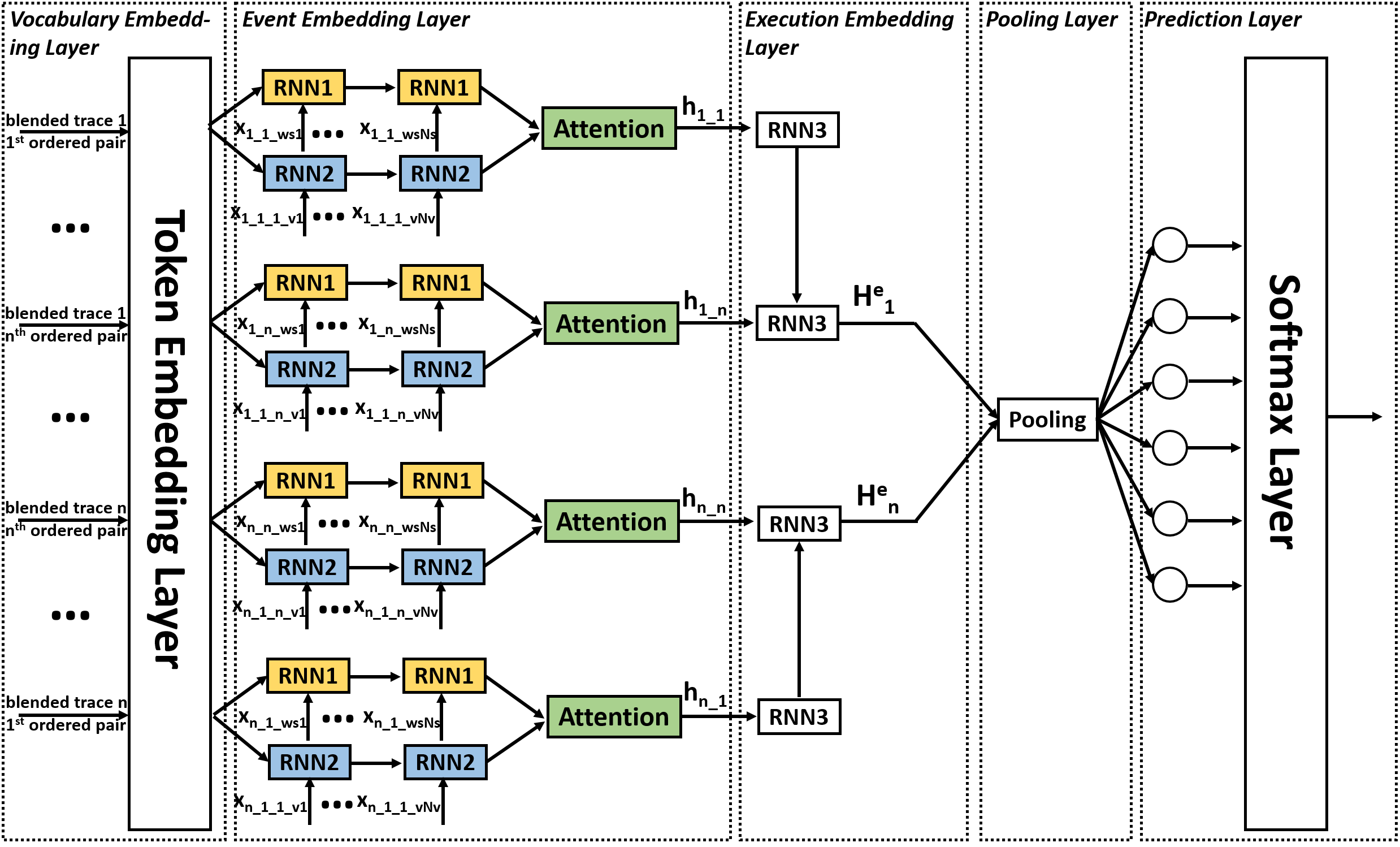
Figure 3. LiGer’s architecture.

4.1. LiGer’s Architecture

LiGer’s architecture is depicted in Figure 3. At a high level, LiGer uses three RNNs to encode an entire execution into a vector. To elevate the learning at the execution level to the program level, a pooling layer is designed to compress execution embeddings into program embeddings. Below, we split the entire network into five layers and discuss each layer in detail.

Terminology. Given a program $P$, we denote its set of tokens as $w_{P_{1}},\cdot\cdot\cdot,w_{P_{N_{p}}}$. Each token $w_{P_{i}}\in\mathcal{D}_{s}$ where $\mathcal{D}_{s}$ is the set of all tokens extracted from all programs in our dateset. Within $P$’s token set, $w_{v_{1}},\cdot\cdot\cdot,w_{v_{N_{v}}}$ denote the variables. To turn $P$ in its source code form to the format LiGer requires, we symbolically execute $P$ to obtain $U$ distinct paths, where each path $\sigma_{i}$ is associated with a condition $\phi_{i}$. By solving $\phi_{i}$, we obtain concrete traces $\epsilon_{i\_1},\cdot\cdot\cdot,\epsilon_{i\_N_{\epsilon}}$. We encode each statement in $\sigma_{i}$ as a sequence of tokens $[w_{s_{1}},\cdot\cdot\cdot,w_{s_{N_{s}}}]$, and each program state in a concrete trace, $\epsilon_{i\_i^{\prime}}$, as a tuple of values $(v_{1},\cdot\cdot\cdot,v_{N_{v}})$ where $v_{i}\in\mathcal{D}_{d}$ is the value of $w_{v_{i}}$. $\mathcal{D}_{d}$ refers to the set of all values any variable has ever been assigned in any concrete trace of any program in our dataset.

Vocabulary Embedding Layer. In this layer, each $w_{i}\in\mathcal{D}_{s}$ and $v_{i}\in\mathcal{D}_{d}$ will be assigned a vector. Consider the $j$-th statement in $\sigma_{i}$, after the vocabulary embedding phase, the statement will be encoded as $[x_{i\_j\_w_{s_{1}}},\cdot\cdot\cdot,x_{i\_j\_w_{s_{N_{s}}}}]$. Similarly, the state created by $\sigma_{i}$’s $j$-th statement in $\epsilon_{i\_i^{\prime}}$ will be encoded as $(x_{i\_i^{\prime}\_j\_v_{1}},\cdot\cdot\cdot,x_{i\_i^{\prime}\_j\_v_{N_{v}}})$.

Fusion Layer. This layer embeds each statement in $\sigma_{i}$ and each state in $\epsilon_{i\_i^{\prime}}$ before fusing the two feature dimensions, which forms the core of our blended approach. To facilitate the later presentation, we introduce and formalize the notion of blended traces.

Definition 4.0.

(Blended Trace) Given a symbolic trace $\sigma$ and multiple concrete traces, $\epsilon_{1},\cdot\cdot\cdot,\epsilon_{n}$ that traverse the same program path as $\sigma$, a blended trace, $\lambda$, is a sequence of the form $(\theta_{i}\rightarrow\theta_{i+1})^{*}$, where $\theta_{i}$ is an ordered pair <$e_{i},S_{i}$>, where $e_{i}$ is a statement in $\sigma$ and $S_{i}=\{s_{i\_1},\cdot\cdot\cdot,s_{i\_{N_{\epsilon}}}\}$ is the set of program states $e_{i}$ created in $\epsilon_{1},\cdot\cdot\cdot,\epsilon_{N_{\epsilon}}$.

For simplicity, we assume that a blended trace $\lambda_{i}$ is composed of $\sigma_{i}$ and two concrete traces, $\epsilon_{i\_1}$ and $\epsilon_{i\_2}$. Given the $j$-th ordered pair in $\lambda_{i}$, the first RNN computes the embedding of the statement $(x_{i\_j\_w_{s_{1}}},\cdot\cdot\cdot,x_{i\_j\_w_{s_{N_{s}}}})$ to be (based on an abstraction of the computation defined in Equation 1):

$$h_{i\_j\_w_{s_{N_{s}}}}=f_{1}(x_{i\_j\_w_{s_{N_{s}}}},h_{i\_j\_w_{s_{N_{s}-1}}})$$

The second RNN embeds the two program states in the $j$-th ordered pair as

$$h_{i\_1\_j\_v_{N_{v}}} =f_{2}(x_{i\_1\_j\_v_{N_{v}}},h_{i\_1\_j\_v_{N_{v}-1}})$$

$$h_{i\_2\_j\_v_{N_{v}}} =f_{2}(x_{i\_2\_j\_v_{N_{v}}},h_{i\_2\_j\_v_{N_{v}-1}})$$

Now we present the idea key to LiGer’s success. To combine the strengths of both approaches, we fuse the vector representations across the feature dimensions to compute a single embedding of each ordered pair in a blended trace. Specifically, we adopt the attention mechanism to allocate a weight for each feature vector. Assume $H^{e}_{i\_j-1}$ denotes the embedding that represents $\lambda_{i}$ before $j$-th ordered pair, we compute the attention weights of $h_{i\_j\_w_{s_{N_{s}}}}$, $h_{i\_1\_j\_v_{N_{v}}}$ and $h_{i\_2\_j\_v_{N_{v}}}$ below:

$$\alpha_{i\_j\_w_{s_{N_{s}}}} =\frac{\mathit{exp}(\mu_{i\_j\_w_{s_{N_{s}}}})}{\mathit{exp}(\mu_{i\_j\_w_{s_{N_{s}}}})+\mathit{exp}(\mu_{i\_1\_j\_v_{N_{v}}})+\mathit{exp}(\mu_{i\_2\_j\_v_{N_{v}}})}$$

$$\alpha_{i\_1\_j\_v_{N_{v}}} =\frac{\mathit{exp}(\mu_{i\_1\_j\_v_{N_{v}}})}{\mathit{exp}(\mu_{i\_j\_w_{s_{N_{s}}}})+\mathit{exp}(\mu_{i\_1\_j\_v_{N_{v}}})+\mathit{exp}(\mu_{i\_2\_j\_v_{N_{v}}})}$$

$$\alpha_{i\_2\_j\_v_{N_{v}}} =\frac{\mathit{exp}(\mu_{i\_2\_j\_v_{N_{v}}})}{\mathit{exp}(\mu_{i\_j\_w_{s_{N_{s}}}})+\mathit{exp}(\mu_{i\_1\_j\_v_{N_{v}}})+\mathit{exp}(\mu_{i\_2\_j\_v_{N_{v}}})}$$

where $\oplus$ denotes vector concatenation and $\mu_{i\_j\_w_{s_{N_{s}}}}$, $\mu_{i\_1\_j\_v_{N_{v}}}$ and $\mu_{i\_2\_j\_v_{N_{v}}}$ are defined as follows ($a_{1}$ stands for a feedforward neural network):

$$\mu_{i\_j\_w_{s_{N_{s}}}} =a_{1}(h_{i\_j\_w_{s_{N_{s}}}}\oplus H^{e}_{i\_j-1})$$

$$\mu_{i\_1\_j\_v_{N_{v}}} =a_{1}(h_{i\_1\_j\_v_{N_{v}}}\oplus H^{e}_{i\_j-1})$$

$$\mu_{i\_2\_j\_v_{N_{v}}} =a_{1}(h_{i\_2\_j\_v_{N_{v}}}\oplus H^{e}_{i\_j-1})$$

Using the attention weights, we compute the embedding of the $j$-th ordered pair in $\lambda_{i}$ as

$$h_{i\_j}=\alpha_{i\_j\_w_{s_{N_{s}}}}*h_{i\_j\_w_{s_{N_{s}}}}+\alpha_{i\_1\_j\_v_{N_{v}}}*h_{i\_1\_j\_v_{N_{v}}}+\alpha_{i\_2\_j\_v_{N_{v}}}*h_{i\_2\_j\_v_{N_{v}}}$$

Note that we evenly distribute the weights across all feature vectors embedded from the first ordered pair in any blended trace.

Executions Embedding Layer. Given $h_{i\_1},\cdot\cdot\cdot,h_{i\_|\lambda_{i}|}$, the embeddings for all ordered pairs in $\lambda_{i}$, we use the third RNN to model the flow of the blended trace.

$$H^{e}_{i}=f_{3}(H^{e}_{i\_|\lambda_{i}|-1},h_{i\_|\lambda_{i}|})$$

where $H^{e}_{i\_j}$ is the embedding that represents the partial blended trace from the first ordered pair to the $j$-th ordered pair (including the $j$-th ordered pair). In other words, $H^{e}_{i}$ represents the entire $\lambda_{i}$.

Programs Embedding Layer. We design a pooling layer to compress the embeddings of all the blended traces, $H^{e}_{1},\cdot\cdot\cdot,H^{e}_{U}$, one for each path to a program embedding $\mathcal{H}_{P}$.

$$\mathcal{H}_{P}=\mathit{max\_pooling}(H^{e}_{1},\cdot\cdot\cdot,H^{e}_{U})$$

Loss Function. The network is trained to minimize the cross-entropy loss on a softmax over the prediction labels. Training is performed using a gradient descent based algorithm which utilizes back-propagation to adjust the weight of each parameter.

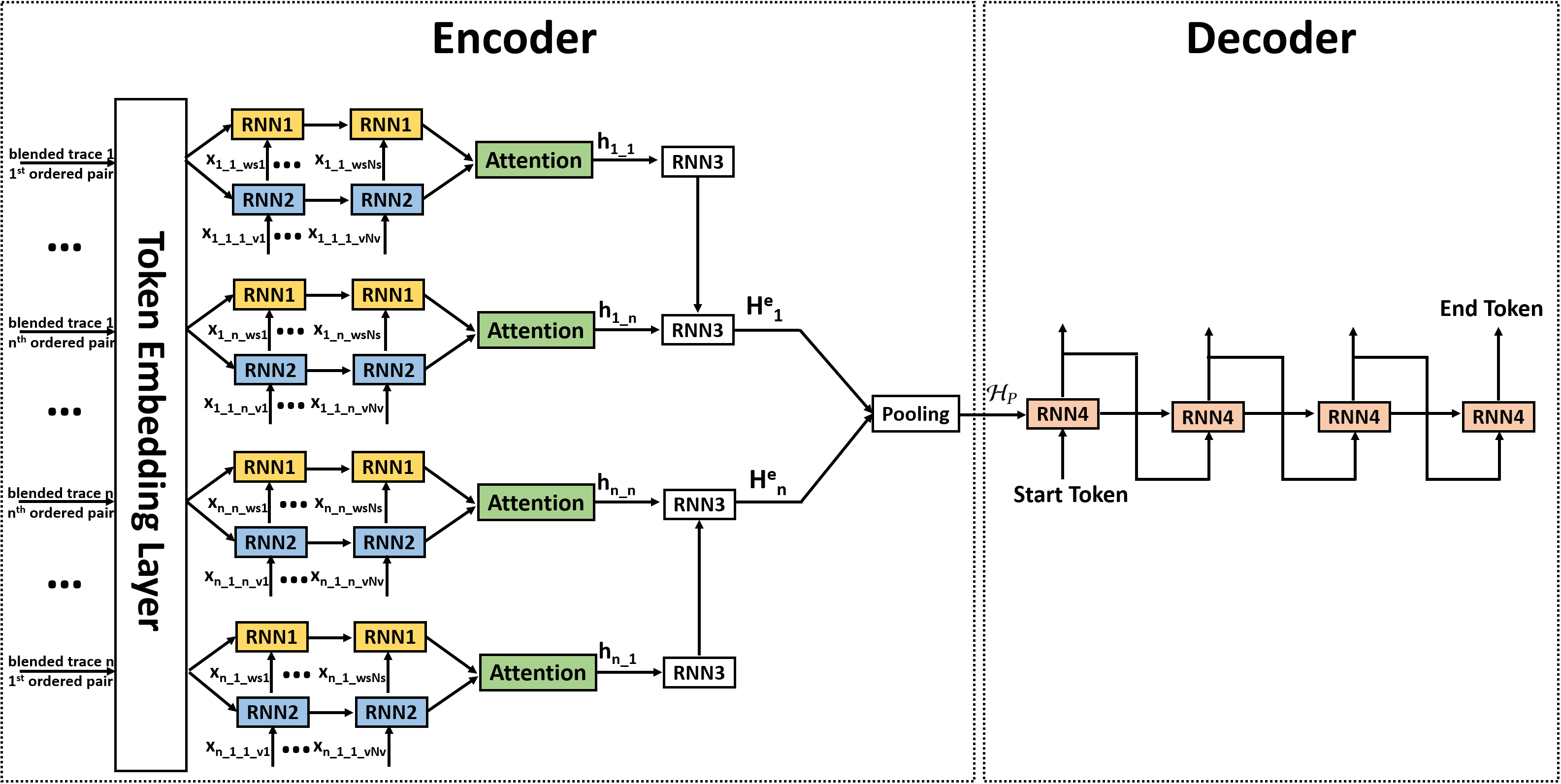
Figure 4. Extending LiGer into an encoder-decoder architecture.

4.2. Extension of LiGer

We also extend LiGer into an encoder-decoder architecture to solve the problem of method name prediction. Specifically, we remove the program embedding layer from LiGer and add a decoder to predict method names as sequences of words. Figure 4 depicts the extended architecture.

Encoder. We cut LiGer’s last layer to play the role of the encoder. Given a program $P$, the encoder outputs $\mathcal{H}_{P}$, and $\{\{H^{e}_{i\_j}|j\in[1,|\lambda_{i}|]\}|i\in[1,U]\}$, the set of embeddings for each blended trace of program $P$.

Decoder. We use another RNN to be the decoder. For initialization, we provide the decoder with the program embedding $\mathcal{H}_{P}$. The decoder also receives a special token to begin, and emits another to end the generation.

Attention. As explained in Section 3.2, we incorporate the attention mechanism to the extended architecture to aid the decoding process. Unlike the attention neural network introduced previously where the decoder attends over the input symbols from a single source sentence, our decoder attends over the flow of all blended traces (i.e. $\{\{H^{e}_{i\_j}|j\in[1,|\lambda_{i}|]\}|i\in[1,U]\}$).

We recompute the context vector $c_{t}$ (defined in Equation 2) for each generated word $y_{t}$ as:

$$c_{t}=\sum_{i=1}^{U}\sum_{j=1}^{|\lambda_{i}|}\alpha_{t\_i\_j}H^{e}_{i\_j}$$

Each attention weight $\alpha_{t\_i\_j}$ is computed by

$$\alpha_{t\_i\_j}=\frac{\mathit{exp}(\mu_{\mathit{t\_i\_j}})}{\sum_{i=1}^{U}\sum_{j=1}^{|\lambda_{i}|}\mathit{exp}(\mu_{t\_i\_j})}$$

where $\mu_{t\_i\_j}=a_{2}(H^{d}_{t-1},H^{e}_{i\_j})$ is the attention score which measures how well each $H^{e}_{i\_j}$ correlates with the previous hidden state of the decoder, $H^{d}_{t-1}$. The parameter $a_{2}$ stands for a feedforward neural network that is jointly trained with other components in the extended architecture. Figure 5 depicts a graphical illustration of the attention mechanism built into the extended architecture.

5. Implementation

In this section, we first describe how to parse programs into LiGer’s required format, and then present the implementation details of LiGer.

5.1. Data Pre-Processing

To obtain the data format LiGer requires, we weigh the option of running a symbolic execution engine to obtain symbolic traces. However, as LiGer does not particularly require executions to achieve high code coverage and the practical limitations of symbolic execution complicates our implementation, we choose to execute programs with random inputs to obtain the concrete traces, from which we derive the symbolic traces. As a final step, we construct the blended traces.

Since we mostly deal with C# and Python programs, we use the Microsoft Roslyn compiler framework and IronPython for those program pre-processing tasks, including extracting a program’s abstract syntax tree (AST) and instrumenting the program’s source code. As for program executions, we use Roslyn’s emit API and IronPython’s interpreter.

5.2. Implementation of LiGer

LiGer is implemented in Tensorflow. All RNNs have one single recurrent layer with 100 hidden units. We adopt random initialization for weight initialization. Our vocabulary has 7,188 unique tokens (i.e., tokens of all programs and the values of all variables at each time step), each of which is embedded into a 100-dimensional vector. All networks are trained using the Adam optimizer (Kingma and Ba, 2014) with the learning and the decay rates set to their default values (i.e., learning rate = 0.0001, beta1 = 0.9, beta2 = 0.999) and a mini-batch size of 100. We use five Red Hat Linux servers, each of which hosts four Tesla V100 GPUs (with 32GB GPU memory).

Figure 5. Graphic illustration of the attention mechanism in the extended architecture.

6. Evaluation

This section presents the details of our extensive and comprehensive evaluation. First, we evaluate LiGer on COSET. Then, we perform ablations to study and evaluate LiGer’s internal design and realization. Finally, we evaluate how well the extension of LiGer predicts method names.

6.1. Evaluation of LiGer on COSET

We briefly introduce COSET and then present in detail each of the conducted experiments.

6.1.1. Introduction of COSET

COSET is a recently proposed benchmark framework that aims at providing a consistent baseline for evaluating the performance of neural program embeddings.

COSET’s Dataset. COSET contains a dataset consisting of close to 85K programs developed by a large number of programmers while solving ten coding problems. Programs are handpicked to ensure sufficient variations (e.g., coding style, algorithmic choices or structure). The dataset was manually analyzed and labeled. The work was done by fourteen PhD students and exchange scholars at the University of California, Davis. To reduce the labeling error, most of the programs solving the same coding problem are assigned to a single participant. Later the results are cross-checked among all participants for validation. The whole process took more than three months to complete. Participants came from different research backgrounds such as programming language, database, security, graphics, machine learning, etc. All participants were interviewed and tested for their knowledge of program semantics. The labeling is on the basis of execution semantics (e.g., bubble sort, insertion sort, merge sort, etc., for a sorting routine). Certain variations are discounted to keep the total number of labels manageable. For example, local variables for temporary storage are ignored, so are iterative styles (looping or recursion) and the sorting order (descending or ascending). After obtaining COSET, we removed the problem of printing the chessboard whose execution does not require external inputs. Readers are invited to consult the supplemental materials for the descriptions of all coding problems and the list of all labels.

To collect execution traces, we run each program with a large number of randomly generated inputs. Our intention is to trigger a large fraction of the program paths, and cover each path with a sufficient amount of executions. We remove programs that fail to pass all test cases (i.e., crashes or having incorrect results) from the dataset. In the end, we are left with 65,596 programs which we split into a training set containing 45,596 programs, a validation set of 9,000 programs and a test set with the remaining 9,000 programs (Table 1).

Benchmarks Training Validation Testing Find Array Max Difference 5,821 1,000 1,000 Check Matching Parenthesis 3,451 1,000 1,000 Reverse a String 6,087 1,000 1,000 Sum of Two Numbers 6,635 1,000 1,000 Find Extra Character 5,056 1,000 1,000 Maximal Square 4,862 1,000 1,000 Maximal Product Subarray 5,217 1,000 1,000 Longest Palindrome 5,480 1,000 1,000 Trapping Rain Water 2,987 1,000 1,000 Total 45,596 9,000 9,000

Table 1. Dataset used in semantic classification.

COSET’s Task. The prediction task that COSET provides is semantic classification. That is a model is required to predict the category where a program falls based on its semantics. In other words, not only does the model need to classify which coding problem that a program solves, but also which strategy that the program adopts in its solution. We use prediction accuracy and F1 score as the evaluation metrics.

COSET’s Transformations. COSET also includes a suite of program transformations. These transformations when applied to the base dataset can simulate natural changes to program code due to optimization and refactoring. Wang et al. use those transformations in COSET for two purposes. First, they are used to measure the stability of model predictions. By applying only semantically-preserving transformations, one can test how frequently a model changes its original predictions. The more frequently a prediction changes, the less precise the model is. Second, when a model makes an incorrect classification, the transformations are used to identify the root cause of a misclassification for debugging. In this paper, we measure the stability of each model by applying semantically-preserving transformations on the COSET’s dataset.

6.1.2. Evaluating LiGer’s performance

This experiment compares LiGer with several other DNNs targeting learning program representations.

• GGNN: GGNN is first proposed by Li et al. (2015) and later utilized by Allamanis et al. (2017) to predict variable misuse bugs in a program. The idea is to construct a graph out of a program’s AST along with additional semantic edges that are manually designed to improve a graph’s expressiveness. Those edges denote variable read/write relations, orders of leaf nodes in the AST, guarding conditions of statements, etc. In this experiment, we strip off the prediction layer and average all nodes in a graph to be the program embedding.

• code2vec: code2vec is proposed by Alon et al. (2019) to predict method names based on a large, cross-project corpus. The approach first decomposes the code for a program to a collection of paths in its abstract syntax tree, and then learns to represent each path as well as aggregating a set of them. We use code vector --- the aggregation of context vectors --- to represent a program.

• DYPRO: We also use DYPRO (Wang, 2019), another DNN that learns program representations from program executions. To allow a meaningful direct comparison, we feed LiGer and DYPRO the same collection of execution traces and observe differences in their performance.

As depicted in Figure 5(a), LiGer is the most accurate model among all, albeit not a substantial improvement over DYPRO. In contrast, static models (both GGNN and code2vec) perform significantly worse. In terms of the F1 score, LiGer also achieves the best results and significantly outperforms GGNN and code2vec (Figure 5(b)).

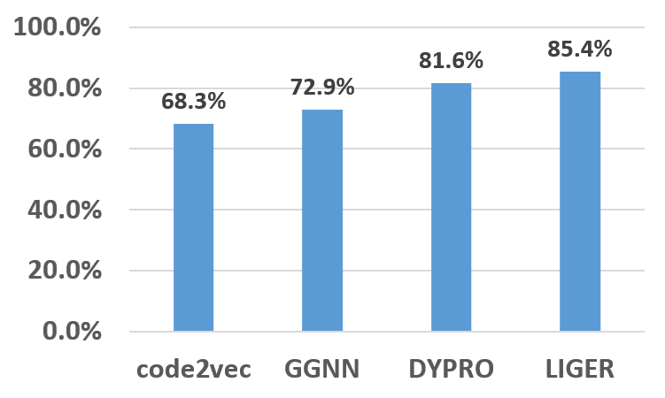
(a) The comparison of models using accuracy.

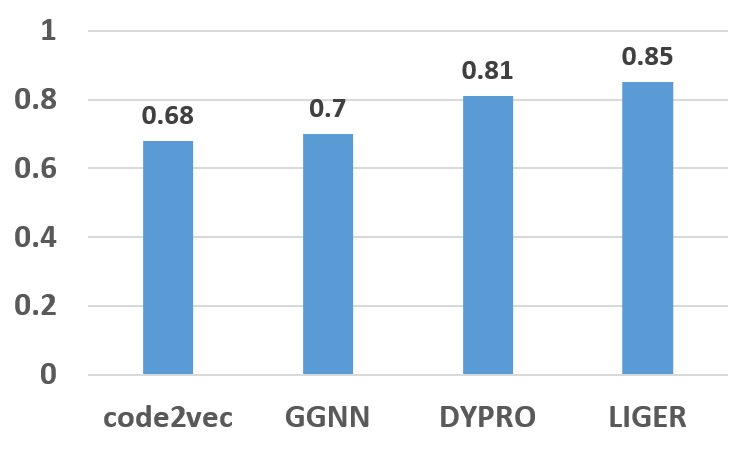
(b) The comparison of models using F1 score.

Figure 6. Comparing all models with the semantic classification task.

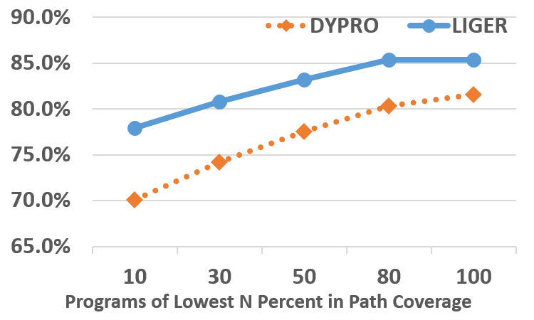
(a) Comparison on prediction accuracy.

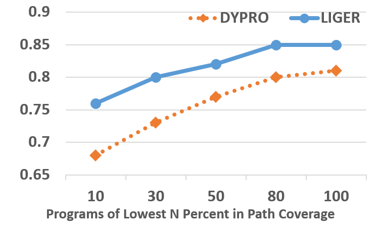
(b) Comparison on F1 score.

Figure 7. Comparison of LiGer against DYPRO for programs with increasing path coverage.

We performed another experiment for a more in-depth understanding of the comparison between LiGer and DYPRO. In particular, we split COSET’s testing programs into subgroups according to their path coverage (i.e., lowest 10% of programs to 100% in terms of path coverage) and evaluate how the models compare on each subgroup. We reuse both models from the previous experiment without retraining. As depicted in Figures 6(a) and 6(b), when tested on the lowest 30% of programs ranked by path coverage, LiGer outperforms DYPRO by a wide margin. The gap shrinks on programs with higher coverage, indicating similar performances of the two models on these programs. The results indicate that, although LiGer does not significantly improve DYPRO in overall accuracy, it is more reliable to generalize to unseen programs, particularly those on which high path coverage is difficult to obtain. Subsequent experiments are designed to understand the reasons behind this observation.

6.1.3. Reliance on Program Executions

We examine to what degree LiGer relies on executions to produce precise program embeddings. Reusing the semantic classification task, we evaluate LiGer from two aspects. First, we randomly reduce the number of concrete traces used to construct a blended trace while keeping the total number of symbolic traces constant for each program in both COSET’s training and testing sets. In other words, we aim to find out how LiGer would perform when each symbolic trace is accompanied with a fewer number of concrete traces.

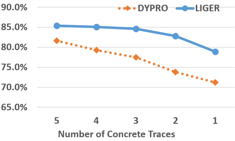
(a) Change of accuracy for LiGer when number of executions per path is randomly reduced.

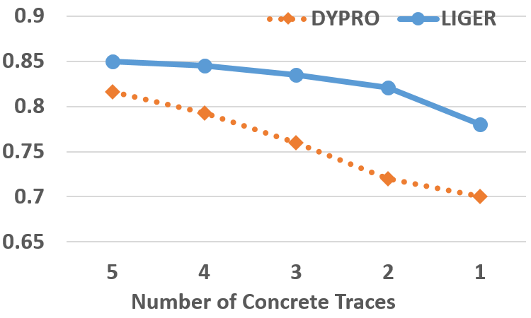
(b) Change of F1 score for LiGer when the number of executions per path is randomly reduced.

Figure 8. LiGer’s results when the number of executions per path is randomly reduced.

Figures 7(a) and 7(b) show results for this experiment. In general, reducing concrete traces in a blended trace path has a small effect on LiGer’s performance. Perhaps more unexpectedly, LiGer exhibits almost the same accuracy and F1 score when it is supplied with no less than three concrete traces. To dig deeper, we also investigate how attention weights of each symbolic trace change when executions are down-sampled. We observe that, upon model convergence, the attention weight for each statement along each symbolic trace is 5.98 on average, and the weight stays largely unchanged throughout the reduction. Furthermore, the rest of the attention weight (i.e., 4.12) is almost evenly split into the concrete traces regardless their number. This finding shows that LiGer relies more on the static (symbolic) feature dimension while generalizing from the training programs. Meanwhile, it views concrete traces as parallel instantiations of the same symbolic trace. Most importantly, LiGer is capable of compensating the loss of concrete traces by increasing the importance of the remaining ones, therefore keeping its accuracy constant. Specifically, when left with two concrete traces in a blended trace, LiGer can still achieve more than a 83% (resp. 0.82) accuracy (resp. F1 score). In contrast, DYPRO suffers a significant performance drop, empirically confirming its far higher demand for concrete traces.

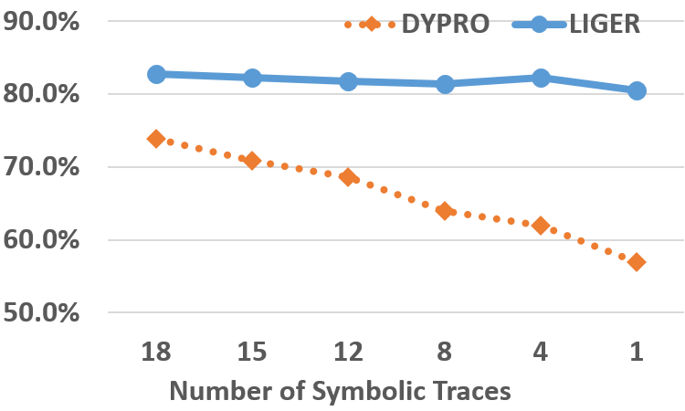
(a) Change of accuracy for DYPRO and LiGer when program paths are reduced but branch coverage is preserved for each program.

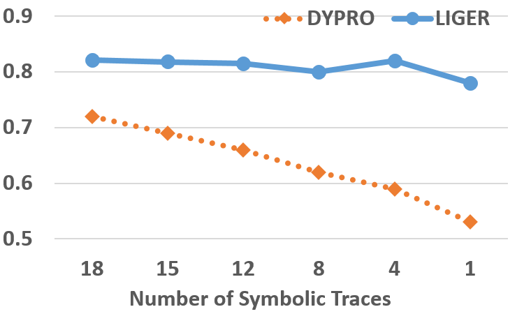
(b) Change of F1 score for DYPRO and LiGer when program paths are reduced but branch coverage is preserved for each program.

Figure 9. Accuracy trend for LiGer and DYPRO when branch coverage is preserved for each program throughout path reduction.

Next, we investigate how LiGer reacts when the number of symbolic traces decreases. We have identified a minimum set of symbolic traces for each program in COSET’s dataset that achieve the same branch coverage as before. We remove symbolic traces that are not in the minimum set and examine how path coverage affects LiGer’s accuracy. In this experiment, we randomly select two out of the original five concrete traces, from which we generate a minimum set of blended traces. As a baseline, we show how LiGer compares against DYPRO on the same concrete traces throughout path reduction.

When branch coverage is preserved during path reduction, LiGer’s performance is largely unaffected (Figure 9), indicating its strong resilience to reduced program paths. Even if training and testing on the minimum set of blended traces, LiGer is more accurate than DYPRO trained and tested on the entire set of concrete traces (82.3% vs. 81.6% in accuracy, and 0.82 vs. 0.81 in F1 score). As the average size of the minimum set of symbolic traces is calculated to be 4.7 (i.e., 9.4 concrete executions) for each program, LiGer used nearly 10x fewer executions covering almost 74% fewer program paths. By learning from the minimum set of blended traces, LiGer also reduces the training time from 273 hours to 38 hours under the same setup.

Our findings indicate that LiGer depends far less on program executions than DYPRO. In addition, the results also explain the superior performance LiGer exhibits on the COSET’s testing programs that are difficult to cover (Figure 7). Because LiGer does not require very high code coverage in order to produce precise program embeddings, it lessens its reliance on both the number and diversity of program executions.

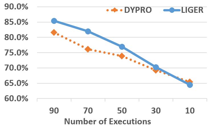
(a) Change of accuracy for DYPRO and LiGer when executions are randomly reduced.

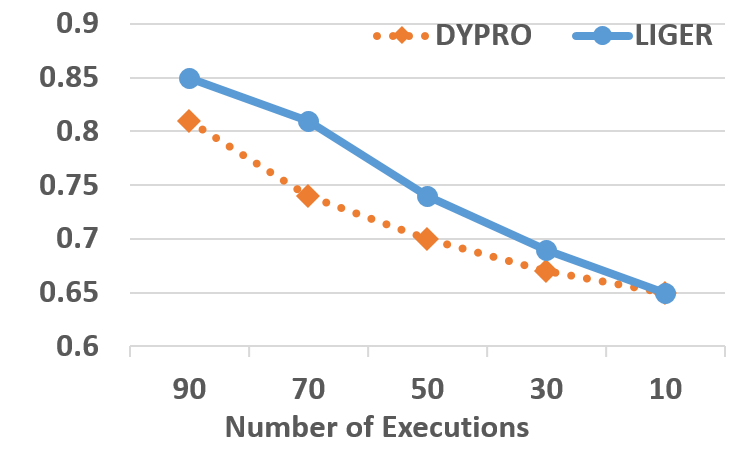
(b) Change of F1 score for DYPRO and LiGer when executions are randomly reduced.

Figure 10. Accuracy trend for LiGer and DYPRO when randomly down-sampling executions.

To verify the validity of these two experiments, we conduct another study in which we randomly reduce both symbolic and concrete traces, and construct blended traces accordingly. Results (Figure 10) show that LiGer overall still performs slightly better than DYPRO. However, it is not nearly as tolerant of data loss as the two above experiments have shown. Thus, to conclude, compared to DYPRO, LiGer displays much less reliance on program executions. Specifically, we show that neither the reduction of blended traces nor the decrease in path coverage significantly affects LiGer’s performance.

6.1.4. Comparison on Model Stability

In this experiment, we measure the stability for each model prediction by applying the semantically-preserving program transformations to COSET’s test set. Those transformations are routinely performed by compilers for code optimization (e.g., constant and variable propagation, dead code elimination, loop unrolling and hoisting). Specifically, we apply the transformations to each test program in Table 1 to create a new test set. Programs with no applicable transformations are excluded from the new test set. We then examine if the models make the same prior predictions in the semantic classification task.

Table 2 presents the results. The number in each cell denotes the percentage of programs in the new test set on which a model has changed its prediction. Overall, LiGer is the most stable model against those program transformations, and is significantly more stable than both static models.

Model Constant and Variable Propagation Dead Code Elimination Loop Unrolling Hoisting code2vec 8.6% 12.4% 23.9% 12.2% GGNN 6.8% 7.4% 16.8% 10.9% DYPRO 3.4% 4.1% 6.8% 1.8% LiGer 3.4% 3.5% 7.9% 1.3%

Table 2. Results on measuring model stability, measured as percentage of changed predictions when applying semantics-preserving transformations.

(a) Change of accuracy before and after removing the static feature dimension from LiGer.

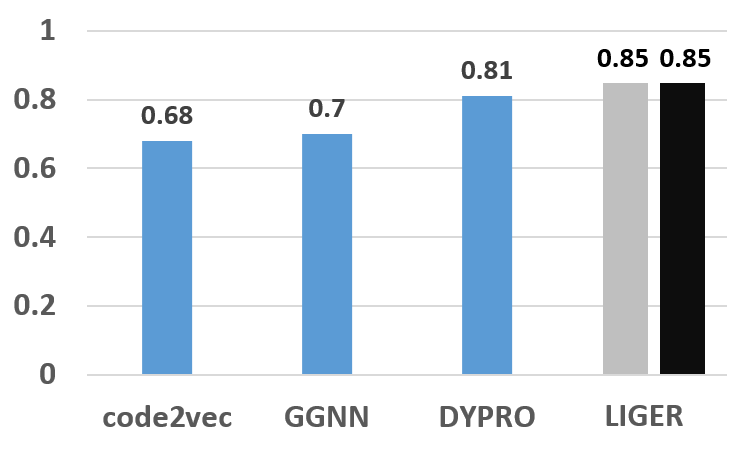
(b) Change of F1 score before and after removing the static feature dimension from LiGer.

Figure 11. Effects of the static feature dimension in LiGer for the semantic classification task. Light bars denote results before, while dark bars denote results after the ablation.

6.2. Ablation Study

In this section, we conduct an ablation study to understand the contribution of each component in LiGer’s architecture. Since all layers except the fusion layer are essential to LiGer’s functionality, our ablation study will only examine the causality among components in the fusion layer, more precisely, the effect of both feature dimensions as well as the attention mechanism that fuses the feature dimensions. To evaluate each new configuration of LiGer, we use model accuracy and data reliance as the two metrics in the semantics classification task.

6.2.1. Removing Static Feature Dimension

First, we remove the symbolic trace from the feature representation. As a result, RNN1 is no longer needed and removed from LiGer’s architecture. Note that the resulting configuration is not identical to DYPRO’s architecture where an embedding for each execution is learned separately. In contrast, LiGer learns an embedding for a multitude of executions along the same program path. We use the same concrete traces for each program in COSET to repeat the experiment on semantics classification.

As depicted in Figure 11, after removing the static feature dimension, LiGer exhibits the same prediction accuracy (hereinafter light/dark shapes denote LiGer’s results before/after the ablation) and F1 score. This indicates that, when given abundant concrete traces to learn, LiGer is able to generalize from the dynamic features alone, therefore, symbolic traces becomes expendable. In addition, even without the static feature dimension, LiGer still significant outperforms both static models in accuracy and F1 score as shown in Figures 10(a) and 10(b).

Next, we aim to understand how dependent LiGer becomes on executions after removing the static feature dimension. In our ablation study, we always maintain the branch coverage of a program while decreasing both the numbers of symbolic and concrete traces. For brevity, we combine the results of reducing symbolic and concrete traces in the same diagram. As shown in Figures 12, after removing the static feature dimension, LiGer displays a similar performance trend to DYPRO. In other words, LiGer becomes more dependent on program executions, manifested in the significantly poorer results while learning from few concrete traces. This finding reveals that it is the static feature dimension that contributes to the moderate reliance LiGer has on program executions.

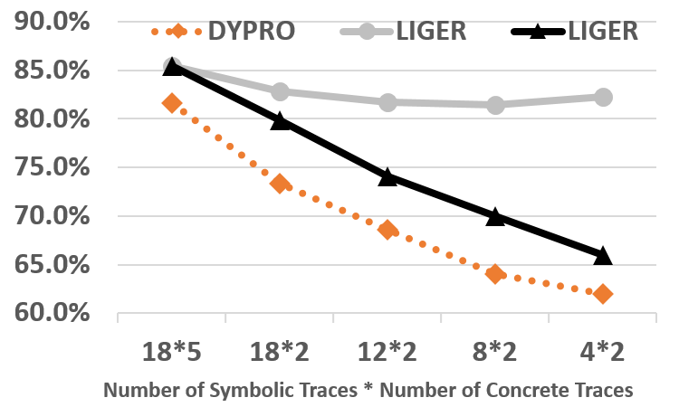
(a) Comparing LiGer’s accuracy trend before and after removing static features when both symbolic and concrete traces are reduced.

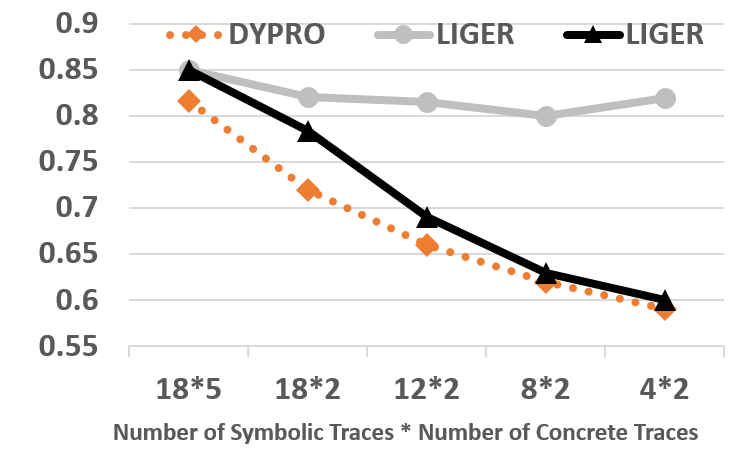
(b) Comparing LiGer’s F1 score trend before and after removing static features when both symbolic and concrete traces are reduced.

Figure 12. The effect of static feature dimension on models’ reliance on executions.

(a) Change of accuracy before and after removing the dynamic feature dimension from LiGer.

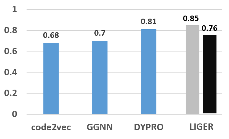
(b) Change of F1 score before and after removing the dynamic feature dimension from LiGer.

Figure 13. The effect of the dynamic feature dimension in LiGer for the semantics classification task.

6.2.2. Removing Dynamic Feature Dimension

We remove the dynamic feature dimension from LiGer to reveal its contribution to the entire network. Since LiGer is left with the symbolic traces only, each statement in the trace will receive the full attention weight in the fusion layer. Like the prior experiment, we first measure LiGer’s accuracy for the semantics classification task.

As depicted in Figures 12(a) and Figure 12(b), removing dynamic feature has a larger impact on LiGer’s precision. In particular, both accuracy and F1 score drop notably despite still being more accurate than both the static models by a reasonable margin. This finding confirms the challenges of learning precise program embeddings from symbolic program features directly. Even though symbolic traces reflect certain level of the runtime information, LiGer does not manage to learn precise program embeddings. Next, we study LiGer’s reliance blended traces.

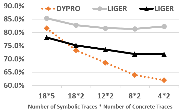
(a) Comparing LiGer’s accuracy trend before and after removing the dynamic features both symbolic and concrete traces are reduced.

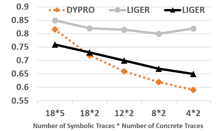
(b) Comparing LiGer’s F1 score trend before and after removing the dynamic features both symbolic and concrete traces are reduced.

Figure 14. The effect of the dynamic feature dimension in LiGer on the model reliance on executions.

After removing the dynamic feature dimension, LiGer is still shown quite robust against trace reduction. Even though LiGer starts at a lower accuracy and F1 score, it outperforms DYPRO as both the numbers of symbolic and concrete traces decrease (Figures 13(a) and 13(b)). In general, the accuracy trend LiGer displays correlates well before and after the removal of dynamic features. Thanks to the static feature dimension, LiGer does not suffer a significant accuracy drop.

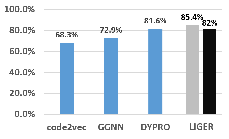
(a) Change of accuracy before and after removing the attention mechanism from fusion layer.

(b) Change of F1 score before and after removing the attention mechanism from fusion layer.

Figure 15. The effect of attention in the fusion layer for the semantics classification task.

6.2.3. Removing Attention

Finally, we remove the attention mechanism that controls the fusion of the two feature dimensions. To keep other components intact in the fusion layer, we evenly distribute the weights across all traces (i.e., symbolic and concrete) in a blended trace.

Figure 15 presents the results. Removing attention has a notable impact on LiGer. Although both accuracy and F1 score decrease, the drop is insignificant. This is an unexpected result. As concrete traces are still abundant, an increase in their attention weights should at least leads to a similar performance. Our hypothesis is that allocating constant weights disrupts the balance LiGer strikes for the two feature dimensions. Although the weights for the dynamic feature increase, the presence of static features limits LiGer’s ability to generalize. In terms of its reliance on program executions, LiGer becomes less accurate overall (Figure 16). The explanation is that, without the attention mechanism, symbolic program features will be allocated with lower weights. Therefore, the static feature dimension is unable to issue as strong signals as before to help LiGer learn, thus causing the drop in LiGer’s accuracy.

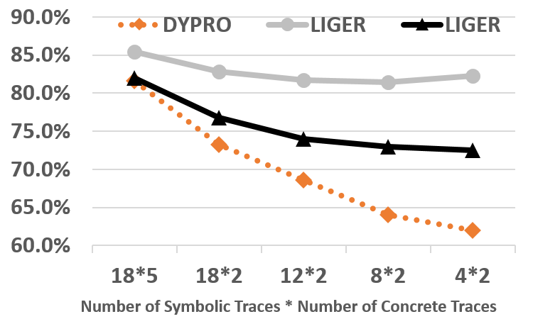
(a) Comparing LiGer’s accuracy trend before and after removing the attention mechanism in the fusion layer when both symbolic and concrete traces are reduced.

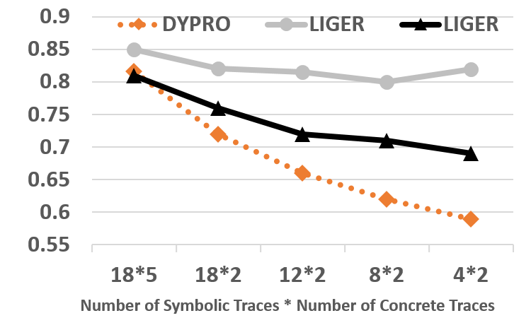
(b) Comparing LiGer’s F1 score trend before and after removing the attention mechanism in the fusion layer when both symbolic and concrete traces are reduced.

Figure 16. The effect of attention in the fusion layer on the model reliance on executions.

6.2.4. Summary

Finally, we summarize the role of each component in the fusion layer. To provide a direct comparison, we show the results of each new configuration of LiGer on the same diagram (Figure 17).

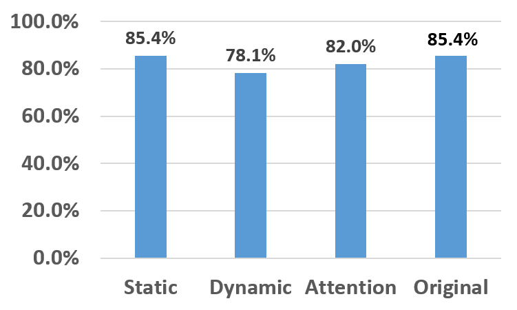
(a) Comparing LiGer’s accuracy in the semantics classification task for each ablation configuration.

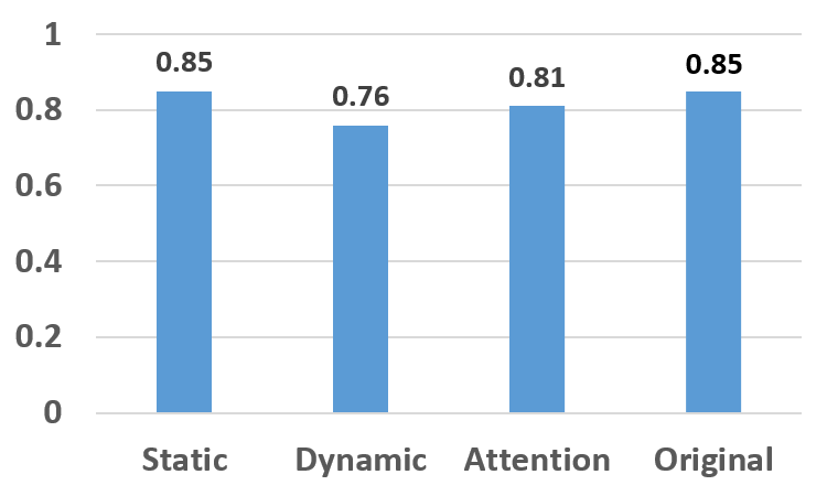
(b) Comparing LiGer’s F1 score in the semantics classification task for each ablation configuration.

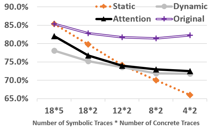
(c) Comparing LiGer’s accuracy trend for each ablation configuration when both symbolic and concrete traces are reduced but branch coverage is preserved.

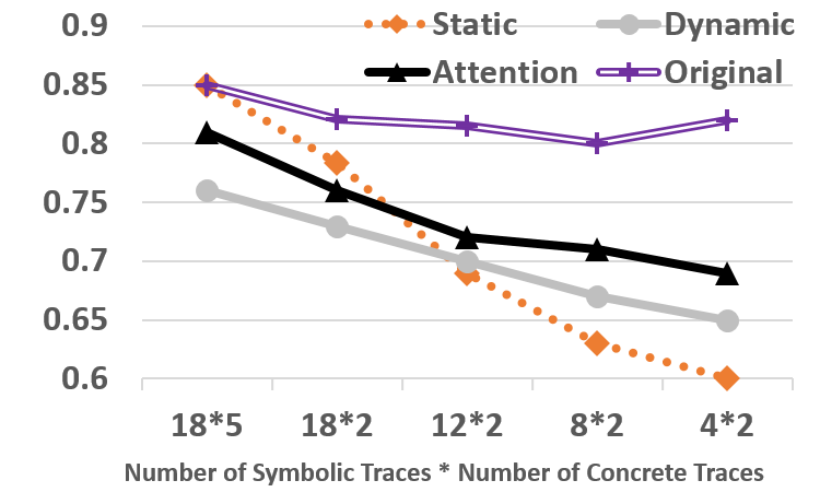
(d) Comparing LiGer’s F1 score trend for each ablation configuration when both symbolic and concrete traces are reduced but branch coverage is preserved.

Figure 17. Comparing different ablation configurations for LiGer.

To summarize, LiGer is the most precise model because of its generalization from the concrete traces specially in large quantities. However, the quality of training data is not always guaranteed, thus programs that are difficult to cover can affect LiGer’s performance. Even when code coverage is not an issue, using an excessive amount of concrete traces leads to prolonged and inefficient training. As a solution, combining symbolic and concrete traces significantly reduces the reliance that LiGer has on executions in both training and testing. In addition, this feature fusion is shown helpful in lowering LiGer’s need on traces with high path coverage, provided that the original branch coverage is still maintained for the targeted programs. An integral part of feature fusion is the attention mechanism which allocates greater weights to the static feature dimension than the dynamic one. In addition, the average weight of the static feature dimension remains largely constant when the number of concrete traces varies. Overall, we conclude that static program features play a more important role in feature fusion, even if they alone are not sufficient for training a precise model to represent program semantics.

6.3. Method Name Prediction

In this experiment, we examine if LiGer can accurately predict the name of a method, a problem studied in (Alon et al., 2019). Solving this task is a strong indication of LiGer’s capability in learning precise representations of program semantics.

Dataset. We have extracted over 300K functions from a company’s database that records candidates’ programs during coding interviews. The questions asked in the coding interviews are mostly algorithmic problems designed to evaluate a candidate’s coding skills (e.g., swapping two variables without extra memory, balancing a binary search tree and rotating a linked list). The function names given by the interviewers provide good descriptors for the functions’ behavior. Compared to the benchmark suite proposed in (Alon et al., 2019) which consists of simpler functions (e.g., contains, get and indexOf), our dataset is more challenging for a model to learn. All functions are written in either C# and Python. Similar to the prior experiments, we randomly execute each program to collect the concrete traces. By grouping concrete traces that traverse the same program path, we derive the set of symbolic traces. We construct fifteen blended traces, each of which is built upon five concrete traces. Similarly, we also prepare a minimum set of blended traces that maintain the same branch coverage as the entire set for each program in the dataset. The minimum set contains no greater than six traces. Each blended trace is composed of two concrete traces. Functions that do not pass all the test cases are removed from the dataset. In the end, we keep 174,922 functions in total which we split into a training set of 104,922, a validation and testing set of 35K each for this experiment.

Evaluation Metric. We have adopted the metric used by prior work (Alon et al., 2019) to measure precision, recall and F1 score over case insensitive sub-tokens. The rationale is that the prediction of a whole method name highly depends on that of the sub-words. For example, given a method named computeDiff, a prediction of diffCompute is considered a perfect answer (i.e., the order of the sub-words does not matter), a prediction of compute has a full precision, but low recall, and a prediction of computeFileDiff has full recall, but low precision.

Baselines. We compare LiGer and code2seq on solving the exact same tasks. code2seq is the state-of-the-art DNN in predicting function names. It also has a encoder-decoder architecture. The encoder represents a function as a set of AST paths, and the decoder uses attentions to select relevant paths while decoding.

We also include Transformer (Vaswani et al., 2017), arguably the state-of-the-art deep learning model for Neural Machine Translation (NMT).

Model Precision Recall F1 Score code2seq 0.49 0.33 0.39 Transformer 0.46 0.28 0.35 LiGer 0.64 0.52 0.57 LiGer (Minimum Set) 0.61 0.44 0.51

Table 3. Results on the models in predicting method names.

Results. We depict the results for each model in Table 3. When trained on the full set of executions, LiGer significantly outperforms both competing models in all three categories: precision, recall and F1 score. Even on the minimum set, LiGer still achieves better results than code2seq and Transformer. Compared to Transformer, code2seq displays a slightly better performance. We also present the F1 score for each model as the size of test functions increases. LiGer trained on the minimum set of blended traces again outperforms all the other baselines across all program lengths.

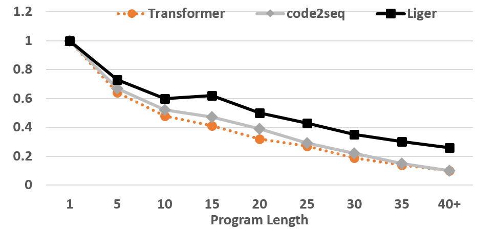
Figure 18. Comparing models performance as the size of function increases.

Examples. We pick two examples that LiGer gives perfect predictions, but neither code2seq nor Transformer does. The functions are shown in Figure 19.

For the function in Figure 18(a), code2seq predicts its name to be swapMatrix, while Transformer produces sortArray. Although the function does exhibit the behavior of swapping elements in a matrix, what it really does is rotating an image 90 degrees clockwise. LiGer is the only network that captures the high-level view of the function’s behavior. For the other function, all networks successfully generate the sub-words FibonacciSequence, however neither code2seq nor transformer captures Longest nor Length indicating the approaches’ lack of precision for learning program embeddings. We have also interacted with the code2seq tool at https://code2seq.com/ using the two functions in Figure 19 as inputs, and found that the model produces incorrect results.

⬇

public int rotateImage(List<List<int>> matrix)

{

if (matrix.Count == 0)

return -1;

int n = matrix.Count;

for (int i = 0; i < n; i++) {

for (int j = 0; j < i; j++) {

int temp = matrix[i][j];

matrix[i][j] = matrix[j][i];

matrix[j][i] = temp;

} }

for (int i = 0, j = n - 1; i < j; i++, j--) {

for (int k = 0; k < n; k++) {

int temp = matrix[k][i];

matrix[k][i] = matrix[k][j];

matrix[k][j] = temp;

} }

return 1;

}

(a) A function that rotates an image by 90 degrees (clockwise).

⬇

public int LongestFibonacciSequenceLength(List<int> sequence)

{

int length = sequence.Count;

int longest = 0;

for (int i = 0; i < sequence.Count - 1; i++) {

for (int j = i + 1; i < sequence.Count; j++) {

int first = sequence[i];

int second = sequence[j];

int count = 2;

while (sequence.Contains(first + second)) {

first = second;

second = first + second;

count++;

longest = Math.Max(longest, count);

} } }

return (longest > 2 ? longest : 0);

}

(b) A function that computes the length of the longest Fibonacci sequence.

Figure 19. Two example methods for which LiGer correctly predicts their names.

7. Related Work

In this section, we survey related work from three aspects: neural program embeddings, attention and word embeddings.

Neural Program Embeddings. Recently, learning neural program representations has generated significant interest in the program languages community. The goal is to learn precise and efficient representations to enable the application of DNNs for solving a range of program analysis tasks. As a first step, early methods (Gupta et al., 2017; Pu et al., 2016; Mou et al., 2016) primarily focus on learning syntactic features. Despite these pioneering efforts, these approaches do not precisely represent program semantics. More recently, a number of new deep neural architectures have been developed to tackle this issue (Allamanis et al., 2017; Wang et al., 2017; Wang, 2019; Alon et al., 2019). This line of work can be divided into two categories: dynamic and static. The former (Wang et al., 2017; Wang, 2019) learns from concrete program executions, while the latter (Allamanis et al., 2017; Alon et al., 2019) attempts to dissect program semantics from source code. Unlike these prior efforts, this paper presents an effective blended approach of learning program embeddings from both concrete and symbolic traces.

Attention. Attention has achieved ground-breaking results in many NLP tasks, such as neural machine translation (Bahdanau et al., 2014; Vaswani et al., 2017), computer vision (Ba et al., 2014; Mnih et al., 2014), image captioning (Xu et al., 2015) and speech recognition (Bahdanau et al., 2016; Chorowski et al., 2015). Attention models work by selectively choosing parts of the input to focus on while producing the output. code2vec is among the most notable that incorporate attention in their neural network architectures. Specifically, they attend over multiple AST paths and assign different weights for each before aggregating them into a program embedding. This paper uses attention to coordinate the combination of the two feature dimensions as well as to decode the method name as a sequence of words.

Word Embeddings. The seminal work (Mikolov et al., 2013b; Mikolov et al., 2013a) of Mikolov et al. on word2vec stimulated the field of learning continuous representation. They propose to embed words into a numerical space where those of similar meanings would appear in close proximity. By embedding words into vectors, they also discover that simple arithmetic operations can reflect the analogies among words (e.g. $\mathit{US}-\mathit{Washington}=\mathit{China}-\mathit{Beijing}$). word2ve, along with later efforts on learning representations of sentences and documents (Le and Mikolov, 2014), have greatly contributed to state-of-the-art results in many downstream tasks (Glorot et al., 2011; Bengio et al., 2003).

8. Conclusion

This paper has introduced a novel, blended approach of learning program embeddings from the combination of symbolic and concrete execution traces. Through an extensive evaluation, we have shown that our approach is not only the most accurate in classifying program semantics, but also significantly outperforms code2seq, the state-of-the-art in predicting method names. Our results have also shown that concrete executions when supplied in large quantities achieving good code coverage help train highly precise models. Symbolic traces, on the other hand, reduce dynamic models’ heavy reliance on executions. For its strong distinct benefits, we believe that our blended approach can be adapted to tackle a wide range of problems in program analysis and developer productivity.

References

- (1)
- Allamanis et al. (2017) Miltiadis Allamanis, Marc Brockschmidt, and Mahmoud Khademi. 2017. Learning to represent programs with graphs. arXiv preprint arXiv:1711.00740 (2017).
- Alon et al. (2018) Uri Alon, Omer Levy, and Eran Yahav. 2018. code2seq: Generating sequences from structured representations of code. arXiv preprint arXiv:1808.01400 (2018).
- Alon et al. (2019) Uri Alon, Meital Zilberstein, Omer Levy, and Eran Yahav. 2019. Code2Vec: Learning Distributed Representations of Code. Proc. ACM Program. Lang. 3, POPL, Article 40 (Jan. 2019), 29 pages.
- Ba et al. (2014) Jimmy Ba, Volodymyr Mnih, and Koray Kavukcuoglu. 2014. Multiple object recognition with visual attention. arXiv preprint arXiv:1412.7755 (2014).
- Bahdanau et al. (2014) Dzmitry Bahdanau, Kyunghyun Cho, and Yoshua Bengio. 2014. Neural machine translation by jointly learning to align and translate. arXiv preprint arXiv:1409.0473 (2014).
- Bahdanau et al. (2016) Dzmitry Bahdanau, Jan Chorowski, Dmitriy Serdyuk, Philemon Brakel, and Yoshua Bengio. 2016. End-to-end attention-based large vocabulary speech recognition. In International Conference on Acoustics, Speech and Signal Processing (ICASSP). 4945--4949.
- Bengio et al. (2003) Yoshua Bengio, Réjean Ducharme, Pascal Vincent, and Christian Janvin. 2003. A Neural Probabilistic Language Model. J. Mach. Learn. Res. 3 (March 2003), 1137--1155. http://dl.acm.org/citation.cfm?id=944919.944966
- Cho et al. (2014) Kyunghyun Cho, Bart Van Merriënboer, Caglar Gulcehre, Dzmitry Bahdanau, Fethi Bougares, Holger Schwenk, and Yoshua Bengio. 2014. Learning phrase representations using RNN encoder-decoder for statistical machine translation. arXiv preprint arXiv:1406.1078 (2014).
- Chorowski et al. (2015) Jan K Chorowski, Dzmitry Bahdanau, Dmitriy Serdyuk, Kyunghyun Cho, and Yoshua Bengio. 2015. Attention-based models for speech recognition. In Advances in neural information processing systems. 577--585.
- Devlin et al. (2014) Jacob Devlin, Rabih Zbib, Zhongqiang Huang, Thomas Lamar, Richard Schwartz, and John Makhoul. 2014. Fast and robust neural network joint models for statistical machine translation. In Proceedings of the 52nd Annual Meeting of the Association for Computational Linguistics (Volume 1: Long Papers). 1370--1380.
- Glorot et al. (2011) Xavier Glorot, Antoine Bordes, and Yoshua Bengio. 2011. Domain Adaptation for Large-scale Sentiment Classification: A Deep Learning Approach. In International Conference on International Conference on Machine Learning (ICML). 513--520.
- Gupta et al. (2017) Rahul Gupta, Soham Pal, Aditya Kanade, and Shirish Shevade. 2017. DeepFix: Fixing Common C Language Errors by Deep Learning.
- Henkel et al. (2018) Jordan Henkel, Shuvendu K. Lahiri, Ben Liblit, and Thomas Reps. 2018. Code Vectors: Understanding Programs Through Embedded Abstracted Symbolic Traces. In Proceedings of the 26th ACM Joint Meeting on European Software Engineering Conference and Symposium on the Foundations of Software Engineering (ESEC/FSE). 163--174.
- Kingma and Ba (2014) Diederik P Kingma and Jimmy Ba. 2014. Adam: A method for stochastic optimization. arXiv preprint arXiv:1412.6980 (2014).
- Le and Mikolov (2014) Quoc Le and Tomas Mikolov. 2014. Distributed Representations of Sentences and Documents. In International Conference on Machine Learning. 1188--1196.
- Li et al. (2015) Yujia Li, Daniel Tarlow, Marc Brockschmidt, and Richard Zemel. 2015. Gated graph sequence neural networks. arXiv preprint arXiv:1511.05493 (2015).
- Mikolov et al. (2013a) Tomas Mikolov, Kai Chen, Greg Corrado, and Jeffrey Dean. 2013a. Efficient estimation of word representations in vector space. arXiv preprint arXiv:1301.3781 (2013).
- Mikolov et al. (2013b) Tomas Mikolov, Ilya Sutskever, Kai Chen, Greg Corrado, and Jeffrey Dean. 2013b. Distributed Representations of Words and Phrases and Their Compositionality. In Neural Information Processing Systems (NIPS). 3111--3119.
- Mnih et al. (2014) Volodymyr Mnih, Nicolas Heess, Alex Graves, et al. 2014. Recurrent models of visual attention. In Advances in neural information processing systems. 2204--2212.
- Mou et al. (2016) Lili Mou, Ge Li, Lu Zhang, Tao Wang, and Zhi Jin. 2016. Convolutional neural networks over tree structures for programming language processing. In Thirtieth AAAI Conference on Artificial Intelligence.
- Pu et al. (2016) Yewen Pu, Karthik Narasimhan, Armando Solar-Lezama, and Regina Barzilay. 2016. Sk_P: A Neural Program Corrector for MOOCs. In Companion Proceedings of the 2016 ACM SIGPLAN International Conference on Systems, Programming, Languages and Applications: Software for Humanity (SPLASH). 39--40.
- Vaswani et al. (2017) Ashish Vaswani, Noam Shazeer, Niki Parmar, Jakob Uszkoreit, Llion Jones, Aidan N Gomez, Łukasz Kaiser, and Illia Polosukhin. 2017. Attention is all you need. In Advances in neural information processing systems. 5998--6008.
- Wang (2019) Ke Wang. 2019. Learning Scalable and Precise Representation of Program Semantics. arXiv preprint arXiv:1905.05251 (2019).
- Wang and Christodorescu (2019) Ke Wang and Mihai Christodorescu. 2019. COSET: A Benchmark for Evaluating Neural Program Embeddings. arXiv preprint arXiv:1905.11445 (2019).
- Wang et al. (2017) Ke Wang, Rishabh Singh, and Zhendong Su. 2017. Dynamic Neural Program Embedding for Program Repair. arXiv preprint arXiv:1711.07163 (2017).
- Xu et al. (2015) Kelvin Xu, Jimmy Ba, Ryan Kiros, Kyunghyun Cho, Aaron Courville, Ruslan Salakhudinov, Rich Zemel, and Yoshua Bengio. 2015. Show, attend and tell: Neural image caption generation with visual attention. In International conference on machine learning. 2048--2057.