Motion induced radiation and quantum friction for a moving atom

Abstract

We study quantum dissipative effects that result from the non-relativistic motion of an atom, coupled to a quantum real scalar field, in the presence of a static imperfect mirror. Our study consists of two parts: in the first, we consider accelerated motion in free space, namely, switching off the coupling to the mirror. This results in motion induced radiation, which we quantify via the vacuum persistence amplitude. In the model we use, the atom is described by a quantum harmonic oscillator (QHO). We show that its natural frequency poses a threshold which separates different regimes, involving or not the internal excitation of the oscillator, with the ulterior emission of a photon. At higher orders in the coupling to the field, pairs of photons may be created by virtue of the Dynamical Casimir Effect (DCE). In the second part, we switch on the coupling to the mirror, which we describe by localized microscopic degrees of freedom. We show that this leads to the existence of quantum contactless friction as well as to corrections to the free space emission considered in the first part. The latter are similar to the effect of a dielectric on the spontaneous emission of an excited atom. We have found that, when the atom is accelerated and close to the plate, it is crucial to take into account the losses in the dielectric in order to obtain finite results for the vacuum persistence amplitude.

I Introduction

Many interesting physical phenomena arise when quantum systems are subjected to the influence of external time-dependent conditions. For instance, accelerated neutral objects may radiate photons, even in the absence of permanent dipole moments. This is the so called motion induced radiation or Dynamical Casimir effect (DCE)reviews . On the other hand, neutral objects moving sidewise with constant relative speed may influence each other by a frictional force proportional to a power of the velocity (quantum friction)qfriction .

In this work, we study quantum dissipative effects which are due to the motion of an atom coupled to a vacuum real scalar field. We consider the cases of an isolated atom and an atom in the presence of a (planar) plate. The latter will be assumed to behave as an ‘imperfect’ mirror regarding the reflection/transmission properties it manifests, under the propagation of vacuum-field waves.

Our description of the microscopic degrees of freedom will be similar for both the plane and the atom. Indeed, in both cases, they will be assumed to be modes linearly coupled to the vacuum field, and to have a harmonic-oscillator like action, with an intrinsic frequency parameter. We assume the plate to be homogeneous, so that the frequency will be one and the same for all the points on the plate. This is essentially the model considered in Farias:2014wca in which we analyzed quantum friction, except that here we also include a damping parameter, to account for losses in the dielectric. For the point-like particle, on the other hand, we use a single harmonic oscillator, with a linear coupling to the vacuum field. In Ref. ludmila thermal corrections were also considered.

We use a model based on the assumptions above to derive the vacuum persistence amplitude as a functional of the trajectory of the particle, for different kinds of motion. Our goal is to explore the internal excitation process of the atom with emission of a photon, pairs creation of photons due to DCE, the appearance of quantum contactless friction, and the corrections to free emission which are due to the presence of the mirror.

Regarding related works, the relevance of the internal degrees of freedom of the plate in the context of optomechanics has been analyzed and reviewed in Ref. HuMof . In Ref.PAMN , the radiation produced by an atom moving non relativistically in free space has been studied in detail (see also Ref.Law ). It was shown there that, when the atom oscillates with a mechanical frequency smaller than the internal excitation energy, the radiation produced, that consists of photon pairs, can be considered as a microscopic counterpart of the DCE. In the opposite regime, the atom becomes mechanically excited, and then emits single photons returning to its ground state. Accelerated harmonic oscillators have also been considered in the context of the Unruh effect, as toy models for particle detectors Unruheffect .

We generalize here previous analyses, to account for the presence of a plate, treating in a unified fashion photon emission and quantum friction. The possibility of enhancing the quantum friction forces by considering arbitrary angles between the atom’s direction of motion and the surface has been discussed in Ref.DalvitBelen . It has also been shown that the presence of a plate may influence the fringe visibility in an atomic interference experiment (see Refs.Villanueva ; Ccappa ). A molecule moving with constant speed over a dielectric with periodic grating can show parametric self-induced excitation and, in turn, it can produce a detectable radiation Capasso . Note that this situation can be mimicked by the superposition of constant velocity and oscillatory motions over a flat surface. Although different, this phenomenon reminds the classical Smith-Purcell radiation for charged objects moving with constant velocity over a periodic grating, and its eventual influence on a double-slit experiment with electrons quantumSmithPurcell . The problem of moving atoms near a plate is also relevant when discussing dynamical corrections to the Casimir-Polder interaction CasimirPolder .

This paper is organized as follows: in Section II, we introduce the model for a particle in free space and define its effective action. Then in Section III we evaluate that effective action perturbatively in the coupling between the atom and field. To the leading order in a weak-coupling expansion, there is a threshold for the imaginary part of the effective action, associated to the internal excitation of the atom before radiation emission. The next-to-leading order (NTLO) shows the combination of this effect and the usual Dynamical Casimir effect, that does not involve such excitation. In Section IV we introduce the model for the imperfect mirror, considering quantum harmonic oscillators as microscopic degrees of freedom coupled to an environment as a source of internal dissipation. In Section V we evaluate the vacuum persistence amplitude for the case of an atom moving near the plate, up to first order in both couplings (atom-field and mirror-field). We apply the general expressions for the imaginary part of the effective action to the calculation of dissipative effects, for qualitatively different particle paths, and look for effects of quantum friction and motion induced radiation separately. We will see that, due to resonant effects, the internal dissipation of the mirror is crucial to obtain finite results. We present our conclusions in Section VI.

II The system and its effective action: isolated particle

Throughout this paper, we consider the non-relativistic motion of a point particle in three spatial dimensions, with a trajectory described by $t\to{\mathbf{r}}(t)\in{\mathbb{R}}^{3}$, with $|\dot{\mathbf{r}}(t)|<1$ (we use natural units, such that $c=1$ and $\hbar=1$).

We then introduce the in-out effective action, $\Gamma[{\mathbf{r}}(t)]$, a functional of the particle’s trajectory, which is defined by means of the expression:

$$e^{i\Gamma[{\mathbf{r}}(t)]}\;\equiv\;\frac{\int{\mathcal{D}}\phi\;e^{i{\mathcal{S}}(\phi)}}{\int{\mathcal{D}}\phi\;e^{i{\mathcal{S}}_{0}(\phi)}}\,=\,\frac{\int{\mathcal{D}}\phi\;e^{i{\mathcal{S}}_{I}(\phi)}\;e^{i{\mathcal{S}}_{0}(\phi)}}{\int{\mathcal{D}}\phi\;e^{i{\mathcal{S}}_{0}(\phi)}}\,\equiv\,\langle\,e^{i{\mathcal{S}}_{I}(\phi)}\,\rangle_{0}\;,$$ (1)

where the functional integrals are over $\phi(x)$, a vacuum real scalar field in $3+1$ dimensions, equipped with an action ${\mathcal{S}}$, which consists of two terms:

$${\mathcal{S}}(\phi)\;=\;{\mathcal{S}}_{0}(\phi)\,+\,{\mathcal{S}}_{I}^{(p)}(\phi)\;.$$ (2)

${\mathcal{S}}_{0}$, denotes the part of the action which describes its free propagation:

$${\mathcal{S}}_{0}(\phi)\;=\;\frac{1}{2}\,\int d^{4}x\left[\partial_{\mu}\phi(x)\partial^{\mu}\phi(x)+i\epsilon\phi^{2}(x)\right]\;,\;\;x=(x^{0},x^{1},x^{2},x^{3})\;,$$ (3)

while ${\mathcal{S}}_{I}^{(p)}$ represents the coupling of the scalar field to the particle. In the kind of model that we consider here, it is assumed to be quadratic, namely:

$${\mathcal{S}}_{I}^{(p)}(\phi)\;=\;-\frac{1}{2}\int_{x,y}\phi(x)V_{p}(x,y)\phi(y)\;,$$ (4)

where we have introduced a shorthand notation for the integration over space-time points. The kernel, $V_{p}$ is a ‘potential’ resulting from the integration of microscopic degrees of freedom. It can be regarded as a symmetric function of $x$ and $y$. In what follows, we consider its form in more detail.

Assuming a single degree of freedom which corresponds bosonic oscillator, endowed with a coordinate $q$, living on the particle’s internal space, that potential $V_{p}$ stems from the functional integral over $q$:

$$e^{-\frac{i}{2}\int_{x,y}\phi(x)V_{p}(x,y)\phi(y)}\;=\;\int{\mathcal{D}}q\;e^{i{\mathcal{S}}_{p}(q,\phi;{\mathbf{r}})}\;,$$ (5)

where the particle’s action, ${\mathcal{S}}_{p}$, is given by:

$${\mathcal{S}}_{p}(q,\phi;{\mathbf{r}}) =\;{\mathcal{S}}_{p}^{(0)}(q)\,+\,{\mathcal{S}}_{p}^{int}(q,\phi;{\mathbf{r}})\;,$$

$${\mathcal{S}}^{(0)}_{p}(q) =\;\frac{1}{2}\int dt\,\big{(}\dot{q}^{2}-(\Omega_{p}^{2}-i\epsilon)q^{2}\big{)}\;,$$

$${\mathcal{S}}_{p}^{int}(q,\phi;{\mathbf{r}}) =\;g\,\int dt\,q(t)\;\phi(t,{\mathbf{r}}(t))\;.$$ (6)

Here, $\Omega_{p}$ is the harmonic oscillator frequency, and $g$ determines the coupling between the oscillator and the real scalar field. Note that $g$ has the dimensions of $[{\rm mass}]^{1/2}$.

We see that:

$$V_{p}(x,y)\;=\;g^{2}\,\delta\big{(}{\mathbf{x}}-{\mathbf{r}}(x^{0})\big{)}\,\Delta_{p}(x^{0}-y^{0})\,\delta\big{(}{\mathbf{y}}-{\mathbf{r}}(y^{0})\big{)}$$ (7)

where:

$$\Delta_{p}(x^{0}-y^{0})\;=\;\int\frac{d\nu}{2\pi}\,e^{-i\nu(t-t^{\prime})}\,\widetilde{\Delta}_{p}(\nu)\;,\;\;\;\widetilde{\Delta}_{p}(\nu)\,\equiv\,\frac{1}{\nu^{2}-\Omega_{p}^{2}+i\epsilon}\;.$$ (8)

We could proceed in the alternative way, and integrate first the scalar field in order to obtain an effective action for the harmonic oscillator. Although we will not follow this approach here, for later use we note that such integration gives, when ${\mathbf{r}}=0$,

$${\mathcal{S}}_{p}^{eff}(q)={\mathcal{S}}_{p}^{(0)}(q)-\frac{g^{2}}{2}\int dt\,dt^{\prime}q(t)G_{0}(t-t^{\prime})q(t^{\prime})\,,$$ (9)

where $G_{0}(t-t^{\prime})$ is the Feynman propagator for the scalar field evaluated at coincident spatial points

$$G_{0}(t-t^{\prime})=\int\frac{d^{4}p}{(2\pi)^{4}}\frac{e^{-ip_{0}(t-t^{\prime})}}{p_{0}^{2}-{\mathbf{p}}^{2}+i\epsilon}$$ (10)

The integral over the spatial momentum is linearly divergent, and the propagator becomes proportional to $\Lambda\delta(t-t^{\prime})$, where $\Lambda$ is $3-$momentum cutoff. This divergence produces a shift $\delta\Omega$ in the natural frequency of the oscillator

$$\Omega_{p}+\delta\Omega=\Omega_{p}^{(ren)}\,,\,\,\delta\Omega=-\frac{g^{2}}{4\pi^{2}}\frac{\Lambda}{\Omega_{p}^{(ren)}}\,.$$ (11)

The divergence is of course a consequence of considering point-like interactions with the field.

The effective action, $\Gamma_{p}[{\mathbf{r}}(t)]$, is a functional of the trajectory and is given by:

$$e^{i\Gamma_{p}[{\mathbf{r}}(t)]}\;=\;\left\langle e^{-\frac{i}{2}\int_{x,y}\phi(x)V_{p}(x,y)\phi(y)}\right\rangle_{0}\;,$$ (12)

where the average is taken with the free field action. The imaginary part of the effective action has the information of the dissipative effects due to the coupling of the moving harmonic oscillator and the field.

III Accelerated oscillator in free space

A perturbative expansion of $\Gamma_{p}[{\mathbf{r}}(t)]$ in powers of $V_{p}$ will produce a series of terms: $\Gamma_{p}\,=\,\Gamma^{(1)}_{p}+\Gamma^{(2)}_{p}+\ldots$, where the index denotes the order in $V_{p}$. We will consider just the first two terms in what follows, which already give non-trivial results. The first-order term is given by:

$$\Gamma^{(1)}_{p}=-\frac{1}{2}\,\int_{x,y}V_{p}(x,y)\big{\langle}\phi(x)\phi(y)\big{\rangle}_{0}\;,$$ (13)

where $\langle\phi(x)\phi(y)\rangle_{0}\equiv G_{0}(x,y)$, is the Feynman propagator:

$$G_{0}(x,y) =\;\int\frac{d^{4}p}{(2\pi)^{4}}\,e^{-ip^{0}(x^{0}-y^{0})+i{\mathbf{p}}\cdot({\mathbf{x}}-{\mathbf{y}})}\,\widetilde{G}_{0}(p)\;,$$

$$\widetilde{G}_{0}(p) =\;\frac{i}{(p^{0})^{2}-{\mathbf{p}}^{2}+i\epsilon}\;,$$ (14)

while the second-order one, $\Gamma^{(2)}_{p}$, becomes:

$$\Gamma^{(2)}_{p}\;=\;\frac{i}{4}\,\int_{x,y,x^{\prime},y^{\prime}}\,V_{p}(x,y)\,V_{p}(x^{\prime},y^{\prime})\,G_{0}(x,x^{\prime})\,G_{0}(y,y^{\prime})\;.$$ (15)

Let us first evaluate $\Gamma^{(1)}_{p}$. Introducing the explicit forms of $V_{p}$ and $G_{0}$, we see that:

$$\Gamma^{(1)}_{p}\;=\;-\frac{g^{2}}{2}\,\int dx^{0}\,\int dy^{0}\;\Delta_{p}(x^{0}-y^{0})\;G_{0}(x^{0}-y^{0},{\mathbf{r}}(x^{0})-{\mathbf{r}}(y^{0}))\;,$$ (16)

and, in terms of the respective Fourier transforms,

$$\Gamma^{(1)}_{p}\;=\;-i\frac{g^{2}}{2} \int\frac{d\nu}{2\pi}\,\int\frac{dp^{0}}{2\pi}\,\int\frac{d^{3}p}{(2\pi)^{3}}\,\int dx^{0}\,\int dy^{0}\,\Big{[}\widetilde{\Delta}_{p}(\nu)$$

$$\times\frac{e^{-i(\nu+p^{0})(x^{0}-y^{0})+i{\mathbf{p}}\cdot({\mathbf{r}}(x^{0})-{\mathbf{r}}(y^{0}))}}{(p^{0})^{2}-{\mathbf{p}}^{2}+i\epsilon}\Big{]}\;.$$ (17)

Performing the shift $\nu\to\nu-p^{0}$,

$$\Gamma^{(1)}_{p}=\;\frac{1}{2}\,\int\frac{d\nu}{2\pi}\,\int\frac{d^{3}p}{(2\pi)^{3}}\,f(-{\mathbf{p}},-\nu)f({\mathbf{p}},\nu)\;\Pi(\nu,{\mathbf{p}},\Omega_{p})\;,$$ (18)

$$\Pi(\nu,{\mathbf{p}},\Omega_{p})\;\equiv\;-ig^{2}\,\int\frac{dp^{0}}{2\pi}\;\frac{1}{(p^{0}-\nu)^{2}-\Omega_{p}^{2}+i\epsilon}\,\frac{1}{(p^{0})^{2}-{\mathbf{p}}^{2}+i\epsilon}\;,$$ (19)

where we have introduced:

$$f({\mathbf{p}},\nu)\,=\,\int dt\,e^{-i{\mathbf{p}}\cdot{\mathbf{r}}(t)}\;e^{i\nu t}\;.$$ (20)

After some algebra, and introducing a Feynman parameter $\alpha$, ($p\equiv|{\mathbf{p}}|$)

$$\Pi(\nu,p,\Omega_{p}) =\;\frac{g^{2}}{4}\;\int_{0}^{1}\,d\alpha\,\frac{1}{[D(\alpha,\nu,p)]^{3/2}}$$

$$D(\alpha,\nu,p) \equiv\;\alpha\,\Omega_{p}^{2}+(1-\alpha)\,p^{2}-\alpha(1-\alpha)\,\nu^{2}-i\epsilon\;.$$ (21)

Therefore,

$${\rm Im}[\Gamma^{(1)}_{p}]\;=\;\frac{1}{2}\,\int\frac{d\nu}{2\pi}\int\frac{d^{3}p}{(2\pi)^{3}}\;\big{|}f({\mathbf{p}},\nu)\big{|}^{2}\;{\rm Im}\big{[}\Pi(\nu,p,\Omega_{p})\big{]}\;,$$ (22)

where, from (III), one finds:

$${\rm Im}\big{[}\Pi(\nu,p,\Omega_{p})\big{]}\;=\;\frac{\pi g^{2}}{2p\Omega_{p}}\,\big{[}\delta(\nu-p-\Omega_{p})+\delta(\nu+p+\Omega_{p})\big{]}\;.$$ (23)

Thus,

$${\rm Im}[\Gamma^{(1)}_{p}]\;=\;\frac{g^{2}}{8\,\Omega_{p}}\,\int\frac{d^{3}p}{(2\pi)^{3}}\;\frac{1}{p}\,\big{|}f({\mathbf{p}},p+\Omega_{p})\big{|}^{2}\;.$$ (24)

Since $p\geq 0$, note that, for this order to produce a non-vanishing imaginary part, the frequency must overcome a threshold, namely, $|\nu|>\Omega_{p}$. Of course, also $|\nu|>p$ must be satisfied. Those thresholds may be identified as the frequencies for which the two $0+1$-dimensional propagators involved in a 1-loop Feynman diagram become on-shell (one of those propagators has a ‘mass’ equal to $p$ and the other to $\Omega_{p}$). On physical grounds, the emission is produced when the center of mass motion is capable of exciting the harmonic oscillator, and this happens only above the threshold. As shown in Ref.PAMN , the process involves the emission of single “photons” as opposed to the case of the usual DCE, in which there is pair creation.

Let us now consider the evaluation of $\Gamma_{p}^{(2)}[{\mathbf{r}}(t)]$.

$$\Gamma^{(2)}_{p} =\;\frac{1}{4}\,\int\frac{d^{3}{\mathbf{p}}}{(2\pi)^{3}}\int\frac{d^{3}{\mathbf{q}}}{(2\pi)^{3}}\int\frac{dp^{0}}{2\pi}\int\frac{dq^{0}}{2\pi}\;\int\frac{d\nu}{2\pi}\;f({\mathbf{p}},p^{0})f({\mathbf{q}},q^{0})$$

$$\times f(-{\mathbf{p}},-p^{0}-\nu)f(-{\mathbf{q}},-q^{0}+\nu)\;C(p^{0},q^{0},\nu,{\mathbf{p}},{\mathbf{q}})\;,$$ (25)

with the kernel

$$C(\omega,\nu,p^{0},{\mathbf{p}},{\mathbf{q}})=-i\,g^{4}\int\frac{d\omega}{2\pi}\Big{[}\frac{1}{(\omega-\nu)^{2}-\Omega_{p}^{2}+i\epsilon}\frac{1}{\omega^{2}-\Omega_{p}^{2}+i\epsilon}\frac{1}{(\omega+p^{0})^{2}-{\mathbf{p}}^{2}+i\epsilon}\frac{1}{(\omega-q^{0})^{2}-{\mathbf{q}}^{2}+i\epsilon}\Big{]}\;.$$ (26)

Rather than writing the full expression for the imaginary part of $\Gamma_{p}^{(2)}$, we consider now its particular form, as well as for $\Gamma_{p}^{(1)}$, for small amplitudes. They may be expanded in powers of the departure of the particle from an equilibrium position ${\mathbf{r}}_{0}$. Namely, ${\mathbf{y}}(t)$, where ${\mathbf{r}}(t)={\mathbf{r}}_{0}+\mathbf{y}(t)$.

This requires to first expand: $f=f^{(0)}+f^{(1)}+f^{(2)}+\ldots$, where $f^{(0)}=2\pi\,e^{-i{\mathbf{p}}\cdot{\mathbf{r}}_{0}}\delta(\nu)$ is independent of the departure. In terms of $\tilde{y}^{i}(\nu)$, the components of the Fourier transform of ${\mathbf{y}}(t)$, the first and second order terms in the expansion of $f$, are:

$$f^{(1)}\,=\,-i\,e^{-i{\mathbf{p}}\cdot{\mathbf{r}}_{0}}\;p^{i}\tilde{y}^{i}(\nu)\;,\;\;f^{(2)}\,=\,-\frac{1}{2}\,e^{-i{\mathbf{p}}\cdot{\mathbf{r}}_{0}}\;p^{i}p^{j}\,(\tilde{y}^{i}\star\tilde{y}^{j})(\nu)\;,$$

$$(\tilde{y}^{i}\star\tilde{y}^{j})(\nu)\,=\,\int\frac{d\nu^{\prime}}{2\pi}\;\tilde{y}^{i}(\nu-\nu^{\prime})\tilde{y}^{j}(\nu^{\prime})\;.$$ (27)

Besides, we shall assume that ${\mathbf{r}}_{0}$ is the average position around which the particle departs, so that $\tilde{y}^{i}(0)=0$.

It is worth noting some general properties of the general terms in the small-amplitude expansion of $f$. It is evident that higher order terms involve higher convolution products of the Fourier transform of the departure. That correspond to higher products of the departure itself. Therefore, one sees that if the departure involves just one harmonic mode, the $n$-order term will contain frequencies up to $n$-times the one of the harmonic mode.

Then we see have for the first and second order terms in the expansion:

III.1 First order effective action $\Gamma^{(1)}_{p}$

For $\Gamma_{p}^{(1)}$, up to the second order in ${\mathbf{y}}(t)$:

$${\rm Im}[\Gamma^{(1)}_{p}]\;=\;\frac{1}{2}\,\int\,\frac{d\nu}{2\pi}\;|\tilde{y}^{j}(\nu)|^{2}\;m_{p}(\nu,\Omega_{p}),$$ (28)

where

$$m_{p}(\nu,\Omega_{p})\;=\;\frac{g^{2}}{12\pi\Omega_{p}}\,\delta^{ij}\,\theta(|\nu|-\Omega_{p})\,\big{(}|\nu|-\Omega_{p}\big{)}^{3}\;.$$ (29)

III.2 Second order effective action $\Gamma_{p}^{(2)}$

Up to the second order in the amplitude, we also have

$$\Gamma^{(2)}_{p}\;=\;\frac{1}{2}\,\int\frac{d^{3}{\mathbf{p}}}{(2\pi)^{3}}\int\frac{d^{3}{\mathbf{q}}}{(2\pi)^{3}}\int\frac{d\nu}{2\pi}\;C(\nu,{\mathbf{p}},{\mathbf{q}})\;p^{i}p^{j}\;\tilde{y}^{i}(-\nu)\tilde{y}^{j}(\nu)\;,$$ (30)

with the kernel

$$C(\nu,{\mathbf{p}},{\mathbf{q}})\,=\,-i\,g^{4}\int\frac{d\omega}{2\pi}\;\frac{1}{(\omega-\nu)^{2}-{\mathbf{p}}^{2}+i\epsilon}\;\frac{1}{\omega^{2}-{\mathbf{q}}^{2}+i\epsilon}\;\frac{1}{[\omega^{2}-\Omega_{p}^{2}+i\epsilon]^{2}}\;.$$ (31)

In order to evaluate this kernel, we write

$$\frac{1}{[\omega^{2}-\Omega_{p}^{2}+i\epsilon]^{2}}=\frac{d}{d\Omega_{p}^{2}}\frac{1}{[\omega^{2}-\Omega_{p}^{2}+i\epsilon]}\,,$$ (32)

decompose the last two factors in the integrand in partial fractions and use Eq.(19). The result is

$$C(\nu,{\mathbf{p}},{\mathbf{q}})\;=\;g^{2}\frac{d}{d\Omega_{p}^{2}}\left[\frac{1}{q^{2}-\Omega_{p}^{2}}\left(\Pi(\nu,p,q)-\Pi(\nu,p,\Omega_{p})\right)\right]\,.$$ (33)

Using Eq.(23) we obtain

$${\rm Im}\big{[}C(\nu,{\mathbf{p}},{\mathbf{q}})\big{]} = \pi g^{4}\big{[}\frac{1}{pq}\frac{1}{(q^{2}-\Omega_{p}^{2})^{2}}\delta(\nu-p-q)-\frac{1}{2p\Omega_{p}^{2}}\frac{1}{q^{2}-\Omega_{p}^{2}}\delta^{\prime}(\nu-p-\Omega_{p})$$

$$+ \frac{1}{2p\Omega_{p}^{3}}\frac{1}{(q^{2}-\Omega_{p}^{2})^{2}}(q^{2}-3\Omega_{p}^{2})\delta(\nu-p-\Omega_{p})\big{]}\,,$$

where we have taking into account that, in order to obtain $\Gamma_{P}^{(2)}$, $C(\nu,{\mathbf{p}},{\mathbf{q}})$ is multiplied by an even function of $\nu$. Inserting this result into Eq.(30) we obtain

$${\rm Im}\big{[}\Gamma_{p}^{(2)}\big{]}=\frac{g^{4}}{24\pi^{3}}\int\frac{d\nu}{2\pi}|\tilde{y}(\nu)|^{2}\Sigma(\nu,\Omega_{p})\,,$$ (35)

where $\Sigma=\Sigma_{1}+\Sigma_{2}+\Sigma_{3}$ and

$$\Sigma_{1}(\nu,\Omega_{p}) = \int_{0}^{\nu}dq\frac{q(\nu-q)^{3}}{(q^{2}-\Omega^{2})^{2}}$$ (36)

$$\Sigma_{2}(\nu,\Omega_{p}) = \frac{3}{2}\theta(\nu-\Omega_{p})\frac{(\nu-\Omega_{p})^{2}}{\Omega_{p}^{2}}\int_{0}^{\infty}dq\frac{q^{2}}{(q^{2}-\Omega_{p}^{2})}$$ (37)

$$\Sigma_{3}(\nu,\Omega_{p}) = \frac{1}{2}\theta(\nu-\Omega_{p})\frac{(\nu-\Omega_{p})^{3}}{\Omega_{p}^{3}}\int_{0}^{\infty}dq\frac{q^{2}(q^{2}-3\Omega_{p}^{2})}{(q^{2}-\Omega_{p}^{2})^{2}}\,.$$ (38)

Several comments are in order. We see that, in the second order, there is a non vanishing contribution when the center of mass frequency is below the threshold. This is the contribution coming from $\Sigma_{1}$ and is related with the usual pair creation in the DCE, corrected here by the internal structure of the moving particle. Indeed, $\Sigma_{1}$ comes from the term proportional to $\delta(\nu-p-q)$ in Eq.(III.2), that describes the creation of a pair of particles with energies $p$ and $q$ respectively, with the $\delta$ function forcing energy conservation.

Above the threshold, the three terms contribute to the dissipative effects, and constitute a correction to $\Gamma_{p}^{(1)}$. There are some subtle points here. The integrals defining $\Sigma_{i}$ have potentials divergences at $q=\Omega_{p}$ and for $q\to\infty$. One can readily check that the poles at $q=\Omega_{p}$ do cancel when adding the three terms. However, $\Sigma_{2}$ and $\Sigma_{3}$ are linearly divergent in the ultraviolet, and thus proportional to a $3-$momentum cutoff $\Lambda$. Due to the coupling to the scalar field, the frequency $\Omega_{p}$ of the harmonic oscillator gets renormalized with a divergent term proportional to $g^{2}\Lambda$ (see Eq.(11)). When working up to order $g^{4}$, this shift in the natural frequency must be taken into account in the first order effective action. From Eq.(29) we obtain

$$m_{p}(\nu,\Omega_{p})=m_{p}(\nu,\Omega_{p}^{ren})-\frac{g^{4}\Lambda}{48\pi^{3}(\Omega_{p}^{(ren)})^{2}}\left(\frac{(\nu-\Omega_{p}^{(ren)})^{3}}{\Omega_{p}^{(ren)}}+3(\nu-\Omega_{p}^{(ren)})^{2}\right)\,.$$ (39)

It is easy to see that the extra terms in the above equation generate two extra terms in $\Gamma_{p}^{(1)}(\Omega_{p})$, that cancel the divergences of $\Sigma_{2}$ and $\Sigma_{3}$. After this cancellation, $\Gamma_{p}^{(2)}$ produces a finite correction to $\Gamma_{p}^{(1)}$. It is given by Eq.(35) with $\Sigma\to\Sigma^{(ren)}$ and

$$\Sigma_{1}^{\rm(ren)}(\nu,\Omega) = \int_{0}^{\nu}dq\frac{q(\nu-q)^{3}}{(q^{2}-\Omega^{2})^{2}}$$ (40)

$$\Sigma_{2}^{\rm(ren)}(\nu,\Omega) = \frac{3}{2}\theta(\nu-\Omega)\frac{(\nu-\Omega)^{2}}{\Omega_{p}^{2}}\int_{0}^{\infty}dq\left[\frac{q^{2}}{(q^{2}-\Omega^{2})}-1\right]$$ (41)

$$\Sigma_{3}^{\rm(ren)}(\nu,\Omega) = \frac{1}{2}\theta(\nu-\Omega)\frac{(\nu-\Omega)^{3}}{\Omega^{3}}\int_{0}^{\infty}dq\left[\frac{q^{2}(q^{2}-3\Omega^{2})}{(q^{2}-\Omega^{2})^{2}}-1\right]\,.$$ (42)

In order to simplify the notation we wrote $\Omega_{p}^{(ren)}\equiv\Omega$. Although each $\Sigma_{i}$ has a pole at $q=\Omega$, the sum is finite. Moreover, splitting the integrals as $\int_{0}^{\infty}=\int_{0}^{\nu}+\int_{\nu}^{\infty}$, $\Sigma^{\rm(ren)}$ can be computed analytically. We omit here the resulting long expressions, and plot $\Sigma^{\rm(ren)}/\Omega$ as a function of the dimensionless external frequency $\nu/\Omega$ in Fig.1. Below threshold, the result corresponds to the DCE due to the oscillation of the atom. In the limit $\nu\ll\Omega$ the result is proportional to $\nu^{5}$, which is expected by dimensional analysis, since in this limit the effective coupling is $g^{4}/\Omega^{4}$ (see Eq.(26)). For $\nu\simeq\Omega$, but still below threshold, the result includes the effect of the internal structure of the atom on the DCE.

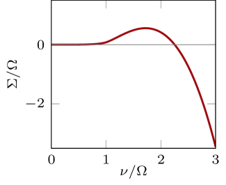
Figure 1: Second order correction to the imaginary part of the effective action for a particle in vacuum, whose internal degree of freedom is a QHO of frequency $\Omega$, and whose center-of-mass exhibits a single-frequency motion of frquency $\nu$.

Above threshold, the second order result is a small correction to the first order one, and combines both DCE and the emission of single photons through excitation-deexcitation process. This correction to the imaginary part of the effective action goes as $-g^{4}(\nu/\Omega)^{3}$ for $\nu/\Omega\gg 1$ (note that the first order result is proportional to $g^{2}(\nu/\Omega)^{3}$ in this limit).

IV Imperfect mirror: microscopic model

Dielectric slabs are in general nonlinear, inhomogeneous, dispersive and also dissipative media. These aspects turn difficult the quantization of a field when all of them have to be taken into account simultaneously. There are different approaches to address this problem. On the one hand, one can use a phenomenological description based on the macroscopic electromagnetic properties of the materials. The quantization can be performed starting from the macroscopic Maxwell equations, and including noise terms to account for absorption. In this approach a canonical quantization scheme is not possible, unless one couples the electromagnetic field to a reservoir, following the standard route to include dissipation in simple quantum mechanical systems. Another possibility is to establish a first-principles model in which the slabs are described through their microscopic degrees of freedom, which are coupled to the electromagnetic field. In this kind of models, losses are also incorporated by considering a thermal bath, to allow for the possibility of absorption of light. There is a large body of literature on the quantization of the electromagnetic field in dielectrics. Regarding microscopic models, the fully canonical quantization of the electromagnetic field in dispersive and lossy dielectrics has been performed by Huttner and Barnett (HB) hb92 . In the HB model, the electromagnetic field is coupled to matter (the polarization field), and the matter is coupled to a reservoir that is included into the model to describe the losses. In the context of the theory of quantum open systems, one can think the HB model as a composite system in which the relevant degrees of freedom belong to two subsystems (the electromagnetic field and the matter), and the matter degrees of freedom are in turn coupled to an environment (the thermal reservoir). The indirect coupling between the electromagnetic field and the thermal reservoir is responsible for the losses. It is well known that if we include the absorption, associated with a dispersive medium, then the dielectric constant will be a complex quantity, whose real and imaginary parts are related by the Kramers-Kronig relations. Losses in quantum mechanics imply a coupling to a reservoir whose degrees of freedom have to be added to the Lagrangian. This suggests that, in order to quantize the vacuum field in a dielectric in a way that is consistent with the Kramers-Kronig relations, one has to introduce the medium into the formalism explicitly. This should be done in such a way that the interaction between light and matter will generate both dispersion and damping of the field. The microscopic theory for the interaction ${\mathcal{S}}_{I}$ between the scalar field and the imperfect mirror, consists of a tern of the form:

$${\mathcal{S}}_{I}^{(m)}(\phi)\;=\;-\frac{1}{2}\int_{x,y}\phi(x)V_{m}(x,y)\phi(y)\;.$$ (43)

The kernel $V_{m}$, is a ‘potential’ resulting from the integration of microscopic degrees of freedom of the polarization field plus the external reservoir. It can be regarded as a symmetric function of $x$ and $y$, since the integrals in ${\mathcal{S}}_{I}$ symmetrize any bi-local function.

We then apply the above discussion to note that the potential $V_{m}$ originated by the interaction between the vacuum field and the imperfect mirror, may also be obtained by a variant of the previous procedure for $V_{p}$; indeed, introducing a bosonic field $Q(t,x^{1},x^{2})$, living on $x^{3}=0$, the plane occupied by the plate, playing the role of the polarization field, also couplet to an external (at equilibrium) environment with degrees of freedom denoted by $q_{n}(t,x^{1},x^{2})$,

$$e^{-\frac{i}{2}\int_{x,y}\phi(x)V_{m}(x,y)\phi(y)}\;=\;\int{\mathcal{D}}Q\;e^{i{\mathcal{S}}^{eff}_{m}(Q,\phi)}\;.$$ (44)

where the effective action ${\mathcal{S}}^{eff}_{m}(Q,\phi)$ is the result of integrating out the degrees of freedom $q_{n}$:

$$e^{i{\mathcal{S}}^{eff}_{m}(Q,\phi)}=\int{\mathcal{D}}q_{n}\;e^{i\left({\mathcal{S}}_{m}(Q,\phi)+{\mathcal{S}}_{m}(Q,q_{n})\right)}\;.$$ (45)

where

$${\mathcal{S}}_{m}(Q,\phi) =\;{\mathcal{S}}_{m}^{(0)}(Q)\,+\,{\mathcal{S}}_{m}^{int}(Q,\phi)\;,$$

$${\mathcal{S}}^{(0)}_{m}(Q) =\;\frac{1}{2}\int dtdx^{1}dx^{2}\,\big{[}(\partial_{t}Q)^{2}-(\Omega_{m}^{2}-i\epsilon)Q^{2}\big{]}\;,$$

$${\mathcal{S}}_{m}^{int}(q,\phi;{\mathbf{r}}) =\;\gamma\,\int dtdx^{1}dx^{2}\,Q(t,x^{1},x^{2})\;\phi(t,x^{1},x^{2},0)\;,$$ (46)

and

$${\mathcal{S}}_{m}(q_{n},\phi) =\;{\mathcal{S}}_{m}^{(0)}(q_{n})\,+\,{\mathcal{S}}_{m}^{int}(Q,q_{n})\;,$$

$${\mathcal{S}}^{(0)}_{m}(q_{n}) =\;\frac{1}{2}\sum_{n}\int dtdx^{1}dx^{2}\,\big{[}(\partial_{t}q_{n})^{2}-(\omega_{n}^{2}-i\epsilon)q_{n}^{2}\big{]}\;,$$

$${\mathcal{S}}_{m}^{int}(Q,q_{n})) =\;\sum_{n}\lambda_{n}\,\int dtdx^{1}dx^{2}\,Q(t,x^{1},x^{2})\;q_{n}(t,x^{1},x^{2})\;.$$ (47)

Here, $\Omega_{m}$ is a frequency, and $\gamma$ determines the coupling, which has the dimensions of $[{\rm mass}]^{3/2}$ (similar happens with $\omega_{n}$ and $\lambda_{n}$). Following Farias:2014wca , microscopic matter degrees of freedom on the mirror, which we assume to occupy the $x^{3}=0$ plane, are assumed to behave as one-dimensional harmonic oscillators, one at each point of the plate. Their generalized coordinates take values in an internal space. Besides, no couplings between the coordinates at different points of the plate are included, and there is a linear coupling between each oscillator and the vacuum field and to the external reservoir.

After integrating out the thermal environment, we obtain an effective action for the internal degrees of freedom into the mirror as

$${\mathcal{S}}^{eff}_{m}(Q)={\mathcal{S}}_{m}^{(0)}(Q)+\int dtdx^{1}dx^{2}Q(t,x^{1},x^{2})K(t,t^{\prime})Q(t^{\prime},x^{1},x^{2}),$$ (48)

where $K(t,t^{\prime})$ is a nonlocal kernel that depends on the temperature and spectral density of the environment. As is well known, for an environment formed by an infinite set of harmonic oscillators at high temperatures with an ohmic spectral density this kernel becomes local and proportional to a dissipation coefficient $\xi$ QBM . In this limit, the effect of the environment on the in-out effective action can be taken into account just replacing $\Omega_{m}^{2}$ by $\Omega_{m}^{2}-i\xi$.

The interaction becomes then local, and $V_{m}$ has the form:

$$V_{m}(x,y)\;\equiv\;\gamma^{2}\;\Delta_{m}(x^{0}-y^{0})\,\delta({\mathbf{x}}-{\mathbf{y}})\;\delta(x^{3})\;,$$ (49)

where $\gamma$ denotes a constant, which is the coupling between the plate harmonic oscillator’s degrees of freedom, and the vacuum field. The precise form of $\Delta_{m}$ is more conveniently expressed in terms of its Fourier transform, namely:

$$\Delta_{m}(x^{0}-y^{0}) =\;\int\frac{d\nu}{2\pi}\,e^{-i\nu(x^{0}-y^{0})}\,\widetilde{\Delta}_{m}(\nu)$$

$$\widetilde{\Delta}_{m}(\nu) \equiv\;\frac{1}{\nu^{2}-\Omega_{m}^{2}+i\epsilon+i\xi}\;.$$ (50)

We would also be interested in the case of a mirror imposing ‘perfect’, i.e., Dirichlet, boundary conditions. Such a case might be obtained by taking particular limits starting from a given $V_{m}$; for example,

$$V_{m}(x,y)\;\to\;V_{D}(x,y)\,\equiv\,\eta\;\delta({\mathbf{x}_{\parallel}}-{\mathbf{y}_{\parallel}})\,\delta(x^{3})\,\delta(y^{3})\;,\;\;\eta\to\infty\;,$$ (51)

where we have adopted the notational convention that, for any spatial vector ${\mathbf{a}}$, ${\mathbf{a}_{\parallel}}\equiv(x^{1},x^{2})$. This Dirichlet limit may be reached from different $V_{m}$ kernels, although it is more convenient, given the simple geometry of the system considered, to use images in order to write the exact scalar field propagator. The same can be said about Neumann boundary conditions, for which the field propagator in the presence of the mirror is also obtained by using images.

V Moving atom in the presence of a plate

In this Section, we deal with contributions which contain both $V_{m}$ and $V_{p}$. We will work here, for the sake of simplicity, always to the first order in $V_{p}$. Therefore, the structure of the term calculated here is as follows:

$$\Gamma_{mp}[{\mathbf{r}}(t)]\;=\;-\frac{1}{2}\,\int_{x,y}V_{p}(x,y)\big{\langle}\phi(x)\phi(y)\big{\rangle}_{m}\;,$$ (52)

where now:

$$\langle\,\ldots\,\rangle_{m}\;\equiv\;\frac{\int{\mathcal{D}}\phi\;\ldots\;e^{i[{\mathcal{S}}_{0}(\phi)-\frac{1}{2}\int_{x,y}\phi(x)V_{m}(x,y)\phi(y)]}}{\int{\mathcal{D}}\phi\;e^{i[{\mathcal{S}}_{0}(\phi)-\frac{1}{2}\int_{x,y}\phi(x)V_{m}(x,y)\phi(y)]}}\;.$$ (53)

In other words, the kind of contribution we consider here, looks like $\Gamma_{p}^{(1)}$, albeit with the free propagator $\big{\langle}\phi(x)\phi(y)\big{\rangle}_{0}$ replaced by the propagator in the presence of the mirror, $\big{\langle}\phi(x)\phi(y)\big{\rangle}_{m}$. The latter may be incorporated either exactly or making some simplifying assumptions, in order to be able to find the imaginary part in an explicit way.

The first non-trivial contribution, which we evaluate, arises when one considers the expansion of the propagator to the first order in $V_{m}$, is:

$$\Gamma^{(1)}_{mp}\;=\;\frac{i}{2}\,\int_{x,y,x^{\prime},y^{\prime}}\,V_{m}(x,y)\,V_{p}(x^{\prime},y^{\prime})\,G(x,x^{\prime})\,G(y,y^{\prime})\;,$$ (54)

$$\Gamma^{(1)}_{mp}\;=\;\frac{i}{2}\,\gamma^{2}\,g^{2}\int\frac{d^{2}{\mathbf{p}_{\parallel}}}{(2\pi)^{2}} \int\frac{dp_{3}}{2\pi}\int\frac{dq_{3}}{2\pi}\int\frac{d\omega}{2\pi}\int\frac{d\nu}{2\pi}\;\Big{[}f({\mathbf{p}_{\parallel}},p^{3},-\omega-\nu)$$

$$\times f(-{\mathbf{p}_{\parallel}},q^{3},\omega+\nu)\; \widetilde{\Delta}_{m}(\omega)\,\widetilde{G}(-\omega,{\mathbf{p}_{\parallel}},p^{3})\,\,\widetilde{\Delta}_{p}(\nu)\,\widetilde{G}(\omega,-{\mathbf{p}_{\parallel}},q^{3})\Big{]}\,$$ (55)

which, by a shift of variables may be written as follows:

$$\Gamma^{(1)}_{mp}\;=\;\frac{1}{2}\,\int\frac{d^{2}{\mathbf{p}_{\parallel}}}{(2\pi)^{2}}\int\frac{dp_{3}}{2\pi}\int\frac{dq_{3}}{2\pi}\int\frac{d\nu}{2\pi}\;f({\mathbf{p}_{\parallel}},p^{3},-\nu)f(-{\mathbf{p}_{\parallel}},q^{3},\nu)\;B(\nu,{\mathbf{p}_{\parallel}},p^{3},q^{3})$$ (56)

where

$$B(\nu,{\mathbf{p}_{\parallel}},p^{3},q^{3})\;=\;i\,\gamma^{2}\,g^{2}\;\int\frac{d\omega}{2\pi}\;\widetilde{\Delta}_{m}(\omega)\,\widetilde{G}(-\omega,{\mathbf{p}_{\parallel}},p^{3})\,\,\widetilde{\Delta}_{p}(\nu-\omega)\,\widetilde{G}(\omega,-{\mathbf{p}_{\parallel}},q^{3})\;.$$ (57)

Introducing the explicit form of the propagator in momentum space, and of the $\widetilde{\Delta}$ functions, we see that:

$$B(\nu,{\mathbf{p}_{\parallel}},p^{3},q^{3})\,=\,-i\,\gamma^{2}\,g^{2} \int\frac{d\omega}{2\pi}\Big{[}\frac{1}{\omega^{2}-\Omega_{m}^{2}+i\epsilon+i\xi}\;\frac{1}{\omega^{2}-{\mathbf{p}_{\parallel}}^{2}-(p^{3})^{2}+i\epsilon}$$

$$\times\frac{1}{(\omega-\nu)^{2}-\Omega_{p}^{2}+i\epsilon}\;\frac{1}{\omega^{2}-{\mathbf{p}_{\parallel}}^{2}-(q^{3})^{2}+i\epsilon}\Big{]}\;.$$ (58)

Since $B(\nu,{\mathbf{p}_{\parallel}},p^{3},q^{3})=B(\nu,{\mathbf{p}_{\parallel}},q^{3},p^{3})$, we conclude that:

$${\rm Im}\big{[}\Gamma^{(1)}_{mp}\big{]} =\;\frac{1}{2}\,\int\frac{d^{2}{\mathbf{p}_{\parallel}}}{(2\pi)^{2}}\int\frac{dp_{3}}{2\pi}\int\frac{dq_{3}}{2\pi}\int\frac{d\nu}{2\pi}\;f({\mathbf{p}_{\parallel}},p^{3},-\nu)f(-{\mathbf{p}_{\parallel}},q^{3},\nu)$$

$$\times\;{\rm Im}\Big{[}B(\nu,{\mathbf{p}_{\parallel}},p^{3},q^{3})\Big{]}\;.$$ (59)

Now we come to the actual evaluation of $B$, which resembles a loop (box) diagram on a $0+1$-dimensional quantum field theory.

Introducing Feynman parameters, and integrating out $\omega$, after a lengthy calculation we find:

$$B(\nu,{\mathbf{p}_{\parallel}},p^{3},q^{3}) =-\frac{\gamma^{2}\,g^{2}}{2\Omega_{p}}\Big{\{}\frac{\Omega_{m}+\Omega_{p}}{\Omega_{m}}\big{[}\frac{1}{p^{2}-\Omega_{m}^{2}+i(\epsilon+\xi)}\frac{1}{q^{2}-\Omega_{m}^{2}+i(\epsilon+\xi)}$$

$$\hskip 56.9055pt\times\frac{1}{\nu^{2}-(\Omega_{m}+\Omega_{p})^{2}+i(\epsilon+\xi)}\big{]}$$

$$-\;\frac{1}{(p^{2}-\Omega_{m}^{2}+i\xi)(q^{2}-p^{2})p}\;\;\frac{p+\Omega_{p}}{\nu^{2}-(p+\Omega_{p})^{2}+i\epsilon}$$

$$-\;\frac{1}{(q^{2}-\Omega_{m}^{2}+i\xi)(p^{2}-q^{2})q}\;\;\frac{q+\Omega_{p}}{\nu^{2}-(q+\Omega_{p})^{2}+i\epsilon}\Big{\}}\;.$$ (60)

Therefore, taking the imaginary part, the $\epsilon\to 0$ limit, and keeping the leading terms when $\xi\to 0$,

$${\rm Im}\big{[}B(\nu,{\mathbf{p}_{\parallel}},p^{3},q^{3})\big{]} =\,\frac{\pi\gamma^{2}g^{2}}{2\Omega_{p}}\Big{\{}\frac{\Omega_{m}+\Omega_{p}}{\Omega_{m}}\,\delta_{\xi}\big{(}\nu^{2}-(\Omega_{m}+\Omega_{p})^{2}\big{)}$$

$$\times\,\big{[}{\mathcal{P}}_{\xi}(p^{2}-\Omega_{m}^{2})\,{\mathcal{P}}_{\xi}(q^{2}-\Omega_{m}^{2})\,- \pi^{2}\delta_{\xi}(p^{2}-\Omega_{m}^{2})\,\delta_{\xi}(q^{2}-\Omega_{m}^{2})\big{]}$$

$$-\frac{p+\Omega_{p}}{p(q^{2}-p^{2})}\;{\mathcal{P}}_{\xi}(p^{2}-\Omega_{m}^{2})\;\delta\big{(}\nu^{2}-(p+\Omega_{p})^{2}\big{)} -\,\frac{q+\Omega_{p}}{q(p^{2}-q^{2})}\;{\mathcal{P}}_{\xi}(q^{2}-\Omega_{m}^{2})\;\delta\big{(}\nu^{2}-(q+\Omega_{p})^{2}\big{)}\Big{\}}\;,$$ (61)

where we have introduced notations for the approximants of Cauchy principal value ${\mathcal{P}}$ and Dirac’s $\delta$-function:

$${\mathcal{P}}_{\xi}(x)\;=\;\frac{x}{x^{2}+\xi^{2}}\;\;,\;\;\;\delta_{\xi}(x)\;=\;\frac{1}{\pi}\,\frac{\xi}{x^{2}+\xi^{2}}\;,$$ (62)

respectively.

The terms retained in (V) above are meant to be the most relevant, when $\xi\to 0$, regarding their contribution to the integrals over frequency and momenta in the imaginary part of the effective action. Besides, we have neglected terms which cancel each other in ${\rm Im}[B]$, in that limit.

On the other hand, note that, besides $\delta_{\xi}$, (V) also contains $\delta$ functions (they arise when taking the $\epsilon\to 0$ limit, and are independent of $\xi$). Using standard $\delta$-function properties (note that, in principle, they are not valid for $\delta_{\xi}$), we see that:

$${\rm Im}\big{[}B(\nu,{\mathbf{p}_{\parallel}},p^{3},q^{3})\big{]}\,=\,\frac{\pi\gamma^{2}g^{2}}{2\Omega_{p}}\Big{\{} \frac{\Omega_{m}+\Omega_{p}}{\Omega_{m}}\,\delta_{\xi}\big{(}\nu^{2}-(\Omega_{m}+\Omega_{p})^{2}\big{)}\,\big{[}{\mathcal{P}}_{\xi}(p^{2}-\Omega_{m}^{2})\,{\mathcal{P}}_{\xi}(q^{2}-\Omega_{m}^{2})$$

$$-\,\pi^{2}\delta_{\xi}(p^{2}-\Omega_{m}^{2})\,\delta_{\xi}(q^{2}-\Omega_{m}^{2})\big{]}$$

$$\,-\,\frac{\theta(|\nu|-\Omega_{p})}{2(|\nu|-\Omega_{p})}\, {\mathcal{P}}_{\xi}\big{(}(|\nu|-\Omega_{p})^{2}-\Omega_{m}^{2}\big{)}\;\big{[}\frac{\delta(p-|\nu|+\Omega_{p})}{q^{2}-(|\nu|-\Omega_{p})^{2}}+\frac{\delta(q-|\nu|+\Omega_{p})}{p^{2}-(|\nu|-\Omega_{p})^{2}}\big{]}\Big{\}}\;.$$ (63)

We identify in (V) the sum of two contributions, with are quite different regarding how and when they turn on, as functions of $\nu$. Indeed, the first one has a $\delta_{\xi}$ function of $|\nu|$ minus the sum of $\Omega_{m}$ and $\Omega_{p}$, while the second one contains a threshold at $|\nu|=\Omega_{p}$. Also, for the latter to contribute, the function $f$ must be non-vanishing when $|\nu|$ surpasses $p$ (or $q$). That will depend, of course, on the nature of the motion considered.

In the following examples, depending on the nature of the motion involved (reflected in $f$), we shall be able to consider the $\xi\to 0$ limit. This will allow us to simplify the expressions as much as possible, namely, depending on the smallest possible number of parameters.

V.1 Quantum friction

The first example the we consider here corresponds to quantum friction, namely, to motion with a constant velocity which is parallel to the plate:

$${\mathbf{r}}(t)\;=\;{\mathbf{r}}_{0}+{\mathbf{u}}\,t\;,$$ (64)

with ${\mathbf{u}}=(u,0,0)$ and ${\mathbf{r}}_{0}=(0,0,a)$. We have:

$$f({\mathbf{p}_{\parallel}},p^{3},\nu)\,=\,2\pi\,e^{-ip^{3}a}\,\delta(\nu-p^{1}u)$$

$$f({\mathbf{p}_{\parallel}},p^{3},-\nu)f(-{\mathbf{p}_{\parallel}},q^{3},\nu)\,=\,e^{-i(p^{3}+q^{3})a}\,T\,2\pi\,\delta(p^{1}u+\nu)\;,$$ (65)

where $T$ denotes the extent of the time interval in the effective action (which, for a constant velocity, must be extensive in time). We see that, since $|u|<1$, $f$ will be non-vanishing only when $|\nu|<p$, and therefore there will not be contributions to the imaginary part coming from the term which has a threshold. Therefore, we shall have:

$$\frac{{\rm Im}[\Gamma^{(1)}_{mp}]}{T} =\;(\Omega_{m}+\Omega_{p})\,\frac{\pi\gamma^{2}g^{2}}{4\Omega_{p}\Omega_{m}}\int\frac{d^{2}{\mathbf{p}_{\parallel}}}{(2\pi)^{2}}\int\frac{dp_{3}}{2\pi}\int\frac{dq_{3}}{2\pi}\int\frac{d\nu}{2\pi}\;e^{-i(p^{3}+q^{3})a}\,2\pi\,\delta(p^{1}u+\nu)$$

$$\,\delta_{\xi}\big{(}\nu^{2}-(\Omega_{m}+\Omega_{p})^{2}\big{)}\,\big{[}{\mathcal{P}}_{\xi}(p^{2}-\Omega_{m}^{2})\,{\mathcal{P}}_{\xi}(q^{2}-\Omega_{m}^{2})\,-\,\pi^{2}\delta_{\xi}(p^{2}-\Omega_{m}^{2})\,\delta_{\xi}(q^{2}-\Omega_{m}^{2})\big{]}\;.$$ (66)

One sees first that the $\xi\to 0$ limit may be safely taken. Moreover, the term which contains the product of three $\delta$-functions vanishes, since their simultaneous contribution requires a frequency which is larger than $p$ or $q$ in modulus.

Thus

$$\frac{{\rm Im}[\Gamma^{(1)}_{mp}]}{T}\;=\;\frac{\pi\gamma^{2}g^{2}}{8\Omega_{p}\Omega_{m}}\int\frac{d^{2}{\mathbf{p}_{\parallel}}}{(2\pi)^{2}}\int\frac{dp_{3}}{2\pi}\int\frac{dq_{3}}{2\pi}\;e^{-i(p^{3}+q^{3})a}\frac{\delta\big{(}|p^{1}u|-(\Omega_{m}+\Omega_{p})\big{)}}{(p^{2}-\Omega_{m}^{2})\,(q^{2}-\Omega_{m}^{2})}\;,$$ (67)

and, integrating out $p^{3}$ and $q^{3}$,

$$\frac{{\rm Im}\big{[}\Gamma^{(1)}_{mp}\big{]}}{T}\;=\;\frac{\pi\gamma^{2}g^{2}}{32\Omega_{p}\Omega_{m}}\,\int\frac{d^{2}{\mathbf{p}_{\parallel}}}{(2\pi)^{2}}\;\frac{e^{-2a\sqrt{{\mathbf{p}_{\parallel}}^{2}-\Omega_{m}^{2}}}}{{\mathbf{p}_{\parallel}}^{2}-\Omega_{m}^{2}}\delta\big{(}|p^{1}u|-(\Omega_{m}+\Omega_{p})\big{)}\;.$$ (68)

We then make use of the remaining $\delta$ function to integrate out $p^{1}$:

$$\frac{{\rm Im}\big{[}\Gamma^{(1)}_{mp}\big{]}}{T}\;=\;\frac{\gamma^{2}\,g^{2}}{32\pi\Omega_{p}\Omega_{m}u}\,\int_{0}^{\infty}dp^{2}\;\frac{e^{-2a\sqrt{(p^{2})^{2}+\frac{1}{u^{2}}(\Omega_{m}+\Omega_{p})^{2}-\Omega_{m}^{2}}}}{(p^{2})^{2}+\frac{1}{u^{2}}(\Omega_{m}+\Omega_{p})^{2}-\Omega_{m}^{2}}\;,$$ (69)

or,

$$\frac{{\rm Im}\big{[}\Gamma^{(1)}_{mp}\big{]}}{T}\;=\;\frac{\gamma^{2}\,g^{2}\,a}{32\pi\Omega_{m}\Omega_{p}}\,\int_{0}^{\infty}dx\;\frac{e^{-\frac{2}{u}\sqrt{x^{2}+a^{2}(\Omega_{m}+\Omega_{p})^{2}-a^{2}u^{2}\Omega_{m}^{2}}}}{x^{2}+a^{2}(\Omega_{m}+\Omega_{p})^{2}-a^{2}u^{2}\Omega_{m}^{2}}\;,$$ (70)

which has the proper dimensions and is consistent with previous results corresponding to friction between planes; in this case the result becomes proportional to the area of the planes, and the dimensionality of the coupling $g$ is different (the same as that of $\gamma$).

V.2 Small oscillations

In this example, we consider an expansion entirely analogous to the one of the free oscillating particle, albeit now in the presence of the plate. We then use the same expansion for the function $f$, namely, $f=f^{(0)}+f^{(1)}+f^{(2)}+\ldots$, with exactly the same terms. Inserting this expansion into the general expression for the imaginary part of $\Gamma_{mp}^{(1)}$, and retaining up to terms of the second order in the departure ${\mathbf{y}}$ from the equilibrium position, we see that the only surviving contribution is the following:

$${\rm Im}[\Gamma^{(1)}_{mp}]=\frac{1}{2}\,\int\frac{d^{2}{\mathbf{p}_{\parallel}}}{(2\pi)^{2}}\int\frac{dp_{3}}{2\pi}\int\frac{dq_{3}}{2\pi}\int\frac{d\nu}{2\pi}f^{(1)}({\mathbf{p}_{\parallel}},p^{3},-\nu)f^{(1)}(-{\mathbf{p}_{\parallel}},q^{3},\nu){\rm Im}[B(\nu,{\mathbf{p}_{\parallel}},p^{3},q^{3})]\;.$$ (71)

Inserting the explicit forms of (V) and $f^{(1)}$ above, we note that we may have contributions due to departures which are parallel or normal to the plane will have a different weight; indeed, the remaining symmetries of the system imply that the structure of the result is:

$${\rm Im}[\Gamma^{(1)}_{mp}]\;=\;\frac{1}{2}\,\int\frac{d\nu}{2\pi}\big{(}\,m_{\shortparallel}(\nu)\,|\tilde{\mathbf{y}}_{\shortparallel}(\nu)|^{2}\,+\,m_{\perp}(\nu)\,|\tilde{y}_{3}(\nu)|^{2}\big{)}\;,$$ (72)

depending on two scalar functions:

$$m_{\shortparallel}(\nu) =\,\frac{1}{2}\,\frac{\pi\gamma^{2}g^{2}}{2\Omega_{p}}\Big{\{}\frac{\Omega_{m}+\Omega_{p}}{\Omega_{m}}\,\delta_{\xi}\big{(}\nu^{2}-(\Omega_{m}+\Omega_{p})^{2}\big{)}$$

$$\times\,\int\frac{d^{2}{\mathbf{p}_{\parallel}}}{(2\pi)^{2}}|{\mathbf{p}_{\parallel}}|^{2} \Big{[}\big{(}\;\int\frac{dp^{3}}{2\pi}\,{\mathcal{P}}_{\xi}(p^{2}-\Omega_{m}^{2})e^{-ip^{3}a}\;\big{)}^{2}\,\,-\,\pi^{2}\big{(}\;\int\frac{dp^{3}}{2\pi}\,\delta_{\xi}(p^{2}-\Omega_{m}^{2})e^{-ip^{3}a}\;\big{)}^{2}\Big{]}$$

$$\,-\,\frac{\theta(|\nu|-\Omega_{p})}{(|\nu|-\Omega_{p})}\, {\mathcal{P}}_{\xi}\big{(}(|\nu|-\Omega_{p})^{2}-\Omega_{m}^{2}\big{)}\;\int\frac{d^{2}{\mathbf{p}_{\parallel}}}{(2\pi)^{2}}|{\mathbf{p}_{\parallel}}|^{2}\,\int\frac{dp^{3}}{2\pi}\int\frac{dq^{3}}{2\pi}\frac{\delta(p-|\nu|+\Omega_{p})}{q^{2}-(|\nu|-\Omega_{p})^{2}}e^{-i(p^{3}+q^{3})a}\Big{\}}\;,$$ (73)

and

$$m_{\perp}(\nu) =\,-\frac{\pi\gamma^{2}g^{2}}{2\Omega_{p}}\Big{\{}\frac{\Omega_{m}+\Omega_{p}}{\Omega_{m}}\,\delta_{\xi}\big{(}\nu^{2}-(\Omega_{m}+\Omega_{p})^{2}\big{)}$$

$$\times\,\int\frac{d^{2}{\mathbf{p}_{\parallel}}}{(2\pi)^{2}} \Big{[}\big{(}\;\int\frac{dp^{3}}{2\pi}\,p^{3}\,{\mathcal{P}}_{\xi}(p^{2}-\Omega_{m}^{2})e^{-ip^{3}a}\;\big{)}^{2}\,\,-\,\pi^{2}\big{(}\;\int\frac{dp^{3}}{2\pi}\,p^{3}\,\delta_{\xi}(p^{2}-\Omega_{m}^{2})e^{-ip^{3}a}\;\big{)}^{2}\Big{]}$$

$$\,-\,\frac{\theta(|\nu|-\Omega_{p})}{(|\nu|-\Omega_{p})}\, {\mathcal{P}}_{\xi}\big{(}(|\nu|-\Omega_{p})^{2}-\Omega_{m}^{2}\big{)}\;\int\frac{d^{2}{\mathbf{p}_{\parallel}}}{(2\pi)^{2}}\int\frac{dp^{3}}{2\pi}\int\frac{dq^{3}}{2\pi}p^{3}\,q^{3}\,\frac{\delta(p-|\nu|+\Omega_{p})}{q^{2}-(|\nu|-\Omega_{p})^{2}}e^{-i(p^{3}+q^{3})a}\,\Big{\}}\;.$$ (74)

After performing the integrals over $p^{3}$ and $q^{3}$, we find for $m_{\shortparallel}$ a more explicit expression:

$$m_{\shortparallel}(\nu) =\,\frac{1}{2}\,\frac{\pi\gamma^{2}g^{2}}{2\Omega_{p}}\Big{\{}\frac{\Omega_{m}+\Omega_{p}}{4\pi\Omega_{m}}\,\delta_{\xi}\big{(}\nu^{2}-(\Omega_{m}+\Omega_{p})^{2}\big{)}\,A_{\shortparallel}(\xi,\Omega_{m},a)$$

$$+\,\frac{1}{8\pi^{2}}\,\theta(|\nu|-\Omega_{p})\,(|\nu|-\Omega_{p})^{2}\,{\mathcal{P}}_{\xi}\big{(}(|\nu|-\Omega_{p})^{2}-\Omega_{m}^{2}\big{)}\;B_{\shortparallel}((|\nu|-\Omega_{p})a)\Big{\}}\;,$$ (75)

with

$$A_{\shortparallel}(\xi,\Omega_{m},a)=\int_{-\Omega_{m}^{2}}^{\infty}\frac{du\,u}{u^{2}+\xi^{2}}\,e^{-2\beta a}\,[u\,\cos(2\alpha a)+\xi\,\sin(2\alpha a)]\,,$$

$$B_{\shortparallel}((|\nu|-\Omega_{p})a)=\int_{0}^{1}du\,[\frac{1-u^{2}}{u}\,\sin(2(|\nu|-\Omega_{p})au)]\,,$$ (76)

and

$$\alpha\equiv\sqrt{\frac{\sqrt{u^{2}+\xi^{2}}-u}{2}}\;\;,\;\;\;\beta\equiv\sqrt{\frac{\sqrt{u^{2}+\xi^{2}}+u}{2}}\;.$$ (77)

In obtaining (V.2), no small-$\xi$ approximation has been made, and the results are shown in Fig. 2 for different values of the parameters of the material (distance to the plate $a$ and frequency $\Omega_{m}$). The plots show a resonant behaviour for $|\nu|=\Omega_{m}+\Omega_{p}$, and the specific shape of this resonance depends on the distance $a$, as we will discuss below.

An entirely similar procedure allows us to find:

$$m_{\perp}(\nu) =\,\frac{\pi\gamma^{2}g^{2}}{2\Omega_{p}}\Big{\{}\frac{\Omega_{m}+\Omega_{p}}{16\pi\Omega_{m}}\,\delta_{\xi}\big{(}\nu^{2}-(\Omega_{m}+\Omega_{p})^{2}\big{)}\,A_{\perp}(\xi,\Omega_{m},a)$$

$$-\,\frac{1}{8\pi^{2}}\,\theta(|\nu|-\Omega_{p})\,(|\nu|-\Omega_{p})^{2}\,{\mathcal{P}}_{\xi}\big{(}(|\nu|-\Omega_{p})^{2}-\Omega_{m}^{2}\big{)}\;B_{\perp}((|\nu|-\Omega_{p})a)\Big{\}}\;,$$ (78)

with $\alpha$ and $\beta$ as in (77) and

$$A_{\perp}(\xi,\Omega_{m},a)=\int_{-\Omega_{m}^{2}}^{\infty}\,du\,e^{-2\beta a}\,\cos(2\alpha a)\,,$$

$$B_{\perp}((|\nu|-\Omega_{p})a)=\int_{0}^{1}du\,u\,\sin(2(|\nu|-\Omega_{p})au)\,.$$ (79)

We show $m_{\perp}$ in Fig. 3 for different characteristics of the materials. The same resonant behaviour is observed near $|\nu|=\Omega_{p}+\Omega_{m}$, and also an oscillatory behaviour that was absent for $m_{\parallel}$. These oscillations have a frequency that depends on the distance to the plate, and their presence is related to the fact that that distance is indeed modified by the center-of-mass motion, in contrast to what happens to the parallel contribution.

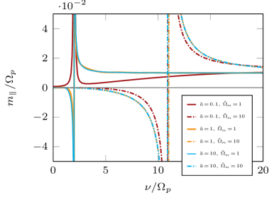
Figure 2: Second order correction to the imaginary part of the effective action, for a particle, modeled as a QHO of frequency $\Omega_{p}$, whose center-of-mass moves with small oscillations of frequency $\nu$, parallel to the plane, at a distance $a$ above it. The plane is modeled as a continuous set of harmonic oscillators of frequency $\Omega_{m}$. We have defined $\tilde{a}=a\Omega_{p}$, $\tilde{\Omega}_{m}=\Omega_{m}/\Omega_{p}$, and we have set the dissipation of the plate as $\xi/\Omega_{p}^{2}=0.01$.

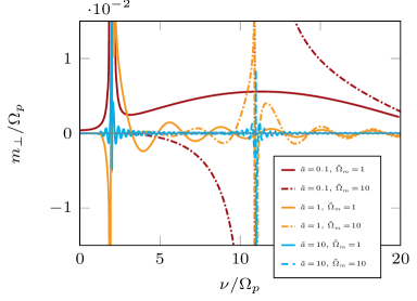
Figure 3: Second order correction to the imaginary part of the effective action, for a particle, modeled as a QHO of frequency $\Omega_{p}$, whose center-of-mass moves with small oscillations of frequency $\nu$ at a distance $a$, normal to a plane. The plane is modeled as a continuous set of harmonic oscillators of frequency $\Omega_{m}$. We have defined $\tilde{a}=a\Omega_{p}$, $\tilde{\Omega}_{m}=\Omega_{m}/\Omega_{p}$, and we have set the dissipation of the plate as $\xi/\Omega_{p}^{2}=0.01$.

The coefficients $B_{\shortparallel}$ and $B_{\perp}$ can be computed explicitly, the result being

$$B_{\shortparallel}(x)=-B_{\perp}(x)+Si(2x)\,,$$

$$B_{\perp}(x)=\frac{-2x\cos(2x)+\sin(2x)}{4x^{2}}\,,$$ (80)

where $Si(x)$ is the sine-integral function.

It is worth noting that there is a qualitative difference in the $a\to\infty$ behaviours of $m_{\shortparallel}$ and $m_{\perp}$ above the $|\nu|>\Omega_{p}$ threshold. Indeed, while the latter vanishes, the former reaches the finite limit:

$$m_{\shortparallel}(\nu)\;\to\;\frac{\gamma^{2}g^{2}}{64\Omega_{p}}\,(|\nu|-\Omega_{p})^{2}\,{\mathcal{P}}_{\xi}\big{(}(|\nu|-\Omega_{p})^{2}-\Omega_{m}^{2}\big{)}\;.$$ (81)

The difference between the response for the two different kinds of oscillations can be traced back to the fact that the respective effective actions depend on different properties of the scalar field propagator in the presence of the plate. Indeed, for parallel motion, one needs the propagator between two points at the same distance $a$ from the plate, while for perpendicular motion one has to take two derivatives with respect the to the third coordinate, and then to evaluate at the average distance, $a$. This results in different $a\to\infty$ limits. Physically, this may be interpreted as a consequence of the different response properties of the plate for normal vs parallel incidence.

We see that, up to this order, the emission probability for both parallel and perpendicular motions is a combination of the approximants of Cauchy’s principal value ${\mathcal{P}}$ and Dirac’s $\delta$-function (see Eq.(62)), both localized at the resonant frequency $|\nu|=\Omega_{m}+\Omega_{p}$. Moreover, in the limit $\xi\to 0$ the coefficients are finite and can be computed explicitly; using the fact that $\alpha\simeq 0$ and $\beta\simeq\sqrt{|u|}$. We obtain:

$$A_{\shortparallel}(0,\Omega_{m},a) = A_{\perp}(0,\Omega_{m},a)=\int_{-\Omega_{m}^{2}}^{\infty}\,du\,e^{-2\sqrt{|u|}a}$$ (82)

$$= \frac{2}{a^{2}}\big{(}2-(1+\Omega_{m}a)e^{-\Omega_{m}a}\big{)}\,.$$

It is interesting to remark that the emission probabilities have peaks at the resonant frequency (with a height determined by he coefficients of the $\delta_{\xi}$ functions) and regions of enhancement and suppression at both sides of the resonant frequency, with amplitudes given by the coefficients that multiply the principal values. The ratio of the coefficients of $\delta_{\xi}$ and ${\mathcal{P}}_{\xi}$ in Eqs.(V.2) and (V.2) determine, for each kind of motion, which is the dominant behaviour. We illustrate this in Fig. 4.

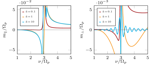
Figure 4: Second order correction to the imaginary part of the effective action for $\Omega_{m}/\Omega_{p}=2$. We show the behaviour near the resonance, that occurs at $|\nu|=\Omega_{m}+\Omega_{p}$. We have defined $\tilde{a}=a\Omega_{p}$.

The structure of the results is reminiscent to what happens with the spontaneous decay rate of an excited atom immersed in an absorbing dielectric spontaneous . Note also that the dissipation coefficient $\xi$ regulates the otherwise infinite results that would be obtained for non-lossy dielectrics. In the electromagnetic case, the presence of $\xi$ insures the validity of the Kramers-Kronig relation. For the particular case ($\xi=0$), one should work beyond the perturbative approximation in the interaction between the mirrors’ degrees of freedom and the quantum field. In our case, the atom is outside the dielectric, and the corrections to the free space probability of emission are due to the vacuum fluctuations that are present near the surface of the dielectric plane Bartolo .

VI Conclusions

We have calculated the vacuum persistence amplitude for a moving harmonic oscillator, first in free space, and afterwards in the presence of a dielectric plane. The in-out effective action was perturbatively evaluated, in an expansion in powers of the coupling between the atom and the field. We presented the result for the corresponding imaginary part as a functional of the atom’s trajectory, showing that, to the lowest non trivial order, there is a threshold. This is associated to the possibility of internal excitation of the atom, before radiation emission. We also found that the NTLO exhibits the combination of the previously mentioned effect with the usual DCE (which does not involve such excitation process). An interesting point of the calculation is the shift in the natural frequency of the oscillator (and therefore in the energy levels of the atom) produced by the vacuum fluctuations. It is mandatory to take into account this shift in order to obtain finite corrections to the vacuum persistence amplitude at the NTLO. Further, we have considered the motion of the atom in the presence of an imperfect mirror, considering quantum harmonic oscillators as microscopic degrees of freedom coupled to an environment as a source of internal dissipation. Again, we have evaluated the vacuum persistence amplitude for the case of an atom moving near the plate, up to first order in both couplings between the atom and the microscopic degrees of freedom and the vacuum field. We have shown that, at the same order in which there is DCE, there also is quantum contactless friction and corrections to free emission. These corrections show a peculiar behaviour when the external frequency equals the sum of the frequency of the atom and the frequency of the microscopic degrees of freedom, with regions of enhancement and suppression of the vacuum persistence amplitude. We pointed out that this is similar to what happens with the spontaneous emission of an atom immersed into a lossy dielectric. The inclusion of losses in the dielectric is crucial to get a finite vacuum persistence amplitude for an accelerated motion of the atom. Friction effects are less sensitive to dissipation, and have a well defined limit for non-lossy dielectrics.

VII Acknoweledgements

This work was supported by ANPCyT, CONICET, UBA and UNCuyo; Argentina. M. B. Farías acknowledges financial support from the national Research Fund Luxembourg under CORE Grant No. 11352881.

References

(1) V. V. Dodonov,
Phys. Scripta 82, 038105 (2010);
D. A. R. Dalvit, P. A. Maia Neto and F. D. Mazzitelli,
Lect. Notes Phys. 834, 419 (2011);
P. D. Nation, J. R. Johansson, M. P. Blencowe and F. Nori,
Rev. Mod. Phys. 84, 1 (2012).
(2) A. Volokitin and B. N. Persson, Reviews of Modern Physics 79, 16 (2007); J. Pendry, Journal of Physics: Condensed Matter 9, 10301 (1997; J. Pendry, New Journal of Physics 12, 033028 (2010).
(3)
M. B. Farías, C. D. Fosco, F. C. Lombardo, F. D. Mazzitelli and
A. E. Rubio López,
Phys. Rev. D 91, 105020 (2015).
(4) Ludmila Viotti, M. Belén Farías, Paula I. Villar, and Fernando C. Lombardo, Phys. Rev. D 99, 105005 (2019).
(5) C.R. Galley, R.O. Behunin and B.L. Hu, Phys. Rev. A 87, 043832 (2013).
(6) R. de Melo e Souza, F. Impens, P.A. Maia Neto
Phys. Rev. A 97, 032514 (2018).
(7) L. Lo and C. K. Law
Phys. Rev. A 98, 063807 (2018).
(8) A. Raval, B. L. Hu and J. Anglin, Phys. Rev. D 53, 7003
(1996);
S.-Y. Lin and B. L. Hu, Phys. Rev. D 76, 064008 (2007); J. Doukas,
S. Y. Lin, B. L. Hu, R. B. Mann, JHEP 11, 119 (2013); S.Y. Lin, JHEP 11, 102 (2017); S.-Y. Lin, Phys. Rev. D 98, 105010 (2018).
(9)J. Klatt, M.B. Farías, D.A.R. Dalvit, and S.Y. Buhmann, Phys. Rev. A 95, 052510 (2017).
(10) F.D. Mazzitelli, J.P. Paz, and A. Villanueva
Phys. Rev. A 68, 062106 (2003).
(11) F. Impens, C. Ccapa Ttira, R.O. Behunin, P.A. Maia Neto, Phys. Rev. A 89 , 022516 (2014).
(12) A. Belyanin, V. Kocharovsky, V. Kocharovsky and F. Capasso, Phys. Rev. Lett. 88, 053602 (2002).
(13) E. Alvarez and F.D. Mazzitelli,
Phys. Rev. A 77, 032113 (2008).
(14) M. Antezza, C. Braggio, G. Carugno, A. Noto, R. Passante, L. Rizzuto, G. Ruoso and S. Spagnolo,
Phys. Rev. Lett. 113, 023601 (2014); F. Armata, R. Vasile, P. Barcellona, S. Y. Buhmann, L. Rizzuto and R. Passante,
Phys. Rev. A 94, 042511 (2016).
(15) B. Huttner and S. M. Barnett, Phys. Rev. A 46, 4306 (1992).
(16) B. L. Hu, J. P. Paz and Y. Zhang,
Phys. Rev. D 47, 1576 (1993).
(17) S.M. Barnett, B. Huttner, and R, Loudon,
Phys. Rev. Lett. 68, 3698 (1992); S.M. Barnett et al, J. Phys. B: At. Mol. Opt. Phys. 29 3763 (1996).