The Informativeness of Estimation Moments††thanks: We gratefully acknowledge financial support from the National Science Foundation (grant numbers SES-1530741 and SES-1824131), the Danish Council for Independent Research in Social Sciences (FSE, grant no. 4091-00040), the ESRC through the Centre for Microdata Methods and Practice (RES-589-28-0001) and the ERC (SG338187). The activities of Center for Economic Behavior and Inequality (CEBI) are financed by a grant from the Danish National Research Foundation. We thank Sharada Dharmasankar, the coeditor and three anonymous referees for constructive comments and suggestions. A previous version of this paper was distributed under the title “Sensitivity of Estimation Precision to Moments with an Application to a Model of Joint Retirement Planning of Couples.”
Abstract
This paper introduces measures for how each moment contributes to the precision of parameter estimates in GMM settings. For example, one of the measures asks what would happen to the variance of the parameter estimates if a particular moment was dropped from the estimation. The measures are all easy to compute. We illustrate the usefulness of the measures through two simple examples as well as an application to a model of joint retirement planning of couples. We estimate the model using the UK-BHPS, and we find evidence of complementarities in leisure. Our sensitivity measures illustrate that the estimate of the complementarity is primarily informed by the distribution of differences in planned retirement dates. The estimated econometric model can be interpreted as a bivariate ordered choice model that allows for simultaneity. This makes the model potentially useful in other applications.
Keywords: Parameter Sensitivity, GMM, Ordered Models, Retirement, Externalities.
JEL Code: C01, C13, C35, J32.
1 Introduction
Indirect inference and other nonlinear GMM estimators are used extensively in empirical research. These estimators are, however, sometimes seen as black boxes. It can be difficult to understand exactly what features of the data are informative about which parameters, and how sensitive parameter estimates are to moments included in the objective function.
In this paper, we provide simple and easy-to-compute measures that can indicate how altering the moments used in estimation affects the precision of parameter estimates. Informally, we think of these as measures of how informative each moment is about a particular parameter. More precisely, we provide measures of the effect on asymptotic standard errors from i) a marginal increase in the noise associated with a moment, ii) completely removing a (set of) moments from estimation, and iii) a marginal increase in the weight put on a moment.
The measures are derived from the asymptotic distribution of the class of GMM-type estimators considered here and are, for the most part, based on derivatives of the asymptotic covariance matrix. The measures are almost costless to calculate because most of the required quantities are already constructed when calculating asymptotic standard errors. Furthermore, the measures have straightforward interpretations if scaled in a meaningful way.
There is a growing literature investigating sensitivity of estimators in economics. Recently, for example, \citeasnounAndrewsGentzkowShapiro2017_sensitivity proposed a measure to inform researchers on the sensitivity of the asymptotic bias in estimators to misspecification of moments included in the estimation function. We note that their measure is also related to the change in the asymptotic variance from a marginal change in the included moments, which inspired our proposed alternative measures. While we focus on the precision of the parameter estimates, more recently \citeasnounArmstrongKolesar2018 and \citeasnounBonhommeWeidner2018 have also studied local misspecification. \citeasnounChristensenConnault2019 studied global misspecification.
We illustrate the applicability of our measures through two simple examples and an empirical application. The two examples are a binary outcome probit model and a proportional hazards Weibull duration model with time-varying covariates. The application is a simple structural model of joint retirement planning of dual-earner households. The model is founded in utility maximization with household bargaining, but can also be interpreted as a bivariate ordered choice model that allows for simultaneity. The parameters of the model are most easily estimated by indirect inference, but the complexity of the model makes it difficult to understand the link between the data and the parameter estimates.
While a growing empirical literature has established that dual earner households tend to retire simultaneously or in quick succession in age,111See e.g. \citeasnounHurd1990; \citeasnounBlau1998; \citeasnounGustmanSteinmeier2000; \citeasnounGustmanSteinmeier2004; \citeasnounCoile2004; \citeasnounAnChristensenGupta2004; \citeasnounJia2005; \citeasnounBlauGilleskie2006; \citeasnounvanderKlaauwWolpin2008; \citeasnounBanksBlundellCasanova2010; \citeasnounCasanova2010 and \citeasnounHonorePaula2018. the empirical evidence of joint retirement planning of couples is much more scarce and with ambiguous findings.222See \citeasnounPientaHayward2002; \citeasnounMoenHuangPlassmannDentinger2006; and \citeasnoundeGripFouargeMontizaan2013. We contribute to this literature by estimating a structural model of dual-earner retirement planning using indirect inference and prospective retirement planning questions in the British Household Panel Survey (BHPS). Our estimation results support the notion of leisure complementarities in retirement. Our proposed sensitivity measures confirm the intuition that the parameter estimate measuring leisure complementarities in the model is sensitive to the distribution of the difference in the year of planned retirement between household members.
2 Framework and Sensitivity Measures
Indirect inference and other nonlinear GMM estimators are sometimes seen as black boxes where it can be difficult to understand exactly what features of the data are informative about which parameters. In this section, we review and introduce a number of measures that are meant to provide information about this.
To fix ideas, consider a set of moment conditions , where is data for observation and it is assumed that this defines a unique . The generalized method of moments (GMM) estimator of is , where is a symmetric, positive definite matrix. While some of the measures below also apply to just-identified models, we focus here on over-identified models where the number of moments are larger than the number of parameters in , and the weighting matrix thus plays a role.
Subject to the standard regularity conditions, the derivation of the asymptotic distribution of gives
| (1) |
where and is the limit of . See \citeasnounHansen1992. The limiting distribution of the GMM estimator is
where
and under random sampling. If we use the optimal weighting matrix, , the asymptotic covariance collapses to
Intuitively, when there is little sampling variability in the moment functions, , will be small. is larger if the moment condition is more sensitive to perturbations in the parameter. Both of these contribute to the precision of the estimates as the proposed measures highlight.
AndrewsGentzkowShapiro2017_sensitivity proposed the sensitivity measure
It is clear from (1) that provides the mapping from moment misspecification of the type into parameter biases for small . Alternatively, by noting that , tells us how additional noise in each of the sample moments would result in additional noise in each element of . This is what motivates our alternative measures that address the sensitivity of estimation precision to each moment.
The proposed measures are intended to complement the measure of sensitivity to misspecification proposed by \citeasnounAndrewsGentzkowShapiro2017_sensitivity. Like , our measures are matrices where the ’th element provides an answer to how the precision of the ’th element of depends on the ’th moment.
Our first measure asks the hypothetical question: How much precision would we lose if the ’th moment is subject to a little additional noise? This measure is formally defined as
where is a matrix with 1 in the element and zero elsewhere. This measure assumes that the optimal weighting matrix is used and updated. Alternatively, we could ask the same question keeping the (possibly non-optimal) weighting matrix unchanged. This measure is
The difference between and is that the former evaluates the potential information in each moment while the latter evaluates the information actually used in the estimation. With efficient GMM (so ), equals . This is also true in the just-identified case where the number of moments equals the number of parameters to be estimated.
Related to , we could consider the change in the asymptotic variance from completely excluding the ’th moment,
where
Here denotes element-wise multiplication and is a vector with ones in all elements except the ’th element, which is zero. leaves the weighting matrix on the remaining moments unchanged after we have excluded the ’th moment.
We note that this measure assumes that the parameter vector is identified after the ’th moment has been excluded. Specifically, needs to have full rank. Importantly, this means that the original model has to be over-identified in the sense that it has more moments than parameters. In practice, has to be estimated, and violations of the full rank assumption will result in being close to singular. Extremely large values in the estimate of therefore suggest that the model is not point-identified when the ’th moment is excluded. This can happen even if the original model was over-identified.
Alternatively, one could also consider measures that adjust the weighting matrix. For example, one could consider a measure that compares the precision of the optimal GMM estimator that uses all moments to the optimal GMM estimator that excludes that ’th moment,
where is the same as matrix except that the ’th row has been removed, and is with the ’th row and column removed. This measure also assumes that the parameter vector is identified after the ’th moment has been excluded, and it implicitly assumes that the original number of moment conditions exceeds the number of parameters to be estimated.
and can also be used to gauge the sensitivity of the estimator to a set of moments. This is potentially useful in cases where one can group moments in some natural way. One can then address the question of how much of the precision in an estimator would be lost if one did not use one of the groups of moments. For example, \citeasnounGayleShephard2019 talks about five sets of moments (in their online appendix), and \citeasnounHonorePaula2018 get their moments from the estimation of four different auxiliary reduced form models. A reparameterization of those reduced form models would lead to moment conditions which are (asymptotically) linear combinations of the original moment conditions. In that case, it might be useful to construct a measure that reflects giving zero weight to all the moments that come from a specific auxiliary model. This approach would be application-specific, and we therefore do not pursue it in this paper.
Our final measure addresses the question: How would the precision of our estimates change if we slightly increased the weight put on the th moment? This measure is formally defined as the derivative
We do not think of as a measure of moment sensitivity, but rather as a measure of how close the chosen weighting matrix is to being optimal. will be 0 when is the optimal weighting matrix. It will also be 0 in the just-identified case, where the number of moments equals the number of parameters to be estimated.
These measures are not invariant to scale of the included moments in . One approach, which we take, is to report scaled measures. Concretely, we report the sensitivity of the ’th parameter to the ’th moment as
Note that , and are elasticities whereas and are the relative changes in the asymptotic variance compared to the baseline with all moments included.
3 Examples
In this section, we illustrate the use of our proposed measures through two concrete examples. The first example is a simple binary choice probit model and the second example is a proportional hazards duration model. The first example is chosen because it is a case where one would have a strong prior about which moments matter. The second example, on the other hand, is complicated enough that this is not obvious.
For both examples, we use both the optimal weighting matrix and a diagonal weighting matrix with the inverse of the moment variances on the diagonal. We chose the latter non-optimal weighting matrix because it is very common in empirical applications.333There are many examples of this. This includes \citeasnounEisenhauerHeckmanMosso2014 and \citeasnounGayleShephard2019 to name two. The motivation stems from \citeasnounAltonjiSegal1996 who show that the optimal weighting matrix can have quite poor finite sample properties. They suggest equally weighted moments (i.e., ) as an alternative. Of course, using equal weights will not be invariant to changes in units (or other rescaling), which explains the practice we have adopted.
3.1 Example 1: Method of Moments Estimation of a Probit Model
We first consider a simple probit model
where has a bivariate normal distribution with means equal to 0, variance 1 and correlation 0.5. is independent of and distributed according to a standard normal. We set . This makes and .
We consider the asymptotic distribution of a moment-based estimator of solving
where we use the six moments
and . In the corresponding logit model, the first three moments correspond to the first order conditions for maximum likelihood estimation. Although they are formally different, the logit and probit models are quite similar. We therefore expect the first three moments to be the most informative about . Moreover, we expect the first moment to be the most important for determining , and the second and third for determining and , respectively.
Table 1 shows results using the optimal weighting matrix and Table 2 shows results using the diagonal weighting matrix with the inverse of the moment variances on the diagonal.444We illustrate the proposed sensitivity measures through Monte Carlo simulation of the expected values using simulated observations. We think of the latter as a practical alternative to the efficient weighting matrix.
It is clear from Table 1 that the first three moments are indeed the most informative about , and , respectively. As mentioned, this is expected since these moments would be the first order conditions for maximum likelihood estimation of a logit model.
The elements in the last three columns of in Table 1 are much smaller than the elements in the first three. This suggests that the optimal GMM estimator is much less sensitive to misspecification of the last three moments than to misspecification of the first three moments. The reason is that the first three moments get almost all the weight (in the corresponding logit model, they would literally get all the weight). As expected, this is less pronounced in Table 2. The values of in Tables 1 and 2 confirm that the efficient GMM estimator of is driven by the first three moments.555 in Tables 1 and 2 differ only because of simulation error. Adding noise to the last three moments has essentially no effect on the precision of the optimal GMM estimator of , whereas adding noise to the first three elements can have a big effect. The values of in Table 2 illustrate that the precision of the non-optimal GMM estimator is less sensitive to noise in the last three moments (because they get relatively less weight) and more sensitive to adding noise to the first three moments (because they get relatively more weight).
Next, and suggest that leaving out, for example, the second moment would increase the asymptotic variance of both the efficient and the inefficient GMM estimator of by around 400 percent. This confirms that is instrumental for precise estimation of .
The final measure, in Table 1 is 0 by construction. Since we are using the weighting matrix that minimizes the variance of the estimator of each element of , the derivative of the variance with respect to the elements of the weighting matrix must be 0. in Table 2 shows that in this case, the diagonal weighting matrix with the inverse of the moment variances on the diagonal puts too little weight on the first three moments.
3.2 Example 2: Duration Model
The probit example in Section 3.1 was chosen because it is an example where we have good prior intuition about which moments matter for what parameter. We now turn to an example where this is much less obvious.
Consider a duration, , which follows a mixed proportional hazard model with time-varying covariates and a Weibull as the baseline hazard
where is the scale parameter which captures duration dependence and is the effect of the time-varying explanatory variables. An example of a two-dimensional time-varying set of explanatory variables could be
Finally, captures unobserved heterogeneity. Except for moment assumptions, no assumptions are made on the distribution of .
We then have the survival function for ,
Since
we have
or
| (2) |
Here, denotes an exponentially distributed random variable with mean 1, and follows a standard Gumbel distribution with (Euler’s constant) and .
Equation (2) suggests moment conditions of the type
| (3) |
for functions of the covariates, . Here, captures the mean of which is assumed to be finite.
When is time-invariant, (2) becomes
or
In other words, with time-invariant covariates the moments implied by (3) do not identify , but only . It turns out that it is possible to estimate by other methods (see, for example, \citeasnounhonore1990), but it is not possible to estimate at the usual rate (see \citeasnounHahn1994). This makes it interesting to investigate how precision in estimation of depends on the various moments in (3) when does contain time-varying covariates.
We consider a data generating process with one time-invariant and one time-varying covariate. Specifically, where
with , , and . through follow standard normal distributions. The heterogeneity term, , follows a log-normal distribution, where the underlying normal has mean 0 and variance . is independent of . Finally, and . With this, the median duration is approximately 1.3, approximately 38% of the durations are less than 1, and 29% greater than 2. This design is chosen because it is a simple example with sizable unobserved heterogeneity and duration dependence, and where we expect that the time-varying covariate might have bite. The design is not meant to mimic any realistic empirical example.
We again consider a moment-based estimator of solving
where we use the five moments given by (3) with .
The sensitivity measures are given in Tables 3 and 4. In this design, the derivative of the first two moments at the true parameter values are non-zero with respect to and , respectively. The derivatives are 0 with respect to the other parameters. This implies that becomes singular when we exclude either of the first two moments. This explains the extreme entries for and in Tables 3 and 4.
The conclusions from the remaining parts of the sensitivity measures are fairly consistent. Most interestingly, the moments formed on the basis of the time-varying covariates contribute to the identification of , while the moment based on the time-invariant covariate does not. This is exactly what the discussion above would predict. Interestingly, the first moment is also important for . Presumably, this is because this moment determines the estimate of the mean of the (log of the) unobserved heterogeneity. It is well-known in the duration literature that unobserved heterogeneity is poorly distinguished from duration dependence. As a result, we do not consider this surprising.
4 Application: Joint Retirement Planning
In this section, we apply the proposed sensitivity measures to an extremely simple structural model of the joint retirement planning of dual-earner couples.
4.1 Data and Institutional Setting
We use the British Household Panel Survey (BHPS), which is a completed panel of 18 waves collected from 1991 through 2009. In waves 11 and 16 of the BHPS, each adult household member is asked, “Even if this is some time away, at what age do you expect you will retire?” We use this to measure the subjective retirement plans of each spouse.666The exact formulation in wave 11 is slightly different:“At what age do you expect to retire/will you consider yourself to be retired?” Based on the age at the interview and the expected retirement age, we can calculate the expected retirement year of each household member and use that to investigate joint retirement plans.
Besides retirement plans, we use information in the BHPS on annual labor market income, the number of visits to the general practitioner (GP), subjective expectations about future health status, eligibility for an employer provided pension scheme (EPP), and whether individuals save any of their income in a private personal pension (PPP).777The EPP includes both defined and contributed benefit (DB and CB) plans and we cannot distinguish between them. \citeasnounBlundellMeghirSmith2004 show, however, that DB plans were most common in the U.K. in this period. Finally, we define individuals as highly skilled if they have completed the first or second stage of tertiary education (ISCED codes 5 or 6).
We use information on households consisting of two opposite-sex household members who are either married or cohabiting, and who meet the following sample selection criteria: i) Both members are between 40 and 59 years old when interviewed, ii) At least one member is not retired at the time of the interview, and iii) Retirement plans are observed in the age range 50 to 70 for at least one member not retired at the time of the interview. If a household satisfies the criteria in both waves (11 and 16), we use both survey responses in the analysis. We refer to each household member as husband or wife, although we also include households, where couples are cohabiting, but not necessarily married.
The State Pension Age (SPA)
The state pension age (SPA) in the U.K. is the age where individuals become eligible to receive state pension from the government. Individuals who have reached SPA and contributed to the scheme for sufficiently many years are eligible to receive a weekly transfer with no means testing. In 2009, the weekly rate was around . See \citeasnounBozioCrawfordTetlow2010, \citeasnounBlundellMeghirSmith2004 and \citeasnounCribbEmmersonTetlow2013 for excellent descriptions of the pension system in the U.K.
The SPA was 65 for men and 60 for women until the implementation of the Pension Act 1995. The Pension Act 1995 introduced an increase in the SPA of women born after April 6, 1950. While the SPA for men was unaffected, the SPA for women was gradually increased by one month every month (by date of birth) until the SPA for women reached 65 for cohorts born later than (including) 1955. See \citeasnounThurleyKeen2017 for a comprehensive discussion of the reform.888After the relevant waves in the BHPS (11 and 16) were conducted, the Pension Act 2007 further increased the SPA for both men and women. Since the respondents were interviewed before this reform was passed (most interviews was done no later than 2006), we abstract from this and other subsequent reforms. Since this might affect individual expectations, our modelling framework explicitly allows for an effect of the Pension Act 1995 on retirement planning.
Descriptive Statistics
Table The Informativeness of Estimation Moments††thanks: We gratefully acknowledge financial support from the National Science Foundation (grant numbers SES-1530741 and SES-1824131), the Danish Council for Independent Research in Social Sciences (FSE, grant no. 4091-00040), the ESRC through the Centre for Microdata Methods and Practice (RES-589-28-0001) and the ERC (SG338187). The activities of Center for Economic Behavior and Inequality (CEBI) are financed by a grant from the Danish National Research Foundation. We thank Sharada Dharmasankar, the coeditor and three anonymous referees for constructive comments and suggestions. A previous version of this paper was distributed under the title “Sensitivity of Estimation Precision to Moments with an Application to a Model of Joint Retirement Planning of Couples.” reports the descriptive statistics for the variables that we use. All statistics are based on households in which both members are not retired at the time of the interview, which is around 97 percent of our sample. Husbands in the estimation sample are approximately 1.5 years older than their wives, plan to retire two years later than their wives (at age 63 on average), and the average difference in the planned retirement year is approximately 0.83 years. This difference should be viewed in light of the fact that the SPA of men is 65, while it is substantially lower for most women in our sample and as low as 60 for women born before 1950. To illustrate simultaneous retirement planning, Figure 1 shows the distribution of the difference in the planned year of retirement between husband and wife. The left panel illustrates the unconditional distribution and the right panel conditions on the husband being at least 2 years older than his wife. The peak around zero indicates joint retirement planning, and the mass to the right of zero likely stems from men being older than women and women having a lower SPA. When conditioning on the husband being at least 2 years older than his wife in the right panel, we see a substantial mass at 0 (same planned retirement year); we now also see a substantial mass at (same planned retirement age).
Table The Informativeness of Estimation Moments††thanks: We gratefully acknowledge financial support from the National Science Foundation (grant numbers SES-1530741 and SES-1824131), the Danish Council for Independent Research in Social Sciences (FSE, grant no. 4091-00040), the ESRC through the Centre for Microdata Methods and Practice (RES-589-28-0001) and the ERC (SG338187). The activities of Center for Economic Behavior and Inequality (CEBI) are financed by a grant from the Danish National Research Foundation. We thank Sharada Dharmasankar, the coeditor and three anonymous referees for constructive comments and suggestions. A previous version of this paper was distributed under the title “Sensitivity of Estimation Precision to Moments with an Application to a Model of Joint Retirement Planning of Couples.” also shows that around 16 and 14 percent of men and women, respectively, are classified as highly skilled, and we see that men tend to visit the GP much less than women. Interestingly, however, men are more likely to expect their health to worsen in the future. The labor income of husbands is around while that of the wives is on average around . Only around 13 percent of wives and 28 percent of husbands contribute to a private pension (PPP), while around 47 percent of wives and 51 percent of husbands are eligible to some occupational retirement scheme (EPP).
4.2 A Model of Retirement Planning of Dual-Earner Households
In this section, we formulate a discrete time version of the continuous time bivariate duration model proposed in \citeasnounHonorePaula2018. Specifically, we parameterize the difference in the utility flow between being retired and working. Utility maximization then gives an estimatable model for joint retirement planning of couples.
Consider first the husbands. We specify the difference in utility from being retired in period compared to working as
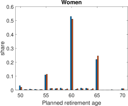
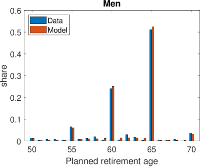
where is the calendar time, is the retirement age of the wife, and thus is the calendar time at which the wife plans to retire. We interpret the term as a utility externality that allows the husband to enjoy a higher utility flow from planned retirement if the wife also plans to be retired at that time. We parameterize the planned retirement age function, , as a linear trend plus indicator functions for , and . The histograms in Figure 2 below suggest that these are empirically important. We interpret the first two as reflecting either social norms or heaping, while the third also reflects the fact that the SPA for men is 65.
Similarly, the difference in utility flow for the wife is
We again parameterize the function as a linear trend plus indicator functions for , and . The term reflects the idea that for women, there is variation in the SPA as discussed above. This allows one to infer the effect of the SPA separately from the dummies that reflect either heaping or institutional features (e.g., early and statutory retirement ages) at 55, 60 and 65.
To close the model, we assume that is jointly normal with mean zero and covariance matrix , where the off-diagonal element of captures possibly correlated retirement preferences within households. We also assume that retirement is an absorbing state. When the difference in utility from retirement compared to working is increasing in age, this is not a binding constraint in the sense that individuals would not want to re-enter the labor market once retired.
If a husband and a wife plan to retire at ages and , their discounted individual utilities are
for a husband aged and
for a wife aged . Finally, the optimal retirement plan for a household is determined jointly as
where is a household aggregator. For the estimation, we choose as in the Nash bargaining setting from \citeasnounHonorePaula2018 or, more generally, the collective model framework surveyed in \citeasnounBrowningChiapporiWeiss2014.
It is clear that two scale normalizations are necessary in order to estimate the model. First, the scale of cannot be identified and we therefore normalize the variance of to be . Secondly, the only effect of is to re-scale all the parameters in . We therefore normalize . The model is thus in effect unitary.
Our parameterization is inspired by the ordered probit model. Consider the husbands. If (such that there is no utility externality) and is increasing, then the utility maximation will lead to planned retirement the first time . In other words, the chosen planned retirement age satisfies
which is exactly the ordered probit model. In that sense, the proposed model is a generalization of the ordered probit model to a bivariate case with simultaneity between the two outcomes.
4.3 Indirect Inference Estimation
We estimate the model’s parameter vector through indirect inference999See, for example, \citeasnounsmith1993, and \citeasnounGourierouxMonfortRenault1993. While we use the Wald criterion function, indirect inference can also be performed using other metrics (for example, the likelihood ratio or Lagrange multiplier). See \citeasnounSmith2008.,
The weighting matrix, , is diagonal with the inverse of the variances of the moments in the diagonal. is a vector of differences between statistics/moments in the data and identical moments based on simulated data.
For each couple , we simulate synthetic retirement plans by drawing vectors of taste shocks from the joint normal distribution and calculate the value of all combinations of retirement ages
where the individual values are calculated as in (LABEL:eq:Vh) and (LABEL:eq:Vw). We then find the simulated retirement ages that maximize utility,
for a given value of .
To estimate the model parameters, we use four sets of auxiliary models/moments with a total of elements in . We describe in detail the construction of these moments in the supplemental material and only list them here:
-
1.
OLS coefficients from individual regressions of the planned retirement age on own and spousal covariates and together with indicators for the wife’s birth cohort and .
-
2.
The share of individuals planning to retire at ages 50-54, 55, 56-59, 60, 61-64, and 65, split by gender.
-
3.
The covariance matrix of residuals from the regression in bullet 1 above for each household member.
-
4.
The share of couples with retirement plans such that i) the wife plans to retire 1–2 years before her husband, ii) the husband plans to retire 1–2 years before his wife, or iii) the couple plan to retire in the same year.
The first set of moments are primarily included to help estimate , , and in the utility function. The second set of moments are included primarily to help estimate the linear age trend and age dummies in and . The third set of moments are primarily included to estimate the covariance of the preference shocks for husband and wife, . Recall that we normalize and the remaining parameters in are thus and . The final set of moments are included to estimate the value of joint leisure, . We will use our proposed sensitivity measures below to investigate these claims in a more systematic way.
4.4 Empirical Results
We use the BHPS data discussed above to estimate the model of joint retirement planning of couples. We use the same moments as above and simulate draws when approximating the expected moments. Table 6 reports the estimation results. We find a positive value of coordination of around , around two to four times as large as the marginal utility from additional labor income of and significant at the level (p-value of ).
Overall, the remaining statistically significant parameter estimates have the expected signs. High skilled individuals value retirement less. Less healthy people value retirement more, and having some form of pension savings increase the value of retirement. Having an employer provided pension (EPS) especially increases the utility from retirement compared to working for husbands. Perhaps surprisingly, we find that higher earning women value retirement more but this could proxy for higher wealth, which could lead to a higher propensity to retire. All spousal variables seem to matter less and are not statistically significant at most common significance levels. Interestingly, we estimate a small positive and insignificant increase in the expected retirement age of women in response to an increased SPA. This goes in line with other studies finding a relatively low degree of awareness of the reform (\citeasnounCrawfordTetlow2010).
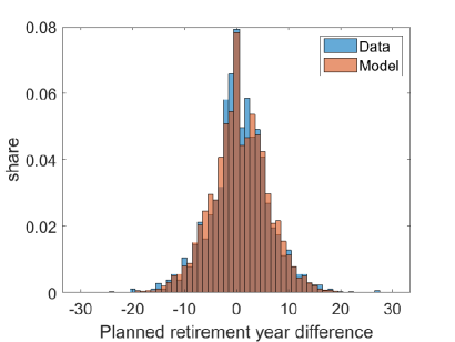
Figure 2 shows the histogram of planned retirement ages for women and men. We see that the model does a quite good job fitting the empirical distribution. Likewise, Figure 3 shows the empirical and predicted distribution of retirement year differences between couples. The predicted distribution matches the empirical one well, although there are small deviations.
Table 7 show the proposed sensitivity measures together with the one proposed by \citeasnounAndrewsGentzkowShapiro2017_sensitivity. We only report the measures for the parameter of interest here: The value of joint leisure, . All reported measures are scaled as discussed in Section 2. The measure proposed by \citeasnounAndrewsGentzkowShapiro2017_sensitivity is scaled such that .
Clearly, the moments which is most sensitive to are related to simultaneous retirement. In particular, we see from and that leaving out the moment “the share planning to retire the same year” (moment 52) when estimating the model would increase the asymptotic variance of by a factor of 8. This confirms the intuition that this moment is extremely informative about the value of joint leisure. The share retiring within 2 years difference also seems important. In particular, the correlation between the OLS regression residuals are important. This is also intuitive since this moment captures a combination of correlated shocks and preferences for joint leisure.
5 Concluding Remarks
Structural econometric models are often estimated by matching moments that depend on the parameters and on the data in a highly nonlinear way. This can make it difficult to develop intuition for which moments of the data are informative about which parameter. In this paper, we have proposed a number of very simple sensitivity measures that are meant to shed light on this.
We have illustrated our measures in two artificial examples. The first is a simple probit model and the second a mixed proportional hazard model with time-varying covariates. The first illustrates that the proposed measures are reasonable in a setting where the answer is rather obvious ex ante. The second is chosen because it illustrates how the measures can be used to gain insights, which are not so obvious.
We also illustrated the measures in a simple structural econometric model of household retirement planning. This application is of independent interest because it highlights the importance of modelling wives’ and husbands’ retirement decisions jointly.
The econometric model for retirement that we develop can be interpreted as a bivariate ordered choice model with simultaneity. Specifically, if the “utility externality” parameter is 0, then the model that we estimate simplifies to a bivariate ordered probit model. This may make it tractable in other applications.
References
- [1] \harvarditem[Altonji and Segal]Altonji and Segal1996AltonjiSegal1996 Altonji, J. G. and L. M. Segal (1996): “Small-Sample Bias in GMM Estimation of Covariance Structures,” Journal of Business & Economic Statistics, 14(3), 353–366.
- [2] \harvarditem[An, Christensen and Gupta]An, Christensen and Gupta2004AnChristensenGupta2004 An, M. Y., B. J. Christensen and N. D. Gupta (2004): “Multivariate mixed proportional hazard modelling of the joint retirement of married couples,” Journal of Applied Econometrics, 19(6), 687–704.
- [3] \harvarditem[Andrews, Gentzkow and Shapiro]Andrews, Gentzkow and Shapiro2017AndrewsGentzkowShapiro2017_sensitivity Andrews, I., M. Gentzkow and J. M. Shapiro (2017): “Measuring the Sensitivity of Parameter Estimates to Estimation Moments,” The Quarterly Journal of Economics, 132(4), 1553–1592.
- [4] \harvarditem[Armstrong and Kolesár]Armstrong and Kolesár2018ArmstrongKolesar2018 Armstrong, T. B. and M. Kolesár (2018): “Sensitivity Analysis using Approximate Moment Condition Models,” Working paper, arXiv:1808.07387.
- [5] \harvarditem[Banks, Blundell and Casanova]Banks, Blundell and Casanova2010BanksBlundellCasanova2010 Banks, J., R. Blundell and M. Casanova (2010): “The dynamics of retirement behavior in couples: Reduced-form evidence from England and the US,” Working paper, Department of Economics, UCLA.
- [6] \harvarditem[Blau]Blau1998Blau1998 Blau, D. M. (1998): “Labor Force Dynamics of Older Married Couples,” Journal of Labor Economics, 16(3), 595–629.
- [7] \harvarditem[Blau and Gilleskie]Blau and Gilleskie2006BlauGilleskie2006 Blau, D. M. and D. B. Gilleskie (2006): “Health Insurance and Retirement of Married Couples,” Journal of Applied Econometrics, 21(7), 935–953.
- [8] \harvarditem[Blundell, Meghir and Smith]Blundell, Meghir and Smith2004BlundellMeghirSmith2004 Blundell, R., C. Meghir and S. Smith (2004): “Pension Incentives and the Pattern of Retirement in the United Kingdom,” in Social Security Programs and Retirement around the World: Micro-Estimation, ed. by J. Gruber and D. A. Wise, chap. 11, pp. 643–689. University of Chicago Press.
- [9] \harvarditem[Bonhomme and Weidner]Bonhomme and Weidner2018BonhommeWeidner2018 Bonhomme, S. and M. Weidner (2018): “Minimizing Sensitivity to Model Misspecification,” Working paper, arXiv:1807.02161.
- [10] \harvarditem[Bozio, Crawford and Tetlow]Bozio, Crawford and Tetlow2010BozioCrawfordTetlow2010 Bozio, A., R. Crawford and G. Tetlow (2010): “The history of state pensions in the UK: 1948 to 2010,” IFS Briefing Note BN105, Institute for Fiscal Studies.
- [11] \harvarditem[Browning, Chiappori and Weiss]Browning, Chiappori and Weiss2014BrowningChiapporiWeiss2014 Browning, M., P. Chiappori and Y. Weiss (2014): Economics of the Family. Cambridge University Press.
- [12] \harvarditem[Casanova]Casanova2010Casanova2010 Casanova, M. (2010): “Happy Together: A Structural Model of Couples’ Joint Retirement Choices,” Working paper, Department of Economics, UCLA.
- [13] \harvarditem[Christensen and Connault]Christensen and Connault2019ChristensenConnault2019 Christensen, T. and B. Connault (2019): “Counterfactual Sensitivity and Robustness,” Working paper, arXiv:1904.00989.
- [14] \harvarditem[Coile]Coile2004Coile2004 Coile, C. (2004): “Retirement Incentives and Couples’ Retirement Decisions,” Topics in Economic Analysis & Policy, 4(1), article 17.
- [15] \harvarditem[Crawford and Tetlow]Crawford and Tetlow2010CrawfordTetlow2010 Crawford, R. and G. Tetlow (2010): “Employment, retirement and pensions,” in Financial circumstances, health and well-being of the older population in England: The 2008 English Longitudinal Study of Ageing (Wave 4), ed. by J. Banks, C. Lessof, J. Nazroo, N. Rogers, M. Stafford and A. Steptoe. Institute for Fiscal Studies.
- [16] \harvarditem[Cribb, Emmerson and Tetlow]Cribb, Emmerson and Tetlow2013CribbEmmersonTetlow2013 Cribb, J., C. Emmerson and G. Tetlow (2013): “Incentives, shocks or signals: labour supply effects of increasing the female state pension age in the UK,” Working Paper 13/03, Institute for Fiscal Studies.
- [17] \harvarditem[de Grip, Fouarge and Montizaan]de Grip, Fouarge and Montizaan2013deGripFouargeMontizaan2013 de Grip, A., D. Fouarge and R. Montizaan (2013): “How Sensitive are Individual Retirement Expectations to Raising the Retirement Age?,” De Economist, 161, 225–251.
- [18] \harvarditem[Eisenhauer, Heckman and Mosso]Eisenhauer, Heckman and Mosso2015EisenhauerHeckmanMosso2014 Eisenhauer, P., J. J. Heckman and S. Mosso (2015): “Estimation of Dynamic Discrete Choice Models by Maximum Likelihood and the Simulated Method of Moments,” International Economic Review, 56(2), 331–357.
- [19] \harvarditem[Gayle and Shephard]Gayle and Shephard2019GayleShephard2019 Gayle, G. and A. Shephard (2019): “Optimal Taxation, Marriage, Home Production, and Family Labor Supply,” Econometrica, 87(1), 291–326.
- [20] \harvarditem[Gouriéroux, Monfort and Renault]Gouriéroux, Monfort and Renault1993GourierouxMonfortRenault1993 Gouriéroux, C., A. Monfort and E. Renault (1993): “Indirect Inference,” Journal of Applied Econometrics, 8, 85–118.
- [21] \harvarditem[Gustman and Steinmeier]Gustman and Steinmeier2000GustmanSteinmeier2000 Gustman, A. L. and T. L. Steinmeier (2000): “Retirement in Dual-Career Families: A Structural Model,” Journal of Labor Economics, 18(3), 503–545.
- [22] \harvarditem[Gustman and Steinmeier]Gustman and Steinmeier2004GustmanSteinmeier2004 (2004): “Social Security, Pensions and Retirement Behaviour within the Family,” Journal of Applied Econometrics, 19(6), 723–737.
- [23] \harvarditem[Hahn]Hahn1994Hahn1994 Hahn, J. (1994): “The Efficiency Bound of the Mixed Proportional Hazard Model,” Review of Economic Studies, 61(4), 607–629.
- [24] \harvarditem[Hansen]Hansen1982Hansen1992 Hansen, L. P. (1982): “Large Sample Properties of Generalized Method of Moments Estimators,” Econometrica, 50(4), 1029–1054.
- [25] \harvarditem[Honoré]Honoré1990honore1990 Honoré, B. (1990): “Simple Estimation of a Duration Model with Unobserved Heterogeneity,” Econometrica, 58(2).
- [26] \harvarditem[Honoré and de Paula]Honoré and de Paula2018HonorePaula2018 Honoré, B. E. and Â. de Paula (2018): “A new model for interdependent durations,” Quantitative Economics, 9(3), 1299–1333.
- [27] \harvarditem[Hurd]Hurd1990Hurd1990 Hurd, M. D. (1990): “The Joint Retirement Decision of Husbands and Wives,” in Issues in the Economics of Aging, ed. by D. A. Wise, chap. 8, pp. 231–258. University of Chicago Press.
- [28] \harvarditem[Jia]Jia2005Jia2005 Jia, Z. (2005): “Labor Supply of Retiring Couples and Heterogeneity in Household Decision-Making Structure,” Review of Economics of the Household, 3, 215–233.
- [29] \harvarditem[Moen, Huang, Plassmann and Dentinger]Moen, Huang, Plassmann and Dentinger2006MoenHuangPlassmannDentinger2006 Moen, P., Q. Huang, V. Plassmann and E. Dentinger (2006): “Deciding the Future: Do Dual-Earner Couples Plan Together for Retirement?,” American Behavioral Scientist, 49(10), 1422–1443.
- [30] \harvarditem[Pienta and Hayward]Pienta and Hayward2002PientaHayward2002 Pienta, A. M. and M. D. Hayward (2002): “Who Expects to Continue Working After Age 62? The Retirement Plans of Couples,” Journal of Gerontology: SOCIAL SCIENCES, 57B(4), 199–208.
- [31] \harvarditem[Smith]Smith1993smith1993 Smith, A. (1993): “Estimating Nonlinear Time Series Models Using Vector-Autoregressions: Two Approaches,” Journal of Applied Econometrics, 8, S63–S84.
- [32] \harvarditem[Smith]Smith2008Smith2008 (2008): Indirect Inference. The New Palgrave Dictionary of Economics.
- [33] \harvarditem[Thurley and Keen]Thurley and Keen2017ThurleyKeen2017 Thurley, D. and R. Keen (2017): “State Pension age increases for women born in the 1950s,” Commons Briefing papers CBP-7405, House of Commons Library.
- [34] \harvarditem[van der Klaauw and Wolpin]van der Klaauw and Wolpin2008vanderKlaauwWolpin2008 van der Klaauw, W. and K. I. Wolpin (2008): “Social security and the retirement and savings behavior of low-income households,” Journal of Econometrics, 145(1-2), 21–42.
- [35]
| Moment | ||||||
-
•
Notes: Simulations based on observations.
| Moment | ||||||
-
•
Notes: Simulations based on observations.
| Moment | |||||
-
•
Notes: Simulations based on observations.
-
∗
As mentioned in the text, large values of and suggest that the model is not identified after the moment has been removed from estimation.
| Moment | |||||
-
•
Notes: Simulations based on observations.
-
∗
As mentioned in the text, large values of and suggest that the model is not identified after the moment has been removed from estimation.
| Mean | Std. | Min | Max | Obs. | |
| Age, husband | 49.613 | 5.53 | 40 | 59 | 1730 |
| Age, wife | 48.128 | 5.34 | 40 | 59 | 1730 |
| Planned retirement age, husband | 62.606 | 3.87 | 50 | 70 | 1730 |
| Planned retirement age, wife | 60.301 | 3.72 | 50 | 70 | 1730 |
| Diff. in planned retirement year (husband-wife) | 0.823 | 5.71 | -20 | 27 | 1730 |
| High skilled, husband | 0.157 | 0.36 | 0 | 1 | 1730 |
| High skilled, wife | 0.139 | 0.35 | 0 | 1 | 1730 |
| 10+ GP visits, husband | 0.039 | 0.19 | 0 | 1 | 1729 |
| 10+ GP visits, wife | 0.080 | 0.27 | 0 | 1 | 1729 |
| Expect worse health, husband | 0.182 | 0.39 | 0 | 1 | 1641 |
| Expect worse health, wife | 0.115 | 0.32 | 0 | 1 | 1645 |
| Labor income (£1,000), husband | 25.248 | 17.12 | 0 | 244 | 1600 |
| Labor income (£1,000), wife | 13.815 | 10.78 | 0 | 109 | 1442 |
| Private pension, husband | 0.280 | 0.45 | 0 | 1 | 1730 |
| Private pension, wife | 0.134 | 0.34 | 0 | 1 | 1730 |
| Employer pension, husband | 0.514 | 0.50 | 0 | 1 | 1730 |
| Employer pension, wife | 0.466 | 0.50 | 0 | 1 | 1730 |
| Husband | Wife | ||||
| Joint leisure | () | () | |||
| SPA age | () | ||||
| Explanatory variables () | |||||
| High skilled | () | () | |||
| 10+ GP visits | () | () | |||
| Expect worse health | () | () | |||
| Labor income (1,000£) | () | () | |||
| Has private pension (PPP) | () | () | |||
| Has employer provided pension (EPS) | () | () | |||
| Birth year (minus 1955) | () | () | |||
| Labor income (1,000£), spouse | () | () | |||
| Has private pension (PPP), spouse | () | () | |||
| Has employer provided pension (EPS), spouse | () | () | |||
| Age variables () | |||||
| Constant | () | () | |||
| Time trend (minus 25) | () | () | |||
| Retirement age 55 dummy | () | () | |||
| Retirement age 60 dummy | () | () | |||
| Retirement age 65 dummy | () | () | |||
| variance | |||||
| covariance | |||||
-
•
Notes: The table reports the estimated simultaneous retirement planning model using the BHPS data using indirect inference. Asymptotic standard errors reported in brackets.
| Moment | |||||||
|---|---|---|---|---|---|---|---|
| Regression, husband | |||||||
| 1 | Constant | ||||||
| 2 | High skilled, husband | ||||||
| 3 | 10+ GP visits, husband | ||||||
| 4 | Expect worse health, husband | ||||||
| 5 | Labor income, husband | ||||||
| 6 | Has private pension, husband | ||||||
| 7 | Has employer provided pension, husband | ||||||
| 8 | Birth year (minus 1955), husband | ||||||
| 9 | High skilled, wife | ||||||
| 10 | 10+ GP visits, wife | ||||||
| 11 | Expect worse health, wife | ||||||
| 12 | Labor income, wife | ||||||
| 13 | Has private pension, wife | ||||||
| 14 | Has employer provided pension, wife | ||||||
| 15 | Birth year, wife | ||||||
| 16 | Birth year, wife in 1951–1955 | ||||||
| 17 | Birth year, wife later than 1955 | ||||||
| Regression, wife | |||||||
| 18 | Constant | ||||||
| 19 | High skilled, husband | ||||||
| 20 | 10+ GP visits, husband | ||||||
| 21 | Expect worse health, husband | ||||||
| 22 | Labor income, husband | ||||||
| 23 | Has private pension, husband | ||||||
| 24 | Has employer provided pension, husband | ||||||
| 25 | Birth year (minus 1955), husband | ||||||
| 26 | High skilled, wife | ||||||
| 27 | 10+ GP visits, wife | ||||||
| 28 | Expect worse health, wife | ||||||
| 29 | Labor income, wife | ||||||
| 30 | Has private pension, wife | ||||||
| 31 | Has employer provided pension, wife | ||||||
| 32 | Birth year, wife | ||||||
| 33 | Birth year, wife in 1951–1955 | ||||||
| 34 | Birth year, wife later than 1955 | ||||||
-
•
Notes: The table reports the sensitivity measures of for the estimated joint retirement planning model.
| Moment | |||||||
|---|---|---|---|---|---|---|---|
| Retirement age, husband | |||||||
| 35 | Share at ages 50–54 | ||||||
| 36 | Share at age 55 | ||||||
| 37 | Share at ages 56–59 | ||||||
| 38 | Share at age 60 | ||||||
| 39 | Share at ages 61–64 | ||||||
| 40 | Share at age 65 | ||||||
| Retirement age, wife | |||||||
| 41 | Share at ages 50–54 | ||||||
| 42 | Share at age 55 | ||||||
| 43 | Share at ages 56–59 | ||||||
| 44 | Share at age 60 | ||||||
| 45 | Share at ages 61–64 | ||||||
| 46 | Share at age 65 | ||||||
| Simultaneous retirement | |||||||
| 47 | var | ||||||
| 48 | var | ||||||
| 49 | cov | ||||||
| 50 | diff [-2,-1] | ||||||
| 51 | diff [1,2] | ||||||
| 52 | Joint retirement | ||||||
-
•
Notes: The table reports the sensitivity measures of for the estimated joint retirement planning model.
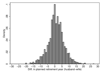
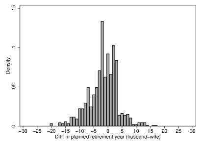
Notes: Figure 1 illustrates the difference in the year of retirement between husband and wife. The peak around zero indicates joint retirement planning. Because the SPA of women is lower from that of men for most cohorts, it is expected that the distribution is right-tailed. The left panel illustrates the unconditional distribution and the right panel illustrates the distribution conditional on the husband being at least 2 years older than his spouse.
Online supplemental material
Definition of Moments used for Estimation
Individual OLS Moment Conditions.
Let denote the planned retirement age of member in household and denote the set of control variables. We include as the first set of moments
where, for ,
where are the OLS regression coefficients using the data.
Covariance Matrix of Regression Residuals.
The second set of moments are related to the regression above. Particularly, we include as the second set of moments the simulated difference in the moments of the error terms
where is the residuals from the regression using the data.
Planned Retirement Age Groups.
Next, we include the share of individuals retiring in 6 particular age-groups, . Denote as the 6-element column vector of dummies where is one if member in household is in group and zero otherwise. Likewise, denote as the simulated counter-part of this set of dummies. We then include as the third set of moments,
Simultaneous retirement.
The final moments included relate to the retirement timing of couples. Defining the retirement calendar year as and the simulated counterpart as , the final moments are
Stacking all moments together gives
and the estimator of is
where we use as weighting a matrix, , the inverse of the bootstrapped variances of the moments on the diagonal and zero everywhere else.
We solve the minimization problem by successively applying different minimization routines in Matlab. We perform the sequence of estimators four times and report the estimates yielding the lowest criteria function. For each of the four estimation runs, we start with MATLABs particleswarm which is a “global” optimization routine using randomization to search through the parameter space. We use 80 particles and switch to Nelder-Mead (fminsearch in MATLAB) using the best candidates from the converged particleswarm. We use simulation draws for this estimation. After the four sequences of these two algorithms, we increase the number of simulation draws to and do one final Nelder-Mead minimization starting at the parameters yielding the lowest objective function over the four sequences of estimators. We then report the parameter values that solves this final minimization.