Minimally distorted Adversarial Examples with a Fast Adaptive Boundary Attack

Minimally distorted Adversarial Examples with a Fast Adaptive Boundary Attack

Abstract

The evaluation of robustness against adversarial manipulation of neural networks-based classifiers is mainly tested with empirical attacks as methods for the exact computation, even when available, do not scale to large networks. We propose in this paper a new white-box adversarial attack wrt the $l_{p}$-norms for $p\in\{1,2,\infty\}$ aiming at finding the minimal perturbation necessary to change the class of a given input. It has an intuitive geometric meaning, yields quickly high quality results, minimizes the size of the perturbation (so that it returns the robust accuracy at every threshold with a single run). It performs better or similar to state-of-the-art attacks which are partially specialized to one $l_{p}$-norm, and is robust to the phenomenon of gradient masking.

1 Introduction

The finding of the vulnerability of neural networks-based classifiers to adversarial examples, that is small perturbations of the input able to modify the decision of the models, started a fast development of a variety of attack algorithms. The high effectiveness of adversarial attacks reveals the fragility of these networks which questions their safe and reliable use in the real world, especially in safety critical applications. Many defenses have been proposed to fix this issue (Gu & Rigazio, 2015; Zheng et al., 2016; Papernot et al., 2016; Huang et al., 2016; Bastani et al., 2016; Madry et al., 2018), but with limited success, as new more powerful attacks showed (Carlini & Wagner, 2017b; Athalye et al., 2018; Mosbach et al., 2018). In order to trust the decision of a model, it is necessary to evaluate the exact adversarial robustness. Although this is possible for ReLU networks (Katz et al., 2017; Tjeng et al., 2019) these techniques do not scale to commonly used large networks. Thus, the robustness is evaluated approximating the solution of the minimal adversarial perturbation problem through adversarial attacks.
One can distinguish attacks into black-box (Narodytska & Kasiviswanathan, 2016; Brendel et al., 2018; Su et al., 2019), where one is only allowed to query the classifier, and white-box attacks, where one has full control over the network, according to the attack model used to create adversarial examples (typically some $l_{p}$-norm, but others have become popular as well, e.g. (Brown et al., 2017; Engstrom et al., 2017; Wong et al., 2019)), whether they aim at the minimal adversarial perturbation (Carlini & Wagner, 2017a; Chen et al., 2018; Croce et al., 2019) or rather any perturbation below a threshold (Kurakin et al., 2017; Madry et al., 2018; Zheng et al., 2019), if they have lower (Moosavi-Dezfooli et al., 2016; Modas et al., 2019) or higher (Carlini & Wagner, 2017a; Croce et al., 2019) computational cost. Moreover, it is clear that due to the non-convexity of the problem there exists no universally best attack (apart from the exact methods), since this depends on runtime constraints, networks architecture, dataset, etc. However, our goal is to have an attack which performs well under a broad spectrum of conditions with minimal amount of hyperparameter tuning.

In this paper we propose a new white-box attack scheme which performs comparably or better than established attacks and has the following features: first, it aims at adversarial samples with minimal distance to the attacked point, measured wrt the $l_{p}$-norms with $p\in\{1,2,\infty\}$. Compared to the popular PGD (projected gradient descent)-attack of (Madry et al., 2018) this has the clear advantage that our method does not need to be restarted for every threshold $\epsilon$ if one wants to evaluate the success rate of the attack with perturbations constrained to be in $\{\delta\in\mathbb{R}^{d}\,|\,\left\|\delta\right\|_{p}\leq\epsilon\}$. Thus it is particularly suitable to get a complete picture on the robustness of a classifier with low computational cost. Second, it achieves fast good quality in terms of average distortion or robust accuracy. At the same time we show that increasing the number of restarts keeps improving the results and makes it competitive to or stronger than the strongest available attacks. Third, although it comes with a few parameters, these generalize well across datasets, architectures and norms considered, so that we have an almost off-the-shelf method. Most importantly, unlike PGD and other methods, there is no step size parameter, which potentially has to be carefully adapted to every new network, and we show that it is scaling invariant. Both properties lead to the fact that it is robust to gradient masking which can be a problem for PGD (Tramèr & Boneh, 2019).

2 FAB: a Fast Adaptive Boundary Attack

We first introduce minimal adversarial perturbations, then we recall the definition and properties of the projection wrt the $l_{p}$-norms of a point on the intersection of a hyperplane and box constraints, as they are an essential part of our attack. Finally, we present our FAB-attack algorithm to generate minimally distorted adversarial examples.

2.1 Minimal adversarial examples

Let $f:\mathbb{R}^{d}\rightarrow\mathbb{R}^{K}$ be a classifier which assigns every input $x\in\mathbb{R}^{d}$ (with $d$ the dimension of the input space) to one of the $K$ classes according to $\mathop{\rm arg\,max}\limits_{r=1,\ldots,K}f_{r}(x)$. In many scenarios the input of $f$ has to satisfy a specific set of constraints $C$, e.g. images are represented as elements of $[0,1]^{d}$. Then, given a point $x\in\mathbb{R}^{d}$ with true class $c$, we define the minimal adversarial perturbation for $x$ wrt the $l_{p}$-norm as

$$\begin{split}&\delta_{\textrm{min},p}=\mathop{\rm arg\,min}\limits_{\delta\in\mathbb{R}^{d}}\;\left\|\delta\right\|_{p},\\ &\textrm{s.th.}\quad\mathop{\rm max}\limits_{l\neq c}\;f_{l}(x+\delta)\geq f_{c}(x+\delta),\quad x+\delta\in C.\end{split}$$ (1)

The optimization problem (LABEL:eq:advopt) is non-convex and NP-hard for non-trivial classifiers (Katz et al., 2017) and, although for some classes of networks it can be formulated as a mixed-integer program (Tjeng et al., 2019), the computational cost of solving it is prohibitive for large, normally trained networks. Thus, $\delta_{\textrm{min},p}$ is usually approximated by an attack algorithm, which can be seen as a heuristic to solve (LABEL:eq:advopt). We will see in the experiments that current attacks sometimes drastically overestimate $\left\|\delta_{\textrm{min},p}\right\|_{p}$ and thus the robustness of the networks.

2.2 Projection on a hyperplane with box constraints

Let $w\in\mathbb{R}^{d}$ and $b\in\mathbb{R}$ be the normal vector and the offset defining the hyperplane $\pi:\left\langle w,x\right\rangle+b=0$. Let $x\in\mathbb{R}^{d}$, we denote by the box-constrained projection wrt the $l_{p}$-norm of $x$ on $\pi$ (projection onto the intersection of the box $C=\{z\in\mathbb{R}^{d}:l_{i}\leq z_{i}\leq u_{i}\}$ and the hyperplane $\pi$) the following minimization problem:

$$z^{*}=\mathop{\rm arg\,min}\limits_{z\in\mathbb{R}^{d}}\;\left\|z-x\right\|_{p}$$ (2)

$$\textrm{s.th.}\quad\left\langle w,z\right\rangle+b=0,\quad l_{i}\leq z_{i}\leq u_{i},\;i=1,\ldots,d,$$

where $l_{i},u_{i}\in\mathbb{R}$ are lower and upper bounds on each component of $z$. For $p\geq 1$ the optimization problem (2) is convex. (Hein & Andriushchenko, 2017) proved that for $p\in\{1,2,\infty\}$ the solution can be obtained in $\mathcal{O}(d\log d)$ time, that is the complexity of sorting a vector of $d$ elements, as well as determining that there exists no feasible point.

Since this projection is part of our iterative scheme, we need to handle specifically the case of (2) being infeasible. In this case, defining $\rho=\mathop{\rm sign}\limits(\left\langle w,x\right\rangle+b)$, we instead compute $z^{\prime}=\mathop{\rm arg\,min}\limits_{l_{i}\leq z_{i}\leq u_{i}}\rho\cdot(\left\langle w,z\right\rangle+b)$, whose solution is

$$z_{i}^{\prime} =\begin{cases}l_{i}&\textrm{if }\rho w_{i}>0,\\ u_{i}&\textrm{if }\rho w_{i}<0,\\ x_{i}&\textrm{if }w_{i}=0\end{cases}\;\textrm{for}\;i=1,\ldots,d.$$ (3)

Assuming that the point $x$ satisfies the box constraints (as it holds in our algorithm), this is equivalent to identifying the corner of the $d$-dimensional box, defined by the componentwise constraints on $z$, closest to the hyperplane $\pi$. Note that if (2) is infeasible then the objective function of (3) stays positive and the points $x$ and $z$ are strictly contained in the same of the two halfspaces divided by $\pi$. Finally, we define the projection operator

$$\textrm{proj}_{p}:(x,\pi,C)\longmapsto\left\{\begin{array}[]{l l}z^{*}&\textrm{if }\eqref{eq:proj_1}\textrm{ is feasible}\\ z^{\prime}&\textrm{else}\end{array}\right.$$ (4)

which yields the point as close as possible to $\pi$ without violating the box constraints.

2.3 FAB-attack

We introduce now our algorithm to produce minimally distorted adversarial examples, wrt any $l_{p}$-norm for $p\in\{1,2,\infty\}$, for a given point $x_{\textrm{orig}}$ initially correctly classified by $f$ as class $c$. The high-level idea is that, first, we use the linearization of the classifier at the current iterate $x^{(i)}$ to compute the box-constrained projections of $x^{(i)}$ respectively $x_{\textrm{orig}}$ onto the approximated decision hyperplane and, second, we take a convex combinations of these projections depending on the distance of $x^{(i)}$ and $x_{\textrm{orig}}$ to the decision hyperplane. Finally, we perform an extrapolation step. We explain below the geometric motivation behind these steps. The attack closest in spirit is DeepFool (Moosavi-Dezfooli et al., 2016) which is known to be very fast but suffers from low quality. DeepFool just tries to find the decision boundary quickly but has no incentive to provide a solution close to $x_{\textrm{orig}}$. Our scheme resolves this main problem and, together with the exact projection we use, leads to a principled way to track the decision boundary (the surface where the decision of $f$ changes) close to $x_{\textrm{orig}}$.

If $f$ was a linear classifier then the closest point to $x^{(i)}$ on the decision hyperplane could be found in closed form. However neural networks are highly non-linear (although ReLU networks, i.e. neural networks which use ReLU as activation function, are piecewise affine functions and thus locally a linearization of the network is an exact description of the classifier). Let $l\neq c$, then the decision boundary between classes $l$ and $c$ can be locally approximated using a first order Taylor expansion at $x^{(i)}$ by the hyperplane

$$\begin{split}\pi_{l}(z):\;&f_{l}(x^{(i)})-f_{c}(x^{(i)})\\ &+\left\langle\nabla f_{l}(x^{(i)})-\nabla f_{c}(x^{(i)}),z-x^{(i)}\right\rangle=0.\end{split}$$ (5)

Moreover the $l_{p}$-distance $d_{p}(x^{(i)},\pi_{l})$ of $x^{(i)}$ to $\pi_{l}$ is given, assuming $\frac{1}{p}+\frac{1}{q}=1$, by

$$d_{p}(x^{(i)},\pi_{l})=\frac{|f_{l}(x^{(i)})-f_{c}(x^{(i)})|}{\left\|\nabla f_{l}(x^{(i)})-\nabla f_{c}(x^{(i)})\right\|_{q}}.$$ (6)

Note that if $d_{p}(x^{(i)},\pi_{l})=0$ then $x^{(i)}$ belongs to the true decision boundary. Moreover, if the local linear approximation of the network is correct then the class $s$ with the decision hyperplane closest to the point $x^{(i)}$ can be computed as

$$s=\mathop{\rm arg\,min}\limits_{l\neq c}\frac{|f_{l}(x^{(i)})-f_{c}(x^{(i)})|}{\left\|\nabla f_{l}(x^{(i)})-\nabla f_{c}(x^{(i)})\right\|_{q}}.$$ (7)

Thus, given that the approximation holds in some large enough neighborhood, the projection $\textrm{proj}_{p}(x^{(i)},\pi_{s},C)$ of $x^{(i)}$ onto $\pi_{s}$ lies on the decision boundary (unless (2) is infeasible).

Biased gradient step:

The iterative algorithm $x^{(i+1)}=\textrm{proj}_{p}(x^{(i)},\pi_{s},C)$ would be similar to DeepFool except that our projection operator is exact whereas they project onto the hyperplane and then clip to $[0,1]^{d}$. This scheme is not biased towards the original target point $x_{\textrm{orig}}$, thus it goes typically further than necessary to find a point on the decision boundary as basically the algorithm does not aim at the minimal adversarial perturbation. Then we consider additionally $\textrm{proj}_{p}(x_{\textrm{orig}},\pi_{s},C)$ and use instead the iterative step, with $x^{(0)}=x_{\textrm{orig}}$ and $\alpha\in[0,1]$, defined as

$$x^{(i+1)}=(1-\alpha)\,\textrm{proj}_{p}(x^{(i)},\pi_{s},C)+\alpha\,\textrm{proj}_{p}(x_{\textrm{orig}},\pi_{s},C),$$ (8)

which biases the step towards $x_{\textrm{orig}}$ (see Figure 1). Note that this is a convex combination of two points on $\pi_{s}$ and in $C$ and thus also $x^{(i+1)}$ lies on $\pi_{s}$ and is contained in $C$.

As we wish a scheme with minimal amount of parameters, our goal is an automatic selection of $\alpha$ based on the available geometric quantities. Let

$$\delta^{(i)}=\textrm{proj}_{p}(x^{(i)},\pi_{s},C)-x^{(i)},$$

$$\delta_{\textrm{orig}}^{(i)}=\textrm{proj}_{p}(x_{\textrm{orig}},\pi_{s},C)-x_{\textrm{orig}}.$$

Note that $\left\|\delta^{(i)}\right\|_{p}$ and $\left\|\delta^{(i)}_{\textrm{orig}}\right\|_{p}$ are the distances of $x^{(i)}$ and $x_{\textrm{orig}}$ to $\pi_{s}$ (inside $C$). We propose to use for the parameter $\alpha$ the relative magnitude of these two distances, that is

$$\alpha=\mathop{\rm min}\nolimits\left\{\frac{\left\|\delta^{(i)}\right\|_{p}}{\left\|\delta^{(i)}\right\|_{p}+\left\|\delta_{\textrm{orig}}^{(i)}\right\|_{p}},\alpha_{\textrm{max}}\right\}\in[0,1].$$ (9)

The motivation for doing so is that if $x^{(i)}$ is close to the decision boundary then we should stay close to this point (note that $\pi_{s}$ is the approximation of $f$ computed at $x^{(i)}$ and thus it is valid in a small neighborhood of $x^{(i)}$, whereas $x_{\textrm{orig}}$ is farther away). On the other hand we want to have the bias towards $x_{\textrm{orig}}$ in order not to go too far away from $x_{\textrm{orig}}$. This is why $\alpha$ depends on the distances of $x^{(i)}$ and $x_{\textrm{orig}}$ to $\pi_{s}$ but we limit it from above with $\alpha_{\mathop{\rm max}\nolimits}$. Finally, we use a small extrapolation step as we noted empirically, similarly to (Moosavi-Dezfooli et al., 2016), that this helps to cross faster the decision boundary and get an adversarial sample. This leads to the final scheme:

$$x^{(i+1)}=\textrm{proj}_{C}\Big{(}(1-\alpha)\big{(}x^{(i)}+\eta\delta^{(i)}\big{)}+\alpha\big{(}x_{\textrm{orig}}+\eta\delta^{(i)}_{\textrm{orig}}\big{)}\Big{)},$$ (10)

where $\alpha$ is chosen as in $\eqref{eq:alpha_step}$, $\eta\geq 1$ and $\textrm{proj}_{C}$ is the projection onto the box which can be done by clipping. In Figure 1 we visualize the scheme: in black one can see the hyperplane $\pi_{s}$ and the vectors $\delta_{\textrm{orig}}^{(i)}$ and $\delta^{(i)}$, in blue the step not biased towards $x_{\textrm{orig}}$, while in red the biased step of FAB-attack, see (10). The green vector shows the bias towards the original point we introduce. On the left of Figure 1 we use $\eta=1$, while on the right we use extrapolation $\eta>1$.

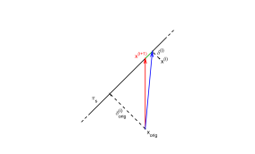
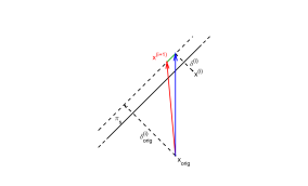
Figure 1: Visualization of FAB-attack scheme: Left, case $\eta=1$, right, $\eta>1$ (extrapolation). In blue we show $\textrm{proj}_{p}(x^{(i)},\pi_{s},C)$, the iterate one would get without any bias towards $x_{\textrm{orig}}$, in green the effect of the bias we introduce and in red the actual iterate $x^{(i+1)}$ of FAB-attack in (10). FAB-attack stays closer to $x_{\textrm{orig}}$ compared to the unbiased gradient step with $\textrm{proj}_{p}(x^{(i)},\pi_{s},C)$.

Interpretation of $\textrm{proj}_{p}(x_{\textrm{orig}},\pi_{s},C)$:

The projection of the target point $x_{\textrm{orig}}$ onto the intersection of $\pi_{s}$ and $C$ is

$$\mathop{\rm arg\,min}\limits_{z\in\mathbb{R}^{d}}\;\left\|z-x_{\textrm{orig}}\right\|_{p}\;\textrm{s.th.}\;\left\langle w,z\right\rangle+b=0,\;l_{i}\leq z_{i}\leq u_{i},$$

Note that replacing $z$ by $x^{(i)}+\delta$ we can rewrite this as

$$\begin{split}\mathop{\rm arg\,min}\limits_{\delta\in\mathbb{R}^{d}}\;&\left\|x^{(i)}+\delta-x_{\textrm{orig}}\right\|_{p}\\ \textrm{s.th.}\quad&\left\langle w,x^{(i)}+\delta\right\rangle+b=0,\quad l_{i}\leq x_{i}+\delta_{i}\leq u_{i}.\end{split}$$

This can be interpreted as the minimization of the distance of the next iterate $x^{(i)}+\delta$ to the target point $x_{\textrm{orig}}$ so that $x^{(i)}+\delta$ lies on the intersection of the (approximate) decision hyperplane and the box $C$. This point of view on the projection $\textrm{proj}_{p}(x_{\textrm{orig}},\pi_{s},C)$ again justifies using a convex combination of the two projections in our scheme in (10).

Backward step:

The described scheme finds in a few iterations adversarial perturbations. However, we are interested in minimizing their norms. Thus, once we have a new point $x^{(i+1)}$, we check whether it is assigned by $f$ to a class different from $c$. In this case, we apply

$$x^{(i+1)}=(1-\beta)x_{\textrm{orig}}+\beta x^{(i+1)},\quad\beta\in(0,1),$$ (11)

that is we go back towards $x_{\textrm{orig}}$ on the segment $[x^{(i+1)},x_{\textrm{orig}}]$, effectively starting again the algorithm at a point which is close to the decision boundary. In this way, due to the bias of the method towards $x_{\textrm{orig}}$ we successively find adversarial perturbations of smaller norm, meaning that the algorithm tracks the decision boundary while getting closer to $x_{\textrm{orig}}$. We fix $\beta=0.9$ in all experiments.

Final search:

Our scheme finds points close to the decision boundary but often they are slightly off as the linear approximation is not exact and we apply the extrapolation step with $\eta>1$. Thus, after finishing $N_{\textrm{iter}}$ iterations of our algorithmic scheme, we perform a last, fast step to further improve the quality of the adversarial examples. Let $x_{\textrm{out}}$ be the closest point to $x_{\textrm{orig}}$ classified differently from $c$, say $s\neq c$, found with the iterative scheme. It holds that $f_{s}(x_{\textrm{out}})-f_{c}(x_{\textrm{out}})>0$ and $f_{s}(x_{\textrm{orig}})-f_{c}(x_{\textrm{orig}})<0$. This means that, assuming $f$ continuous, there exists a point $x^{*}$ on the segment $[x_{\textrm{out}},x_{\textrm{orig}}]$ such that $f_{s}(x^{*})-f_{c}(x^{*})=0$ and $\left\|x^{*}-x_{\textrm{orig}}\right\|_{p}<\left\|x_{\textrm{out}}-x_{\textrm{orig}}\right\|_{p}$. If $f$ is linear

$$x^{*}=x_{\textrm{out}}-\frac{\left(f_{s}(x_{\textrm{out}})-f_{c}(x_{\textrm{out}})\right)(x_{\textrm{out}}-x_{\textrm{orig}})}{f_{s}(x_{\textrm{out}})-f_{c}(x_{\textrm{out}})+f_{s}(x_{\textrm{orig}})-f_{c}(x_{\textrm{orig}})}.$$ (12)

Since $f$ is non-linear, we compute iteratively for a few steps

$$x_{\textrm{temp}}=x_{\textrm{out}}-\frac{\left(f_{s}(x_{\textrm{out}})-f_{c}(x_{\textrm{out}})\right)(x_{\textrm{out}}-x_{\textrm{orig}})}{f_{s}(x_{\textrm{out}})-f_{c}(x_{\textrm{out}})+f_{s}(x_{\textrm{orig}})-f_{c}(x_{\textrm{orig}})},$$ (13)

each time replacing in (13) $x_{\textrm{out}}$ with $x_{\textrm{temp}}$ if $f_{s}(x_{\textrm{temp}})-f_{c}(x_{\textrm{temp}})>0$ or $x_{\textrm{orig}}$ with $x_{\textrm{temp}}$ if instead $f_{s}(x_{\textrm{temp}})-f_{c}(x_{\textrm{temp}})<0$. With this kind of modified binary search one can find a better adversarial sample with the cost of a few forward passes (which is fixed to $3$ in all experiments).

Random restarts:

So far all the steps are deterministic. To improve the results, we introduce the option of random restarts, that is $x^{(0)}$ is randomly sampled in the proximity of $x_{\textrm{orig}}$ instead of being $x_{\textrm{orig}}$ itself. Most attacks benefit from random restarts, e.g. (Madry et al., 2018; Zheng et al., 2019), especially dealing with models trained for robustness (Mosbach et al., 2018), as it allows a wider exploration of the input space. We choose to sample from the $l_{p}$-sphere centered in the original point with radius half the $l_{p}$-norm of the current best adversarial perturbation (or a given threshold if no adversarial example has been found yet).

Algorithm 1 FAB-attack

Input :

$x_{\textrm{orig}}$ original point, $c$ original class, $N_{\textrm{restarts}},N_{\textrm{iter}},\alpha_{\textrm{max}},\beta,\eta,\epsilon,p$

Output :

$x_{\textrm{out}}$ adversarial example

$u\leftarrow+\infty$
for $j=1,\ldots,N_{\textrm{restarts}}$ do

      if $j=1$ then $x^{(0)}\leftarrow x_{\textrm{orig}}$;

      else $x^{(0)}\leftarrow\textrm{randomly sampled s.th.}\left\|x^{(0)}-x_{\textrm{orig}}\right\|_{p}=\nicefrac{{\mathop{\rm min}\nolimits\{u,\epsilon\}}}{{2}}$;

      for $i=0,\ldots,N_{\textrm{iter}}-1$ do

          $s\leftarrow\mathop{\rm arg\,min}\limits_{l\neq c}\frac{|f_{l}(x^{(i)})-f_{c}(x^{(i)})|}{\left\|\nabla f_{l}(x^{(i)})-\nabla f_{c}(x^{(i)})\right\|_{q}}$
$\delta^{(i)}\leftarrow\textrm{proj}_{p}(x^{(i)},\pi_{s},C)$
$\delta^{(i)}_{\textrm{orig}}\leftarrow\textrm{proj}_{p}(x_{\textrm{orig}},\pi_{s},C)$
compute $\alpha$ as in Equation (9)
$\begin{aligned} x^{(i+1)}\leftarrow\textrm{proj}_{C}\Big{(}&(1-\alpha)\left(x^{(i)}+\eta\delta^{(i)}\right)\\ &+\alpha(x_{\textrm{orig}}+\eta\delta^{(i)}_{\textrm{orig}})\Big{)}\end{aligned}$
if $x^{(i+1)}$ is not classified as $c$ then

               if $\left\|x^{(i+1)}-x_{\textrm{orig}}\right\|_{p}<u$ then

                    $x_{\textrm{out}}\leftarrow x^{(i+1)}$
$u\leftarrow\left\|x^{(i+1)}-x_{\textrm{orig}}\right\|_{p}$

                     end if

                    $x^{(i+1)}\leftarrow(1-\beta)x_{\textrm{orig}}+\beta x^{(i+1)}$

                     end if

                    

                     end for

                    

                     end for

perform 3 steps of final search on $x_{\textrm{out}}$ as in (13)

Computational cost:

Our attack, in Algorithm 1, consists of two main operations: the computation of $f$ and its gradients and solving the projection (2). We perform, for each iteration, a forward and a backward pass of the network in the gradient step and a forward pass in the backward step. The projection can be efficiently implemented to run in batches on the GPU and its complexity depends only on the input dimension. Thus, except for shallow models, its cost is much smaller than the passes through the network. We can approximate the computational cost of our algorithm by the total number of calls of the classifier $N_{\textrm{iter}}\times N_{\textrm{restarts}}\times(2\times\textrm{forward passes}+1\times\textrm{backward pass})$ Per restart one has to add the three forward passes for the final search.

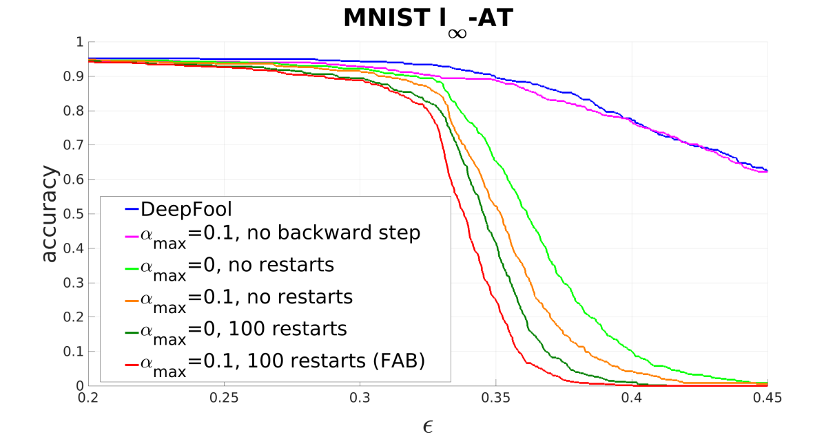
Figure 2: Ablation study to DeepFool for $l_{\infty}$-attacks. The curves show the robust accuracy as a function of the threshold $\epsilon$ under different attacks on the $l_{\infty}$-AT model on MNIST (lower values mean stronger attacks). The introduction of the convex combination ($\alpha_{\mathop{\rm max}\nolimits}=0.1$, no backward step) already improves over DeepFool. If one uses the backward step, the case $\alpha_{\mathop{\rm max}\nolimits}=0$ (which can be seen as an improved iterative DF) is worse than $\alpha_{\mathop{\rm max}\nolimits}=0.1$ with the same number of restarts.

2.4 Scale Invariance of FAB-attack

For a given classifier $f$, the decisions and thus adversarial samples do not change if we rescale the classifier $g=\alpha f$ for $\alpha>0$ or shift its logits as $h=f+\beta$ for $\beta\in\mathbb{R}$. The following proposition states that FAB-attack is invariant under both rescaling and shifting (proof in Section A).

Proposition 2.1

Let $f:\mathbb{R}^{d}\rightarrow\mathbb{R}^{K}$ be a classifier. Then for any $\alpha>0$ and $\beta\in\mathbb{R}$ the output $x_{\textrm{out}}$ of Algorithm 1 for the classifier $f$ is the same as of the classifiers $g=\alpha f$ and $h=f+\beta$.

We note that the cross-entropy loss $\textrm{CE}(x,y,f)=-\log(e^{f_{y}(x)}/\sum_{j=1}^{K}e^{f_{j}(x)})$ used as objective in the normal PGD attack and its gradient wrt $x$

$$\nabla_{x}\textrm{CE}(x,y,f)=-\nabla_{x}f_{y}(x)+\frac{\sum_{j=1}^{K}e^{f_{j}(x)}\nabla_{x}f_{j}(x)}{\sum_{j=1}^{K}e^{f_{j}(x)}}$$

are not invariant under rescaling. Moreover, we observe that the gradient vanishes for $\alpha f$ if $f_{y}(x)>f_{j}(x)$ for $j\neq y$ (correctly classified point) as $\alpha\rightarrow\infty$. Due to finite precision the gradient becomes zero for finite $\alpha$ and it is obvious that in this case PGD gets stuck. Due to the rescaling invariance FAB-attack is not affected by gradient masking due to this phenomenon as it uses the gradient of the differences of the logits and not the gradient of the cross-entropy loss. The latter one runs much earlier into numerical problems when one upscales the classifier due to the exponential function. In the experiments (see below) we show that PGD can catastrophically fail due to a “wrong” scaling whereas FAB-attack is unaffected.

2.5 Comparison to DeepFool

The idea of exploiting the first order local approximation of the decision boundary is not novel but the basis of one of the first white-box adversarial attacks, DeepFool (DF) from (Moosavi-Dezfooli et al., 2016). While DF and our FAB-attack share the strategy of using a linear approximation of the classifier and projecting on the decision hyperplanes, we want to point out many key differences: first, DF does not solve the projection (2) but its simpler version without box constraints, clipping afterwards. Second, their gradient step does not have any bias towards the original point, that is equivalent to $\alpha=0$ in (10). Third, DF does not have any backward step, final search or restart, as it stops as soon as a misclassified point is found (its goal is to provide quickly an adversarial perturbation of average quality).
We perform an ablation study of the differences to DF in Figure 2, where we show robust accuracy as a function of the threshold $\epsilon$ (lower is better). We present the results of DeepFool (blue) and FAB-attack with the following variations: $\alpha_{\textrm{max}}=0.1$ and no backward step (magenta), $\alpha_{\textrm{max}}=0$ (that is no bias in the gradient step) and no restarts (light green), $\alpha_{\textrm{max}}=0.1$ and no restarts (orange), $\alpha_{\textrm{max}}=0$ and 100 restarts (dark green) and $\alpha_{\textrm{max}}=0.1$ and 100 restarts, that is FAB-attack, (red). We can see how every addition we make to the original scheme of DeepFool contributes to the significantly improved performance of FAB-attack when compared to the original DeepFool.

3 Experiments

Models:

We run experiments on MNIST, CIFAR-10 (Krizhevsky et al., 2014) and Restricted ImageNet (Tsipras et al., 2019). For each dataset we consider a normally trained model (plain) and two adversarially trained ones as in (Madry et al., 2018) wrt the $l_{\infty}$-norm ($l_{\infty}$-AT) and the $l_{2}$-norm ($l_{2}$-AT) (see B.1 for details).

MNIST - $l_{\infty}$-attack:

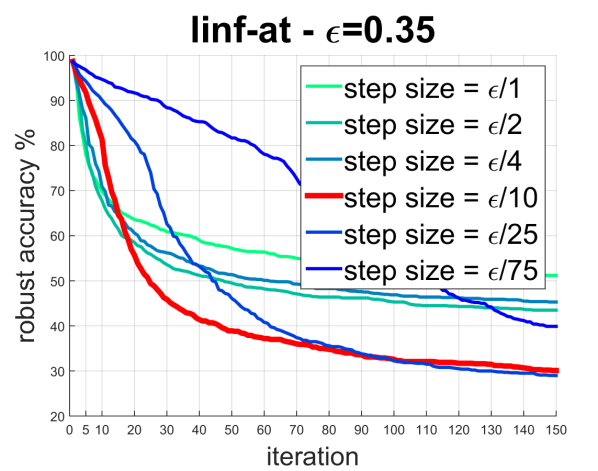
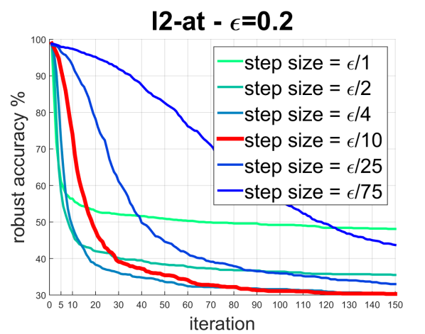
MNIST - $l_{2}$-attack:

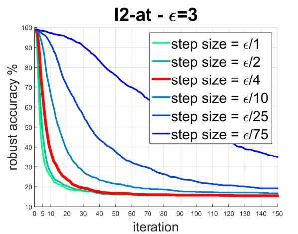
MNIST - $l_{1}$-attack:

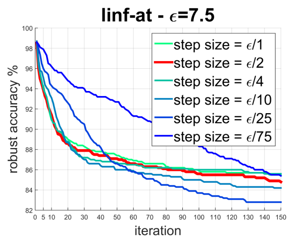
Figure 3: Evolution of robust accuracy across iterations for different step sizes for PGD wrt $l_{1},l_{2},l_{\infty}$ for three different models on MNIST. In red we highlight the step size we used for each norm in the experiments. Notice that it performs on average the best. Here we evaluate on MNIST - the supplementary material contains also CIFAR-10 and other thresholds.

Table 1: Performance summary of all attacks on MNIST and CIFAR-10 (aggregated). We report, for each norm, "avg. rob. acc.", the mean of robust accuracies across all models and datasets (lower is better), "# best", number of times the attack is the best one, "avg. diff. to best" and "max diff. to best", the mean and maximum difference of the robust accuracy of the attack to the robust accuracy of the best attack for each model/threshold (on the first 1000 points for $l_{\infty}$ and $l_{1}$, 500 for $l_{2}$, of the test sets). The numbers after the name of the attacks indicate the number of restarts. In total we have 5 thresholds $\times$ 6 models = 30 cases for each of the 3 norms. *Note that for FAB-10 (i.e. with 10 restarts) the "# best" is computed excluding the results of FAB-100.

statistics on MNIST + CIFAR-10
$l_{\infty}$-norm		DF	DAA-50	PGD-100	FAB-10	FAB-100
avg. rob. acc.		58.81	60.67	46.07	46.18	45.47
# best		0	8	12	13*	17
avg. diff. to best		14.58	16.45	1.85	1.96	1.25
max diff. to best		78.10	49.00	10.70	20.30	17.10
$l_{2}$-norm	CW	DF	LRA	PGD-100	FAB-10	FAB-100
avg. rob. acc.	45.09	56.10	36.97	44.94	36.41	35.57
# best	4	1	9	11	19*	23
avg. diff. to best	9.65	20.67	1.54	9.51	0.98	0.13
max diff. to best	65.40	91.40	13.60	64.80	8.40	1.60
$l_{1}$-norm		SF	EAD	PGD-100	FAB-10	FAB-100
avg. rob. acc.		64.47	35.79	49.51	33.26	29.46
# best		0	13	0	10*	17
avg. diff. to best		35.31	6.63	20.35	4.10	0.30
max diff. to best		95.90	58.40	74.00	21.80	1.60

Table 2: As in Table 1 statistics of the performance of different attacks on Restricted ImageNet (on the first 500 points of the validation set). In total we consider 5 thresholds $\times$ 3 models = 15 cases for each of the 3 norms.

statistics on Restricted ImageNet
	$l_{\infty}$-norm				$l_{2}$-norm			$l_{1}$-norm
	DF	DAA-10	PGD-10	FAB-10	DF	PGD-10	FAB-10	SF	PGD-5	FAB-5
avg. rob. acc.	35.61	38.44	26.91	27.83	45.69	31.75	33.24	71.31	40.64	38.12
# best	0	1	13	3	0	14	1	0	3	12
avg. diff. best	8.75	11.57	0.04	0.96	13.99	0.04	1.53	33.52	2.85	0.33
max diff. best	14.60	37.20	0.40	2.00	25.40	0.60	3.40	59.00	6.20	2.40

Attacks:

We compare the performance of FAB-attack to those of attacks representing the state-of-the-art in each norm: DeepFool (DF) (Moosavi-Dezfooli et al., 2016), Carlini-Wagner $l_{2}$-attack (CW) (Carlini & Wagner, 2017a), Linear Region $l_{2}$-Attack (LRA) (Croce et al., 2019), Projected Gradient Descent on the cross-entropy function (PGD) (Kurakin et al., 2017; Madry et al., 2018; Tramèr & Boneh, 2019), Distributionally Adversarial Attack (DAA) (Zheng et al., 2019), SparseFool (SF) (Modas et al., 2019), Elastic-net Attack (EAD) (Chen et al., 2018). We use DF from (Rauber et al., 2017), CW and EAD as in (Papernot et al., 2017), DAA and LRA with the code from the original papers, while we reimplemented SF and PGD. For MNIST and CIFAR-10 we used DAA with 50 restarts, PGD and FAB with 100 restarts. For Restricted ImageNet, we used DAA, PGD and FAB with 10 restarts (for $l_{1}$ we used 5 restarts, since the methods benefit from more iterations). Moreover, we could not use LRA since it hardly scales to models of such scale and CW and EAD for compatibility issues between the implementations of attacks and models. See B.2 for more details e.g. regarding number of iterations and hyperparameters of all attacks. In particular, we provide in Section C.1 a detailed analysis of the dependency of PGD on the step size. Indeed the optimal choice of the step size is quite important for PGD. In order to select the optimal step size for PGD for each norm, we performed a grid search on the step size parameter in $\nicefrac{{\epsilon}}{{t}}$ for $t\in\{1,2,4,10,25,75\}$ for different models and thresholds, and took the values working best on average, see Figure 3 for an illustration (similar plots for other datasets and thresholds are presented in Section C.1). As a result we use for PGD wrt $l_{\infty}$ step size $\nicefrac{{\epsilon}}{{10}}$ and the direction is the sign of the gradient of the cross entropy loss, for PGD wrt $l_{2}$ we do a step in the direction of the $l_{2}$-normalized gradient with step size $\nicefrac{{\epsilon}}{{4}}$, for PGD wrt $l_{1}$ we use the gradient step suggested in (Tramèr & Boneh, 2019) (with sparsity levels of 1% for MNIST and 10% for CIFAR-10 and Restricted ImageNet) with step size $\nicefrac{{\epsilon}}{{2}}$. For FAB-attack we use always $\beta=0.9$ and on MNIST and CIFAR-10: $\alpha_{\textrm{max}}=0.1$, $\eta=1.05$ and on Restricted ImageNet: $\alpha_{\mathop{\rm max}\nolimits}=0.05$, $\eta=1.3$. These parameters are the same for all norms.

Evaluation metrics:

The robust accuracy for a threshold $\epsilon$ is the classification accuracy (in percentage) when an adversary is allowed to change every test input with perturbations of $l_{p}$-norm smaller than $\epsilon$ in order to change the decision. Thus stronger attacks produce lower robust accuracies. For each model and dataset we fix five thresholds at which we compute the robust accuracy for each attack (we choose the thresholds so that the robust accuracy covers the range between clean accuracy and 0). We evaluate the attacks by the following statistics: i) avg. rob. accuracy: the mean of the robust accuracies achieved by the attack over all models and thresholds (lower is better), ii) # best: how many times the attack achieves the lowest robust accuracy (it is the most effective), iii) avg. difference to best: for each model/threshold we compute the difference between the robust accuracy of the attack and the best one across all the attacks, then we average over all models/thresholds, iv) max difference to best: as "avg. difference to best", but with the maximum difference instead of the average one. In Section B.4 we report additionally the average $l_{p}$-norm of the adversarial perturbations given by the attacks.

Results:

We report the complete results in Tables 7 to 15 of the appendix, while we summarize them in Table 1 (MNIST and CIFAR-10 aggregated, as we used the same attacks) and Table 2 (Restricted ImageNet). Our FAB-attack achieves the best results in all statistics for every norm (with the only exception of "max diff. to best" in $l_{\infty}$) on MNIST+CIFAR-10. In particular, while on $l_{\infty}$ the "avg. robust accuracy" of PGD is not far from that of FAB, the gap is large when considering $l_{2}$ and $l_{1}$ (in the appendix we provide in Table 5 the aggregate statistics without the result on $l_{\infty}$-AT MNIST, showing that FAB is still the best attack even if one leaves out this failure case of PGD). Interestingly, the second best attack in terms of average robust accuracy, is different for every norm (PGD for $l_{\infty}$, LRA for $l_{2}$, EAD for $l_{1}$), which implies that FAB outperforms algorithms specialized in the individual norms.
We also report the results of FAB-10, that is our attack with only 10 restarts, to show that FAB yields high quality results already with a low budget in terms of time/computational cost. In fact, FAB-10 has "avg. robust accuracy" better than or very close to that of the strongest versions of the other attacks (see below for a runtime analysis, where one observes that FAB-10 is the fastest attack when excluding the significantly worse DF and SF attacks). On Restricted ImageNet, FAB-attack gets the best results in all statistics for $l_{1}$, while for $l_{\infty}$ and $l_{2}$ PGD performs on average better, but the difference in "avg. robust accuracy" is small.
In general, both average and maximum difference to best of FAB-attack are small for all the datasets and norms, implying that it does not suffer from severe failures, which makes it an efficient, high quality technique to evaluate the robustness of classifiers for all $l_{p}$-norms. Finally, we show in Table 6 that FAB-attack outperforms or matches the competitors in 16 out of 18 cases when comparing the average $l_{p}$-norms of the generated adversarial perturbations.

Table 3: We attack the ResNet-110 in (Pang et al., 2020) on CIFAR-10 at $\epsilon=\nicefrac{{8}}{{255}}$. The performance of the PGD attack on the cross entropy loss (CE) heavily depends on both scale of the classifier and the step size. In contrast, the scaling invariant FAB-attack works well even on the original (unscaled) model.

attack	step size	robust accuracy
PGD-CE	$\nicefrac{{\epsilon}}{{10}}$	90.2%
PGD-CE	$\nicefrac{{\epsilon}}{{2}}$	90.2%
PGD-CE rescaled	$\nicefrac{{\epsilon}}{{10}}$	12.9%
PGD-CE rescaled	$\nicefrac{{\epsilon}}{{2}}$	2.5%
FAB	-	0.3%

Resistance to gradient masking:

It has been argued (Tramèr & Boneh, 2019) that models trained with first-order methods to be resistant wrt $l_{\infty}$-attacks on MNIST (adv. training) give a false sense of robustness in $l_{1}$ and $l_{2}$ due to gradient masking. This means that standard gradient-based methods like PGD have problems to find adversarial examples while they still exist. In contrast, FAB does not suffer from gradient masking. In Table 8 of the appendixwe see that it is extremely effective also wrt $l_{1}$ and $l_{2}$ on the $l_{\infty}$-robust model, outperforming by a large margin the competitors. The reason is that FAB is not dependent on the norm of the gradient but just its direction matters for the definition of the hyperplane in (5). While we believe that resistance to gradient masking is a key property of a solid attack, we recompute the statistics of Table 1 excluding $l_{1}$ and $l_{2}$ attacks on the $l_{\infty}$-AT model on MNIST in Table 5 in the appendix. FAB still achieves in most of the cases the best aggregated statistics, implying that our attack is effective whether or not the attacked classifier tends to "mask" the gradient.
We have shown in Section 2.4 that FAB-attack is invariant under rescaling of the classifier. We provide an example why this is a desirable property of an adversarial attack. We consider the defense proposed in (Pang et al., 2020), in particular their ResNet-110 (without adversarial training) for CIFAR-10. In Table 5 in (Pang et al., 2020) it is claimed that this model has a robust accuracy of 31.4% for $\nicefrac{{8}}{{255}}$ obtained by a PGD attack on their new loss function. They say that a standard PGD attack on the cross-entropy loss performs much worse. We test the performance of PGD on the cross-entropy loss, both using the original classifier and the same scaled down by a factor of $10^{6}$. Moreover, we use the default step size $\nicefrac{{\epsilon}}{{10}}$ together with $\nicefrac{{\epsilon}}{{2}}$. The results are reported in Table 3. We can see that PGD on the original model yields more than 90% robust accuracy which confirms the statement in (Pang et al., 2020) about the cross-entropy loss being unsuitable for this case. However, PGD applied to the rescaled classifier reduces robust accuracy below 13%. The better step size $\nicefrac{{\epsilon}}{{2}}$ decreases it to 2.5% which shows that tuning the stepsize is important for PGD. At the same time, FAB achieves a robust accuracy of 0.3% without any need of parameter tuning or rescaling of the classifier. This exemplifies the benefit of the scaling invariance of FAB. Moreover, as a side result this shows that the new loss alone in (Pang et al., 2020) is an ineffective defense.

Runtime comparison:

DF and SF are much faster than the other attacks as their primary goal is to find as fast as possible adversarial examples, without emphasis on minimizing their norms, while LRA is rather expensive as noted in the original paper. PGD needs a forward and a backward pass of the network per iteration whereas FAB requires three passes for each iteration. Thus PGD is given 1.5 times more iterations than FAB, so that overall they have same budget of forward/backward passes (and thus runtime). Below we report the runtimes (for 1000 points on MNIST and CIFAR-10, 50 on R-ImageNet) for the attacks as used in the experiments (if not specified otherwise, it includes all the restarts). For PGD and DAA this is the time for evaluating the robust accuracy at 5 thresholds, while for the other methods a single run is sufficient to compute the robust accuracy for all five thresholds. MNIST: DAA 11736s, PGD 3825s for $l_{\infty}$/$l_{2}$ and 14106s for $l_{1}$, CW 944s, EAD 606s, FAB-10 161s, FAB-100 1613s. CIFAR-10: DAA 11625s, PGD 31900s for $l_{\infty}$/$l_{2}$ and 70110s for $l_{1}$, CW 3691s, EAD 3398s, FAB-10 1209s, FAB-100 12093s. R-ImageNet: DAA 6890s, PGD 4738s for $l_{\infty}$/$l_{2}$ and 24158s for $l_{1}$, FAB 2268s for $l_{\infty}$/$l_{2}$ and 3146s for $l_{1}$ (note that for $l_{1}$ different numbers of restarts/iterations are used on R-ImageNet).
We note that for PGD the robust accuracy for the five thresholds can be computed faster by exploiting the fact that points which are non-robust for a thresholds $\epsilon$ are also non-robust for thresholds larger than $\epsilon$. However, even when taking this into account FAB-10 would still be significantly faster than PGD-100 and has better quality on MNIST and CIFAR-10. Moreover, when just considering a fixed number of thresholds, one can stop FAB-attack whenever it finds an adversarial example for the smallest threshold which also leads to a speed-up. However, in real world applications a full picture of robustness as a continuous function of the threshold is the most interesting evaluation scenario.

3.1 Additional results

In Section C.2 we show how the robust accuracy provided by either PGD or FAB-attack evolves over iterations, when only one start it used. In particular, we compare the two methods when the same number of passes, forward or backward, of the networks are used. One can observe that a few steps are usually sufficient for FAB-attack to achieve good results, often faster than PGD, although there are cases where a higher number of iterations leads to significantly better robust accuracy.

Finally, (Croce & Hein, 2020) use FAB-attack together with other white- and black-box attacks to evaluate the robustness of over 50 classifiers trained with recently proposed adversarial defenses wrt $l_{\infty}$ and $l_{2}$ on different datasets. With fixed hyperparameters, FAB-attack yields the best results in most of the cases on CIFAR-10, CIFAR-100 and ImageNet in both norms, in particular compared to different variations of PGD (with and without a momentum term, with different step sizes and using various losses). This shows again that FAB-attack is very effective for testing the robustness of adversarial defenses.

4 FAB-attack with a large number of classes

The standard algorithm of FAB-attack requires to compute at each iteration the Jacobian matrix of the classifier $f$ wrt the input $x$ and then the closest approximated decision hyperplane. The Jacobian matrix has dimension $K\times d$, recalling that $K$ is the number of classes and $d$ the input dimension. Although this can be in principle obtained with a single backward pass of the network, it becomes computationally expensive on datasets with many classes. Moreover, the memory consumption of FAB-attack increases with $K$. As a consequence, using FAB-attack in the normal formulation on datasets like ImageNet which has $K=1000$ classes may be inefficient.

Then, we propose a targeted version of our attack which performs at each iteration the projection onto the linearized decision boundary between the original class and a fixed target class. This means that in (8) the hyperplane $\pi_{s}$ is not selected via (7) as the closest one to the current iterate but rather $s\equiv t$, with $t$ the target class used. Note that in practice we do not constrain the final outcome of the algorithm to be assigned to class $t$, but any misclassification is sufficient to have a valid adversarial example. The target class $t$ is selected as the second most likely one according to the score given by the model to the target point, and if $k$ restarts are allowed one can use the classes with the $k+1$ highest scores as target (excluding the correct one $c$). In this way, only the gradient of $f_{t}-f_{c}:\mathbb{R}^{d}\rightarrow\mathbb{R}$ needs to be computed, which is a cheaper operation than getting the full Jacobian of $f$ and with computational cost independent of the total number of classes.

This targeted version of FAB-attack has been used in (Croce & Hein, 2020) considering the top-10 classes where it yields on CIFAR-10, CIFAR-100 and ImageNet almost always better robust accuracy than normal FAB-attack, which instead is almost always better on MNIST.

5 Conclusion

In summary, our geometrically motivated FAB-attack outperforms in terms of average quality the state-of-the-art attacks, already with a limited computational effort, and works for all $l_{p}$-norms in $p\in\{1,2,\infty\}$ unlike most competitors. Thanks to its scaling invariance and being step size free it is resistant to gradient masking and thus more reliable for assessing robustness than the standard PGD attack.

Appendix A Scale invariance of FAB-attack

We here describe the proof of Proposition 2.1.

Proposition 2.1

Let $f:\mathbb{R}^{d}\rightarrow\mathbb{R}^{K}$ be a classifier. Then for any $\alpha>0$ and $\beta\in\mathbb{R}$ the output $x_{\textrm{out}}$ of Algorithm 1 for the classifier $f$ is the same as of the classifiers $g=\alpha f$ and $h=f+\beta$.

Proof. It holds $\nabla g_{i}=\nabla\alpha f_{i}=\alpha\nabla f_{i}$ and $\nabla h_{i}=\nabla(f_{i}+\beta)=\nabla f_{i}$ for $i=1,\ldots,K$ and thus the definition of the hyperplane $\pi_{l}(z)$ in (5) is not affected by rescaling or shifting. The same holds for the distance of $x^{(i)}$ to the hyperplane $\pi_{l}(z)$ in (7). Note that the rest of the steps just depends on geometric quantities derived from these quantities and are independent of $f$. Finally, also the iterates of the final search in (13) are invariant under rescaling and shifting and thus the output $x_{\textrm{out}}$ of Algorithm 1 is invariant under rescaling of $f$. $\square$

Appendix B Experiments

B.1 Models

The plain and $l_{\infty}$-AT models on MNIST are those available at https://github.com/MadryLab/mnist_challenge and consist of two convolutional and two fully-connected layers. The architecture of the CIFAR-10 models has 8 convolutional layers (with number of filters increasing from 96 to 384) and 2 dense layers and we make the classifiers available at https://github.com/fra31/fab-attack, while on Restricted ImageNet we use the models (ResNet-50 (He et al., 2016)) from (Tsipras et al., 2019) and available at https://github.com/MadryLab/robust-features-code.
The models on MNIST achieve the following clean accuracy: plain 98.7%, $l_{\infty}$-AT 98.5%, $l_{2}$-AT 98.6%. The models on CIFAR-10 achieve the following clean accuracy: plain 89.2%, $l_{\infty}$-AT 79.4%, $l_{2}$-AT 81.2%.

B.2 Attacks

We use CW with 40 binary search steps, 10000 iterations and confidence 0, EAD with 1000 iterations, $l_{1}$ decision rule and $\beta=0.05$. In both cases we set the parameters to achieve minimally (wrt $l_{2}$ for CW and $l_{1}$ for EAD) distorted adversarial examples. We could not use these methods on Restricted ImageNet since, to be compatible with the attacks from (Papernot et al., 2017), it would be necessary to reimplement from scratch the models of (Tsipras et al., 2019), as done in https://github.com/tensorflow/cleverhans/tree/master/cleverhans/model_zoo/madry_lab_challenges for a similar situation.

For DAA we use 200 iterations for MNIST, 50 for the other datasets and, given a threshold $\epsilon$, a step size of $\nicefrac{{\epsilon}}{{30}}$ for MNIST, $\nicefrac{{\epsilon}}{{10}}$ otherwise.

We apply PGD with 150 iterations, except for the case of $l_{1}$ on Restricted ImageNet where we use 450 iterations. To choose the step size for each norm, we performed a grid search on the step size in $\nicefrac{{\epsilon}}{{t}}$ for $t\in\{1,2,4,10,25,75\}$ for different models and took the values working best on average (note that this gives an advantage to PGD). A more detailed analysis of the dependency of PGD on the step size is given in Section C.1. As a result we use for PGD wrt $l_{\infty}$ a step size of $\nicefrac{{\epsilon}}{{10}}$ and the direction is the sign of the gradient of the cross-entropy loss, for PGD wrt $l_{2}$ we do a step in the direction of the normalized gradient of size $\nicefrac{{\epsilon}}{{4}}$, for PGD wrt $l_{1}$ we use the gradient step suggested in (Tramèr & Boneh, 2019) (with sparsity levels of 1% for MNIST and 10% for CIFAR-10 and Restricted ImageNet) with step size $\nicefrac{{\epsilon}}{{2}}$.

For FAB-attack we set 100 iterations, except for the case of $l_{1}$ on Restricted ImageNet where we use 300 iterations. Moreover, we use the following parameters for all the cases on MNIST and CIFAR-10: $\alpha_{\textrm{max}}=0.1$, $\eta=1.05$, $\beta=0.9$. On Restricted ImageNet we set $\alpha_{\mathop{\rm max}\nolimits}=0.05$, $\eta=1.3$, $\beta=0.9$. When using random restarts, FAB-attack needs a value for the parameters $\epsilon$. It represents the radius of the $l_{p}$-ball around the original point inside which we sample the starting point of the algorithm, at least until a sufficiently small adversarial perturbation is found (see Algorithm 1). We use the values of $\epsilon$ reported in Table 4. Note that the attack usually finds at the first run an adversarial perturbation small enough so that $\epsilon$ in practice rarely comes into play.

Table 4: We report the values of $\epsilon$ used for sampling in case our FAB-attack uses random restarts.

values of $\epsilon$ used for random restarts
	MNIST			CIFAR-10			Restricted ImageNet
	plain	$l_{\infty}$-AT	$l_{2}$-AT	plain	$l_{\infty}$-AT	$l_{2}$-AT	plain	$l_{\infty}$-AT	$l_{2}$-AT
$l_{\infty}$	0.15	0.3	0.3	0.0	0.02	0.02	0.02	0.08	0.08
$l_{2}$	2.0	2.0	2.0	0.5	4.0	4.0	5.0	5.0	5.0
$l_{1}$	40.0	40.0	40.0	10.0	10.0	10.0	100.0	250.0	250.0

B.3 Complete results

In Tables 7 to 15 we report the complete values of the robust accuracy, wrt either $l_{\infty}$, $l_{2}$ or $l_{1}$, computed by every attack, for 3 datasets, 3 models for each dataset, 5 thresholds for each model (135 evaluations overall). In Table 5 we provide the aggreate statistics on MNIST and CIFAR-10 without the $l_{\infty}$-AT model of Madry, as there PGD fails completely for $l_{1}$- and $l_{2}$-attacks. FAB has still the better aggregate statistics if one leaves out these cases.

Table 5: Performance summary of all attacks on MNIST and CIFAR-10 (aggregated). We report, for each norm, "avg. rob. acc.", the mean of the robust accuracies across all models and datasets (lower is better), "# best", number of times the attack is the best one, "avg. diff. to best" and "max diff. to best", the mean and maximum difference of the robust accuracy of the attack to the robust accuracy of the best attack for each model/threshold (on the first 1000 points for $l_{\infty}$ and $l_{1}$, 500 for $l_{2}$, of the test sets). The numbers after the name of the attacks indicate the number of restarts. In total we have 5 thresholds $\times$ 6 models = 30 cases for each of the 3 norms. *Note that for FAB-10 (i.e. with 10 restarts) the "# best" is computed excluding the results of FAB-100. We also recompute the statistics excluding the $l_{\infty}$-AT model on MNIST from (Madry et al., 2018) where PGD fails in order to show that even excluding this case FAB is still the best.

statistics on MNIST + CIFAR-10
$l_{\infty}$-norm		DF	DAA-50	PGD-100	FAB-10	FAB-100
avg. rob. acc.		58.81	60.67	46.07	46.18	45.47
# best		0	8	12	13*	17
avg. diff. to best		14.58	16.45	1.85	1.96	1.25
max diff. to best		78.10	49.00	10.70	20.30	17.10
$l_{2}$-norm	CW	DF	LRA	PGD-100	FAB-10	FAB-100
avg. rob. acc.	45.09	56.10	36.97	44.94	36.41	35.57
# best	4	1	9	11	19*	23
avg. diff. to best	9.65	20.67	1.54	9.51	0.98	0.13
max diff. to best	65.40	91.40	13.60	64.80	8.40	1.60
$l_{2}$-norm wo/ $l_{\infty}$-AT model on MNIST	CW	DF	LRA	PGD-100	FAB-10	FAB-100
avg. rob. acc.	40.85	49.18	40.25	42.95	39.98	39.57
# best	4	1	8	11	14*	18
avg. diff. to best	1.44	9.78	0.84	3.54	0.57	0.16
max diff. to best	8.80	44.00	4.00	22.00	4.20	1.60
$l_{1}$-norm		SF	EAD	PGD-100	FAB-10	FAB-100
avg. rob. acc.		64.47	35.79	49.51	33.26	29.46
# best		0	13	0	10*	17
avg. diff. to best		35.31	6.63	20.35	4.10	0.30
max diff. to best		95.90	58.40	74.00	21.80	1.60
$l_{1}$-norm wo/ $l_{\infty}$-AT model on MNIST		SF	EAD	PGD-100	FAB-10	FAB-100
avg. rob. acc.		58.06	32.56	43.82	33.79	32.06
# best		0	13	0	5*	12
avg. diff. to best		26.36	0.87	12.12	2.10	0.36
max diff. to best		53.10	4.80	31.90	3.90	1.60

B.4 Further results

In Table 6 we report the average $l_{p}$-norm of the adversarial perturbations found by the different attacks, computed on the originally correctly classified points on which the attack is successful. Note that we cannot show this statistic for the attacks which do not minimize the distance of the adversarial example to the clean input (PGD and DAA). FAB-attack produces also in this metric the best results in most of the cases, being the best for every model when considering $l_{\infty}$ and $l_{2}$, and the best in 4 out of 6 cases in $l_{1}$ (lower values mean a stronger attack).

Table 6: We report mean $l_{p}$-norm of the adversarial perturbations found by the attacks (when successful, excluding the already misclassified points) for every model.

average norm of adversarial perturbations
$l_{\infty}$-norm				DF	FAB
MNIST	plain			0.078	0.066
	$l_{\infty}$-at			0.508	0.326
	$l_{2}$-at			0.249	0.170
CIFAR-10	plain			0.008	0.006
	$l_{\infty}$-at			0.032	0.024
	$l_{2}$-at			0.026	0.019
$l_{2}$-norm		DF	CW	LRA	FAB
MNIST	plain	1.13	1.01	1.00	1.00
	$l_{\infty}$-at	4.95	1.76	1.25	1.12
	$l_{2}$-at	3.10	2.35	2.25	2.24
CIFAR-10	plain	0.28	0.21	0.22	0.21
	$l_{\infty}$-at	0.96	0.74	0.74	0.73
	$l_{2}$-at	0.91	0.71	0.72	0.70
$l_{1}$-norm				EAD	FAB
MNIST	plain			6.38	6.04
	$l_{\infty}$-at			8.26	3.36
	$l_{2}$-at			12.18	12.16
CIFAR-10	plain			3.01	2.87
	$l_{\infty}$-at			5.79	6.03
	$l_{2}$-at			7.94	8.05

Table 7: Comparison of $l_{\infty}$-, $l_{2}$- and $l_{1}$-attacks on a naturally trained model on MNIST. We report the accuracy in percentage of the classifier on the test set if the attack is allowed to perturb the test points of $\epsilon$ in $l_{p}$-distance. The statistics are computed on the first 1000 points on the test set for $l_{\infty}$ and $l_{1}$, on 500 points for $l_{2}$.

Robust accuracy of MNIST plain model
metric	$\epsilon$	DF	DAA-1	DAA-50	PGD-1	PGD-10	PGD-100	FAB-1	FAB-10	FAB-100
$l_{\infty}$	0.03	93.2	91.9	91.9	92.0	91.9	91.9	92.0	92.0	92.0
	0.05	83.4	78.2	76.7	76.0	74.9	74.6	77.2	76.8	76.1
	0.07	61.5	59.8	56.3	43.8	41.8	40.4	44.3	43.1	42.6
	0.09	33.2	46.7	41.0	16.5	14.2	12.8	16.2	14.8	14.4
	0.11	13.1	34.4	26.2	4.0	2.8	2.4	3.3	3.1	2.4
		CW	DF	LRA	PGD-1	PGD-10	PGD-100	FAB-1	FAB-10	FAB-100
$l_{2}$	0.5	92.6	93.6	92.6	92.6	92.6	92.6	92.6	92.6	92.6
	1	47.4	58.6	47.4	48.4	47.4	46.2	47.0	46.8	46.2
	1.5	8.8	19.8	7.8	9.8	8.8	8.2	7.8	7.2	7.0
	2	0.6	1.8	0.2	1.2	0.6	0.6	0.2	0.2	0.2
	2.5	0.0	0.0	0.0	0.6	0.2	0.2	0.0	0.0	0.0
		SparseFool		EAD	PGD-1	PGD-10	PGD-100	FAB-1	FAB-10	FAB-100
$l_{1}$	2		95.5	93.6	94.4	93.9	93.7	94.2	93.7	93.5
	4		88.9	76.7	79.8	77.5	76.9	80.2	76.6	75.2
	6		75.8	48.1	57.4	52.2	49.3	54.5	47.2	43.3
	8		60.3	26.6	46.7	36.3	31.6	31.3	25.3	22.4
	10		43.8	11.2	40.0	27.4	22.1	15.2	9.8	8.4

Table 8: Comparison of $l_{\infty}$-, $l_{2}$- and $l_{1}$-attacks on an $l_{\infty}$-robust model on MNIST. We report the accuracy on the test set if the attack is allowed to perturb the test points of $\epsilon$ in $l_{p}$-distance. The statistics are computed on the first 1000 points on the test set for $l_{\infty}$ and $l_{1}$, on 500 points for $l_{2}$.

Robust accuracy of MNIST $l_{\infty}$-robust model
metric	$\epsilon$	DF	DAA-1	DAA-50	PGD-1	PGD-10	PGD-100	FAB-1	FAB-10	FAB-100
$l_{\infty}$	0.2	95.2	94.6	93.7	95.0	94.2	93.7	94.6	94.4	93.9
	0.25	94.7	92.7	91.1	93.1	91.8	91.4	93.3	92.1	91.7
	0.3	93.9	89.5	87.2	91.3	88.3	87.6	91.2	89.2	88.5
	0.325	92.5	72.1	64.2	74.9	68.4	64.7	86.2	83.1	81.3
	0.35	89.8	19.7	11.7	32.1	19.3	13.8	48.7	32.0	23.8
		CW	DF	LRA	PGD-1	PGD-10	PGD-100	FAB-1	FAB-10	FAB-100
$l_{2}$	1	88.8	94.6	73.6	92.2	90.8	89.8	84.2	70.6	65.4
	1.5	77.6	93.0	25.8	86.0	81.2	77.0	47.0	20.6	12.2
	2	64.4	91.6	3.2	77.8	67.0	57.8	15.6	1.8	0.2
	2.5	53.8	89.6	0.4	68.2	49.6	36.4	3.8	0.0	0.0
	3	46.8	84.6	0.0	59.8	29.6	13.4	1.4	0.0	0.0
		SparseFool		EAD	PGD-1	PGD-10	PGD-100	FAB-1	FAB-10	FAB-100
$l_{1}$	2.5		96.8	92.2	94.1	93.7	93.6	88.0	74.3	56.9
	5		96.5	76.0	90.9	88.9	88.2	78.3	39.4	17.6
	7.5		96.4	49.5	85.2	81.4	79.0	66.1	19.8	5.0
	10		96.4	27.4	80.2	73.5	70.3	49.3	11.9	2.4
	12.5		96.4	14.6	74.9	65.6	58.7	35.6	7.7	0.5

Table 9: Comparison of $l_{\infty}$-, $l_{2}$- and $l_{1}$-attacks on an $l_{2}$-robust model on MNIST. We report the accuracy in percentage of the classifier on the test set if the attack is allowed to perturb the test points of $\epsilon$ in $l_{p}$-distance. The statistics are computed on the first 1000 points on the test set for $l_{\infty}$ and $l_{1}$, on 500 points for $l_{2}$.

Robust accuracy of MNIST $l_{2}$-robust model
metric	$\epsilon$	DF	DAA-1	DAA-50	PGD-1	PGD-10	PGD-100	FAB-1	FAB-10	FAB-100
$l_{\infty}$	0.05	96.7	96.4	96.3	96.4	96.3	96.3	96.4	96.3	96.3
	0.1	93.4	91.0	90.2	90.7	90.4	90.2	90.8	90.4	90.4
	0.15	86.4	74.3	72.3	74.6	73.2	72.4	74.0	72.3	72.0
	0.2	73.8	34.5	27.2	36.2	29.8	26.5	34.1	28.2	24.4
	0.25	55.1	1.5	0.9	2.6	1.5	1.0	1.9	0.9	0.8
		CW	DF	LRA	PGD-1	PGD-10	PGD-100	FAB-1	FAB-10	FAB-100
$l_{2}$	1	92.6	93.8	92.6	93.0	93.0	93.0	92.6	92.6	92.6
	1.5	84.8	87.2	83.4	83.8	83.4	83.4	83.8	83.6	83.6
	2	70.6	79.0	68.0	68.8	68.0	67.6	69.8	69.0	67.8
	2.5	46.4	67.4	41.6	45.6	40.4	37.6	45.6	41.8	39.2
	3	17.2	54.2	11.2	17.4	12.4	10.2	18.6	13.4	11.0
		SparseFool		EAD	PGD-1	PGD-10	PGD-100	FAB-1	FAB-10	FAB-100
$l_{1}$	5		94.9	89.8	90.3	90.2	90.2	90.5	90.2	90.0
	8.75		89.1	71.2	75.5	74.0	72.7	75.3	73.7	72.2
	12.5		81.0	45.9	61.1	57.5	54.9	55.6	49.2	45.7
	16.25		72.8	20.6	49.2	42.3	38.4	32.2	24.1	20.8
	20		60.8	8.3	41.4	29.6	23.2	15.2	9.4	7.7

Table 10: Comparison of $l_{\infty}$-, $l_{2}$- and $l_{1}$-attacks on a naturally trained model on CIFAR-10. We report the accuracy in percentage of the classifier on the test set if the attack is allowed to perturb the test points of $\epsilon$ in $l_{p}$-distance. The statistics are computed on the first 1000 points on the test set for $l_{\infty}$ and $l_{1}$, on 500 points for $l_{2}$.

Robust accuracy of CIFAR-10 plain model
metric	$\epsilon$	DF	DAA-1	DAA-50	PGD-1	PGD-10	PGD-100	FAB-1	FAB-10	FAB-100
$l_{\infty}$	$\nicefrac{{1}}{{255}}$	62.6	65.7	64.1	56.1	55.8	55.6	56.5	55.9	55.7
	$\nicefrac{{1.5}}{{255}}$	49.3	63.2	60.8	38.9	37.9	37.4	38.5	37.7	37.4
	$\nicefrac{{2}}{{255}}$	37.3	62.4	58.5	24.3	23.3	22.9	23.4	21.9	21.2
	$\nicefrac{{2.5}}{{255}}$	26.4	61.2	56.3	16.2	14.8	14.0	13.2	12.0	11.8
	$\nicefrac{{3}}{{255}}$	19.0	60.2	54.4	10.7	9.2	8.6	7.4	5.8	5.4
		CW	DF	LRA	PGD-1	PGD-10	PGD-100	FAB-1	FAB-10	FAB-100
$l_{2}$	0.1	69.4	72.2	69.0	68.4	67.6	67.6	68.4	68.4	68.4
	0.15	55.4	62.6	55.0	54.6	53.8	53.8	54.6	54.0	53.8
	0.2	43.4	51.2	43.4	43.8	42.8	42.0	42.4	42.0	41.8
	0.3	21.6	33.8	22.0	24.8	24.2	23.6	21.6	20.8	20.6
	0.4	9.4	20.8	9.8	18.2	16.2	15.4	9.6	8.2	8.0
		SparseFool		EAD	PGD-1	PGD-10	PGD-100	FAB-1	FAB-10	FAB-100
$l_{1}$	2		72.1	54.7	54.9	54.4	53.9	55.5	52.2	50.8
	4		58.6	24.1	30.0	29.1	28.9	30.7	25.1	22.4
	6		45.6	8.9	18.8	18.6	18.4	17.0	10.5	8.1
	8		34.3	3.0	14.2	14.1	14.0	7.8	3.8	2.5
	10		27.2	0.7	12.9	12.5	12.3	4.7	1.5	1.0

Table 11: Comparison of $l_{\infty}$-, $l_{2}$- and $l_{1}$-attacks on an $l_{\infty}$-robust model on CIFAR-10. We report the accuracy in percentage of the classifier on the test set if the attack is allowed to perturb the test points of $\epsilon$ in $l_{p}$-distance. The statistics are computed on the first 1000 points on the test set for $l_{\infty}$ and $l_{1}$, on 500 points for $l_{2}$.

Robust accuracy of CIFAR-10 $l_{\infty}$-robust model
metric	$\epsilon$	DF	DAA-1	DAA-50	PGD-1	PGD-10	PGD-100	FAB-1	FAB-10	FAB-100
$l_{\infty}$	$\nicefrac{{2}}{{255}}$	66.8	66.9	66.3	65.5	65.5	65.5	65.8	65.8	65.7
	$\nicefrac{{4}}{{255}}$	53.2	63.8	61.4	49.8	49.3	49.0	49.2	49.1	48.9
	$\nicefrac{{6}}{{255}}$	42.9	63.1	58.4	38.0	36.9	36.6	35.4	34.7	34.6
	$\nicefrac{{8}}{{255}}$	32.9	61.2	56.3	30.5	30.0	29.6	23.8	23.5	23.3
	$\nicefrac{{10}}{{255}}$	24.5	59.8	54.1	25.8	23.7	22.4	15.4	14.7	14.4
		CW	DF	LRA	PGD-1	PGD-10	PGD-100	FAB-1	FAB-10	FAB-100
$l_{2}$	0.25	64.6	67.0	64.4	64.4	64.4	64.4	64.8	64.6	64.4
	0.5	48.4	53.0	48.8	49.0	48.4	48.0	48.4	48.4	48.2
	0.75	33.4	41.4	33.4	39.0	38.2	37.4	33.6	33.2	33.0
	1	22.8	32.6	22.8	35.0	34.4	33.8	22.2	21.6	21.4
	1.25	12.0	24.2	13.0	34.6	34.2	33.2	12.2	11.2	11.2
		SparseFool		EAD	PGD-1	PGD-10	PGD-100	FAB-1	FAB-10	FAB-100
$l_{1}$	5		57.8	36.8	47.3	46.6	46.2	43.1	39.9	37.9
	8.75		44.7	19.2	37.4	37.0	36.8	25.7	22.5	20.2
	12.5		34.9	7.1	34.0	33.9	33.9	13.7	10.9	8.7
	16.25		27.6	3.0	33.3	33.2	33.1	7.1	4.3	3.5
	20		20.2	0.9	32.9	32.8	32.8	3.8	1.7	1.3

Table 12: Comparison of $l_{\infty}$-, $l_{2}$- and $l_{1}$-attacks on an $l_{2}$-robust model on CIFAR-10. We report the accuracy in percentage of the classifier on the test set if the attack is allowed to perturb the test points of $\epsilon$ in $l_{p}$-distance. The statistics are computed on the first 1000 points on the test set for $l_{\infty}$ and $l_{1}$, on 500 points for $l_{2}$.

Robust accuracy of CIFAR-10 $l_{2}$-robust model
metric	$\epsilon$	DF	DAA-1	DAA-50	PGD-1	PGD-10	PGD-100	FAB-1	FAB-10	FAB-100
$l_{\infty}$	$\nicefrac{{2}}{{255}}$	64.1	67.2	66.3	62.6	62.5	62.4	62.7	62.6	62.6
	$\nicefrac{{4}}{{255}}$	49.0	65.0	62.8	45.3	45.0	44.9	44.4	44.2	44.2
	$\nicefrac{{6}}{{255}}$	36.9	64.2	60.8	32.9	31.6	31.1	27.2	26.8	26.7
	$\nicefrac{{8}}{{255}}$	25.8	62.3	58.0	25.7	24.9	23.9	14.8	14.1	13.8
	$\nicefrac{{10}}{{255}}$	17.6	61.9	54.8	21.9	19.8	18.6	8.6	8.0	7.9
		CW	DF	LRA	PGD-1	PGD-10	PGD-100	FAB-1	FAB-10	FAB-100
$l_{2}$	0.25	66.0	67.0	65.6	65.8	65.6	65.6	65.6	65.6	65.6
	0.5	48.2	53.8	47.8	49.6	48.8	48.8	48.4	48.2	48.0
	0.75	32.6	42.2	32.4	38.4	37.2	36.4	32.8	32.4	32.2
	1	21.6	30.0	21.6	35.4	33.6	33.0	21.8	21.4	21.0
	1.25	11.4	22.4	12.4	34.2	31.6	31.2	12.2	12.2	11.4
		SparseFool		EAD	PGD-1	PGD-10	PGD-100	FAB-1	FAB-10	FAB-100
$l_{1}$	3		69.5	62.2	64.5	64.4	64.4	63.4	63.2	63.0
	6		61.6	45.5	51.9	51.9	51.8	48.6	47.2	45.6
	9		53.1	27.7	42.8	42.5	42.5	33.9	30.6	28.8
	12		44.4	17.9	38.5	38.3	38.0	23.8	19.8	17.3
	15		37.0	10.4	35.8	35.8	35.4	16.0	12.4	11.2

Table 13: Comparison of $l_{\infty}$-, $l_{2}$- and $l_{1}$-attacks on a naturally trained model on Restricted ImageNet. We report the accuracy in percentage of the classifier on the test set if the attack is allowed to perturb the test points of $\epsilon$ in $l_{p}$-distance. The statistics are computed on the first 500 points of the test set.

Robust accuracy of Restricted ImageNet plain model
metric	$\epsilon$	DF	DAA-1	DAA-10	PGD-1	PGD-10	FAB-1	FAB-10
$l_{\infty}$	$\nicefrac{{0.25}}{{255}}$	76.6	74.8	74.8	74.8	74.6	75.2	75.2
	$\nicefrac{{0.5}}{{255}}$	52.0	51.8	48.2	38.2	37.8	39.6	39.6
	$\nicefrac{{0.75}}{{255}}$	26.8	46.0	41.0	12.2	12.2	14.2	14.2
	$\nicefrac{{1}}{{255}}$	11.2	43.2	39.4	3.8	3.8	3.6	3.6
	$\nicefrac{{1.25}}{{255}}$	5.0	41.2	38.2	1.0	1.0	1.2	1.0
				DF	PGD-1	PGD-10	FAB-1	FAB-10
$l_{2}$	0.2			80.2	76.0	76.0	77.0	76.8
	0.4			58.4	40.8	40.6	43.0	42.2
	0.6			33.8	15.4	14.8	19.0	18.2
	0.8			18.8	4.0	4.0	4.6	4.4
	1			8.6	1.6	1.6	1.2	1.0
			SparseFool		PGD-1	PGD-5	FAB-1	FAB-5
$l_{1}$	5			88.6	81.8	81.8	79.6	78.0
	16			80.0	45.2	45.2	46.8	40.0
	27			70.6	17.8	17.4	25.6	19.8
	38			65.0	6.2	6.0	13.6	7.0
	49			55.4	2.2	2.2	6.8	3.8

Table 14: Comparison of $l_{\infty}$-, $l_{2}$- and $l_{1}$-attacks on an $l_{\infty}$-robust model on Restricted ImageNet. We report the accuracy in percentage of the classifier on the test set if the attack is allowed to perturb the test points of $\epsilon$ in $l_{p}$-distance. The statistics are computed on the first 500 points of the test set.

Robust accuracy of Restricted ImageNet $l_{\infty}$-robust model
metric	$\epsilon$	DF	DAA-1	DAA-10	PGD-1	PGD-10	FAB-1	FAB-10
$l_{\infty}$	$\nicefrac{{2}}{{255}}$	75.8	75.0	75.0	74.6	74.6	75.2	75.2
	$\nicefrac{{4}}{{255}}$	53.0	46.2	46.2	45.4	45.4	47.4	47.4
	$\nicefrac{{6}}{{255}}$	32.4	24.6	23.8	19.4	19.4	21.2	21.0
	$\nicefrac{{8}}{{255}}$	19.4	17.0	14.6	6.2	6.2	6.8	6.8
	$\nicefrac{{10}}{{255}}$	10.8	12.8	11.6	1.0	0.8	1.2	1.2
				DF	PGD-1	PGD-10	FAB-1	FAB-10
$l_{2}$	1			79.4	76.6	76.6	77.0	76.8
	2			65.0	46.8	46.2	49.8	49.2
	3			46.8	22.4	21.4	24.4	23.8
	4			32.8	9.0	8.6	10.8	10.6
	5			20.4	3.0	2.8	3.2	3.2
			SparseFool		PGD-1	PGD-5	FAB-1	FAB-5
$l_{1}$	15			81.8	69.8	69.8	69.6	68.2
	25			76.4	58.6	58.2	56.2	53.6
	40			71.4	41.0	41.0	41.2	37.6
	60			63.2	28.8	28.8	28.2	23.8
	100			49.2	12.0	11.6	14.6	11.2

Table 15: Comparison of $l_{\infty}$-, $l_{2}$- and $l_{1}$-attacks on an $l_{2}$-robust model on Restricted ImageNet. We report the accuracy in percentage of the classifier on the test set if the attack is allowed to perturb the test points of $\epsilon$ in $l_{p}$-distance. The statistics are computed on the first 500 points of the test set.

Robust accuracy of Restricted ImageNet $l_{2}$-robust model
metric	$\epsilon$	DF	DAA-1	DAA-10	PGD-1	PGD-10	FAB-1	FAB-10
$l_{\infty}$	$\nicefrac{{2}}{{255}}$	74.4	73.0	73.0	73.0	73.0	73.8	73.8
	$\nicefrac{{4}}{{255}}$	49.0	39.6	39.2	37.6	37.6	39.6	39.4
	$\nicefrac{{6}}{{255}}$	27.4	22.6	21.0	13.2	13.2	15.0	15.0
	$\nicefrac{{8}}{{255}}$	13.8	18.6	16.8	3.6	3.6	3.6	3.2
	$\nicefrac{{10}}{{255}}$	6.6	15.6	13.8	0.4	0.4	0.8	0.8
				DF	PGD-1	PGD-50	FAB-1	FAB-10
$l_{2}$	2			74.2	71.8	71.8	72.8	72.8
	3			61.6	51.4	51.0	52.4	52.4
	4			45.6	31.0	30.8	34.4	33.8
	5			34.6	20.4	20.4	22.6	21.8
	6			25.2	9.6	9.6	11.8	11.6
			SparseFool		PGD-1	PGD-5	FAB-1	FAB-5
$l_{1}$	50			85.4	81.0	81.0	78.6	78.4
	100			79.6	63.8	63.6	60.8	59.0
	150			74.4	48.4	48.4	45.2	42.2
	200			68.6	32.2	32.2	31.0	29.0
	250			60.0	23.0	22.4	22.8	20.2

Appendix C Analysis of the attacks

MNIST - $l_{\infty}$-attack

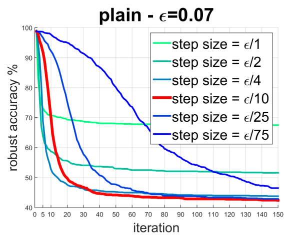
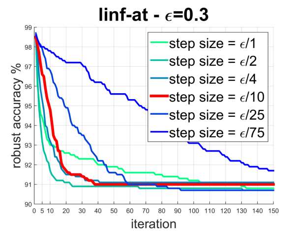
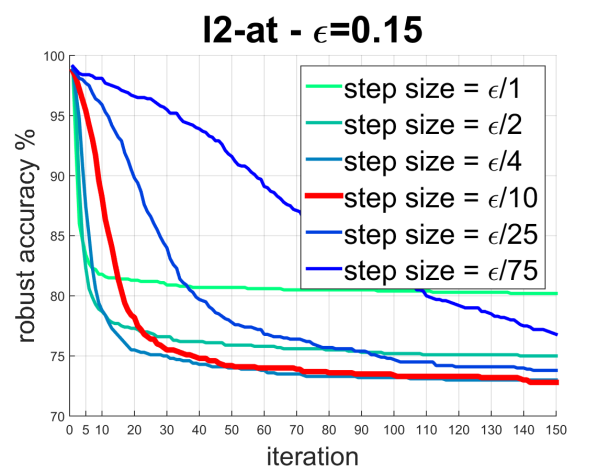
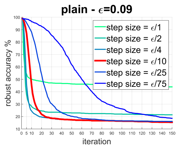
CIFAR-10 - $l_{\infty}$-attack

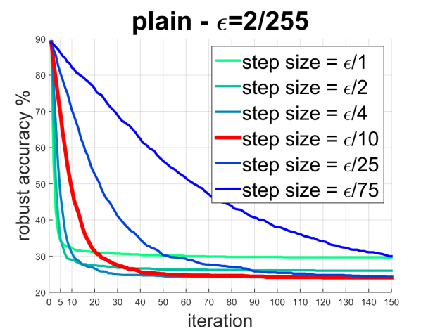
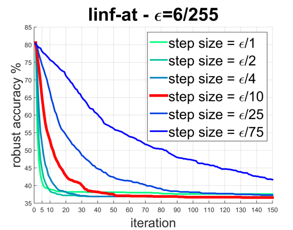
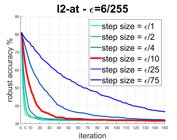
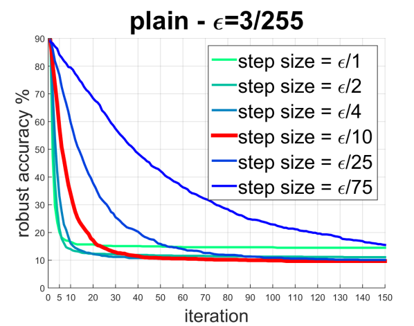
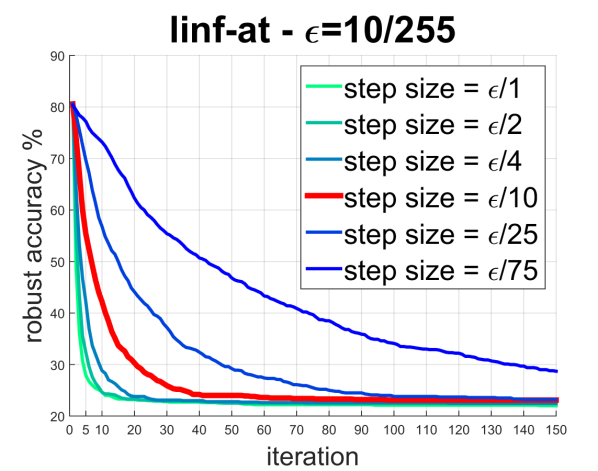
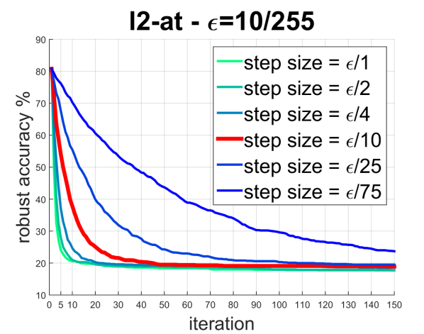
Figure 4: Evolution of robust accuracy as a function of the iterations for different step sizes for PGD wrt $l_{\infty}$. In red the step size we used in the experiments of Section 3. The models used are those trained on MNIST (top row) and CIFAR-10 (bottom row).

MNIST - $l_{2}$-attack

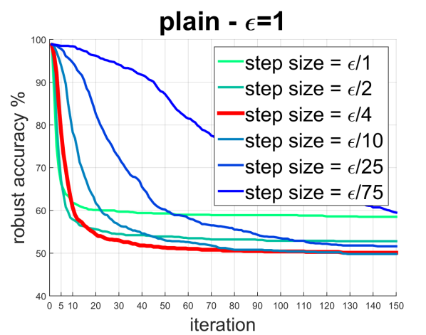
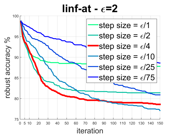
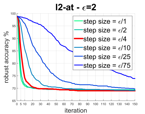
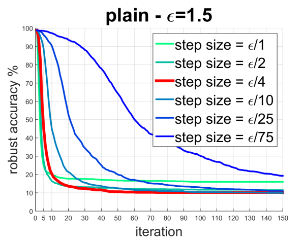
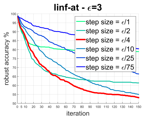
CIFAR-10 - $l_{2}$-attack

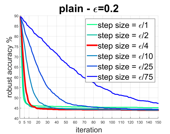
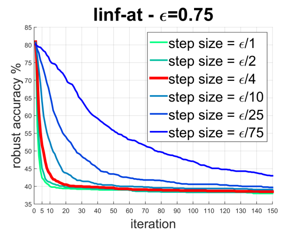
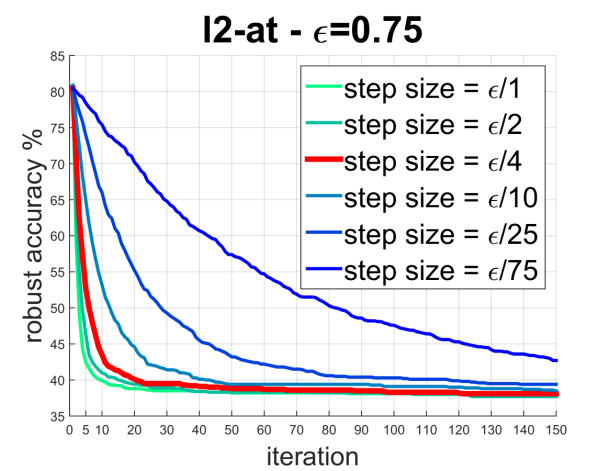
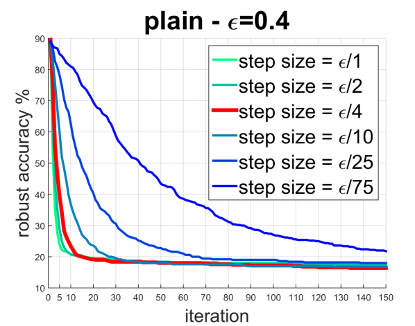
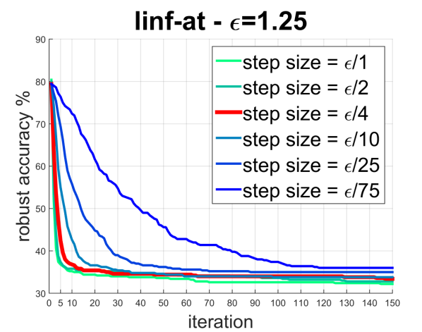
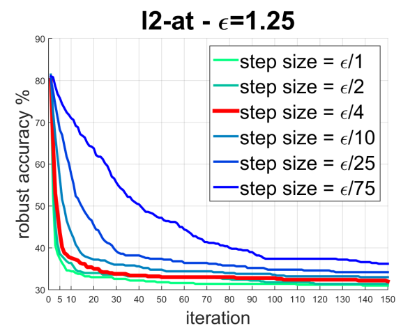
Figure 5: Evolution of robust accuracy as a function of the iterations for different step sizes for PGD wrt $l_{2}$. In red the step size we used in the experiments of Section 3. The models used are those trained on MNIST (top row) and CIFAR-10 (bottom row).

MNIST - $l_{1}$-attack

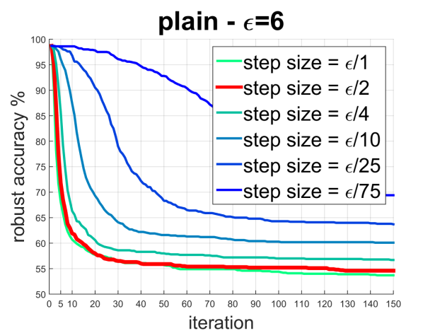
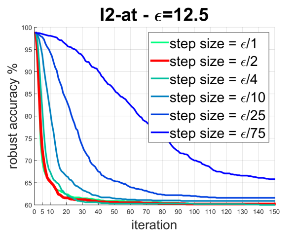
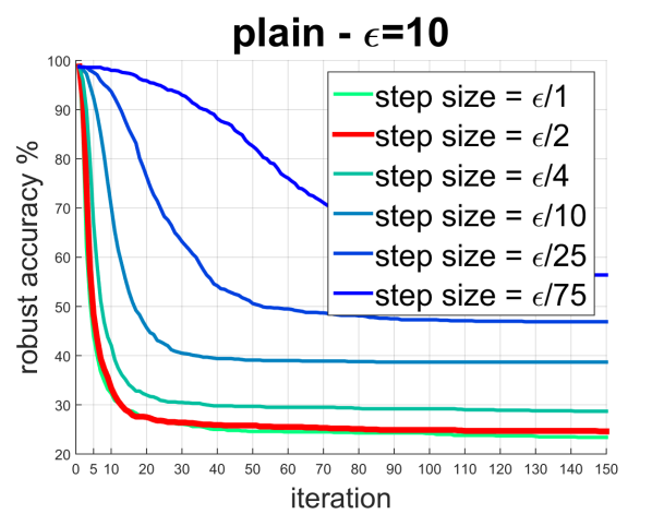
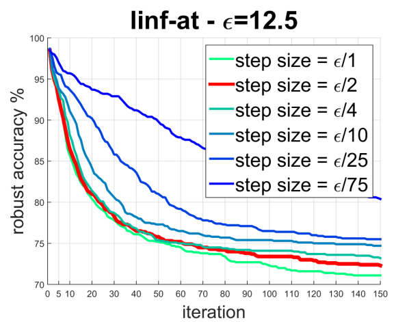
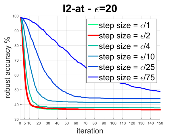
CIFAR-10 - $l_{1}$-attack

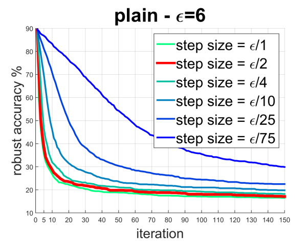
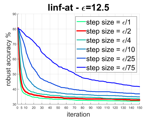
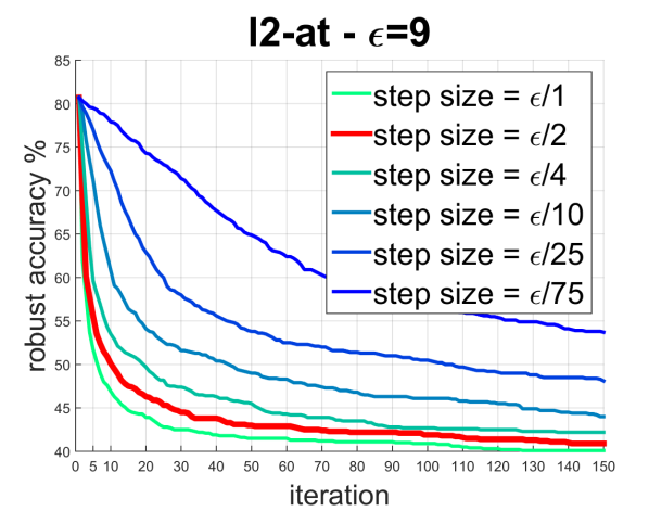
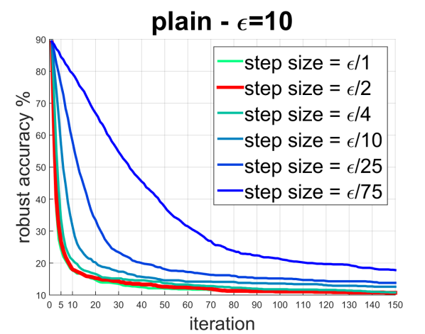
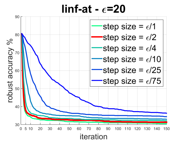
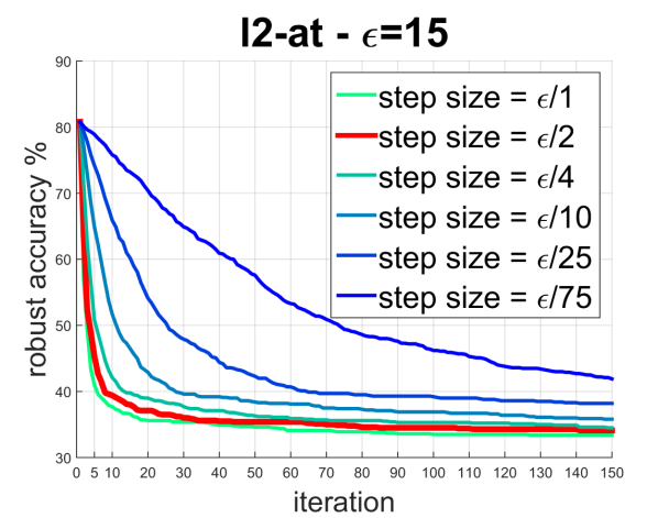
Figure 6: Evolution of robust accuracy as a function of the iterations for different step sizes for PGD wrt $l_{1}$. In red the step size we used in the experiments of Section 3. The models used are those trained on MNIST (top row) and CIFAR-10 (bottom row).

C.1 Choice of the step size of PGD

We here show the performance of PGD wrt $l_{1},l_{2},l_{\infty}$ on MNIST (top row of Figure 5) and CIFAR-10 (bottom row of Figure 5) for different choices of the step size. In particular we focus on large $\epsilon$. We report the robust accuracy as a function of iterations (in total 150 iterations). We test step sizes $\nicefrac{{\epsilon}}{{t}}$ for $t\in\{1,2,4,10,25,75\}$. For each step size we show the best run out of 10, with random initialization, which achieve the lowest robust accuracy after 150 iterations.

• $l_{2}$: In Figure 5 we show, for each dataset, the results for the three models used in Section 3, with decreasing step size corresponding to darker shades of blue, while our chosen step size for $l_{2}$, that is $\nicefrac{{\epsilon}}{{4}}$, is highlighted in red. We see that it achieves in all the models best or close to best robust accuracy.

• $l_{\infty}$: We show in Figure 4 the same plots as for $l_{2}$ but instead for $l_{\infty}$, the chosen stepsize $\nicefrac{{\epsilon}}{{10}}$ for $l_{\infty}$-attacks is highlighted in red. Again, we see that it is on average performing best.

• $l_{1}$: We show in Figure 6 the same plots as for $l_{2}$ but instead for $l_{1}$, the chosen stepsize $\nicefrac{{\epsilon}}{{2}}$ for $l_{1}$-attacks is highlighted in red. Again, we see that it is on average performing best.

MNIST, $l_{\infty}$

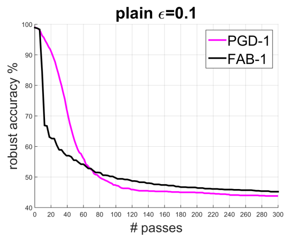
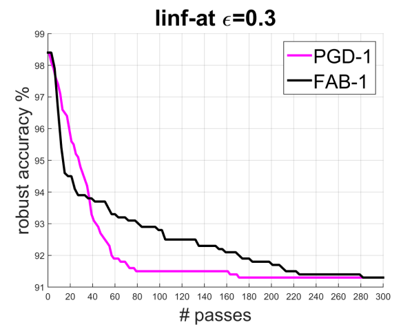
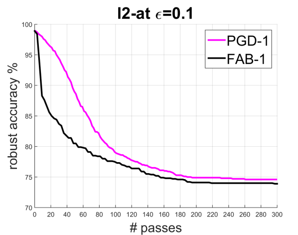
MNIST, $l_{2}$

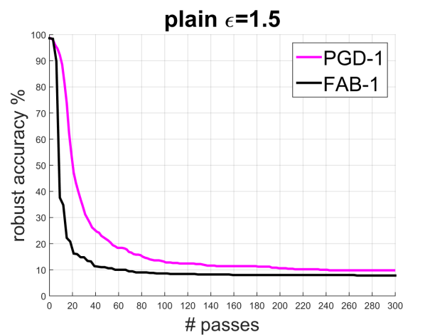
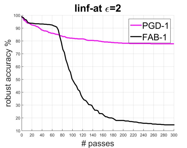
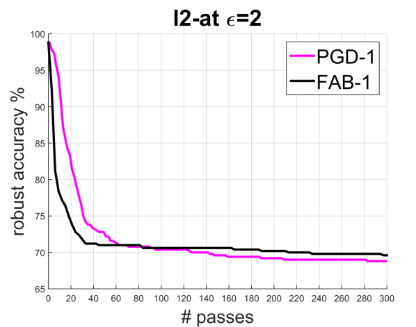
MNIST, $l_{1}$

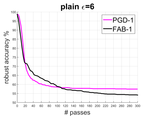
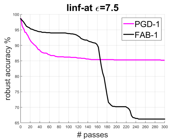
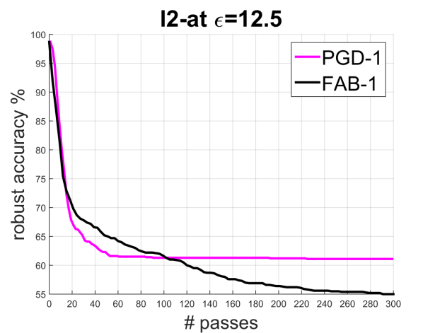
Figure 7: Evolution of robust accuracy as a function of the employed forward/backward passes on MNIST to ensure a fair comparison of PGD and FAB. We compare PGD-1 (magenta) and FAB-1 (black). Models: plain in the first column, $l_{\infty}$-at in the second and $l_{2}$-at in the third. Threat models: $l_{\infty}$ in the first row, $l_{2}$ in the second and $l_{1}$ in the third. The thresholds $\epsilon$ used can be read above the plots.

CIFAR-10, $l_{\infty}$

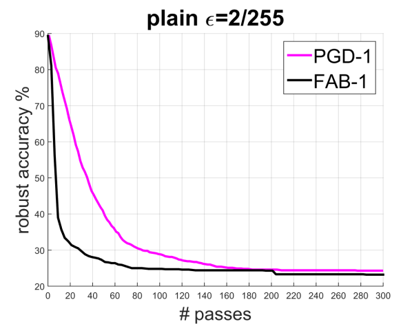
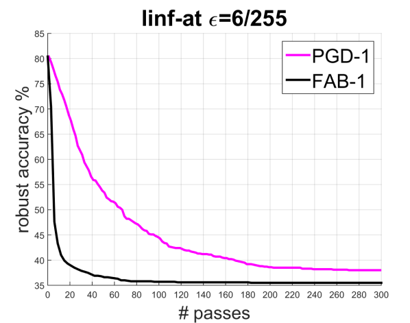
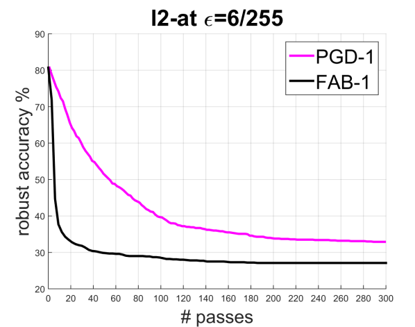
CIFAR-10, $l_{2}$

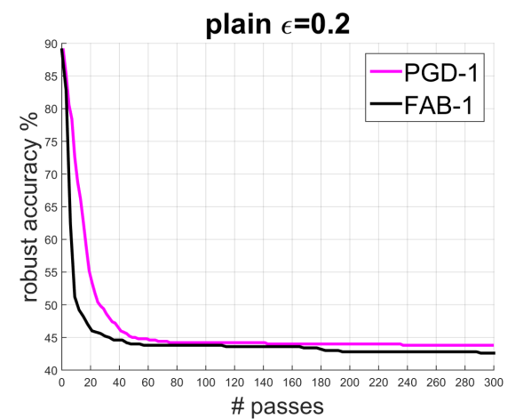
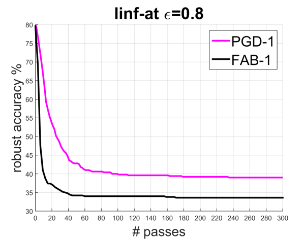
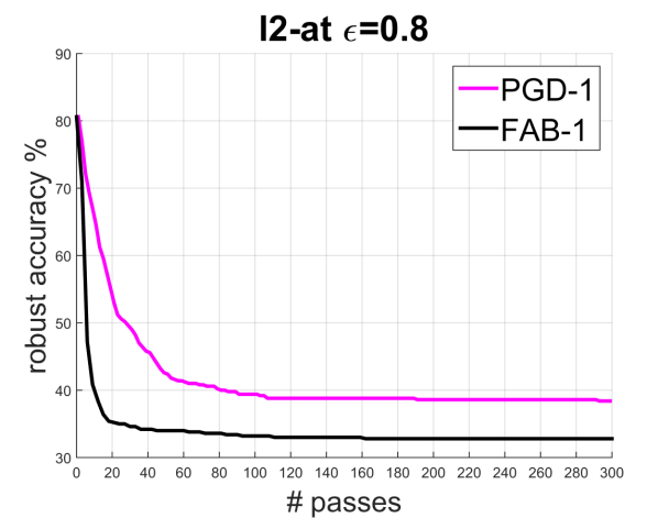
CIFAR-10, $l_{1}$

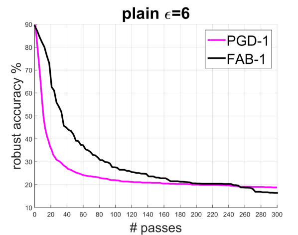
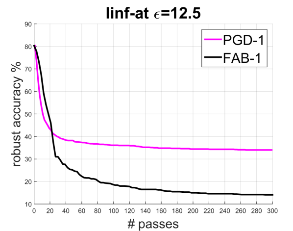
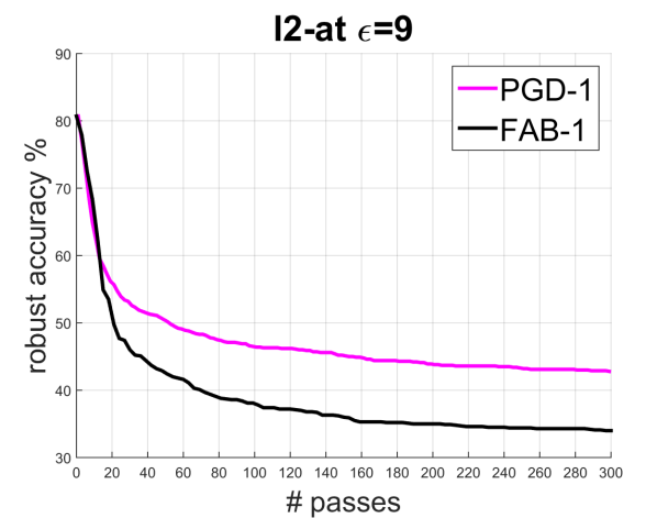
Figure 8: Evolution of robust accuracy as a function of the employed forward/backward passes on CIFAR-10 to ensure a fair comparison of PGD and FAB. We compare PGD-1 (magenta) and FAB-1 (black). Models: plain in the first column, $l_{\infty}$-at in the second and $l_{2}$-at in the third. Threat models: $l_{\infty}$ in the first row, $l_{2}$ in the second and $l_{1}$ in the third. The thresholds $\epsilon$ used can be read above the plots.

Restricted ImageNet, $l_{\infty}$

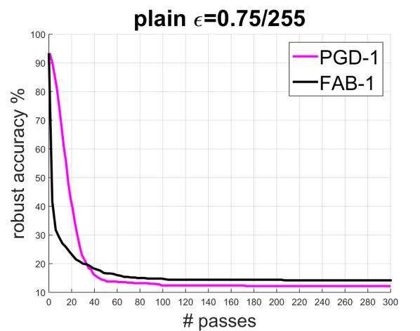
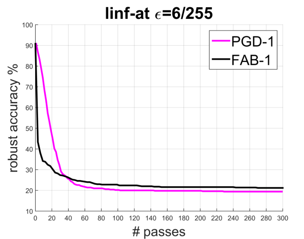
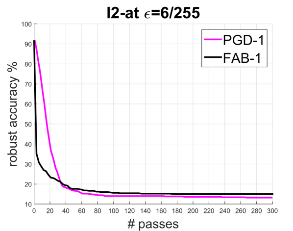
Restricted ImageNet, $l_{2}$

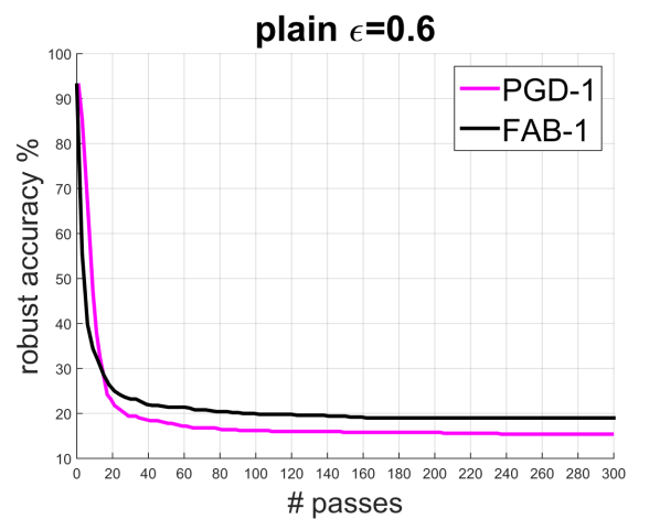
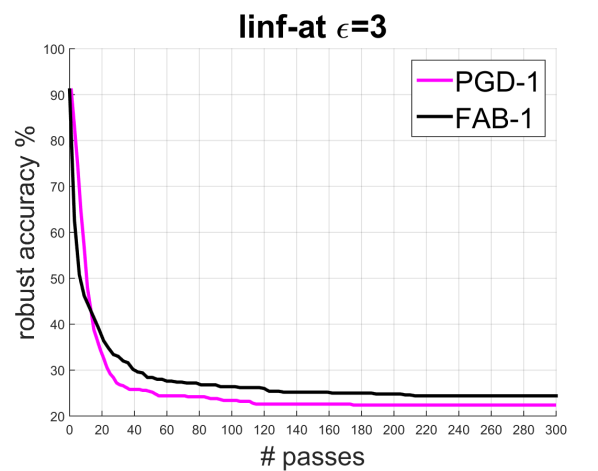
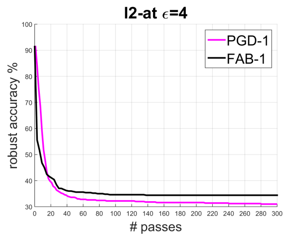
Restricted ImageNet, $l_{1}$

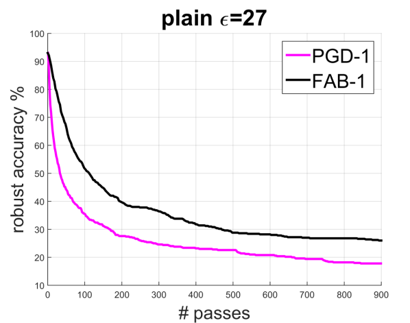
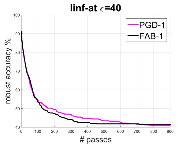
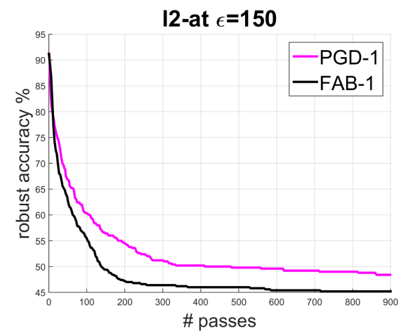
Figure 9: Evolution of robust accuracy as a function of the employed forward/backward passes on Restricted ImageNet to ensure a fair comparison of PGD and FAB. We compare PGD-1 (magenta) and FAB-1 (black). Models: plain in the first column, $l_{\infty}$-at in the second and $l_{2}$-at in the third. Threat models: $l_{\infty}$ in the first row, $l_{2}$ in the second and $l_{1}$ in the third. The thresholds $\epsilon$ used can be read above the plots.

C.2 Evolution across iteration

We compare the evolution of the robust accuracy across the iterations of PGD-1 (random starting point) and FAB-1 (starting at the target point $x_{\textrm{orig}}$). for the models and datasets from 7 to 15. Since PGD performs 1 forward and 1 backward pass for each iteration and FAB 2 forward passes and 1 backward pass, we rescale the robust accuracy so to compare the two methods when they have used exactly the same number of passes of the network. Then 300 passes correspond to 150 iterations of PGD and to 100 of FAB. In Figures 7, 8 and 9 we show the evolution of robust accuracy for the different datasets, models and threat models ($l_{\infty}$, $l_{2}$ and $l_{1}$), computed at two thresholds $\epsilon$ among the five used in Tables 7 to 15. One can see how FAB achieves in most of the cases good results within a few iterations, often faster than PGD.

References

- Athalye et al. (2018) Athalye, A., Carlini, N., and Wagner, D. A. Obfuscated gradients give a false sense of security: Circumventing defenses to adversarial examples. In ICML, 2018.
- Bastani et al. (2016) Bastani, O., Ioannou, Y., Lampropoulos, L., Vytiniotis, D., Nori, A., and Criminisi, A. Measuring neural net robustness with constraints. In NeurIPS, 2016.
- Brendel et al. (2018) Brendel, W., Rauber, J., and Bethge, M. Decision-based adversarial attacks: Reliable attacks against black-box machine learning models. In ICLR, 2018.
- Brown et al. (2017) Brown, T. B., Mané, D., Roy, A., Abadi, M., and Gilmer, J. Adversarial patch. In NeurIPS 2017 Workshop on Machine Learning and Computer Security, 2017.
- Carlini & Wagner (2017a) Carlini, N. and Wagner, D. Towards evaluating the robustness of neural networks. In IEEE Symposium on Security and Privacy, 2017a.
- Carlini & Wagner (2017b) Carlini, N. and Wagner, D. Adversarial examples are not easily detected: Bypassing ten detection methods. In ACM Workshop on Artificial Intelligence and Security, 2017b.
- Chen et al. (2018) Chen, P., Sharma, Y., Zhang, H., Yi, J., and Hsieh, C. Ead: Elastic-net attacks to deep neural networks via adversarial examples. In AAAI, 2018.
- Croce & Hein (2020) Croce, F. and Hein, M. Reliable evaluation of adversarial robustness with an ensemble of diverse parameter-free attacks. In ICML, 2020.
- Croce et al. (2019) Croce, F., Rauber, J., and Hein, M. Scaling up the randomized gradient-free adversarial attack reveals overestimation of robustness using established attacks. International J. of Computer Vision (IJCV), 2019.
- Engstrom et al. (2017) Engstrom, L., Tran, B., Tsipras, D., Schmidt, L., and Madry, A. A rotation and a translation suffice: Fooling CNNs with simple transformations. In NeurIPS 2017 Workshop on Machine Learning and Computer Security, 2017.
- Gu & Rigazio (2015) Gu, S. and Rigazio, L. Towards deep neural network architectures robust to adversarial examples. In ICLR Workshop, 2015.
- He et al. (2016) He, K., Zhang, X., Ren, S., and Sun, J. Deep residual learning for image recognition. In CVPR, pp. 770–778, 2016.
- Hein & Andriushchenko (2017) Hein, M. and Andriushchenko, M. Formal guarantees on the robustness of a classifier against adversarial manipulation. In NeurIPS, 2017.
- Huang et al. (2016) Huang, R., Xu, B., Schuurmans, D., and Szepesvari, C. Learning with a strong adversary. In ICLR, 2016.
- Katz et al. (2017) Katz, G., Barrett, C., Dill, D., Julian, K., and Kochenderfer, M. Reluplex: An efficient smt solver for verifying deep neural networks. In CAV, 2017.
- Krizhevsky et al. (2014) Krizhevsky, A., Nair, V., and Hinton, G. Cifar-10 (canadian institute for advanced research). 2014. URL http://www.cs.toronto.edu/~kriz/cifar.html.
- Kurakin et al. (2017) Kurakin, A., Goodfellow, I. J., and Bengio, S. Adversarial examples in the physical world. In ICLR Workshop, 2017.
- Madry et al. (2018) Madry, A., Makelov, A., Schmidt, L., Tsipras, D., and Valdu, A. Towards deep learning models resistant to adversarial attacks. In ICLR, 2018.
- Modas et al. (2019) Modas, A., Moosavi-Dezfooli, S., and Frossard, P. Sparsefool: a few pixels make a big difference. In CVPR, 2019.
- Moosavi-Dezfooli et al. (2016) Moosavi-Dezfooli, S.-M., Fawzi, A., and Frossard, P. Deepfool: a simple and accurate method to fool deep neural networks. In CVPR, pp. 2574–2582, 2016.
- Mosbach et al. (2018) Mosbach, M., Andriushchenko, M., Trost, T., Hein, M., and Klakow, D. Logit pairing methods can fool gradient-based attacks. In NeurIPS 2018 Workshop on Security in Machine Learning, 2018.
- Narodytska & Kasiviswanathan (2016) Narodytska, N. and Kasiviswanathan, S. P. Simple black-box adversarial perturbations for deep networks. In CVPR 2017 Workshops, 2016.
- Pang et al. (2020) Pang, T., Xu, K., Dong, Y., Du, C., Chen, N., and Zhu, J. Rethinking softmax cross-entropy loss for adversarial robustness. In ICLR, 2020.
- Papernot et al. (2016) Papernot, N., McDonald, P., Wu, X., Jha, S., and Swami, A. Distillation as a defense to adversarial perturbations against deep networks. In IEEE Symposium on Security & Privacy, 2016.
- Papernot et al. (2017) Papernot, N., Carlini, N., Goodfellow, I., Feinman, R., Faghri, F., Matyasko, A., Hambardzumyan, K., Juang, Y.-L., Kurakin, A., Sheatsley, R., Garg, A., and Lin, Y.-C. cleverhans v2.0.0: an adversarial machine learning library. preprint, arXiv:1610.00768, 2017.
- Rauber et al. (2017) Rauber, J., Brendel, W., and Bethge, M. Foolbox: A python toolbox to benchmark the robustness of machine learning models. In ICML Reliable Machine Learning in the Wild Workshop, 2017.
- Su et al. (2019) Su, J., Vargas, D. V., and Kouichi, S. One pixel attack for fooling deep neural networks. IEEE Transactions on Evolutionary Computation, 23:828–841, 2019.
- Tjeng et al. (2019) Tjeng, V., Xiao, K., and Tedrake, R. Evaluating robustness of neural networks with mixed integer programming. In ICLR, 2019.
- Tramèr & Boneh (2019) Tramèr, F. and Boneh, D. Adversarial training and robustness for multiple perturbations. In NeurIPS, 2019.
- Tsipras et al. (2019) Tsipras, D., Santurkar, S., Engstrom, L., Turner, A., and Madry, A. Robustness may be at odds with accuracy. In ICLR, 2019.
- Wong et al. (2019) Wong, E., Schmidt, F. R., and Kolter, J. Z. Wasserstein adversarial examples via projected sinkhorn iterations. In ICML, 2019.
- Zheng et al. (2016) Zheng, S., Song, Y., Leung, T., and Goodfellow, I. J. Improving the robustness of deep neural networks via stability training. In CVPR, 2016.
- Zheng et al. (2019) Zheng, T., Chen, C., and Ren, K. Distributionally adversarial attack. In AAAI, 2019.