Enhancing Sensitivity to Non-Standard Neutrino Interactions at INO combining muon and hadron information
Abstract
The neutral current non-standard interactions (NSI’s) of neutrino with matter fermions while propagating through long distances inside the Earth matter can give rise to the extra matter potentials apart from the standard MSW potential due to the -mediated interactions in matter. In this paper, we explore the impact of flavor violating neutral current NSI parameter in the oscillation of atmospheric neutrino and antineutrino using the 50 kt magnetized ICAL detector at INO. We find that due to non-zero , and transition probabilities get modified substantially at higher energies and longer baselines, where vacuum oscillation dominates. We estimate the sensitivity of the ICAL detector for various choices of binning schemes and observables. The most optimistic bound on that we obtain is at 90 C.L. using 500 ktyr exposure and considering as observables in their ranges [1, 21] GeV, [-1, 1], and [0, 25] GeV respectively. For the first time we show that the charge identification capability of the ICAL detector is crucial to set stringent constraints on . We also show that when we marginalize over in fit in its range of -0.1 to 0.1, the mass hierarchy sensitivity deteriorates by 10 to 20 depending on the analysis mode, and the precision measurements of atmospheric parameters remain quite robust at the ICAL detector.
Keywords:
Non-Standard Interactions, Atmospheric Neutrinos, Precision Measurement, Mass Hierarchy, ICAL, INO, Muon1 Introduction
The observation of neutrino oscillation proves that the neutrinos are massive and mix with each other, which is the first direct evidence for physics beyond the Standard Model Olive:2016xmw . Currently, the three-flavor lepton mixing is confirmed and neutrino oscillation has entered the era of precision Capozzi:2017ipn ; Esteban:2018azc ; deSalas:2017kay . To explain the tiny masses of neutrino and large leptonic mixing angles, the extensions of the Standard Model allow some interactions which are not possible in the Standard Model. These interactions are termed as non-standard interactions (NSI’s). The presence of NSI’s in nature can have subdominant effect on the oscillation of neutrino and antineutrino. Therefore, the phenomenological consequences of NSI’s in three-flavor mixing using neutrino oscillation experiments are interesting and widely studied by many authors in Refs. GonzalezGarcia:1998hj ; Bergmann:1998rg ; Bergmann:1999rz ; Lipari:1999vh ; Guzzo:2000kx ; GonzalezGarcia:2001mp ; Gago:2001xg ; Berezhiani:2001rs ; Huber:2001zw ; Fornengo:2001pm ; Huber:2002bi ; Gago:2001si ; Berezhiani:2001rt ; Ota:2001pw ; Davidson:2003ha ; Friedland:2004ah ; GonzalezGarcia:2004wg ; Guzzo:2004ue ; Friedland:2005vy ; Kitazawa:2006iq ; Mangano:2006ar ; Blennow:2005qj ; EstebanPretel:2007yu ; Barranco:2007tz ; Ribeiro:2007ud ; Kopp:2007mi ; Blennow:2008ym ; EstebanPretel:2008qi ; Barranco:2007ej ; Kopp:2007ne ; Blennow:2007pu ; Ohlsson:2008gx ; Gavela:2008ra ; Bolanos:2008km ; Antusch:2008tz ; Biggio:2009nt ; Escrihuela:2009up ; Gago:2009ij ; Biggio:2009kv ; Oki:2010uc ; Kopp:2010qt ; Forero:2011zz ; Escrihuela:2011cf ; GonzalezGarcia:2011my ; Coloma:2011rq ; Adhikari:2012vc ; Agarwalla:2012wf ; Gonzalez-Garcia:2013usa ; Ohlsson:2013epa ; Ohlsson:2012kf ; Choubey:2015xha ; Farzan:2017xzy .
In this paper, we study the impact of neutral current (NC) non-standard interactions of neutrino which may arise when atmospheric neutrinos travel long distances inside the Earth. While NC NSI’s affect neutrinos during their propagation, there are charged-current NSI’s which may modify the neutrino fluxes at the production stage and interaction cross-section at the detection level. In this work, we only focus on the NC NSI’s, and do not consider NSI’s at production and detection level. In most of the cases, NSI’s come into the picture as a low-energy manifestation of high-energy theory involving new heavy states. For a detailed discussion on this topic, see the reviews Biggio:2009nt ; Ohlsson:2012kf ; Miranda:2015dra ; Farzan:2017xzy . Therefore, at low energies, a neutral current NSI can be described by a four-fermion dimension-six operator Wolfenstein:1977ue ,
| (1) |
where is the Fermi coupling constant, is the dimensionless parameter which represents the strength of NSI relative to , and and are the neutrino fields of flavor and respectively. Here, denotes the matter fermions, electron (), up-quark (), and down-quark (). Here, , , and the subscript expresses the chirality of the current. Due to the hermiticity of the interaction, we have .
The NSI’s of neutrino with matter fermions can give rise to the additional matter induced potentials apart from the standard MSW potential due to the -mediated interactions in matter as denoted by . The total relative strength of the matter induced potential generated by the NC NSI’s of neutrinos with all the matter fermions () can be written in the following fashion,
| (2) |
where = , . The quantity denotes the number density of matter fermion in the medium. For antineutrino, and . In general, the total matter induced potential in presence of all the possible NC non-standard interactions of neutrino with matter fermions can be written as
| (3) |
In the present study, we focus our investigation to flavor violating NSI parameter , that is, we only allow to be non-zero in our analysis, and assume all other NSI parameters to be zero. We also consider to be real entertaining both of its negative and positive values. Since the atmospheric neutrino oscillation is mainly governed by transition, it is expected that NSI parameter would have significant impact on this oscillation channel, which in turn can modify survival probability by a considerable amount. We can study this effect by observing the atmospheric neutrinos at the proposed 50 kt magnetized ICAL detector. If we will not see any significant deviation from the standard and event spectra at ICAL, we can use this fact to place tight constraints on NSI parameter . This is the main theme of our present study.
This article is organized in the following fashion. In Sec. 2, we briefly review the existing bounds on NSI parameter from various neutrino oscillation experiments. We discuss the possible modification in oscillation probabilities of neutrino and antineutrino due to non-zero in Sec. 3. In Sec. 4, we present the expected total and events and their distributions as a function of reconstructed and for the following three cases: (i) (SM), (ii) , and (iii) using 500 ktyr exposure of the ICAL detector. In Sec. 5, we discuss the numerical procedure and various binning schemes that we use in our analysis. We present all the results of our study in Sec. 6 where we show the following: (a) The possible improvement in the sensitivity of the ICAL detector in constraining due to the inclusion of events with in range of 11 to 21 GeV in addition to the events that belong to the in range of 1 to 11 GeV. (b) How much the limit on can be improved by considering the information on reconstructed hadron energy () as an additional observable along with reconstructed variables and on an event-by-event basis. (c) We show the advantage of having charge identification (CID) capability in the ICAL detector in placing competitive constraint on . (d) We present the expected limits on considering different exposures of the 50 kt ICAL detector. (e) We also explore the possible impact of non-zero in determining the mass hierarchy and in the precision measurement of atmospheric oscillation parameters. We provide a summary of this study in Sec. 7.
2 Existing Limits on NSI Parameter
There are existing constraints on the NSI parameter from various neutrino oscillation experiments. The Super-Kamiokande collaboration performed an analysis of the atmospheric neutrino data collected during its phase-I and -II run assuming only NSI’s with -quarks Mitsuka:2011ty . The following bounds at C.L. are obtained:
| (4) |
Since for an electrically neutral and isoscalar Earth matter, the above constraints as obtained in Ref. Mitsuka:2011ty are actually on the NSI parameters . Therefore, the above constraints at C.L. can be interpreted as
| (5) |
Recently, the authors in Ref. Salvado:2016uqu considered the possibility of NSI’s in - sector in the one-year high-energy through-going muon data of IceCube. In their analysis, they included various systematic uncertainties on both the atmospheric neutrino flux and detector properties, which they incorporated via several nuisance parameters. They obtained the following limits
| (6) |
The IceCube-DeepCore collaboration also searched for NSI’s involving Aartsen:2017xtt . Using their three years of atmospheric muon neutrino disappearance data, they placed the following constraint at confidence level
| (7) |
A preliminary analysis to constrain the NSI parameters in context of the ICAL detector was performed in Ref. Choubey:2015xha . Using an exposure of 500 ktyr and considering only muon momentum () as observable, the authors in Ref. Choubey:2015xha obtained the following bound
| (8) |
In the present study, we estimate new constraints on considering the reconstructed hadron energy () as an additional observable along with the reconstructed and on an event-by-event basis at the ICAL detector.
3 transition with non-zero
This section is devoted to explore the effect of non-zero in the oscillation of atmospheric neutrino and antineutrino propagating long distances through the Earth matter. For this, we numerically estimate the three-flavor oscillation probabilities including NSI parameter and using the PREM profile Dziewonski:1981xy for the Earth matter density. The NSI parameter modifies the evolution of neutrino in matter, which in the flavor basis takes the following form,
| (9) |
where is real in our analysis.
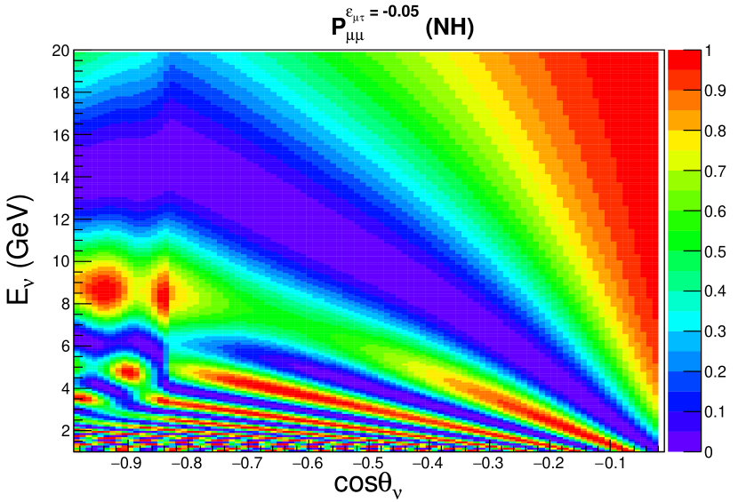
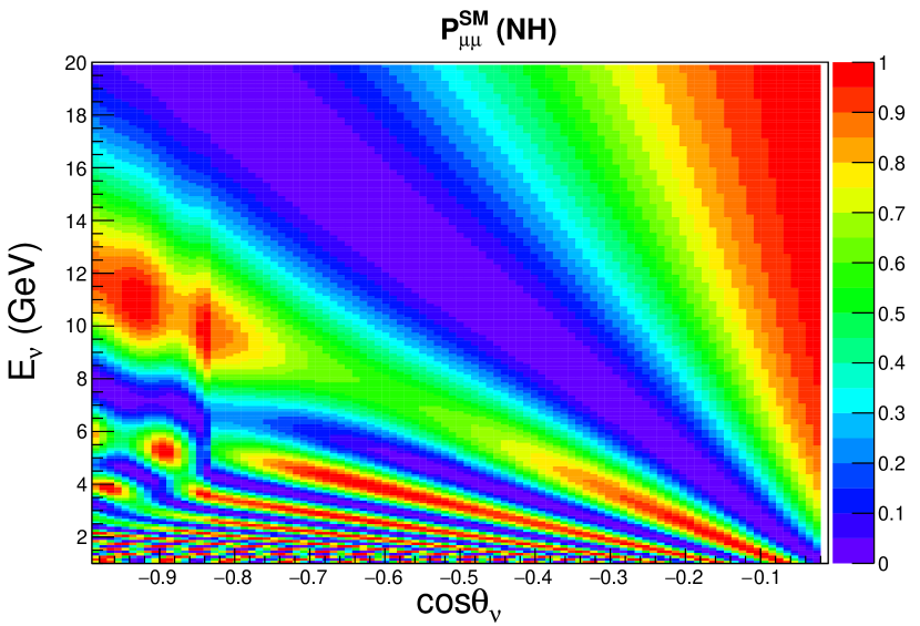
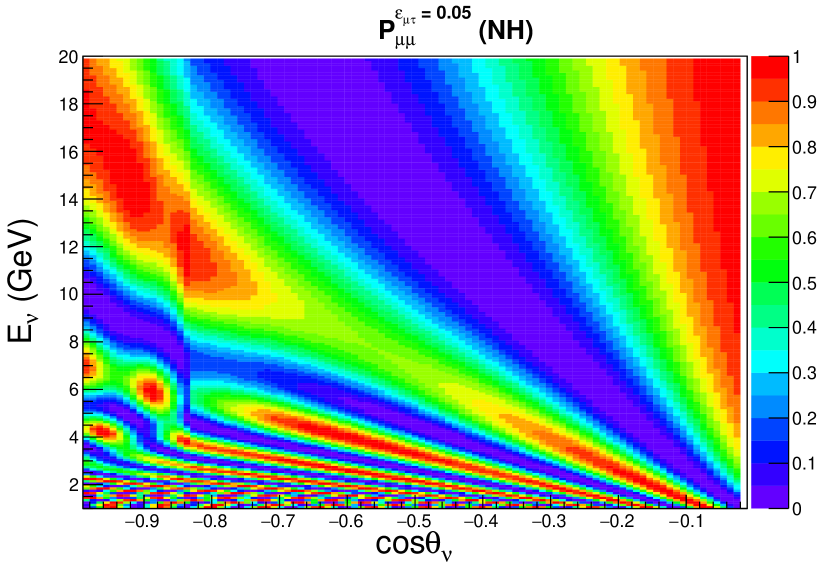
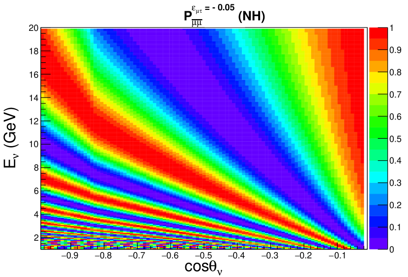
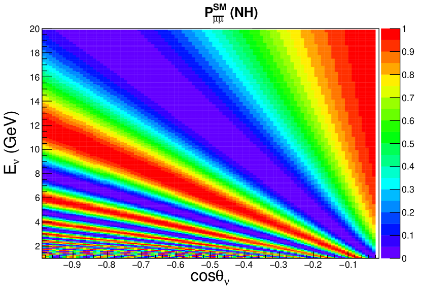
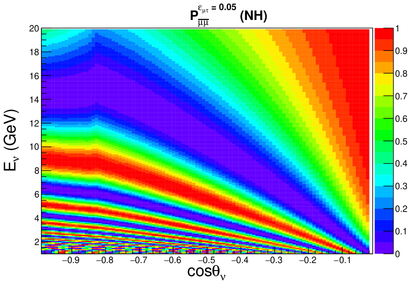
In upper panels of Fig. 1, we present the oscillograms for survival channel in the plane of vs. considering NH. Here, we draw the oscillograms for three different cases: i) (left panel), ii) (the SM case, middle panel), and iii) (right panel). The lower panel depicts the same but for oscillation channel. To prepare Fig. 1, we take the following benchmark values of vacuum oscillation parameters in three-flavor framework: , , , eV2, eV2, and . We estimate the value of from 111The effective mass splitting is related to as follows Nunokawa:2005nx ; deGouvea:2005hk (10) , where has the same magnitude for NH and IH with positive and negative signs respectively. It is evident from the upper panels of Fig. 1 that in the presence of negative (see left panel) and positive (see right panel) non-zero values of , survival probabilities get modified substantially at higher energies and longer baselines, where vacuum oscillation dominates. We observe the similar changes in case of oscillation probabilities as well (see lower panels).
Another broad feature which has been emerging from Fig. 1 is that the oscillation probabilities with positive (negative) as shown in upper right (left) panel are similar to that of transition probabilities with negative (positive) as can be seen from lower left (right) panel. We can understand this behaviour with the help of following approximate analytical expression of transition probability. Assuming and , oscillation channel in the presence of non-zero and under the constant matter density approximation takes the form Gago:2001xg ; GonzalezGarcia:2004wg
| (11) |
where
| (12) |
| (13) |
and
| (14) |
In Eqs. 12 and 13, positive and negative signs in front of are associated with the normal and inverted hierarchy respectively. In case of maximal mixing (), Eq. 11 boils down to the following simple expression Hollander:2014iha
| (15) |
Since for antineutrino, , following Eq. 15, we can write
| (16) |
and
| (17) |
Eq. 16 and Eq. 17 explain the broad features in Fig. 1 that we mention above.
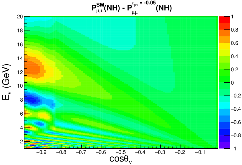
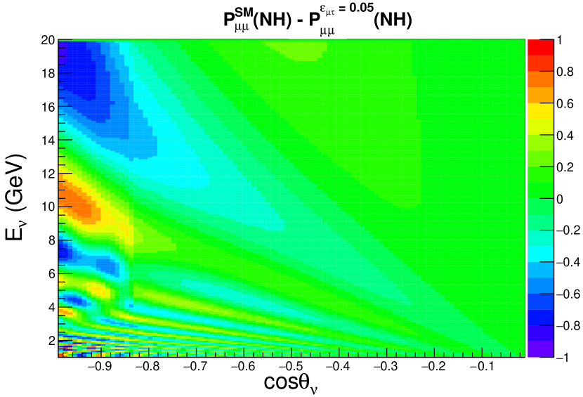

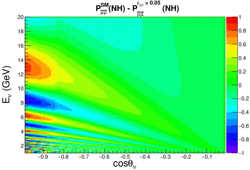
To have a better look at the changes induced by non-zero as compared to the SM case, we give Fig. 2 where we plot the difference in survival channel considering the cases (the SM case) and (see top left panel). In top right panel, we present the same for the cases of (the SM case) and . The lower panels are for antineutrinos. In all the panels, we see a visible difference in survival channel due to the presence of non-zero as compared to the SM case () at higher baselines with in the range to . This range of corresponds to the baseline in the range 12700 km to 10000 km where neutrino and antineutrino mostly travel through inner and outer part of the Earth’s core222According to a simplified version of the PREM profile Dziewonski:1981xy , the inner core has a radius of 1220 km with an average density of 13 g/cm3. For outer core, km and 3480 km with an average density of 11.3 g/cm3. Note that in our analysis, we consider the detailed version of the PREM. and have access to large Earth matter effect. Also, we see a trend that the impact of NSI’s is large at higher energies where the three-flavor oscillations are suppressed because the oscillation lengths () are large at higher energies.
To have a quantitative estimate of the difference in oscillation channel due to non-zero as compared to case, we use Eq. 15 and obtain the following expression
| (18) |
Eq. 18 clearly suggests that the impact of NSI is proportional to both NSI induced matter potential () and baseline (). We see in upper left and lower right panels of Fig. 2 that around GeV and , approaches to zero suggesting that the impact of NSI is negligible. We observe the opposite behaviour in upper right and lower left panels, where around GeV and , attains a quite large value of suggesting that the influence of NSI is significant there. Here, corresponds to km for which the line-averaged constant Earth matter density according to the PREM Dziewonski:1981xy profile is 6.8 g/cm3. Therefore, the standard line-averaged Earth matter potential333The standard neutrino matter potential due to the -mediated interactions with the ambient electrons can be written as a function of matter density as follows: (19) where () is the relative number density. For electrically, neutral and isoscalar medium, , and therefore, . for 11500 km baseline is eV. Considering , we get
| (20) |
For GeV, km, and eV2 (this mass-squared difference is obtained from Eq. 10 using benchmark values of oscillation parameters),
| (21) |
Thus, for GeV and km, from Eq. 18, we obtain
| (22) |
and
| (23) |
Eq. 22 and Eq. 23 confirm the observations regarding and in Fig. 2 that we mention above. We know that due to its CID capability, ICAL has an edge to resolve the issue of neutrino mass hierarchy (sign of ) by observing the Earth matter effect in and events separately Kumar:2017sdq . Similarly, the four panels in Fig. 2 suggest that the CID capability of ICAL can provide useful information to determine the sign of NSI parameter for a particular choice of mass hierarchy.
4 Expected Events at ICAL with non-zero
The Monte Carlo based neutrino event generator NUANCE Casper:2002sd is used to simulate the CC interactions of and in the ICAL detector. To generate events in NUANCE, we give a simple geometry of the ICAL detector with 150 alternate layers of iron and glass plates in each module. We have three such modules to account for the 50 kt ICAL detector. As far as the neutrino flux is concerned in generating the neutrino events in the present study, we use the flux as predicted at Kamioka444Preliminary calculation of the expected fluxes at the INO site has been performed in Ref. Athar:2012it ; Honda:2015fha . The visible differences between the neutrino fluxes at the Kamioka and INO sites appear at lower energies. The main reason behind this is that the horizontal components of the geo-magnetic field are different at the Kamioka (30T) and INO (40 T) locations. We plan to use these new fluxes estimated for the INO site (see Ref. Honda:2015fha ) in future studies. Honda:2011nf . To reduce the statistical fluctuation, we generate the unoscillated CC neutrino and antineutrino events considering a very high exposure of 1000 years and 50 kt ICAL. Then, we implement various oscillation probabilities using the reweighting algorithm. Next, we fold the oscillated events with detector response for muon and hadron as described in Ref. Chatterjee:2014vta ; Devi:2013wxa . In the present study, we assume that the ICAL particle reconstruction algorithms can separate the hits due to the hadron shower from the hits originating from a muon track with 100 efficiency. It means that whenever a muon is reconstructed, we consider all the other hits to be part of the hadronic shower in order to calibrate the hadron energy. It also implies that the neutrino event reconstruction efficiency is same as the muon reconstruction efficiency. Finally, the reconstructed and events are scaled down to the exposure of 10 years for 50 kt ICAL. Now, we present the expected and events for 500 ktyr exposure of the ICAL detector assuming the SM case () and . To estimate these event rates, we use the values of oscillation parameters as considered in Sec. 3 to draw the oscillograms.
4.1 Total Event Rates
First, we address the following question: can we see the signature of non-zero in the total number of and events which will be collected at the ICAL detector over 10 years of running? To have an answer of this question, we estimate the total number of events for the following three cases: i) , ii) (the SM case), and iii) . We present these numbers in Table 1 with NH and using 500 ktyr exposure of the ICAL detector integrating over entire ranges of , , and that we consider in our analysis.
| low-energy (LE) | high-energy (HE) | |||
| 0.05 | 4574 (total) 4474 () 100 () | 2029 (total) 2016 () 13 () | 4879 (total) 4778 () 101 () | 2192 (total) 2179 () 13 () |
| SM | 4562 (total) 4458 () 104 () | 2035 (total) 2022 () 13 () | 4870 (total) 4765 () 105 () | 2188 (total) 2175 () 13 () |
| -0.05 | 4553 (total) 4444 () 109 () | 2037 (total) 2024 () 13 () | 4890 (total) 4780 () 110 () | 2191 (total) 2178 () 13 () |
As far as the binning schemes are concerned, we use the low-energy (LE) and high-energy (HE) binning schemes555For a detailed description of the two binning schemes that we consider in our analysis, see Sec. 5.1., and for both these binning schemes, we take the entire range of spanning over -1 to 1. The energy ranges for reconstructed and are different in LE and HE binning schemes. For LE binning scheme, [1, 11] GeV and [0, 15] GeV. In case of HE binning scheme, [1, 21] GeV, and [0, 25] GeV. When we increase the reconstructed muon energy from 11 GeV to 21 GeV and reconstructed hadron energy from 15 GeV to 25 GeV, the number of and events get increased by 300 and 150 respectively for 500 ktyr exposure of the ICAL detector. Apart from showing the total event rates in Table 1, we also present the estimates of individual events coming from () disappearance channel and () appearance channel. Also, for events, we separately show the contributions originating from () disappearance and () appearance channels. Here, we see that only of the total events at the ICAL detector come via the appearance channel. Note that the differences in the total number of and events between the SM case () and non-zero of are not significant. But, later while presenting our final results, we see that the ICAL detector can place competitive constraints on by exploiting the useful information contained in the spectral distributions of and events as a function of reconstructed observables , , and . To establish this claim, now, we show how the expected and event spectra get modified in the presence of non-zero in terms of reconstructed and while integrating over entire range of .
4.2 Event Spectra
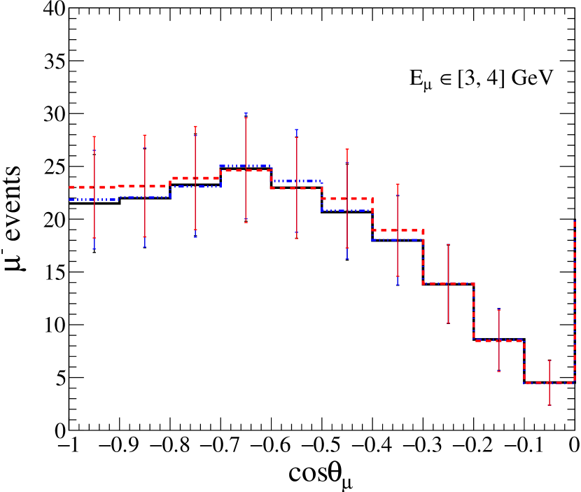
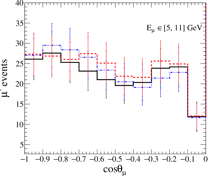
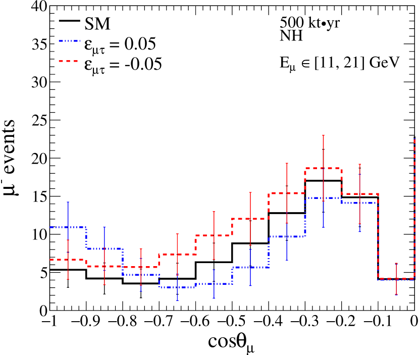
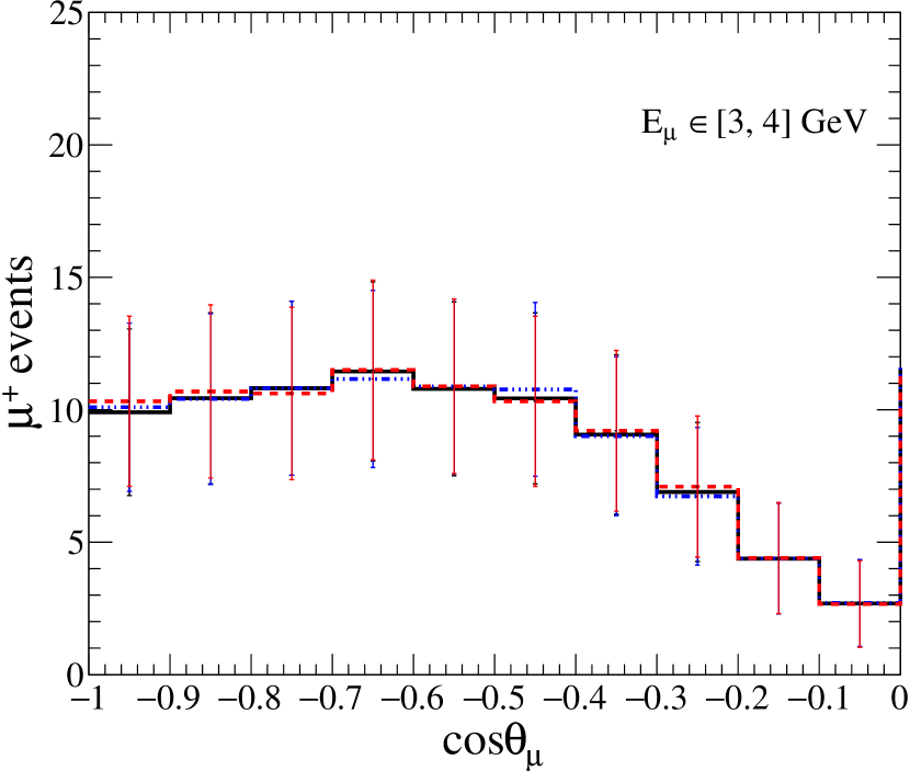
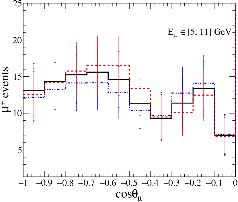
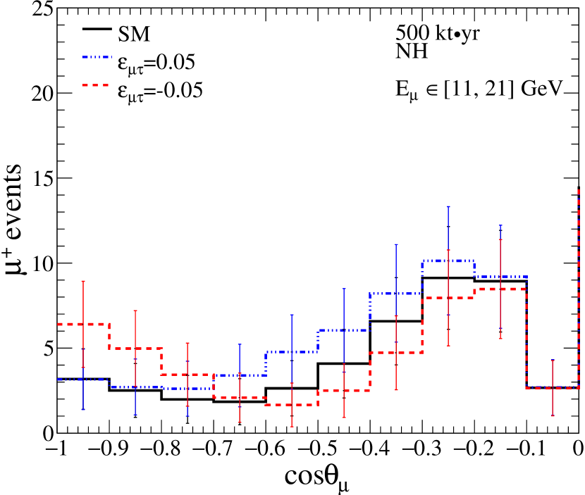
In Fig. 3, we show the distributions of (upper panels) and (lower panels) events as a function of reconstructed for three different ranges of . The ranges of that we consider in left, middle, and right panels are [3, 4] GeV, [5, 11] GeV, and [11, 21] GeV respectively. Here, we integrate over in its entire range of 0 to 25 GeV. In each panel, we compare the event spectra for three different cases: i) (blue line), ii) (the SM case, black line), and iii) (red line). Before we discuss the impact of non-zero , we would like to mention few general features that are emerging from various panels in Fig. 3. For both (upper panels) and (lower panels), the number of events get reduced as we go to higher energies. It happens because of dependence of the atmospheric neutrino flux. Though the neutrino fluxes are higher along the horizontal direction ( around ) as compared to the other directions (for detailed discussion, see Ref. Honda:2015fha ), but, due to the poor reconstruction efficiency of the ICAL detector along the horizontal direction Chatterjee:2014vta , we see a suppression in and event rates around irrespective of the choices of ranges. Important to note that as we proceed towards higher , the relative differences in and event rates between the SM case () and non-zero () get increased for a wide range of . We see similar features in Fig. 2 in Sec. 3, where we show the differences in oscillograms due to the SM case () and non-zero (). We show the improvement in the sensitivity to constrain due to high energy events in Sec. 6.1. Next, we discuss the numerical technique and analysis procedure which we adopt to obtain the final results.
5 Simulation Method
5.1 Binning Scheme in (, , ) Plane
In the present study, we produce all the results with low-energy (LE) and high-energy (HE) binning schemes. Table 2 shows the detailed information about the LE binning scheme for the three reconstructed observables , , and . Table 3 portrays the same for the HE binning scheme. In case of LE binning scheme, the range of is [1, 11] GeV with total 10 bins each having a width of 1 GeV. In case of HE binning scheme, we extend the range of up to 21 GeV by adding two additional bins in the range of 11 to 21 GeV, where each bin has a width of 5 GeV. As far as reconstructed is concerned, in case of LE (HE) binning scheme, the considered range is 0 to 15 GeV (0 to 25 GeV). We can see from Table 2 and Table 3 that the first three bins for are same for both the binning schemes, whereas the last bin extend from 4 to 15 GeV (4 to 25 GeV) for LE (HE) binning scheme. For both these binning schemes, we consider the entire range of from -1 to 1. For upward going events, that is [-1, 0], we consider 10 uniform bins each having width of 0.1. For downward going events, that is [0, 1], we consider 5 uniform bins each having width of 0.2. Important to note that the downward going events do not have enough path length to oscillate, but, these events play an important role to increase the overall statistics and to minimize the effect of normalization uncertainties in atmospheric neutrino fluxes. Here, we would like to mention that we have not optimized these binning schemes to obtain the best sensitivities, but we ensure that there are sufficient statistics in most of the bins.
| Observable | Range | Bin width | No. of bins | Total bins |
| (GeV) | 1 | 10 | 10 | |
| 0.1 0.2 | 10 5 | 15 | ||
| (GeV) | 1 2 11 | 2 1 1 | 4 |
| Observable | Range | Bin width | No. of bins | Total bins |
| (GeV) | 1 5 | 10 2 | 12 | |
| 0.1 0.2 | 10 5 | 15 | ||
| (GeV) | 1 2 21 | 2 1 1 | 4 |
5.2 Numerical Analysis
In our analysis, the function gives us the median sensitivity of the experiment in the frequentist approach Blennow:2013oma . We use the following Poissonian for events in our statistical analysis considering , , and as observables (the so-called “3D” analysis as considered in Devi:2014yaa ):
| (24) |
with
| (25) |
In the above equations, and denote the observed and expected number of events in a given [, , ] bin. In case of LE (HE) binning scheme, = 10 (12), , and . In Eq. 25, represents the number of expected events without systematic uncertainties. Following Ref. Ghosh:2012px , we consider five systematic errors in our analysis: 20 flux normalization error, 10 error in cross-section, 5 tilt error, 5 zenith angle error, and 5 overall systematics. We incorporate these systematic uncertainties in our simulation using the well known “pull” method Huber:2002mx ; Fogli:2002pt ; GonzalezGarcia:2004wg . In Eq. 24 and Eq. 25, the quantities denote the “pulls” due to the systematic uncertainties.
When we produce results with only and as observables and do not use the information on hadron energy (the so-called “2D” analysis as considered in Ref. Ghosh:2012px ), the Poissonian for events takes the form
| (26) |
with
| (27) |
In Eq. 26, and indicate the observed and expected number of events in a given [, ] bin. In Eq. 27, stands for the number of expected events without systematic errors. In case of LE (HE) binning scheme, = 10 (12) and .
For both the “2D” and “3D” analyses, the for events is determined following the same technique described above. We add the individual contributions from and events to estimate the total for both the “2D” and “3D” schemes:
| (28) |
In our analysis, we simulate the prospective data considering the following benchmark values of the oscillation parameters: , , , , and . To estimate the value of from , we use the Eq. 10, where has the same magnitude for NH and IH with +ve and -ve signs respectively. In the fit, we first minimize (see Eq. 28) with respect to the “pull” variables , and then marginalize over the oscillation parameters in the range [0.36, 0.66], in the range eV2, and over both the choices of mass hierarchy, NH and IH, while keeping , , fixed at their benchmark values. We consider throughout our analysis.
6 Results
6.1 Expected Bounds on NSI parameter
We quantify the statistical significance of the analysis to constrain the NSI parameter in the following fashion
| (29) |
Here, and are calculated by fitting the prospective data with zero (the SM case) and non-zero value of NSI parameter respectively. In our analysis procedure, statistical fluctuations are suppressed, and therefore, .


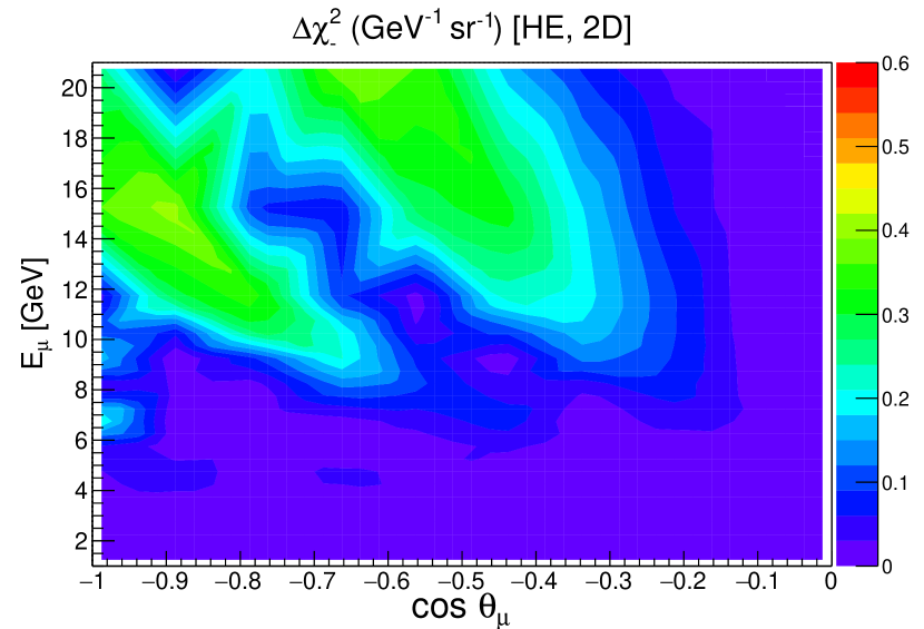
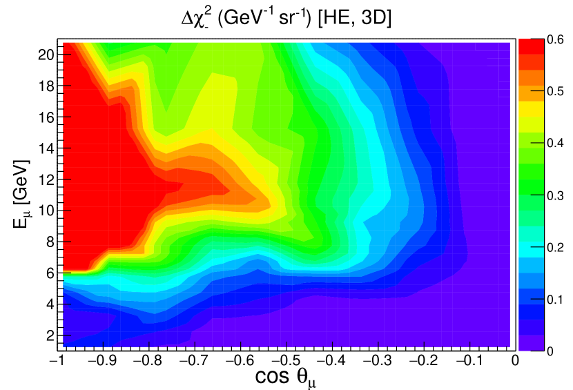
Let us first identify the regions in and plane which give significant contributions towards . In Fig. 4, we show the distribution666In Fig. 4, we do not consider the constant contributions in coming from the term which involves five pull parameters in Eq. 24 and Eq. 26. Also, we do not marginalize over the oscillation parameters in the fit to produce these figures. We adopt the same strategy for Fig. 5 as well. Note that we show our final results considering full pull contributions and marginalizing over the oscillation parameters in the fit as mentioned in previous section. of from events in the reconstructed [-] plane using 500 ktyr exposure of the ICAL detector and assuming NH. In all the panels of Fig. 4, we consider in the fit and show the results for the following four different choices of binning schemes and observables: i) top left panel: [LE, 2D], ii) top right panel: [LE, 3D], iii) bottom left panel: [HE, 2D], iv) bottom right panel: [HE, 3D]. We show the distribution of from events in the plane of reconstructed and for these four different cases in Fig. 5 considering in the fit. In left panels of Figs. 4 and Fig. 5, we show the sensitivity in the plane of reconstructed and for the “2D” analysis, where we do not use any information on hadrons. But, in right panels of these figures, we portray the sensitivity in the plane of reconstructed and for the “3D” case, where the events are further divided into four sub-bins depending on the reconstructed hadron energy for LE (see Table 2) and HE binning schemes (see Table 3).

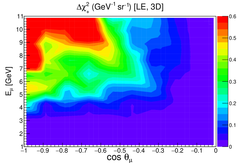
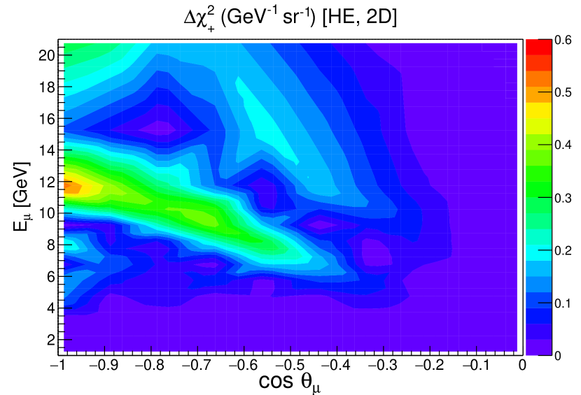
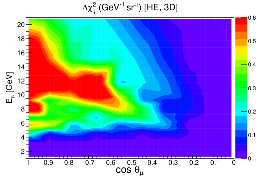
The common features which are emerging from all the panels in Fig. 4 and Fig. 5 are that most of the sensitivity towards the NSI parameter stems from higher energies and longer baselines where the matter effect term 2 becomes sizeable. We observe similar trends in Fig 2 where we plot the differences in oscillation probabilities for the cases and . The event spectra as shown in Fig. 3 also confirm this fact. Fig. 4 and Fig. 5 clearly demonstrate while going from LE to HE binning scheme that the sensitivity towards the NSI parameter get enhanced due to the increment in the range of from 11 GeV to 21 GeV and for extending the fourth bin from 15 GeV to 25 GeV. We can also observe from these figures that with the addition of hadron energy information, the area in the - plane which contributes significantly to increases, consequently enhancing the net for both LE and HE binning schemes. Here, we would like to mention that the increase in is not just due to the information contained in , but also due to the valuable information coming from the correlation between and muon momentum (, ).
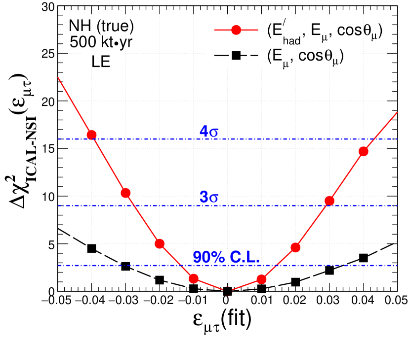
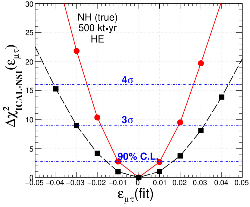
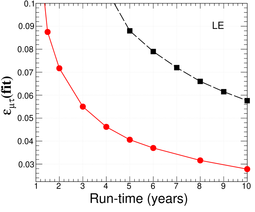
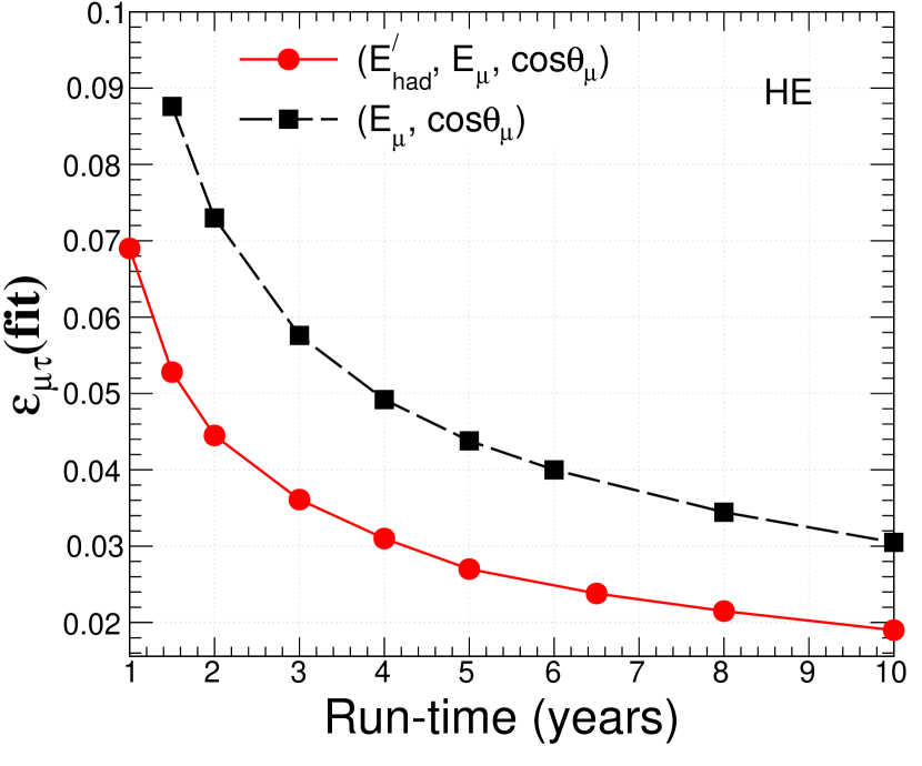
In Fig. 6, we show the sensitivity of the ICAL detector to constrain using an exposure of 500 ktyr and assuming NH as the true mass hierarchy. We obtain these results after performing marginalization over , , and both the choices of mass hierarchy as discussed in Sec. 5.2. In the left (right) panel, the results are shown for the LE (HE) binning scheme. In each panel, the red solid line shows the sensitivity for the “3D” case where we consider , , and as observables. The black dashed line in each panel portrays the sensitivity for the “2D” case considering and as observables. We see considerable improvement in the sensitivity for both the LE and HE binning schemes when we add along with and as observables. We see significant gain in the sensitivity when we increase the range from 11 GeV to 21 GeV and extend the fourth bin from 15 GeV to 25 GeV. It is evident from both the panels in Fig. 6 that for the [HE, 3D] case, we obtain the best sensitivity towards the NSI parameter , whereas the [LE, 2D] mode gives the most conservative limits.
| Observable | Binning scheme | Constraints at 3 (90 C.L.) | |
| NH (true) | IH (true) | ||
| (Eμ, ) | LE | ||
| () | ( ) | ||
| HE | |||
| () | () | ||
| () | LE | ||
| () | () | ||
| HE | |||
| () | () | ||
The 3 (90) confidence level bounds on the flavor violating NSI parameter obtained using 500 ktyr exposure of the ICAL are listed in Table 4. The results are shown for true NH (3rd column) and true IH (4th column). For the [HE, 3D] case, we expect the best limit of at 90 C.L. using 500 ktyr exposure of the ICAL detector and irrespective of the choices of true mass hierarchy. For the [LE, 2D] mode, we obtain the most conservative limit of at 90 confidence level assuming NH as true choice. So far we have considered as our benchmark choice both in data and theory. If we consider the current best fit value of Capozzi:2017ipn ; Esteban:2018azc ; deSalas:2017kay , we have checked that our results will remain almost unaltered. For an instance, if we consider in the fit, then we obtain assuming for the [HE, 3D] mode (see the red curve in the right panel of Fig. 6). Under the same condition, if we take , then the changes to .
6.2 Advantage of having Charge Identification Capability
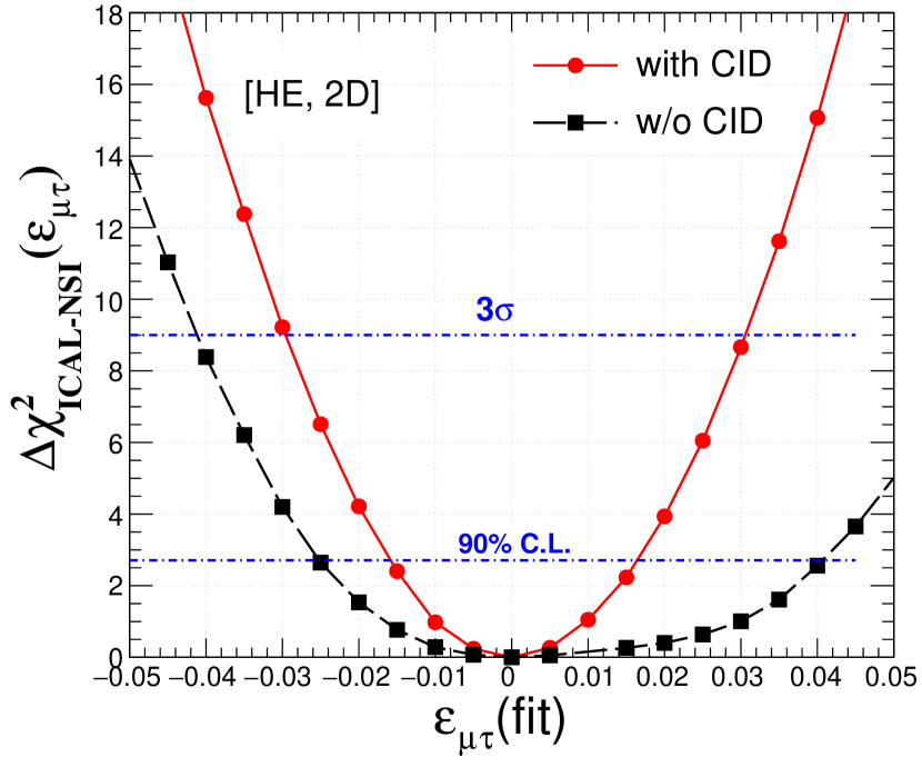
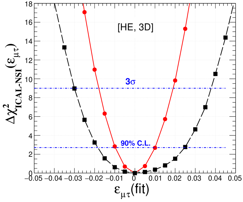
The ICAL detector is expected to have a uniform magnetic field of strength around 1.5 Tesla over the entire detector. It will enable the ICAL detector to identify the and events separately by observing the bending of their tracks in the opposite directions in the presence of the magnetic field. We label this feature of ICAL as the charge identification capability. In Ref. Chatterjee:2014vta , it has been demonstrated that the ICAL detector will have a very good CID efficiency over a wide range of reconstructed and . In this work, we estimate for the first time the gain in the sensitivity that ICAL may have in constraining the NSI parameter due to its CID capability. In each panel of Fig. 7, we show the expected sensitivity of ICAL in constraining with (red solid line) and without (black dashed line) CID capability using 500 ktyr exposure and assuming NH. While preparing these plots, we keep the oscillation parameters fixed in the fit and depict the result for the 2D: , (3D: , , ) mode in the left (right) panel assuming the HE binning scheme. It is apparent from Fig. 7 that the CID capability of ICAL in distinguishing and events plays an important role to make it sensitive to the NSI parameter like the mass hierarchy measurements Devi:2014yaa ; Kumar:2017sdq . In the following, we quote the 90 confidence level limits on that the ICAL detector can place with and without CID capabilities for [HE, 2D] and [HE, 3D] modes. [HE, 2D] mode (left panel of Fig. 7):
| (30) |
[HE, 3D] mode (right panel of Fig. 7):
| (31) |
The limits on mentioned in Eq. 30 and Eq. 31 clearly demonstrate the improvement that the ICAL detector can have in constraining the NSI parameter due its CID capability.
6.3 Limits on for various exposures
Fig. 8 shows the 3 limit on as a function of run-time777Note that while varying run-time in Fig. 8, we always consider the same LE and HE binning schemes as given in Table 2 and Table 3 respectively. For less exposure (small run-time), we may not have sufficient statistics in most of the bins. One needs to consider larger bin widths to tackle this issue which in turn may effect the sensitivity results. We have plans to address this issue in our future study. for 50 kt ICAL. The left (right) panel is for LE (HE) binning scheme. In each panel, the black and red lines depict the results for 2D (, ) and 3D (, , ) modes respectively. In Fig. 8, various sensitivity curves are drawn keeping all the oscillation parameters fixed in the fit and assuming NH. Here, we give the results only for positive values of . We have checked that the results look similar if we consider negative values of as well. If we take total 250 ktyr exposure (50 kt ICAL with a run-time of 5 years), the expected bound is at C.L. assuming NH in [HE, 3D] binning scheme. It suggests that ICAL can place competitive constraints on even for less exposure.
6.4 Impact of non-zero on Mass Hierarchy Determination
This section is devoted to study how the flavor violating NSI parameter affects the mass hierarchy measurement which is the prime goal of the ICAL detector. We quantify the performance ICAL to rule out the wrong hierarchy by adopting the following expression:
| (32) |
Here, we obtain and by performing the fit to the prospective data assuming true and false mass hierarchy respectively. Since the statistical fluctuations are suppressed in our analysis, . First, we estimate the sensitivity of the ICAL detector to determine the neutrino mass hierarchy by adopting the procedure as outlined in Ref. Devi:2014yaa for the standard case, which we denote as “ (SM)” in the third column of Table 5. Next, to estimate the mass hierarchy sensitivity in the presence of non-zero , we adopt the following strategy.
| True MH | Analysis Mode | (SM) | (SM + ) | Reduction |
| LE binning scheme | ||||
| NH | () () | 5.62 8.66 | 4.81 7.49 | 14.4 13.5 |
| IH | () () | 5.31 8.48 | 4.14 6.88 | 22.0 18.9 |
| HE binning scheme | ||||
| NH | () () | 5.96 9.13 | 5.37 8.16 | 9.9 10.6 |
| IH | () () | 5.66 8.99 | 4.95 7.66 | 12.5 14.8 |
We generate the data with a given mass hierarchy assuming . Then, while fitting the prospective data with the opposite hierarchy, we introduce in the fit and marginalize over it in the range of - 0.1 to 0.1 along with the oscillation parameters and in their allowed ranges as mentioned in Sec. 5. We label this result as “ (SM + )” in the fourth column of Table 5. We show our results for various choices of binning schemes and observables assuming both true NH and true IH. We consider 500 ktyr exposure of the ICAL detector. We can see from Table 5 that depending on the choice of true mass hierarchy and the analysis mode, the mass hierarchy sensitivity of ICAL gets reduced by 10 to 20 due to the presence of non-zero in the fit.
6.5 Precision Measurement of Atmospheric Parameters with non-zero
Next, we turn our attention to the precise measurement of atmospheric oscillation parameters and using 500 ktyr exposure of the ICAL detector. We quantify this performance indicator using the following expression:
| (33) |
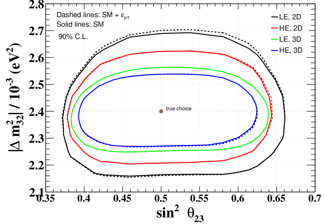
where is the minimum value of in the allowed parameter range. Since we suppress the statistical fluctuations, we have . First, considering (true) = 0.5 and (true) = 2.4 10-3 eV2, we estimate the allowed regions in - (test) plane in the absence of at 90 C.L. (2 d.o.f.). We show these results for the “SM” case using solid lines in Fig. 9 for various analysis modes. For the [HE, 3D] case, we achieve the best precision for the atmospheric parameters, and for the [LE, 2D] case, we have the most conservative results.
Next, we study the impact of non-zero in the precision measurement of atmospheric parameters in the following fashion. We again generate the prospective data considering the true values of and as mentioned above. Then, while estimating the allowed regions in - (test) plane, we introduce in the fit and marginalize over it in the range of [-0.1, 0.1]. We present these results for the “SM + ” case at C.L. (2 d.o.f.) with the help of dashed lines in Fig. 9 for various analysis modes. We do not see any appreciable change in the contours when we introduce in the fit and vary in its 10 range. It suggests that the precision measurement of atmospheric oscillation parameters at the ICAL detector is quite robust even if we marginalize over in the fit. Similar results were obtained by the Super-Kamiokande Collaboration in Ref. Mitsuka:2011ty , where they studied the impact of NSI’s in - sector using their Phase I and Phase II atmospheric data.
7 Summary and Concluding Remarks
In this paper, we explore the possibility of lepton flavor violating neutral current non-standard interactions (NSI’s) of atmospheric neutrino and antineutrino while they travel long distances inside the Earth matter before reaching to the ICAL detector. During the propagation of these neutrinos, we allow an extra interaction vertex with as the incoming particle and as the outgoing one and vice versa. With such an interaction vertex, the neutral current non-standard interaction of neutrino with matter fermions gives rise to a new matter potential whose relative strength as compared to the standard matter potential () is denoted by .
We show that the ICAL detector would be able to place tight constraints on the NSI parameter considering reconstructed hadron energy and muon momentum as observables. We find that with GeV and with [] as observables, the expected limit on at 90 C.L. is . If we increase the muon energy range from 11 to 21 GeV ( GeV) and consider the reconstructed hadron energy () as an extra observable on top of the four momenta of muon (), we find a significant improvement in the limit which is at 90 C.L. using 500 ktyr exposure of the ICAL detector. We observe that the charge identification capability of the ICAL detector plays an important role to obtain these tight constraints on as mentioned above.
Assuming 1 to 21 GeV reconstructed muon energy range and considering and as observables, we find that the mass hierarchy sensitivity at the ICAL detector deteriorates by 10 if we introduce the NSI parameter in the fit and marginalize over it in the range of -0.1 to 0.1 along with other standard oscillation parameters. On the other hand, the precision measurement of atmospheric oscillation parameters at the ICAL detector is quite robust even if we marginalize over the NSI parameter in fit in the range -0.1 to 0.1.
8 Acknowledgment
The INO-ICAL Collaboration is exploring various physics potentials of the proposed ICAL detector and this work is a part of that ongoing effort. This work would not have been possible without the contribution of several members of the Collaboration. We would like to thank A. Dighe, A.M. Srivastava, P. Agrawal, S. Goswami, D. Indumathi, S. Choubey, S. Uma Sankar for their useful comments on our work. We thank N. Mondal, A. Dighe, and S. Goswami for helping us during the INO Internal Review Process. A.K. acknowledges the support from the Department of Atomic Energy (DAE), Government of India. S.K.A. acknowledges the support from DST/INSPIRE Research Grant [IFA-PH-12], Department of Science and Technology, India and the Young Scientist Project [INSA/SP/YSP/144/2017/1578] from the Indian National Science Academy. T. T. acknowledges support from the Ministerio de Economíay Competitividad (MINECO): Plan Estatal de Investigación (ref. FPA2015- 65150-C3-1-P, MINECO/FEDER), Severo Ochoa Centre of Excellence and MultiDark Consolider (MINECO), and Prometeo program (Generalitat Valenciana), Spain.
References
- (1) Particle Data Group Collaboration, C. Patrignani et al., Review of Particle Physics, Chin. Phys. C40 (2016), no. 10 100001.
- (2) F. Capozzi, E. Di Valentino, E. Lisi, A. Marrone, A. Melchiorri, and A. Palazzo, Global constraints on absolute neutrino masses and their ordering, Phys. Rev. D95 (2017), no. 9 096014, [arXiv:1703.04471].
- (3) I. Esteban, M. C. Gonzalez-Garcia, A. Hernandez-Cabezudo, M. Maltoni, and T. Schwetz, Global analysis of three-flavour neutrino oscillations: synergies and tensions in the determination of , and the mass ordering, arXiv:1811.05487.
- (4) P. F. de Salas, D. V. Forero, C. A. Ternes, M. Tortola, and J. W. F. Valle, Status of neutrino oscillations 2018: 3 hint for normal mass ordering and improved CP sensitivity, Phys. Lett. B782 (2018) 633–640, [arXiv:1708.01186].
- (5) M. C. Gonzalez-Garcia, M. M. Guzzo, P. I. Krastev, H. Nunokawa, O. L. G. Peres, V. Pleitez, J. W. F. Valle, and R. Zukanovich Funchal, Atmospheric neutrino observations and flavor changing interactions, Phys. Rev. Lett. 82 (1999) 3202–3205, [hep-ph/9809531].
- (6) S. Bergmann and A. Kagan, Z - induced FCNCs and their effects on neutrino oscillations, Nucl. Phys. B538 (1999) 368–386, [hep-ph/9803305].
- (7) S. Bergmann, Y. Grossman, and E. Nardi, Neutrino propagation in matter with general interactions, Phys. Rev. D60 (1999) 093008, [hep-ph/9903517].
- (8) P. Lipari and M. Lusignoli, On exotic solutions of the atmospheric neutrino problem, Phys. Rev. D60 (1999) 013003, [hep-ph/9901350].
- (9) M. M. Guzzo, H. Nunokawa, P. C. de Holanda, and O. L. G. Peres, On the massless ’just-so’ solution to the solar neutrino problem, Phys. Rev. D64 (2001) 097301, [hep-ph/0012089].
- (10) M. C. Gonzalez-Garcia, Y. Grossman, A. Gusso, and Y. Nir, New CP violation in neutrino oscillations, Phys. Rev. D64 (2001) 096006, [hep-ph/0105159].
- (11) A. M. Gago, M. M. Guzzo, H. Nunokawa, W. J. C. Teves, and R. Zukanovich Funchal, Probing flavor changing neutrino interactions using neutrino beams from a muon storage ring, Phys. Rev. D64 (2001) 073003, [hep-ph/0105196].
- (12) Z. Berezhiani and A. Rossi, Limits on the nonstandard interactions of neutrinos from e+ e- colliders, Phys. Lett. B535 (2002) 207–218, [hep-ph/0111137].
- (13) P. Huber and J. W. F. Valle, Nonstandard interactions: Atmospheric versus neutrino factory experiments, Phys. Lett. B523 (2001) 151–160, [hep-ph/0108193].
- (14) N. Fornengo, M. Maltoni, R. Tomas, and J. W. F. Valle, Probing neutrino nonstandard interactions with atmospheric neutrino data, Phys. Rev. D65 (2002) 013010, [hep-ph/0108043].
- (15) P. Huber, T. Schwetz, and J. W. F. Valle, Confusing nonstandard neutrino interactions with oscillations at a neutrino factory, Phys. Rev. D66 (2002) 013006, [hep-ph/0202048].
- (16) A. M. Gago, M. M. Guzzo, P. C. de Holanda, H. Nunokawa, O. L. G. Peres, V. Pleitez, and R. Zukanovich Funchal, Global analysis of the postSNO solar neutrino data for standard and nonstandard oscillation mechanisms, Phys. Rev. D65 (2002) 073012, [hep-ph/0112060].
- (17) Z. Berezhiani, R. S. Raghavan, and A. Rossi, Probing nonstandard couplings of neutrinos at the Borexino detector, Nucl. Phys. B638 (2002) 62–80, [hep-ph/0111138].
- (18) T. Ota, J. Sato, and N.-a. Yamashita, Oscillation enhanced search for new interaction with neutrinos, Phys. Rev. D65 (2002) 093015, [hep-ph/0112329].
- (19) S. Davidson, C. Pena-Garay, N. Rius, and A. Santamaria, Present and future bounds on nonstandard neutrino interactions, JHEP 03 (2003) 011, [hep-ph/0302093].
- (20) A. Friedland, C. Lunardini, and M. Maltoni, Atmospheric neutrinos as probes of neutrino-matter interactions, Phys. Rev. D70 (2004) 111301, [hep-ph/0408264].
- (21) M. C. Gonzalez-Garcia and M. Maltoni, Atmospheric neutrino oscillations and new physics, Phys. Rev. D70 (2004) 033010, [hep-ph/0404085].
- (22) M. M. Guzzo, P. C. de Holanda, and O. L. G. Peres, Effects of nonstandard neutrino interactions on MSW - LMA solution to the solar neutrino problems, Phys. Lett. B591 (2004) 1–6, [hep-ph/0403134].
- (23) A. Friedland and C. Lunardini, A Test of tau neutrino interactions with atmospheric neutrinos and K2K, Phys. Rev. D72 (2005) 053009, [hep-ph/0506143].
- (24) N. Kitazawa, H. Sugiyama, and O. Yasuda, Will MINOS see new physics?, hep-ph/0606013.
- (25) G. Mangano, G. Miele, S. Pastor, T. Pinto, O. Pisanti, and P. D. Serpico, Effects of non-standard neutrino-electron interactions on relic neutrino decoupling, Nucl. Phys. B756 (2006) 100–116, [hep-ph/0607267].
- (26) M. Blennow, T. Ohlsson, and W. Winter, Non-standard Hamiltonian effects on neutrino oscillations, Eur. Phys. J. C49 (2007) 1023–1039, [hep-ph/0508175].
- (27) A. Esteban-Pretel, R. Tomas, and J. W. F. Valle, Probing non-standard neutrino interactions with supernova neutrinos, Phys. Rev. D76 (2007) 053001, [arXiv:0704.0032].
- (28) J. Barranco, O. G. Miranda, and T. I. Rashba, Low energy neutrino experiments sensitivity to physics beyond the Standard Model, Phys. Rev. D76 (2007) 073008, [hep-ph/0702175].
- (29) N. C. Ribeiro, H. Minakata, H. Nunokawa, S. Uchinami, and R. Zukanovich-Funchal, Probing Non-Standard Neutrino Interactions with Neutrino Factories, JHEP 12 (2007) 002, [arXiv:0709.1980].
- (30) J. Kopp, M. Lindner, and T. Ota, Discovery reach for non-standard interactions in a neutrino factory, Phys. Rev. D76 (2007) 013001, [hep-ph/0702269].
- (31) M. Blennow, D. Meloni, T. Ohlsson, F. Terranova, and M. Westerberg, Non-standard interactions using the OPERA experiment, Eur. Phys. J. C56 (2008) 529–536, [arXiv:0804.2744].
- (32) A. Esteban-Pretel, J. W. F. Valle, and P. Huber, Can OPERA help in constraining neutrino non-standard interactions?, Phys. Lett. B668 (2008) 197–201, [arXiv:0803.1790].
- (33) J. Barranco, O. G. Miranda, C. A. Moura, and J. W. F. Valle, Constraining non-standard neutrino-electron interactions, Phys. Rev. D77 (2008) 093014, [arXiv:0711.0698].
- (34) J. Kopp, M. Lindner, T. Ota, and J. Sato, Non-standard neutrino interactions in reactor and superbeam experiments, Phys. Rev. D77 (2008) 013007, [arXiv:0708.0152].
- (35) M. Blennow, T. Ohlsson, and J. Skrotzki, Effects of non-standard interactions in the MINOS experiment, Phys. Lett. B660 (2008) 522–528, [hep-ph/0702059].
- (36) T. Ohlsson and H. Zhang, Non-Standard Interaction Effects at Reactor Neutrino Experiments, Phys. Lett. B671 (2009) 99–104, [arXiv:0809.4835].
- (37) M. B. Gavela, D. Hernandez, T. Ota, and W. Winter, Large gauge invariant non-standard neutrino interactions, Phys. Rev. D79 (2009) 013007, [arXiv:0809.3451].
- (38) A. Bolanos, O. G. Miranda, A. Palazzo, M. A. Tortola, and J. W. F. Valle, Probing non-standard neutrino-electron interactions with solar and reactor neutrinos, Phys. Rev. D79 (2009) 113012, [arXiv:0812.4417].
- (39) S. Antusch, J. P. Baumann, and E. Fernandez-Martinez, Non-Standard Neutrino Interactions with Matter from Physics Beyond the Standard Model, Nucl. Phys. B810 (2009) 369–388, [arXiv:0807.1003].
- (40) C. Biggio, M. Blennow, and E. Fernandez-Martinez, General bounds on non-standard neutrino interactions, JHEP 08 (2009) 090, [arXiv:0907.0097].
- (41) F. J. Escrihuela, O. G. Miranda, M. A. Tortola, and J. W. F. Valle, Constraining nonstandard neutrino-quark interactions with solar, reactor and accelerator data, Phys. Rev. D80 (2009) 105009, [arXiv:0907.2630]. [Erratum: Phys. Rev.D80,129908(2009)].
- (42) A. M. Gago, H. Minakata, H. Nunokawa, S. Uchinami, and R. Zukanovich Funchal, Resolving CP Violation by Standard and Nonstandard Interactions and Parameter Degeneracy in Neutrino Oscillations, JHEP 01 (2010) 049, [arXiv:0904.3360].
- (43) C. Biggio, M. Blennow, and E. Fernandez-Martinez, Loop bounds on non-standard neutrino interactions, JHEP 03 (2009) 139, [arXiv:0902.0607].
- (44) H. Oki and O. Yasuda, Sensitivity of the T2KK experiment to the non-standard interaction in propagation, Phys. Rev. D82 (2010) 073009, [arXiv:1003.5554].
- (45) J. Kopp, P. A. N. Machado, and S. J. Parke, Interpretation of MINOS data in terms of non-standard neutrino interactions, Phys. Rev. D82 (2010) 113002, [arXiv:1009.0014].
- (46) D. V. Forero and M. M. Guzzo, Constraining nonstandard neutrino interactions with electrons, Phys. Rev. D84 (2011) 013002.
- (47) F. J. Escrihuela, M. Tortola, J. W. F. Valle, and O. G. Miranda, Global constraints on muon-neutrino non-standard interactions, Phys. Rev. D83 (2011) 093002, [arXiv:1103.1366].
- (48) M. Gonzalez-Garcia, M. Maltoni, and J. Salvado, Testing matter effects in propagation of atmospheric and long-baseline neutrinos, JHEP 1105 (2011) 075, [arXiv:1103.4365].
- (49) P. Coloma, A. Donini, J. Lopez-Pavon, and H. Minakata, Non-Standard Interactions at a Neutrino Factory: Correlations and CP violation, JHEP 08 (2011) 036, [arXiv:1105.5936].
- (50) R. Adhikari, S. Chakraborty, A. Dasgupta, and S. Roy, Non-standard interaction in neutrino oscillations and recent Daya Bay, T2K experiments, Phys. Rev. D86 (2012) 073010, [arXiv:1201.3047].
- (51) S. K. Agarwalla, F. Lombardi, and T. Takeuchi, Constraining Non-Standard Interactions of the Neutrino with Borexino, JHEP 12 (2012) 079, [arXiv:1207.3492].
- (52) M. C. Gonzalez-Garcia and M. Maltoni, Determination of matter potential from global analysis of neutrino oscillation data, JHEP 09 (2013) 152, [arXiv:1307.3092].
- (53) T. Ohlsson, H. Zhang, and S. Zhou, Effects of nonstandard neutrino interactions at PINGU, Phys. Rev. D88 (2013), no. 1 013001, [arXiv:1303.6130].
- (54) T. Ohlsson, Status of non-standard neutrino interactions, Rept. Prog. Phys. 76 (2013) 044201, [arXiv:1209.2710].
- (55) S. Choubey, A. Ghosh, T. Ohlsson, and D. Tiwari, Neutrino Physics with Non-Standard Interactions at INO, JHEP 12 (2015) 126, [arXiv:1507.02211].
- (56) Y. Farzan and M. Tortola, Neutrino oscillations and Non-Standard Interactions, Front.in Phys. 6 (2018) 10, [arXiv:1710.09360].
- (57) O. G. Miranda and H. Nunokawa, Non standard neutrino interactions: current status and future prospects, New J. Phys. 17 (2015), no. 9 095002, [arXiv:1505.06254].
- (58) L. Wolfenstein, Neutrino Oscillations in Matter, Phys.Rev. D17 (1978) 2369–2374.
- (59) Super-Kamiokande Collaboration, G. Mitsuka et al., Study of Non-Standard Neutrino Interactions with Atmospheric Neutrino Data in Super-Kamiokande I and II, Phys.Rev. D84 (2011) 113008, [arXiv:1109.1889].
- (60) J. Salvado, O. Mena, S. Palomares-Ruiz, and N. Rius, Non-standard interactions with high-energy atmospheric neutrinos at IceCube, arXiv:1609.03450.
- (61) IceCube Collaboration, M. Aartsen et al., Search for Nonstandard Neutrino Interactions with IceCube DeepCore, Phys. Rev. D97 (2018), no. 7 072009, [arXiv:1709.07079].
- (62) A. Dziewonski and D. Anderson, Preliminary reference earth model, Phys.Earth Planet.Interiors 25 (1981) 297–356.
- (63) H. Nunokawa, S. J. Parke, and R. Zukanovich Funchal, Another possible way to determine the neutrino mass hierarchy, Phys.Rev. D72 (2005) 013009, [hep-ph/0503283].
- (64) A. de Gouvea, J. Jenkins, and B. Kayser, Neutrino mass hierarchy, vacuum oscillations, and vanishing —U(e3)—, Phys. Rev. D71 (2005) 113009, [hep-ph/0503079].
- (65) D. Hollander and I. Mocioiu, Sterile neutrinos at LBNE, arXiv:1408.1749.
- (66) ICAL Collaboration, S. Ahmed et al., Physics Potential of the ICAL detector at the India-based Neutrino Observatory (INO), Pramana 88 (2017), no. 5 79, [arXiv:1505.07380].
- (67) D. Casper, The Nuance neutrino physics simulation, and the future, Nucl.Phys.Proc.Suppl. 112 (2002) 161–170, [hep-ph/0208030].
- (68) M. Sajjad Athar, M. Honda, T. Kajita, K. Kasahara, and S. Midorikawa, Atmospheric neutrino flux at INO, South Pole and Pyhásalmi, Phys.Lett. B718 (2013) 1375–1380, [arXiv:1210.5154].
- (69) M. Honda, M. S. Athar, T. Kajita, K. Kasahara, and S. Midorikawa, Atmospheric neutrino flux calculation using the NRLMSISE-00 atmospheric model, Phys. Rev. D92 (2015), no. 2 023004, [arXiv:1502.03916].
- (70) M. Honda, T. Kajita, K. Kasahara, and S. Midorikawa, Improvement of low energy atmospheric neutrino flux calculation using the JAM nuclear interaction model, Phys.Rev. D83 (2011) 123001, [arXiv:1102.2688].
- (71) A. Chatterjee, K. Meghna, K. Rawat, T. Thakore, V. Bhatnagar, et al., A Simulations Study of the Muon Response of the Iron Calorimeter Detector at the India-based Neutrino Observatory, JINST 9 (2014) P07001, [arXiv:1405.7243].
- (72) M. M. Devi, A. Ghosh, D. Kaur, L. S. Mohan, S. Choubey, et al., Hadron energy response of the Iron Calorimeter detector at the India-based Neutrino Observatory, JINST 8 (2013) P11003, [arXiv:1304.5115].
- (73) M. Blennow, P. Coloma, P. Huber, and T. Schwetz, Quantifying the sensitivity of oscillation experiments to the neutrino mass ordering, JHEP 1403 (2014) 028, [arXiv:1311.1822].
- (74) M. M. Devi, T. Thakore, S. K. Agarwalla, and A. Dighe, Enhancing sensitivity to neutrino parameters at INO combining muon and hadron information, JHEP 1410 (2014) 189, [arXiv:1406.3689].
- (75) A. Ghosh, T. Thakore, and S. Choubey, Determining the Neutrino Mass Hierarchy with INO, T2K, NOvA and Reactor Experiments, JHEP 1304 (2013) 009, [arXiv:1212.1305].
- (76) P. Huber, M. Lindner, and W. Winter, Superbeams versus neutrino factories, Nucl.Phys. B645 (2002) 3–48, [hep-ph/0204352].
- (77) G. Fogli, E. Lisi, A. Marrone, D. Montanino, and A. Palazzo, Getting the most from the statistical analysis of solar neutrino oscillations, Phys.Rev. D66 (2002) 053010, [hep-ph/0206162].