Unified Description of Multiplicity Distributions and Bose-Einstein Correlations at the LHC Based on the Three-Negative Binomial Distribution

Abstract

Using the Monte Carlo data at 7 TeV collected by the ATLAS collaboration (PYTHIA 6), we examine the necessity of applying the three-negative binomial distribution (T-NBD). By making use of the T-NBD formulation, we analyze the multiplicity distribution (MD) and the Bose-Einstein correlation (BEC) at the Large Hadron Collider (LHC). In the T-NBD framework, the BEC is expressed by two degrees of coherence $\lambda_{1}$ and $\lambda_{2}$ and two kinds of exchange functions $E_{1}^{2}$ and $E_{2}^{2}$ that act over interaction ranges $R_{1}$ and $R_{2}$, respectively. Using the calculated $\lambda_{1}$ and $\lambda_{2}$ based on the T-NBD, along with free $\lambda_{1}$ and $\lambda_{2}$, we analyze the BEC data at 0.9 and 7 TeV. The estimated parameters $R_{1}$ and $R_{2}$ are almost coincident and seem to be consistent with $pp$ collisions. We also present an enlarged Koba-Nielsen-Olesen (KNO) scaling function based on the T-NBD, and apply it to KNO scaling at LHC energies. The enlarged scaling function describes the observed violation of the KNO scaling.

1 Introduction

1.1 Negative Binomial Distribution (NBD)

Approximately three decades ago, the UA5 collaboration [1] discovered a violation of Koba-Nielsen-Olesen (KNO) scaling [2] at CERN S$\bar{p}p$S collider. To explain those data, the UA5 collaboration assumed a double-negative binomial distribution (D-NBD) of the data. The NBD is given as

$$P_{\rm NBD}(n,\,k,\,\langle n\rangle)=\frac{\Gamma(n+k)}{\Gamma(n+1)\Gamma(k)}\frac{(\langle n\rangle/k)^{n}}{(1+\langle n\rangle/k)^{n+k}},$$ (1)

where $\langle n\rangle$ and $k$ are the averaged multiplicity and the intrinsic parameter of the NBD, respectively. The D-NBD is expressed as

$$P_{\rm(D\mathchar 45\relax N)}(n,\,\langle n\rangle,\,\alpha_{i},\,k_{i})=\sum_{i=1}^{2}\alpha_{i}P_{{\rm NBD}_{i}}(n,\,\langle n_{i}\rangle,\,k_{i}),$$ (2)

where $\alpha_{1}+\alpha_{2}=1$. Using Eqs. (1) and (2), several authors [3, 4, 5, 6] have analyzed the multiplicity distribution (MD) of data at high energies, such as the high-energy data of the Large Hadron Collider (LHC) [7, 8]. Among those analyses, the three-NBD (T-NBD) was applied by Zborovsky [9]:

$$P_{\rm(T\mathchar 45\relax N)}(n,\,\langle n\rangle,\,\alpha_{i},\,k_{i})=\sum_{i=1}^{3}\alpha_{i}P_{{\rm NBD}_{i}}(n,\,\langle n_{i}\rangle,\,k_{i}).$$ (3)

where $\alpha_{1}+\alpha_{2}+\alpha_{3}=1.0$ (see also [6]).

Here, we address the question “Why must the MD of LHC data be analyzed in the T-NBD framework?” To find a plausible answer, we must consider the constraints adopted by the ATLAS and CMS collaborations (for example, $|\eta|<2.5$ and $|\eta|<2.4$). Even in restricted $\eta$ regions, Monte Carlo (MC) estimations have revealed that three processes, i.e., the non-diffractive dissociation (ND), the single-diffractive dissociation (SD), and the double-diffractive dissociation (DD) contribute to the MD at LHC energies [10, 11, 12].

For the reader’s convenience, our analysis results of MC data at 7 TeV collected by the ATLAS collaboration are presented in Tables 11 and 12, and Figs. 5 and 6 of Appendix A. The individual data ensembles of ND, SD, and DD, defined by the partial probability distributions $P_{\rm ND}(n)$, $P_{\rm SD}(n)$, and $P_{\rm DD}(n)$ respectively, are reasonably described by the D-NBD (see Table 1). Accordingly, the total probability $P_{\rm tot}=P_{\rm ND}+P_{\rm SD}+P_{\rm DD}$ is also described by the T-NBD. This behavior implies an important role for the T-NBD in MD analyses at LHC energies.

Table 1: Stochastic properties of the three ensembles computed by PYTHIA 8 in the ATLAS experiment at 7 TeV (see Figs. 5 and 6 in Appendix A).

QCD	acceptance and	stochastic property	stochastic description
PYTHIA 6	correction by	of individual ensemble	of sum of three ensembles
7 TeV	ATLAS coll. [10]
ND	$P_{\rm ND}(n)$	(sum of)
	$f_{\rm ND}=\sum P_{\rm ND}(n)=0.787$	NBD1 and NBD2	T-NBD Eq. (3)
SD	$P_{\rm SD}(n)$		$P_{\rm(T\mathchar 45\relax N)}(n,\,\langle n\rangle,\,\alpha_{i},\,k_{i})=\hskip 14.22636pt$
	$f_{\rm SD}=0.121$	NBD2 and NBD3	$\sum_{i=1}^{3}\alpha_{i}P_{{\rm NBD}_{i}}(n,\,\langle n_{i}\rangle,\,k_{i})$
DD	$P_{\rm DD}(n)$
	$f_{\rm DD}=0.092$	NBD3 and NBD2
	sum of fractions:	NBDi’s are specified	Eq. (3) is a
	$f_{\rm ND}+f_{\rm SD}+f_{\rm DD}=1.0$	by $(\langle n\rangle,\,k)$	possible candidate

Very recently, Zborovsky [13] revealed the stochastic structure of the T-NBD studying the oscillations in combinations of T-NBDs. As pointed out by Wilk and Wlodarczyk [14], Zborovsky’s work supports the theoretical plausibility of the T-NBD. See also recent study on this subject [15]. Regarding recent T-NBD investigations, we approach the T-NBD from a different perspective, namely, the identical particle effect [16, 17, 18] observed at the LHC (see Refs. [19, 20, 21] and [22, 23, 24] for related theoretical and empirical studies, respectively).

1.2 Bose-Einstein correlation at the LHC

The moments of a charged-particle distributions are calculated as

$$\langle n\rangle = \sum_{i=1}^{3}\alpha_{i}\langle n_{i}\rangle,$$

$$\langle n(n-1)\rangle = \sum_{i=1}^{3}\alpha_{i}\langle n_{i}(n_{i}-1)\rangle=\sum_{i=1}^{3}\alpha_{i}\langle n_{i}\rangle^{2}\left(1.0+\frac{1.0}{k_{i}}\right),$$

$$\langle n(n-1)(n-2\rangle = \sum_{i=1}^{3}\alpha_{i}\langle n_{i}(n_{i}-1)(n_{i}-2)\rangle=\sum_{i=1}^{3}\alpha_{i}\langle n_{i}\rangle^{3}\left(1.0+\frac{3.0}{k_{i}}+\frac{2.0}{k_{i}^{2}}\right).$$ (4)

When the particles are identical, we obtain the following relation (where the charge sign $a$ is $+$ or $-$):

$$\langle n^{a}(n^{a}-1)\rangle=\sum_{i=1}^{3}\alpha_{i}\langle n_{i}^{a}\rangle^{2}\left(1.0+\frac{2.0}{k_{i}}\right),$$ (5)

Eq. (5) can be interpreted as

$${\rm Eq.\ }(\ref{eq5}): \sum_{i=1}^{3}(\mbox{The number of pairs of identical charged particle in MD($P(n)$) with $\alpha_{i}$})$$

$$\qquad\times(\mbox{identical particle effect in MD}).$$

Meanwhile, the authors of [20] recently studied the interrelation between the MD and the Bose-Einstein correlation (BEC) under the D-NBD assumption. To extend the framework of T-NBD, we compute $N^{\rm BG}$ as a function of $\{\alpha_{i},\,\langle n_{i}\rangle:\,i=1\sim 3\}$ (see Ref. [21]). The BEC in the extended framework is given by

$$\frac{N^{\rm(2+:\,2-)}}{N^{\rm BG}}=\dfrac{\sum_{i=1}^{3}\alpha_{i}(\langle n_{i}^{+}\rangle^{2}+\langle n_{i}^{-}\rangle^{2})\left(1.0+\frac{2.0}{k_{i}}\right)}{\sum_{i=0}^{3}2\times(\mbox{The number of pairs of different charged particles $(+-)$ in MD with $\alpha_{i}$})}.$$ (6)

To simplify the calculations, we denote $\langle n_{i}^{+}\rangle=\langle n_{i}^{-}\rangle=\langle n_{i}\rangle/2$. In the denominator $N^{\rm BG}$ of Eq. (6), the three coefficients $\alpha_{i}\langle n_{i}\rangle^{2}$ are given by

$$N^{\rm BG} = \sum_{i=1}^{3}\alpha_{i}\langle n_{i}\rangle^{2}=a_{1}+a_{2}+a_{3}=s,$$ (7)

$$\sum_{i=1}^{3}\left(\frac{a_{i}}{s}\right)=1.$$

In the framework of the T-NBD assumption, we have

$$\frac{N^{\rm(2+:\,2-)}}{N^{\rm BG}}=\sum_{i=1}^{3}\left(\frac{a_{i}}{s}\right)\left(1.0+\frac{2}{k_{i}}E_{{\rm BEC}_{i}}^{2}\right)$$ (8)

To describe the BEC in the $0\leq Q\leq 2$ GeV region, we assume the following exchange function $E_{\rm BEC}^{2}$

$$E_{\rm BEC}^{2}=\ \left\{\begin{array}[]{l}\exp(-RQ)\mbox{ (Exponential function) (E)},\vskip 6.0pt plus 2.0pt minus 2.0pt\\ \exp(-(RQ)^{2})\mbox{ (Gaussian distribution) (G)},\end{array}\right.$$ (11)

where $R$ and $Q$ are the interaction range and the momentum-transfer squared function, respectively. The latter is calculated as $Q=\sqrt{-(p_{1}-p_{2})^{2}}$, where $p_{1}$ and $p_{2}$ are momenta of identical particles.

By making use of those calculations mentioned above, the BEC is then formulated as

$${\rm BEC}_{\rm(T\mathchar 45\relax N)} = 1.0+\sum_{i=1}^{3}\left(\frac{a_{i}}{s}\right)\left(\frac{2}{k_{i}}\right)E_{{\rm BEC}_{i}}^{2}$$ (12)

$$= 1.0+\lambda_{1}^{\rm(T\mathchar 45\relax N)}E_{\rm BEC_{1}}^{2}+\lambda_{2}^{\rm(T\mathchar 45\relax N)}E_{\rm BEC_{2}}^{2}+\mathcal{O}(10^{-3}),$$

where $\lambda_{i}^{\rm(T\mathchar 45\relax N)}=(a_{i}/s)(2/k_{i})$ ($i=1,\,2$). It should be noted that the third component (with coefficient $\alpha_{3}$) exhibits a Poisson property. Because the $k_{3}$ values are large, the third term ($i=3$) does not numerically contribute to BEC_(T-N).

In our BEC analysis of LHC data, we note that all three collaborations (ATLAS, CMS, and LHCb [22, 23, 24]) applied the well-known conventional formula

$${\rm CF_{I}}=1.0+\lambda E_{\rm BEC}^{2},$$ (13)

Regarding Eq. (12) as another conventional formula, we would like to propose that

$${\rm CF_{II}}=1.0+\lambda_{1}^{\rm(II)}E_{\rm BEC_{1}}^{2}+\lambda_{2}^{\rm(II)}E_{\rm BEC_{2}}^{2},$$ (14)

where $\lambda_{1}^{\rm(II)}$ and $\lambda_{2}^{\rm(II)}$ are free parameters. By analyzing the BEC data, we can compare $\lambda_{1}^{\rm(II)}$ and $\lambda_{2}^{\rm(II)}$ in Eq. (14) with the terms $\lambda_{i}^{\rm(T\mathchar 45\relax N)}=(a_{i}/s)(2/k_{i})$ ($i=1,\,2$) in Eq. (12), and the terms $R_{i}^{\rm(T\mathchar 45\relax N)}$ and $R_{i}^{\rm(II)}$ in Eqs. (12) and (14).

The second section of this paper analyzes the MD at 0.9 and 7 TeV through Eq. (3). The second and third moments, and $a_{i}$’s and $(a_{i}/s)(2/k_{i})$’s are displayed in this section. Section 3 analyzes the BEC through Eqs. (12), (13) and (14). This paper concludes with remarks and discussions in Section 4. The appendices analyze the MC data at 7 TeV collected by the ATLAS collaboration (Appendix A) and the KNO scaling data by an enlarged KNO scaling function based on the T-NBD assumption (Appendix B).

2 Multiplicity Distribution ($P(n)$) Analysis

We begin by analyzing the MD at 0.9 TeV and 7 TeV obtained by the ATLAS [7] and CMS [8] collaborations under the T-NBD assumption. The MINUIT program is initialized by assigning random variables to the physical quantities. The estimated parameters are displayed in Fig. 1 and Table 2. Note that both collaborations obtained similar minimum $\chi^{2}$ values at 0.9 TeV. To compare our results with those of Zborovsky [9], we adopt the same treatments to the probability distributions. Specifically, we renormalize Eq. (3) without the $P(0)$ and $P(1)$ as the MD obtained by the ATLAS collaboration, and also renormalize the MD obtained by the CMS collaboration after excluding $P(0)$.

Figure 1: Analysis of MD ($P(n)$) data collected by the ATLAS and CMS collaborations. The $P(n)$ data were computed by Eq. (3). As done in Ref. [9], we exclude $P(0)$ obtained by the CMS in our analysis. All data are renormalized.

Table 2: Analysis (by Eq. (3)) of the MD ($P(n)$) data at 0.9 and 7.0 TeV collected by the ATLAS and CMS collaborations.

	$i$	$\alpha_{i}$	$\langle n_{i}\rangle$	$a_{i}$	$k_{i}$
ATLAS	1	0.640$\pm$0.199	13.493$\pm$2.546	116.519$\pm$56.975	1.78$\pm$0.20
0.9 TeV	2	0.250$\pm$0.164	28.488$\pm$3.588	202.892$\pm$142.572	5.01$\pm$1.37
$\chi^{2}=5.317$	3	0.111$\pm$0.047	10.998$\pm$0.237	13.426$\pm$5.714	28.1$\pm$24.4
ATLAS	1	0.737$\pm$0.053	21.934$\pm$2.392	354.571$\pm$81.430	1.50$\pm$0.08
7.0 TeV	2	0.183$\pm$0.061	57.214$\pm$2.597	599.040$\pm$206.953	5.67$\pm$0.76
$\chi^{2}=5.964$	3	0.080$\pm$0.010	11.164$\pm$0.169	9.971$\pm$1.282	23.4$\pm$8.4
ATLAS	1	0.754$\pm$0.063	22.625$\pm$2.549	385.966$\pm$92.755	1.48$\pm$0.08
7.0 TeV	2	0.164$\pm$0.063	57.936$\pm$2.618	550.479$\pm$217.238	5.94$\pm$0.98
$\chi^{2}=6.160$	3	0.082$\pm$0.010	11.177$\pm$0.178	10.244$\pm$1.291	23.4$\pm$8.7
CMS	1	0.743$\pm$0.179	15.852$\pm$2.454	186.705$\pm$73.245	2.08$\pm$0.20
0.9 TeV	2	0.189$\pm$0.170	32.160$\pm$4.567	195.476$\pm$184.382	6.56$\pm$2.85
$\chi^{2}=4.289$	3	0.068$\pm$0.032	11.624$\pm$0.814	9.188$\pm$4.511	896$\pm$817
CMS	1	0.739$\pm$0.200	15.830$\pm$2.841	185.092$\pm$83.177	2.10$\pm$0.21
0.9 TeV	2	0.193$\pm$0.179	32.093$\pm$5.002	199.236$\pm$194.669	6.49$\pm$3.03
$\chi^{2}=4.941$	3	0.068$\pm$0.031	11.618$\pm$0.810	9.177$\pm$4.384	$\infty$
CMS	1	0.826$\pm$0.091	28.613$\pm$4.126	676.108$\pm$208.928	1.66$\pm$0.12
7.0 TeV	2	0.103$\pm$0.098	67.206$\pm$6.727	465.270$\pm$452.384	6.67$\pm$2.92
$\chi^{2}=2.275$	3	0.071$\pm$0.028	13.018$\pm$0.870	12.036$\pm$5.012	38.1$\pm$73.6

Table 3: Second and third moments of MD at 0.9 TeV and 7 TeV, measured (data) and calculated by Eqs. (2) (D-NBD) and (3) (T-NBD).

	$\langle n(n-1)\rangle$ ($\times 10^{3}$)			$\langle n(n-1)(n-2)\rangle$ ($\times 10^{4}$)
	data	D-NBD	T-NBD	data	D-NBD	T-NBD
ATLAS 0.9 TeV	0.454$\pm$0.026	0.450	0.439	1.55$\pm$0.13	1.54	1.53
ATLAS 7.0 TeV	1.35$\pm$0.08	1.35	1.30	8.75$\pm$0.79	9.09	8.43
CMS 0.9 TeV	0.488$\pm$0.050	0.525	0.511	1.73$\pm$0.22	1.86	1.82
CMS 7.0 TeV	1.57$\pm$0.13	1.67	1.63	10.94$\pm$1.10	11.89	11.52

Our results in Table 2 almost match those of Zborovsky [9]. Moreover, the empirical values of the second and third moments almost equal those of the D-NBD and T-NBD (Table 3). From the values in Table 2, we obtain $\lambda_{i}^{\rm(T\mathchar 45\relax N)}=(\alpha_{i}\langle n_{i}\rangle^{2}/s)(2/k_{i})$ ($i=1,\,2$). The results are shown in Table 4.

Table 4: Values of $\lambda_{i}^{\rm(T\mathchar 45\relax N)}=(\alpha_{i}\langle n_{i}\rangle^{2}/s)(2/k_{i})$.

	$\lambda_{1}^{\rm(T\mathchar 45\relax N)}$	$\lambda_{2}^{\rm(T\mathchar 45\relax N)}$	$\lambda_{3}^{\rm(T\mathchar 45\relax N)}$
ATLAS 0.9 TeV, $\chi^{2}=5.317$	0.393$\pm$0.214	0.244$\pm$0.103
ATLAS 7.0 TeV, $\chi^{2}=5.964$	0.490$\pm$0.130	0.219$\pm$0.045
ATLAS 7.0 TeV, $\chi^{2}=6.160$	0.552$\pm$0.152	0.196$\pm$0.050	$\mathcal{O}(10^{-3}\sim 10^{-4})$
CMS 0.9 TeV, $\chi^{2}=4.289$	0.460$\pm$0.241	0.152$\pm$0.102
CMS 0.9 TeV, $\chi^{2}=4.941$	0.448$\pm$0.250	0.156$\pm$0.110
CMS 7.0 TeV, $\chi^{2}=2.275$	0.706$\pm$0.296	0.121$\pm$0.091

3 Analyses of BEC data by Eqs. (12), (13) and (14)

Our BEC results are displayed in Fig. 2 and Tables 5 and 6. In Tables 5 and 6, the combinations exhibiting high coincidence are indicated by ($\ast 1$ and $\ast 2$). In the BEC_(T-N) analysis, we apply the calculated $\lambda_{i}^{\rm(T\mathchar 45\relax N)}$ ($i=1,\,2$) values in Table 4, which were fixed in the MINUIT computations. Contrarily, the four parameters of the CF_II, calculations {$R_{i}^{\rm(II)}$, $\lambda_{1}^{\rm(II)}$, $i=1,\,2$} are free; however, the four parameters in Eq. (14) and the set of two parameters ($R_{i}^{\rm(T\mathchar 45\relax N)}$, $i=1,\,2$) and two fixed parameters ($\lambda_{i}^{\rm(T\mathchar 45\relax N)}$, $i=1,\,2$) give very similar results. We emphasize that the geometrical combinations G$+$G at 0.9 TeV and E$+$G at 7 TeV are identical in the CF_II and BEC_(T-N) formulations. This coincidence is likely attributable to the common stochastic properties of the MD and BEC ensembles (see Tables 5 and 6).

Figure 2: BEC data at 0.9 and 7 TeV, collected by the ATLAS and CMS collaborations and analyzed by Eqs. (12) and (13). Values in parentheses are the $\chi^{2}$ values in different geometrical combinations of the exponential function (E) and Gaussian distribution (G).

Table 5: Analysis results of the BEC data from ATLAS [22] using Eqs. (12), (13), and (14), where the BEC formulas are normalized with a consistent factor and the long-range correlation is assumed as $(1+\varepsilon Q)$ (the labels ($\ast 1$ and $\ast 2$) indicate equivalence between the tabulated results by Eq. (12) and Eq. (14), respectively).

ATLAS 0.9 TeV
	$R$ [fm]	$\lambda$ (free)	—	—	$\chi^{2}/$ndf
CFI	1.84$\pm$0.07 (E)	0.74$\pm$0.03	—	—	86.0/75
	1.00$\pm$0.03 (G)	0.34$\pm$0.01	—	—	148/75
	$R_{1}^{\rm(II)}$ [fm]	$\lambda_{1}^{\rm(II)}$ (free)	$R_{2}^{\rm(II)}$ [fm]	$\lambda_{2}^{\rm(II)}$ (free)	$\chi^{2}$
CFII	4.52$\pm$1.02 (E)	0.98$\pm$0.21	0.81$\pm$0.05 (G)	0.21$\pm$0.04	78.2
	2.82$\pm$0.28(G)	0.47$\pm$0.07	0.87$\pm$0.03 (G)	0.26$\pm$0.02	79.8 ($\ast 1$)
BEC(T-N)	$R_{1}^{\rm(T\mathchar 45\relax N)}$ [fm]	$\lambda_{1}^{\rm(T\mathchar 45\relax N)}$ (calcu.)	$R_{2}$ [fm]	$\lambda_{2}^{\rm(T\mathchar 45\relax N)}$ (calcu.)	$\chi^{2}$
MD $\chi^{2}=5.32$	2.55$\pm$0.10 (G)	0.39	0.85$\pm$0.02 (G)	0.25	81.1 ($\ast 1$)
	3.37$\pm$0.22 (E)	0.39	0.89$\pm$0.02 (G)	0.24	101
ATLAS 7.0 TeV
	$R$ [fm]	$\lambda$ (free)	—	—	$\chi^{2}/$ndf
CFI	2.06$\pm$0.01 (E)	0.72$\pm$0.01	—	—	919/75
	1.13$\pm$0.01 (G)	0.33$\pm$0.00	—	—	4578/75
	$R_{1}^{\rm(II)}$ [fm]	$\lambda_{1}^{\rm(II)}$ (free)	$R_{2}^{\rm(II)}$ [fm]	$\lambda_{2}^{\rm(II)}$ (free)	$\chi^{2}$
CFII	6.54$\pm$0.40 (E)	0.73$\pm$0.05	1.80$\pm$0.02 (E)	0.54$\pm$0.02	465
	1.85$\pm$0.02 (E)	0.59$\pm$0.01	3.51$\pm$0.12 (G)	0.28$\pm$0.01	466 ($\ast 2$)
BEC(T-N)	$R_{1}^{\rm(T\mathchar 45\relax N)}$ [fm]	$\lambda_{1}^{\rm(T\mathchar 45\relax N)}$ (calcu.)	$R_{2}^{\rm(T\mathchar 45\relax N)}$ [fm]	$\lambda_{2}^{\rm(T\mathchar 45\relax N)}$ (calcu.)	$\chi^{2}$
MD $\chi^{2}=5.96$	1.70$\pm$0.01 (E)	0.49	2.52$\pm$0.03 (G)	0.22	609
cf.	2.40$\pm$0.02 (E)	0.49	1.52$\pm$0.02 (E)	0.22	836
MD $\chi^{2}=6.16$	1.80$\pm$0.01 (E)	0.55	2.85$\pm$0.04 (G)	0.20	531 ($\ast 2$)

Table 6: Results of the BEC data collected by the CMS [23] and analyzed by Eqs. (12), (13), and (14), where the BEC formulas are normalized with a constant factor and the long-range correlation is assumed as $(1+\varepsilon Q)$ (the labels ($\ast 1$ and $\ast 2$) indicate equivalence between the tabulated results by Eq. (12) and Eq. (14), respcetively).

CMS 0.9 TeV
	$R$ [fm]	$\lambda$ (free)	—	—	$\chi^{2}/$ndf
CFI	1.56$\pm$0.02 (E)	0.62$\pm$0.01	—	—	487/194
	0.87$\pm$0.01 (G)	0.30$\pm$0.00	—	—	1157/194
	$R_{1}^{\rm(II)}$ [fm]	$\lambda_{1}^{\rm(II)}$ (free)	$R_{2}^{\rm(II)}$ [fm]	$\lambda_{2}^{\rm(II)}$ (free)	$\chi^{2}$
CFII	3.37$\pm$0.19 (E)	0.62$\pm$0.01	0.80$\pm$0.04 (G)	0.14$\pm$0.01	356
	2.06$\pm$0.07 (G)	0.38$\pm$0.02	0.65$\pm$0.01 (G)	0.17$\pm$0.01	384 ($\ast 1$)
BEC(T-N)	$R_{1}^{\rm(T\mathchar 45\relax N)}$ [fm]	$\lambda_{1}^{\rm(T\mathchar 45\relax N)}$ (calcu.)	$R_{2}^{\rm(T\mathchar 45\relax N)}$ [fm]	$\lambda_{2}^{\rm(T\mathchar 45\relax N)}$ (calcu.)	$\chi^{2}$
MD $\chi^{2}=4.29$	2.02$\pm$0.02 (G)	0.46	0.61$\pm$0.01 (G)	0.15	429 ($\ast 1$)
MD $\chi^{2}=4.94$	2.06$\pm$0.02 (G)	0.45	0.62$\pm$0.01 (G)	0.16	422 ($\ast 1$)
cf.	1.29$\pm$0.01 (E)	0.45	2.04$\pm$0.01 (G)	0.15	454
CMS 7.0 TeV
	$R$ [fm]	$\lambda$ (free)	—	—	$\chi^{2}/$ndf
CFI	1.89$\pm$0.02 (E)	0.62$\pm$0.01	—	—	738/194
	1.03$\pm$0.01 (G)	0.29$\pm$0.00	—	—	1776/194
	$R_{1}^{\rm(II)}$ [fm]	$\lambda_{1}^{\rm(II)}$ (free)	$R_{2}^{\rm(II)}$ [fm]	$\lambda_{2}^{\rm(II)}$ (free)	$\chi^{2}$
CFII	3.88$\pm$0.18 (E)	0.84$\pm$0.03	0.71$\pm$0.01 (G)	0.12$\pm$0.01	540 ($\ast 2$)
	2.39$\pm$0.07 (G)	0.40$\pm$0.01	0.76$\pm$0.01 (G)	0.16$\pm$0.00	600
BEC(T-N)	$R_{1}^{\rm(T\mathchar 45\relax N)}$ [fm]	$\lambda_{1}^{\rm(T\mathchar 45\relax N)}$ (calcu.)	$R_{2}^{\rm(T\mathchar 45\relax N)}$ [fm]	$\lambda_{2}^{\rm(T\mathchar 45\relax N)}$ (calcu.)	$\chi^{2}$
MD $\chi^{2}=2.27$	3.41$\pm$0.03 (E)	0.71	0.70$\pm$ 0.01 (G)	0.12	559 ($\ast 2$)
	2.07$\pm$0.01 (E)	0.71	12.70$\pm$ 2.35 (E)	0.11	817

4 Concluding remarks and discussions

Observing the results of Table 1 and Appendix A, the T-NBD appears to adequately describe the MD at LHC energies. The MD data are contributed by three processes, ND, SD, and DD. The total probability distribution $P_{\rm tot}$ is expressed by the T-NBD (see Table 1 and Appendix A).

Figure 3 compares the workflows of the T-NBD and CF_II computations. The estimated interaction ranges and geometrical combinations are comparable between the two approaches.

Figure 3: Workflows of the T-NBD and CF_II computations. The interaction ranges of both computations are comparable.

The main achievements of the study are summarized below.

C1)

The values in Table 2 are estimated after initializing the MD($P(n)$) values with random variables in the MINUIT application. Our calculations consider the lack of $P(0)$ and $P(1)$ in the ATLAS collaboration and the exclusion problem on $P(0)$ in the CMS collaboration [9]. Renormalization is the necessary step in the application of Eq. (3).

C2)

Utilizing the $\lambda_{i}^{\rm(T\mathchar 45\relax N)}$ in Table 4, we obtain the BEC data by Eq. (12). The $\chi^{2}$ values at 7 TeV are higher in CF_I than those in BEC_(T-N) and CF_II (see also point 3), probably because the MD($P(n)$) at the LHC is governed by stochastic effects [25, 26].

C3)

Using the CF_II values calculated by Eq. (14), we estimate the numerical values of the four-parameter set {$R_{i}^{\rm(II)}$, $\lambda_{1}^{\rm(II)}$, $i=1,\,2$}. The results are presented in Table 7. The $R_{1}$ and $R_{2}$ values estimated by CF_II and BEC_(T-N) are satisfactorily similar. Table 8 summarizes the two degrees of coherence for the results indicated by ($\ast 1$ and $\ast 2$) in Tables 5 and 6. Despite the large error bars in $\lambda_{i}^{\rm(T\mathchar 45\relax N)}$’s, the $\lambda_{i}^{\rm(II)}$ and $\lambda_{i}^{\rm(T\mathchar 45\relax N)}$ values are reasonably coincident, possibly reflecting the common stochastic properties of the MD and BEC ensembles, which are both described by the T-NBD.

Table 7: Comparison of $R_{1}$ and $R_{2}$ values marked with ($\ast 1$ and $\ast 2$) in Tables 5 and 6, and $\chi^{2}$ of the comparison.

$\sqrt{s}$ [TeV]	formula	$R_{1}$ [fm]	$R_{2}$ [fm]	$\chi^{2}$
ATLAS	CFII	2.82$\pm$0.28(G)	0.87$\pm$0.03 (G)	79.8
0.9	BEC(T-N)	2.55$\pm$0.10 (G)	0.85$\pm$0.02 (G)	81.1
7.0	CFII	1.85$\pm$0.02 (E)	3.51$\pm$0.12 (G)	466
	BEC(T-N)	1.80$\pm$0.01 (E)	2.85$\pm$0.04 (G)	531
CMS	CFII	2.06$\pm$0.07 (G)	0.65$\pm$0.01 (G)	384
0.9	BEC(T-N)	2.06$\pm$0.02 (G)	0.62$\pm$0.01 (G)	422
7.0	CFII	3.88$\pm$0.18 (E)	0.71$\pm$0.01 (G)	540
	BEC(T-N)	3.41$\pm$0.03 (E)	0.70$\pm$ 0.01 (G)	559

Table 8: Comparisons of the two degrees of coherence for the results marked with ($\ast 1$ and $\ast 2$) in Tables 5 and 6.

$\sqrt{s}$ [TeV]	formulas	$\lambda_{1}$	$\lambda_{2}$
ATLAS	CFII	0.47$\pm$0.07	0.26$\pm$0.02
0.9	BEC(T-N)	0.39$\pm$0.21	0.24$\pm$0.10
7.0	CFII	0.59$\pm$0.01	0.28$\pm$0.01
	BEC(T-N)	0.55$\pm$0.15	0.20$\pm$0.05
CMS	CFII	0.38$\pm$0.02	0.17$\pm$0.01
0.9	BEC(T-N)	0.45$\pm$0.25	0.16$\pm$0.11
7.0	CFII	0.84$\pm$0.03	0.12$\pm$0.01
	BEC(T-N)	0.71$\pm$0.30	0.12$\pm$0.09

C4)

Interesting interrelations are found between the results of BEC_(T-N) and CF_II marked with ($\ast 1$ and $\ast 2$) in Tables 5 and 6. The BEC_(T-N) and CF_II may both reasonably describe the BEC at the LHC. Moreover, the combination of $E_{\rm BEC}^{2}$’s at 0.9 TeV satisfies the double-Gaussian distribution (G$+$G), whereas those at 7 TeV are combined exponential and Gaussian distribution (E$+$G). This finding implies different production mechanisms at 0.9 TeV and 7 TeV.

C5)

Possible correspondences are found among the KNO scaling, the MD, and the BEC (see Table 9). These correspondences might be attributed to the violation of KNO scaling discovered in 1989 by the UA5 collaboration, that first proposed the D-NBD. The KNO scaling based on the T-NBD at LHC energies is calculated in Appendix B.

C6)

Taking into account the $\lambda_{i}^{\rm(II)}$’s as weight factors, the effective interaction ranges can be estimated as,

$$R_{\rm E}=R_{1}\times\lambda_{1}+R_{2}\times\lambda_{2}.$$ (15)

The estimated effective interaction ranges are displayed in Table 10 and Fig. 4. The $R_{\rm E}$ values appear reasonable because they are larger at the higher colliding energy (7.0 TeV) than at the lower energy (0.9 TeV).

Table 9: Correspondences among KNO scaling, MD, and BEC [20, 21] (see also [17, 19]).

KNO scaling	MD	BEC
existence.	Single NBD	CFI
$\psi_{k}(z)=\dfrac{k(kz)^{(k-1)}e^{-kz}}{\Gamma(k)},$	Eq. (2)	Eq. (13)
where $z=n/\langle n\rangle$.
violation I:	D-NBD	CF${}_{\rm II}=$ Eq. (14)
$\psi(z)=\displaystyle\sum_{i=1}^{2}\frac{\alpha_{i}}{r_{i}}\psi_{k_{i}}(z_{i})$	$P(n,\,\langle n\rangle)$	${\rm BEC}_{\rm(D\mathchar 45\relax N)}$
$=\dfrac{\alpha_{1}}{r_{1}}\psi_{k_{1}}(z_{1})+\dfrac{\alpha_{2}}{r_{2}}\psi_{k_{2}}(z_{2})$,	$=\displaystyle\sum_{i=1}^{2}\alpha_{i}P_{{\rm NBD}_{i}}(n,\,\langle n_{i}\rangle,\,k_{i})$,	$=1.0+\lambda_{1}^{\rm(D\mathchar 45\relax N)}E_{\rm BEC_{1}}^{2}$
where $z_{i}=z/r_{i}$ [20].	$s=\displaystyle\sum_{i=1}^{2}\alpha_{i}\langle n_{i}\rangle^{2}=a_{1}+a_{2}$.	$\qquad+\lambda_{2}^{\rm(D\mathchar 45\relax N)}E_{\rm BEC_{2}}^{2}$,
$\displaystyle\sum_{i=1}^{2}\alpha_{i}=1.0$	$\displaystyle\sum_{i=1}^{2}\alpha_{i}r_{i}=1.0$	where $\lambda_{i}^{\rm(D\mathchar 45\relax N)}=(a_{i}/s)(2/k_{i})$
		($i=1,\,2$). See Ref. [21]
violation II:	T-NBD	CF${}_{\rm II}=$ Eq. (14)
$\psi(z)=\displaystyle\sum_{i=1}^{3}\frac{\alpha_{i}}{r_{i}}\psi_{k_{i}}(z_{i})$	Eq. (1)	${\rm BEC}_{\rm(T\mathchar 45\relax N)}=$ Eq. (12),
$\displaystyle\sum_{i=1}^{3}\alpha_{i}=1$	$s=\displaystyle\sum_{i=1}^{3}\alpha_{i}\langle n_{i}\rangle^{2}=\displaystyle\sum_{i=1}^{3}a_{i}$	where $\lambda_{i}^{\rm(T\mathchar 45\relax N)}=(a_{i}/s)(2/k_{i})$
The third term shows	$\displaystyle\sum_{i=1}^{3}\alpha_{i}r_{i}=1.0$	($i=1\sim 3$).  Notice  that
the contribution of the		$\lambda_{3}^{\rm(T\mathchar 45\relax N)}=\mathcal{O}(10^{-3})$.
Poisson-like distribution.

Table 10: Effective ranges calculated by Eq. (15).

	formulas	$R_{\rm E}$ [fm]
		0.9 TeV	7 TeV
ATLAS	CFII	1.55$\pm$0.24	2.07$\pm$0.05
	BEC(T-N)	1.21$\pm$0.55	1.56$\pm$0.31
CMS	CFII	0.89$\pm$0.05	3.34$\pm$0.19
	BEC(T-N)	1.03$\pm$0.34	2.51$\pm$1.02

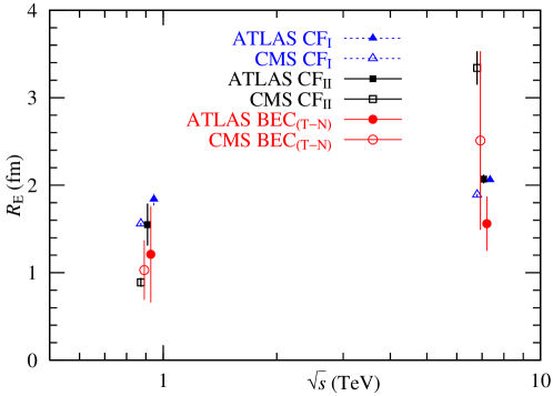
Figure 4: Effective ranges calculated by Eq. (15). The $R$’s estimated by CF_I (E) are shown for comparison.

D1)

We must also elucidate the physical meanings of the three intrinsic parameters $k_{i}$ and weight factor $\alpha_{i}$. From the MC data in [10, 11, 12] and the results of Table 1, we infer the following correspondences:

$$\left\{\begin{array}[]{l}\mbox{1) The first NBD weighted with }\alpha_{1}\leftrightarrow\mbox{ the main part of }\sigma_{\rm ND}.\\ \mbox{2) The second NBD weighted with }\alpha_{2}\leftrightarrow\mbox{ the main part of }\sigma_{\rm SD}\mbox{, and parts of }\sigma_{\rm ND}\mbox{ and }\sigma_{\rm DD}.\\ \mbox{3) The third NBD weighted with }\alpha_{3}\leftrightarrow\mbox{ the main part of }\sigma_{\rm DD}\mbox{, and a part of }\sigma_{\rm SD}.\\ \end{array}\right.$$

Here, $\sigma_{\rm ND}$, $\sigma_{\rm SD}$, and $\sigma_{\rm DD}$ are the cross sections of the ND, SD, and double-diffractive dissociation (DD), respectively.

D2)

In future work, we are planning the following improvements:

The large error bars of $\lambda_{i}^{\rm(T\mathchar 45\relax N)}\ (i=1,\,2)$ must be reduced in future work. For this purpose we must improve the framework of the MD analysis.

D3)

To properly validate the present theoretical formulation [27], we will analyze the MD and BEC ($2.0<\eta<4.5$) obtained by the LHCb collaboration.

Acknowledgments. One of the authors (M.B.) would like to thank his colleagues at the Department of Physics of Shinshu University for their kindness. T. Mizoguchi would like to acknowledge the funding provided by Pres. Y. Hayashi.

Appendix A Monte Carlo data at 7 TeV collected by the ATLAS collaboration and analyzed by Eqs. (1)–(3)

The MC data collected at 0.9 TeV and 7 TeV are presented in [10], which reported the MD results. The total MD is decomposed into three processes: ND, SD, and double-diffractive dissociation (DD), with probability distributions defined by $P_{\rm ND}$, $P_{\rm SD}$, and $P_{\rm DD}$, respectively. The total probability distribution is expressed as $P_{\rm tot}=P_{\rm ND}+P_{\rm SD}+P_{\rm DD}$. The partial and total probability distributions are plotted in Figs. 5 and 6, respectively.

The NBD and D-NBD are calculated by Eqs. (1) and (2), respectively, and the results are shown in Table 11. Obviously, the single-NBD cannot describe the MD. The D-NBD probably constitutes three ensembles with different $\langle n\rangle$ and $k$ values: the first set with ($\langle n\rangle\cong 33$, $k=$2–4), the second set with ($\langle n\rangle=$4–13, $k=$4–16), and the third set with ($\langle n\rangle\cong 10$ and $k=$200–1000). These ensembles appear to reasonably validate the T-NBD framework in the analysis of MD at the LHC. The T-NBD is computed from the total MC data at 7 TeV by Eq. (3). The analysis results are shown in Table 12.

We also analyze the MC data at 0.9 TeV by PYTHIA 6, and at 7 TeV by PHOJET and PYTHIA 8. The results are similar to those in Tables 11 and 12.

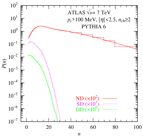
Figure 5: Partial probability distributions $P_{\rm ND}$, $P_{\rm SD}$, and $P_{\rm DD}$ [10] obtained by Eq. (2) (see Table 11).

Table 11: PYTHIA 6 analysis of MD at 7 TeV by the ATLAS collaboration calculated by Eqs. (1) and (2). The magnitude of the error bars is assumed as 10% of the data points. The $\chi^{2}$ values are markedly improved by D-NBD.

PYTHIA 6	ATLAS	single-NBD		D-NBD
7 TeV	ratio	$\langle n\rangle$, $k$	$\chi^{2}$	$i$	$\alpha_{i}$	$\langle n_{i}\rangle$	$k_{i}$	$\chi^{2}$
ND	0.787	$\langle n\rangle=30.17\pm 0.36$	150.4	1	0.814	32.5	2.56	6.84
		$k=2.53\pm 0.04$		2	0.186	13.2	16.85
SD	0.121	$\langle n\rangle=7.08\pm 0.08$	257.3	1	0.716	4.63	7.56	11.75
		$k=15.87\pm 0.80$		2	0.284	10.1	206.7
DD	0.092	$\langle n\rangle=6.15\pm 0.08$	240.7	1	0.798	4.14	4.34	34.00
		$k=10.46\pm 0.50$		2	0.202	9.88	1000.0

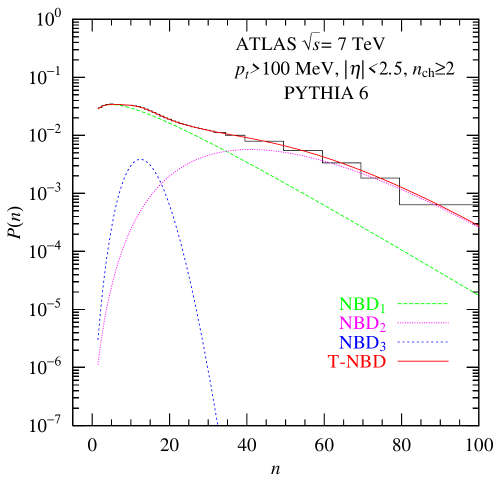
Figure 6: Analysis of the total probability distribution $P_{\rm tot}=P_{\rm ND}+P_{\rm SD}+P_{\rm DD}$ [10] calculated by Eq. (3) (see Table 12).

Table 12: Estimated parameters of T-NBD in the $P_{\rm tot}=P_{\rm ND}+P_{\rm SD}+P_{\rm DD}$ (calculated by Eq. (3)). The magnitude of the error bars is assumed as 10% of the data points.

$i$	$\alpha_{i}$	$\langle n_{i}\rangle$	$k_{i}$	$\chi^{2}$
1	0.711$\pm$0.131	15.37$\pm$3.62	1.56$\pm$0.31
2	0.255$\pm$0.129	47.86$\pm$5.69	7.40$\pm$2.88	0.168
3	0.035$\pm$0.023	12.99$\pm$2.05	1000.0$\pm$551.0

Appendix B An Enlarged KNO scaling function for LHC energies

In this Appendix, we analyze the KNO scaling at LHC energies. Recall that the D-NBD was proposed to explain the KNO scaling violation found at the S$\bar{p}p$S energy ($\sqrt{s}=546$ GeV) [1]. The KNO scaling function in the framework of the T-NBD [20] is given by

$$\psi_{\rm(T\mathchar 45\relax N)}(z=n/\langle n\rangle,\,\alpha_{i},\,k_{i},\,r_{i};\,i=1\sim 3)=\sum_{i=1}^{3}\alpha_{i}\frac{1}{r_{i}}\frac{k_{i}^{k_{i}}(z/r_{i})^{k_{i}-1}}{\Gamma(k_{i})}e^{-k_{i}z/r_{i}}.$$ (17)

After integratin of the KNO scaling variables $z$, the KNO scaling function becomes

$$\int_{0}^{\infty}dz\psi_{\rm(T\mathchar 45\relax N)}(z,\,\alpha_{i},\,k_{i},\,r_{i};\,i=1\sim 3)=\sum_{i=1}^{3}\alpha_{i}=1.0.$$ (18)

The violation of the KNO scaling can be understood studying the energy dependences of the parameters $\alpha_{i}$, $k_{i}$, and $r_{i}$.

The results of Eq. (17) are shown in Fig. 7 and Table 13. The ratio $r_{i}=\langle n_{i}\rangle/\langle n\rangle$ should be large, because the average multiplicities $\langle n_{i}\rangle$ are requaired to be large as $\langle n\rangle$ itself; specifically, $r_{i}\geq 0.33$ ($\langle n_{i}\rangle\geq\langle n\rangle/3$). The KNO scaling functions at 0.9 TeV obtained by the ATLAS and CMS collaborations differed from from those at 7, 8, and 13 TeV (Fig 7). The 0.9 TeV data collected by the CMS collaboration must be constrained by $k_{2}>5$ and $k_{3}>7$ because $z_{3}$ is large (800 or infinity) in the MD analysis. Our KNO scaling analysis also includes the $P(0)$ data at 0.9 and 7 TeV obtained by the CMS collaboration. As shown in Table 13, the violation of KNO scaling occurs through the parameters $\alpha_{i}$ and $r_{i}=\langle n_{i}\rangle/\langle n\rangle$ ($i=1\sim 3$).

Figure 7: Analysis of KNO data collected by the ATLAS and CMS collaborations. The KNO scaling functions were computed by Eq. (17).

Table 13: Analysis (by Eq. (17)) of KNO data at 0.9 and 7.0 TeV collected by the ATLAS and CMS collaboration.

	$i$	$\alpha_{i}$	$r_{i}$	$k_{i}$
ATLAS	1	0.761$\pm$0.134	0.84$\pm$0.10	1.79$\pm$0.08
0.9 TeV	2	0.166$\pm$0.006	1.87$\pm$0.03	5.75$\pm$1.62
$\chi^{2}=25.6$	3	0.074$\pm$0.031	0.67$\pm$0.01	11.0$\pm$3.2
ATLAS	1	0.664$\pm$0.067	0.68$\pm$0.09	1.54$\pm$0.10
7.0 TeV	2	0.275$\pm$0.011	1.91$\pm$0.02	4.37$\pm$0.54
$\chi^{2}=27.4$	3	0.061$\pm$0.011	0.41$\pm$0.01	10.0$\pm$1.8
ATLAS	1	0.692$\pm$0.069	0.73$\pm$0.11	1.50$\pm$0.10
8.0 TeV	2	0.235$\pm$0.003	2.00$\pm$0.01	4.61$\pm$0.61
$\chi^{2}=39.28$	3	0.073$\pm$0.015	0.38$\pm$0.01	7.77$\pm$1.34
ATLAS	1	0.751$\pm$0.037	0.81$\pm$0.06	1.27$\pm$0.04
13 TeV	2	0.168$\pm$0.050	2.18$\pm$0.09	4.88$\pm$0.49
$\chi^{2}=43.26$	3	0.081$\pm$0.007	0.35$\pm$0.01	7.33$\pm$0.66
CMS	1	0.575$\pm$0.079	0.75$\pm$0.09	1.51$\pm$0.17
0.9 TeV	2	0.286$\pm$0.050	1.66$\pm$0.04	5.0 (lower limit)
$\chi^{2}=18.80$	3	0.139$\pm$0.043	0.67$\pm$0.04	7.0 (lower limit)
CMS	1	0.809$\pm$0.019	0.83$\pm$0.02	1.42$\pm$0.05
7.0 TeV	2	0.153$\pm$0.009	2.06$\pm$0.05	5.18$\pm$0.33
$\chi^{2}=7.83$	2	0.038$\pm$0.020	0.45$\pm$0.04	15.2$\pm$10.9

References

- [1] C. Fuglesang, La Thuile Multiparticle Dynamics 1989 (1989) 193-210 (World Scientific, Singapore, 1990).
- [2] Z. Koba, H. B. Nielsen and P. Olesen, Nucl. Phys. B 40 (1972) 317.
- [3] A. Giovannini and R. Ugoccioni, Phys. Rev. D 59 (1999) 094020.
- [4] P. Ghosh, Phys. Rev. D 85 (2012) 054017.
- [5] V. Zaccolo [ALICE Collaboration], Nucl. Phys. A 956 (2016) 529.
- [6] For three-component model, see, A. Giovannini and R. Ugoccioni, Phys. Rev. D 68 (2003) 034009.
- [7] G. Aad et al. [ATLAS Collaboration], New J. Phys. 13 (2011) 053033.
- [8] V. Khachatryan et al. [CMS Collaboration], JHEP 1101 (2011) 079.
- [9] I. Zborovsky, J. Phys. G 40 (2013) 055005.
- [10] [ATLAS Collaboration], “Charged particle multiplicities in pp interactions for track MeV at 0.9 and 7 TeV measured with the ATLAS detector at the LHC,” ATLAS-CONF-2010-046: Therein Fig. 19 is useful for our study.
- [11] J. F. Grosse-Oetringhaus and K. Reygers, J. Phys. G 37 (2010) 083001.
- [12] S. Navin, “Diffraction in Pythia,” LUTP-09-23 [arXiv:1005.3894 [hep-ph]].
- [13] I. Zborovsky, Eur. Phys. J. C 78 (2018) 816.
- [14] G. Wilk and Z. Wlodarczyk, J. Phys. G 44 (2017) 015002.
- [15] M. Rybczynski, G. Wilk and Z. Wlodarczyk, Phys. Rev. D 99 (2019) 094045.
- [16] M. Biyajima, O. Miyamura and T. Nakai, in Proc. Multiparticle Dynamics (Research Inst. for Fundamental Physics, Kyoto Univ., 1978), p. 139.
- [17] M. Biyajima, Prog. Theor. Phys. 69 (1983) 966. Addendum: [Prog. Theor. Phys. 70 (1983) 1468].
- [18] M. Biyajima, A. Bartl, T. Mizoguchi, O. Terazawa and N. Suzuki, Prog. Theor. Phys. 84 (1990) 931; Addendum: [Prog. Theor. Phys. 88 (1992) 157].
- [19] T. Mizoguchi and M. Biyajima, Eur. Phys. J. C 70 (2010) 1061.
- [20] M. Biyajima and T. Mizoguchi, Eur. Phys. J. A 54 (2018) 105.
- [21] T. Mizoguchi and M. Biyajima, JPS Conf. Proc. 26 (2019) 031032.
- [22] G. Aad et al. [ATLAS Collaboration], Eur. Phys. J. C 75 (2015) 466.
- [23] V. Khachatryan et al. [CMS Collaboration], JHEP 1105 (2011) 029.
- [24] R. Aaij et al. [LHCb Collaboration], JHEP 1712 (2017) 025.
- [25] M. Biyajima, Phys. Lett. 137B, 225 (1984) Addendum: [Phys. Lett. 140B, 435 (1984)].
- [26] M. Biyajima and N. Suzuki, Prog. Theor. Phys. 73, 918 (1985) Addendum: [Prog. Theor. Phys. 73, 1303 (1985)].
- [27] T. Mizoguchi and M. Biyajima, in preparation.