bayes4psy – an Open Source R Package for Bayesian Statistics in Psychology

Jure Demšar, Grega Repovš, Erik Štrumbelj bayes4psy - an Open Source R Package for Bayesian Statistics in Psychology bayes4psy Research in psychology generates interesting data sets and unique statistical modelling tasks. However, these tasks, while important, are often very specific, so appropriate statistical models and methods cannot be found in accessible Bayesian tools. As a result, the use of Bayesian methods is limited to those that have the technical and statistical fundamentals that are required for probabilistic programming. Such knowledge is not part of the typical psychology curriculum and is a difficult obstacle for psychology students and researchers to overcome. The goal of the bayes4psy package is to bridge this gap and offer a collection of models and methods to be used for data analysis that arises from psychology experiments and as a teaching tool for Bayesian statistics in psychology. The package contains Bayesian t-test and bootstrapping and models for analyzing reaction times, success rates, and colors. It also provides all the diagnostic, analytic and visualization tools for the modern Bayesian data analysis workflow. R, Bayesian statistics, psychology, reaction time, success rate, Bayesian t-test, color analysis, linear model, bootstrap R, Bayesian statistics, psychology, reaction time, success rate, Bayesian t-test, color analysis, linear model, bootstrap Jure Demšar
Faculty of Computer and Information Science
University of Ljubljana
Večna pot 113
1000 Ljubljana, Slovenia
E-mail:

1 Introduction

Through the development of specialized probabilistic models Bayesian data analysis offers a highly flexible, intuitive and transparent alternative to classical statistics. Bayesian approaches were on the sidelines of data analysis throughout much of the modern era of science. Mostly due to the fact that computations required for Bayesian analysis are usually quite complex. But computations that were only a decade or two ago too complex for specialized computers can nowadays be executed on average desktop computers. In part also due to modern Markov chain Monte Carlo (MCMC) methods that make computations tractable for virtually all parametric models. This, along with specialized probabilistic programming languages for Bayesian modelling – such as Stan (Carpenter2017Stan) and JAGS (Plummer2003Jags) – drastically increased the accessibility and usefulness of Bayesian methodology for data analysis. Indeed, Bayesian data analysis is steadily gaining momentum in the 21^st century (Gelman2014Bayesian; Kruschke2014BayesianDataAnalysis; McElreath2018Rethinking), mainly so in natural and technical sciences. Unfortunately, the use of Bayesian data analysis in social sciences remains scarce, most likely due to the steep statistical and technical learning curve of Bayesian methods.

There are many advantages of Bayesian data analysis, such as its ability to work with missing data and combine prior information with data in a natural and principled way. Furthermore, Bayesian methods offer high flexibility through hierarchical modelling and calculated posterior distribution, while calculated posterior parameter values can be used as easily interpretable alternatives to p-values – Bayesian methods provide very intuitive answers, such as “the parameter $\mu$ has a probability of 0.95 of falling inside the [-2, 2] interval” (Dunson2001Commentary; Gelman2014Bayesian; Kruschke2014BayesianDataAnalysis; McElreath2018Rethinking). One of the social sciences that could benefit the most from Bayesian methodology is psychology. The majority of the data that arises in psychological experiments, such as reaction times, success rates, and colors, can be analyzed in a Bayesian manner by using a small set of probabilistic models. Bayesian methodology could also alleviate the replication crisis that is pestering the field of psychology (OpenScience2015Estimating; Schooler2014Metascience; Stanley2018Meta).

The ability to replicate scientific findings is of paramount importance to scientific progress (Baker2016Crisis; McNutt2014Reproducibility; Munafo2017Manifesto). Unfortunately, more and more replication attempts report that they had failed to reproduce original results and conclusions (Amrhein2019Scientists; OpenScience2015Estimating; Schooler2014Metascience). This so-called replication crisis is harmful not only to the authors but to science itself. A recent attempt to replicate 100 studies from three prominent psychology journals (OpenScience2015Estimating) showed that only approximately a third of studies that claimed statistical significance (p value lower than 0.05) also showed statistical significance in replication. Another recent study (Camerer2018Evaluating) tried to replicate systematically selected studies in the social sciences published in Nature and Science between 2010 and 2015, replication attempts were successful only in 13 cases out of 21.

The main reasons behind the replication crisis seem to be poor quality control in journals, unclear writing and inadequate statistical analysis (Hurlbert2019Coup; Wasserstein2016ASA; Wasserstein2019Moving). One of the main issues lies in the desire to claim statistical significance through p-values. Many manuscripts published today repeat the same mistakes even though prominent statisticians prepared extensive guidelines about what to do and mainly what not to do (Hubbard2015Corrupt; Wasserstein2016ASA; Wasserstein2019Moving; Ziliak2019GVaules). Reluctance to adhere to modern statistical practices has led scientist to believe that a more drastic shift in statistical thinking is needed, and some believe that it might come in the form of Bayesian statistics (Dunson2001Commentary; Gelman2014Bayesian; Kruschke2014BayesianDataAnalysis; McElreath2018Rethinking).

The bayes4psy R package provides a state-of-the art framework for Bayesian analysis of psychological data. It incorporates a set of probabilistic models that can be facilitated for analysis of data that arises during many types of psychological experiments. All models are pre-compiled, meaning that users do not need any specialized software or skills (e.g. knowledge of probabilistic programming languages), the only requirements are the R programming language and very basic programming skills (same skills as needed for classical statistical analysis in R). Besides the probabilistic models, the package also incorporates the diagnostic, analytic and visualization tools required for modern Bayesian data analysis. As such the bayes4psy package represents a bridge into the exciting world of Bayesian statistics for all students and researches in the field of Psychology.

2 Models and methods

For statistical computation, that is, sampling from the posterior distributions, the bayes4psy package utilizes Stan (Carpenter2017Stan). Stan is a state-of-the-art platform for statistical modeling and high-performance statistical computation and offers full Bayesian statistical inference with MCMC sampling. It also offers user friendly interfaces with most programming languages used for statistical analysis, including R. R (R2017Language) is one of the most powerful and widespread programming languages for statistics and visualization. Visualizations in the bayes4psy package are based on the ggplot2 package (Wickham2009ggplot).

2.1 Priors

In Bayesian statistics we use prior probability distributions (priors) to express our beliefs about the parameters before any evidence (data) is taken into account. Priors represent an elegant way of intertwining previous knowledge with new facts about the domain of analysis. Prior distributions are usually based on previously conducted and verified research or on knowledge provided by the domain experts. If such data is not available, we usually resort to our own weakly informative, vague prior knowledge.

In the bayes4psy package users are able to express prior knowledge by putting prior distributions on all of the model’s parameters. Users can express their knowledge by using uniform, normal, gamma, or beta distributions. If users do not specify any prior knowledge about the model’s parameters, then flat/improper priors are put on those parameters. For details see the practical illustrations of using the bayes4psy package in Section 3.

2.2 Bayesian t-test

The t-test is probably the most commonly used hypothesis test. We added the Bayesian version of t-test to the bayes4psy package. The t-test is based on Kruschke’s model (Kruschke2013BayesianSupersedesTTest; Kruschke2014BayesianDataAnalysis). The Bayesian t-test uses a scaled and shifted Student’s t distribution (Figure 1). This distribution has three parameters – degrees of freedom ($\nu$), mean ($\mu$) and variance ($\sigma$)).

There are some minor differences between our implementation and Kruschke’s. Instead of pre-defined vague priors for all parameters, we can define custom priors for the $\nu$, $\mu$ and $\sigma$ parameters. Since Kruschke’s main goal was the comparsion between two groups, his implementation models two data sets simultaneously. Our implementation is more flexible, users can model several data sets individually and then make pairwise comparisons or a simultaneous cross comparison between multiple fits. We illustrate the use of the t-test in Section LABEL:sec:stroop.

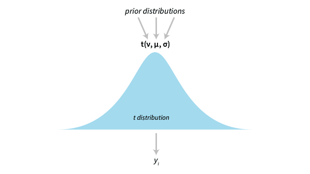
Figure 1: Visualization of the Bayesian t-test. The model has three parameters – degrees of freedom $\nu$, mean $\mu$ and variance $\sigma$. $y_{i}$ denotes $i$-th datum in the provided data set.

2.3 Model for analyzing reaction times

Psychological experiments typically have a hierarchical structure – each subject performs the same test for a number of times, several subjects are then grouped together on their characteristics (e.g. by age, sex, health) and the final statistical analysis is then conducted at the group level. Such structure is ideal for Bayesian hierarchical modelling (Kruschke2014BayesianDataAnalysis).

Our subject-level reaction time model is based on the exponentially modified normal distribution. This distribution has proven to be a suitable interpretation for the long tailed data that arise in reaction time measurements. To model the data at the group level we put hierarchical normal priors on all parameters of the subject-level exponentially modified normal distribution.

The subject level parameters are thus $\mu_{i}$, $\sigma_{i}$ and $\lambda_{i}$, where $i$ is the subject index. And hierarchical normal priors on these parameters are $\mathcal{N}(\mu_{m},\sigma_{m})$ for the $\mu$ parameter, $\mathcal{N}(\mu_{s},\sigma_{s})$ for the $\sigma$ parameter and $\mathcal{N}(\mu_{l},\sigma_{l})$ for the $\lambda$ parameter. Figure 2 is a graphical representation of the Bayesian reaction time model. For a practical application of this model see Section 3.1.

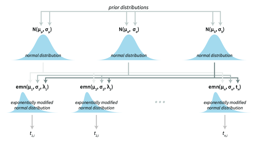
Figure 2: Visualization of the Bayesian reaction time model. The model has a hierarchical structure, reaction times belonging to each individual subject ($t_{n,i}$ depicts $i$-th reaction time of the subject $n$) are used to construct exponentially modified normal distributions at the subject level. Parameters of subject level distributions are then connected at the group level by using normal distributions, which can then be used for group level analysis.

2.4 Model for analyzing success rates

The success rate model is based on the Bernoulli-Beta model that is found in most Bayesian statistics textbooks (Gelman2014Bayesian; Kruschke2014BayesianDataAnalysis; McElreath2018Rethinking). This model is used for modelling binary data, in our case whether or not a subject solves a psychological task.

The success rates model also has a hierarchical structure. The success rate of individual subjects is modelled using Bernoulli distributions, where the $p_{i}$ is the success rate of subject $i$. A reparametrized Beta distribution, $\operatorname{Beta}(p\tau,(1-p)\tau)$, is used as a hierarchical prior on subject-level parameters, where $p$ is the group level success rate and $\tau$ is the scale parameter. A graphical representation of our hierarchical success rate model can be seen in Figure 3. For a practical application of this model see Section 3.1.

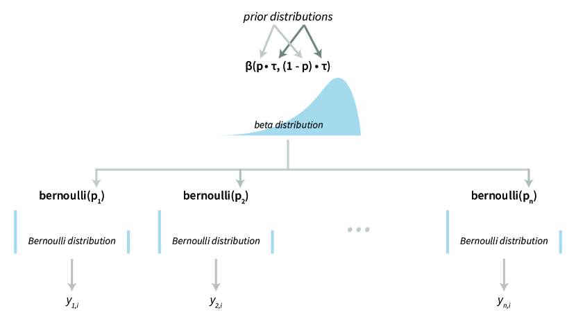
Figure 3: Visualization of the Bayesian success rate model. The model has a hierarchical structure, data about success of individual subjects ($y_{n,i}$ depicts success on the $i$-th attempt of the subject $n$) is used for fitting Bernoulli distributions on the subject level. Parameters of subject level distributions are then connected at the group level with a Beta distribution.

2.5 Model for analysis of sequential tasks

In some psychological experiments the data have a time component or are ordered in some other way. For example, when subjects participate in a sequence of questions or tasks. To model how a subject’s performance changes over time, we implemented a hierarchical linear normal model.

The sequence for each individual subject is modelled using a simple linear model with subject-specific slope and intercept. To model the data at the group level we put hierarchical normal priors on all parameters of the subject-level linear models. The parameters of subject $i$ are thus $\alpha_{i}$ for the intercept and $\beta_{i}$ for the slope of the linear model along with $\sigma_{i}$ for modelling errors of the fit (residuals). And hierarchical normal priors on these parameters are $\mathcal{N}(\mu_{\alpha},\sigma_{\alpha})$ for the intercept ($\alpha$), $\mathcal{N}(\mu_{\beta},\sigma_{\beta})$ for the slope ($\beta$) parameter, along with $\mathcal{N}(\mu_{\sigma},\sigma_{\sigma})$ for the residuals ($\sigma$).

A graphical representation of the model is shown in Figure 4. For a practical application of this model see Section 3.2.

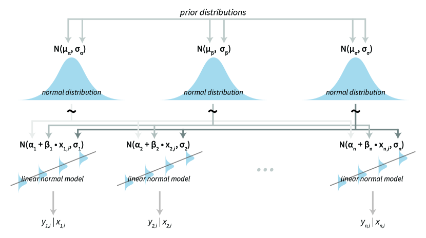
Figure 4: Visualization of the hierarchical linear model. The model has a hierarchical structure, linear normal models are fitted on the subject level from data belonging to each particular subject. Since the ordering of results is important input data come in pairs of dependent (e.g. result or answer) and independent variables (e.g. time or the question index), $y_{n,i}|x_{n,i}$ depicts the value of the $i$-th dependent variable given the value of the independent variable $i$ for the subject $n$. Parameters of subject level distributions are joined on the group level by using normal distributions. These distributions can then be used for group level analysis of the data.

2.6 Model for analysis of color based tasks

Color stimuli and subject responses in psychological experiments are most commonly defined through the RGB color model. The name of the model comes from the initials of the three additive primary colors, red, green and blue. These colors are also the three components of the model, each component has a value from 1 to 255 which defines the presence of a particular color. Since defining and analyzing colors through the RGB model is not very user friendly or intuitive, our Bayesian model is capable of working with both the RGB and HSV color models. HSV (hue, saturation and value) is an alternative representation of the RGB model that is much easier to read and interpret for most human beings.

The Bayesian color model works in a component-wise fashion – six distributions (three for the RGB components and three for the HSV components) are fitted to data for each component individually. For RGB components we use normal distributions (truncated to the [0, 255] interval). In the HSV case, we used normal distributions (truncated to the [0, 1] interval) for saturation and value components and the von Mises distribution for the hue component. The von Mises distribution (also known as the circular normal distribution) is a close approximation to the normal distribution wrapped on the [0, 2pi] interval. A visualization of our Bayesian model for colors can be seen in Figure 5 and its practical application in Section LABEL:sec:afterimages.

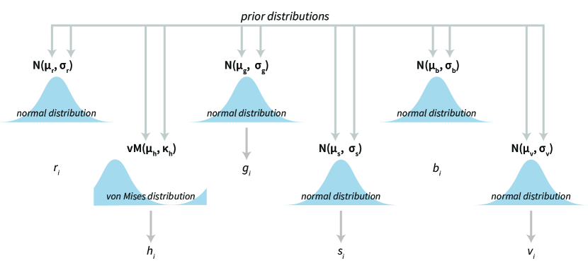
Figure 5: Visualization of the Bayesian color model. The model is composed of six parts. Three parts are used to describe the RGB (red, green, blue) color model components and three parts are used to describe the HSV (hue, saturation, value) color model components. All components, except hue, are modeled with normal distributions, while hue is modelled with the von Mises distribution – a circular normal distribution.

2.7 Bayesian bootstrap

Bootstrapping is a commonly used resampling technique for estimating statistics on a population by sampling a data set with replacement. It is usually used to for evaluating measures of accuracy (such as the mean, bias, standard deviation, confidence intervals …) to sample estimates. It allows estimation of the sampling distribution of almost any statistic using random sampling methods and is as such useful in a wide repertoire of scenarios.

The Bayesian bootstrap inside the bayes4psy package is the analogue of the classical bootstrap (Efron1979Bootstrap). It is based on Rasmus Bååth’s implementation (Baath2016Bootstrap), which in turn is based on methods developed by (Rubin1981Bootstrap). Bayesian bootstrap does not simulate the sampling distribution of a statistic estimating a parameter, but instead simulates the posterior distribution of the parameter. The statistical model underlying the Bayesian bootstrap can be characterized by drawing weights from a uniform Dirichlet distribution with the same dimension as the number of data points, these draws are then used for calculating the statistic in question and weighing the data (Baath2016Bootstrap). For more details about the implementation see (Baath2016Bootstrap) and (Rubin1981Bootstrap).

2.8 Methods for fitting and analyzing Bayesian fits

This section provides a quick overview of all the methods for fitting and analyzing the models described in previous sections. For a more detailed description of each function readers are invited to consult the documentation and examples that are provided along with the R package.

The first set of functions constructs a Bayesian model from input data. Users can also use these functions to define priors (for an example, see the second part of the Section 3.1), set the number of MCMC iterations along with several other parameters of the MCMC algorithm (some basic MCMC settings are described in the documentation of this package, for more advanced settings consult the official Stan (Carpenter2017Stan) documentation).

• b_ttest is a function for fitting the Bayesian t-test model, the input data is a vector of normally distributed real numbers.

• b_linear to construct the hierarchical linear model for analyzing sequential tasks users have to provide three data vectors – $x$ a vector containing values of the in dependant variable (time, question index …), $y$ a vector containing values of the dependant variable (subject’s responses) and $s$ a vector containing ids of subjects used for denoting that $x_{i}$/$y_{i}$ pair belongs to subject $i$.

• b_reaction_time input data to the Bayesian reaction time model consists of two vectors – vector $t$ includes reaction times while vector $s$ is used for linking reaction times with subjects.

• b_success_rate to fit the Bayesian success rate model users have to provide two data vectors. The first vector $r$ contains results of an experiment with binary outcomes (e.g. success/fail, hit/miss …) and the second vector $s$ is used to link results to subjects.

• b_color input data to this model is a three column matrix or a data.frame where each column represents one of the components of the chosen color model (RGB or HSV). If the input data are provided in the HSV format then users also have to set the $hsv$ parameter to TRUE.

• b_bootstrap the mandatory input into the Bayesian bootstrap function is the input data and the statistics function. The input data can be in the form of a vector, matrix or a data.frame.

Before interpreting the results, users can use the following functions to check if the models provide a good representation of the data:

• plot_trace draws the Markov chain trace plot for main parameters of the model, providing a visual way to inspect sampling behavior and assess mixing across chains and convergence.

• plot_fit draws the fitted distribution against the input data. With hierarchical models we can use the subjects parameter to draw fits on the subject level.

• plot_fit_hsv a special function for inspecting the fit of the color model by using a color wheel like visualization of HSV components.

For a summary of the posterior with Monte Carlo standard errors and confidence intervals users can use the summary or print/show functions.

• summary prints summary statistics of the main model’s parameters.

• print, show prints a more detailed summary of the model’s parameters. It includes estimated means, Monte Carlo standard errors (se_mean), confidence intervals, effective sample size (n_eff, a crude measure of effective sample size), and the R-hat statistic for measuring auto-correlation. R-hat measures the potential scale reduction factor on split chains and equals 1 at convergence (Brooks1998General; Gelman1992Inference).

Users can also extract samples from the posterior for further analysis:

• get_parameters returns a data.frame of model’s parameters. In hierarchical models this returns a data.frame of group level parameters.

• get_subject_parameters can be used to extract subject level parameters from hierarchical models.

The compare_means function can be used for comparison of parameters that represent means of the fitted models, to visualize these means one can use the plot_means function and for visualizing the difference between means the plot_means_difference function. All comparison functions (functions that print or visualize difference between fitted models) also offer the option of defining the region of practical equivalence (rope) by setting the rope parameter.

• compare_means prints and returns a data.frame containing the comparison results, can be used for comparing two or multiple models at the same time.

• plot_means_difference visualizes the difference of means between two or multiple models at the same time.

• plot_means plots the distribution of parameters that depict means, can be used on a single or multiple models at the same time.

• plot_means_hsv a special function for the Bayesian color model that plots means of HSV components by using a color wheel like visualization.

The following set of functions works in a similar fashion as the one for comparing means, the difference is that this one compares entire distributions and not just the means. The comparison is based on drawing a large amount of samples from the distributions.

• compare_distributions prints and returns a data.frame containing the comparison results, can be used for comparing two or multiple models at the same time.

• plot_distributions_difference visualizes the difference of distributions underlying two or multiple fits at the same time.

• plot_distribution plots the distributions underlying the fitted models, can be used on a single or multiple models at the same time.

• plot_distributions_hsv a special function for the Bayesian color model that plots the distribution behind HSV components by using a color wheel like visualization.

3 Illustrations

Below are illustrative practical examples of models in the bayes4psy package. Additional examples can be found in the online repository (https://github.com/bstatcomp/bayes4psy_tools).

For the sake of brevity, we omitted similar visualizations and outputs, e.g. we provided the diagnostic outputs and visualizations only the first time they appered and omitted them later due to similarity.

3.1 The flanker task

In the Eriksen flanker task (Eriksen1974Flanker) participants are presented with an image of an odd number of arrows (usually five or seven). Their task is to indicate the orientation (left or right) of the middle arrow as quickly as possible whilst ignoring the flanking arrows on left and right. There are two types of stimuli in the task: in the congruent condition (e.g. ‘<<<<<<<‘) both the middle arrow and the flanking arrows point in the same direction, whereas in the incongruent condition (e.g. ‘<<<><<<‘) the middle arrow points to the opposite direction of the flanking arrows.

As the participants have to consciously ignore and inhibit the misleading information provided by the flanking arrows in the incongruent condition, the performance in the incongruent condition is robustly worse than in the congruent condition, both in terms of longer reaction times as well as higher proportion of errors. The difference between reaction times and error rates in congruent and incongruent cases is a measure of subject’s ability to focus his or her attention and inhibit distracting stimuli.

In the illustration below we compare reaction times and error rates when solving the flanker task between the control group (healthy subjects) and the test group (subjects suffering from a certain medical condition).

First, we load package bayes4psy and package dplyr for data wrangling. Second, we load the data and split them into control and test groups. For reaction time analysis we use only data where the response to the stimuli was correct:

R> library(bayes4psy) R> library(dplyr)

R> data <- read.table("./data/flanker.csv", sep=""͡, header=TRUE)

R> control_rt <- data group == "control")

R> test_rt <- data group == "test")

The model requires subjects to be indexed from $1$ to $n$. Control group subject indexes range from 22 to 45, so we cast it to 1 to 23.

R> control_rt$subject<-control_{r}t$subject - 21

Now we are ready to fit the Bayesian reaction time model for both groups. The model function requires two parameters – a vector of reaction times $t$ and the vector of subject indexes $s$.

R> rt_control_fit <- b_reaction_time(t=control_rt$rt,s=control_{r}t$subject)

R> rt_test_fit <- b_reaction_time(t=test_rt$rt,s=test_{r}t$subject)

Before we interpret the results, we check MCMC diagnostics and model fit.

plot_trace(rt_control_fit) plot_trace(rt_test_fit)

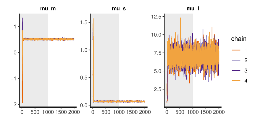
Figure 6: The trace plot for rt_control_fit. The traceplot gives us no cause for concern regarding MCMC convergence and mixing. The trace plot for rt_test_fit is similar. Note that the first 1000 iterations (shaded gray) are used for warmup (tuning of the MCMC algorithm) and are discarded. The next 1000 iterations are used for sampling.

R> print(rt_control_fit)

Inference for Stan model: reaction_time. 4 chains, each with iter=2000; warmup=1000; thin=1; post-warmup draws per chain=1000, total post-warmup draws=4000.

mean se_mean sd 2.5mu[1] 0.46 0.00 0.01 0.44 0.47 4789 1 mu[2] 0.36 0.00 0.01 0.35 0.38 4661 1 … sigma[1] 0.04 0.00 0.01 0.03 0.05 5406 1 sigma[2] 0.03 0.00 0.01 0.02 0.04 5165 1 … lambda[1] 14.41 0.02 1.62 11.59 17.87 4441 1 lambda[2] 11.59 0.02 1.15 9.53 14.01 5271 1 … mu_m 0.51 0.00 0.01 0.48 0.54 5589 1 mu_l 6.86 0.01 0.91 5.12 8.75 5299 1 mu_s 0.07 0.00 0.01 0.06 0.08 4115 1 sigma_m 0.06 0.00 0.01 0.05 0.09 6078 1 sigma_l 4.24 0.01 0.78 3.02 5.99 3940 1 sigma_s 0.02 0.00 0.00 0.01 0.03 3862 1 rt 0.66 0.00 0.02 0.61 0.71 5112 1 rt_subjects[1] 0.53 0.00 0.01 0.51 0.54 4261 1 rt_subjects[2] 0.45 0.00 0.01 0.44 0.47 5654 1 …

R> print(rt_test_fit)

The output above is truncated and shows only values for 2 of the 24 subjects on the subject level of the hierarchical model. The output provides further MCMC diagnostics, which again do not give us cause for concern. The convergence diagnostic Rhat is practically 1 for all parameters and there is little auto-correlation (possibly even some positive auto-correlation) – effective sample sizes (n_eff) are of the order of samples taken and Monte Carlo standard errors (se_mean) are relatively small.

What is a good-enough effective sample sizes depends on our goal. If we are interested in posterior quantities such as the more extreme percentiles, the effective sample sizes should be 10,000 or higher, if possible. If we are only interested in estimating the mean, 100 effective samples is in most cases enough for a practically negligible Monte Carlo error.

We can increase the effective sample size by increasing the amount of MCMC iterations with the iter parameter. In our case we can achieve an effective sample size of 10,000 by setting iter to 4000. Because the MCMC diagnostics give us no reason for concern, we can leave the warmup parameter at its default value of 1000.

R> rt_control_fit <- b_reaction_time(t=control_rt$rt,s=control_{r}t$subject, iter=4000)

R> rt_test_fit <- b_reaction_time(t=test_rt$rt,s=test_{r}t$subject, iter=4000)

Because we did not explicitly define any priors, flat (improper) priors were put on all of the model’s parameters. In some cases, flat priors are a statement that we have no prior knowledge about the experiment results (in some sense). In general, even flat priors can express a preference for a certain region of parameter space. In practice, we will almost always have some prior information and we should incorporate it into the modelling process.

Next, we check whether the model fits the data well by using the plot_fit function. If we set the subjects parameter to FALSE, we will get a less detailed group level fit.

R> plot_fit(rt_control_fit) R> plot_fit(rt_test_fit)

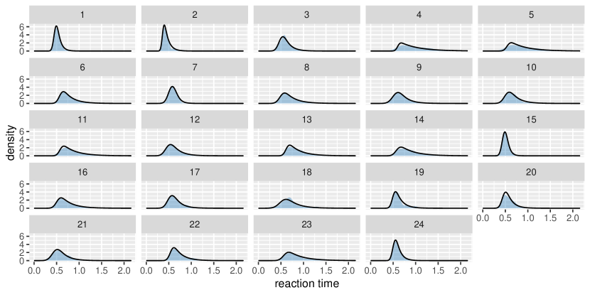
Figure 7: The fit plot for the rt_control_fit. The data are visualized as a blue region while the fit is visualized with a black line. In this case the model fits the underlying data well, similar conclusions can be reached for the test group (rt_test_fit).

We now use the compare_means function to compare reaction times between healthy (control) and unhealthy (test) subjects. In the example below we use a rope (region of practical equivalence) interval of 0.01 s, meaning that differences smaller that 1/100 of a second are deemed as equal. The compare_means function provides a user friendly output of the comparison and also returns the results in the form of a data.frame.

R> rt_control_test <- compare_means(rt_control_fit, fit2=rt_test_fit, rope=0.01)

———- Group 1 vs Group 2 ———- Probabilities: - Group 1 < Group 2: 0.98 +/- 0.00409 - Group 1 > Group 2: 0.01 +/- 0.00304 - Equal: 0.01 +/- 0.00239 95- Group 1 - Group 2: [-0.17, -0.01]

The compare_means function output contains probabilities that one group has shorter reaction times than the other, the probability that both groups are equal (if rope interval is provided) and the 95% HDI (highest density interval, Kruschke2014BayesianDataAnalysis) for the difference between groups. Based on the output we are quite certain (98% +/- 0.5%) that the healthy group’s (rt_control_fit) expected reaction times are lower than the unhealthy group’s (rt_test_fit).

We can also visualize this difference by using the plot_means_difference function. The plot_means function is an alternative for comparing rt_control_fit and rt_test_fit – the function visualizes the parameters that determine the means of each model.

R> plot_means_difference(rt_control_fit, fit2=rt_test_fit, rope=0.01)

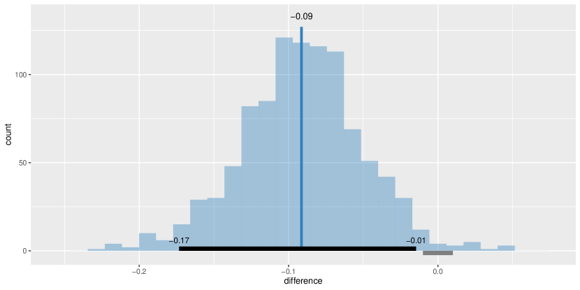
Figure 8: A visualization of the difference between rt_control_fit and rt_test_fit. The histogram visualizes the distribution of the difference, vertical blue line denotes the mean, the black band at the bottom marks the 95% HDI interval and the gray band marks the rope interval. Since the whole 95% HDI of difference is negative and lies outside of the rope interval we can conclude that the statement that healthy subjects are faster than unhealthy ones is most likely correct.

R> plot_means(rt_control_fit, fit2=rt_test_fit)

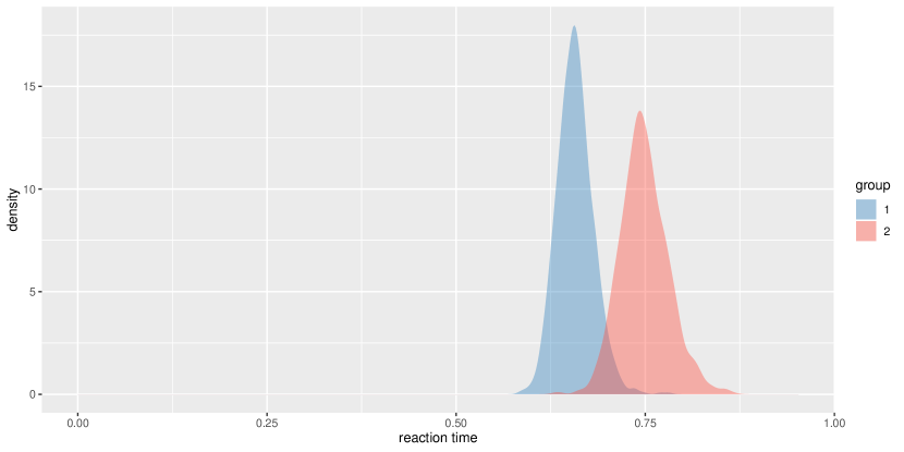
Figure 9: A visualization of means for rt_control_fit and rt_test_fit. Group 1 visualizes means for the healthy subjects and group 2 for the unhealthy subjects.

We can with high probability (98% +/- 0.5%) claim that healthy subjects have faster reaction times when solving the flanker task than unhealthy subjects. Next, we analyze if the same applies to success rates.

The information about success of subject’s is stored as "correct"/"incorrect". However, the Bayesian success rate model requires binary inputs (0/1) so we have to transform the data. Also, like in the reaction time example, we have to correct the indexes of control group subjects.

R> data$result_{n}umeric<-0R>data[data$result == "correct", ]$result_{n}umeric<-1\par R>control_{s}r<-dataR>test_{s}r<-data\par R>control_{s}r$subject <- control_sr$subject-21\par Sincetheonlypriorinformationaboutthesuccessrateofparticipantswasthefactthatsuccessrateislocatedbetween0and1,weusedabetadistributiontoputauniformprioronthe[0,1]interval(weputa$Beta(1, 1)$prioronthe$p$parameter).Weexecutethemodelfittingbyrunningthe\code{b\_success\_rate}functionwithappropriateinputdata.\par\CodeChunk\CodeInput R>p_{p}rior<-b_{p}rior(family="beta",pars=c(1,1))\par R>priors<-list(c("p",p_{p}rior))\par R>sr_{c}ontrol_{f}it<-b_{s}uccess_{r}ate(r=control_{s}r$result_{n}umeric,s=control_{s}r$subject,priors=priors,iter=4000)\par R>sr_{t}est_{f}it<-b_{s}uccess_{r}ate(r=test_{s}r$result_{n}umeric,s=test_{s}r$subject,priors=priors,iter=4000)\par TheprocessforinspectingBayesianfitsisthesameandtheresultsaresimilarasabove,soweomitthem.Whenvisuallyinspectingthequalityofthefit(the\code{plot\_fit}function)wecansetthe\code{subjects}parameterto\code{FALSE},whichvisualizesthefitonthegrouplevel.Thisoffersaquicker,butlessdetailedmethodofinspection.\par\CodeChunk\CodeInput R>plot_{t}race(sr_{c}ontrol_{f}it)R>plot_{t}race(sr_{t}est_{f}it)\par R>print(sr_{c}ontrol_{f}it)R>print(sr_{t}est_{f}it)\par R>plot_{f}it(sr_{c}ontrol_{f}it,subjects=FALSE)R>plot_{f}it(sr_{t}est_{f}it,subjects=FALSE)\par Sincediagnosticfunctionsshownopressingissuesandthefitslookgoodwecanproceedwiththeactualcomparisonbetweenthetwofittedmodels.Wewillagainestimatethedifferencebetweentwogroupswith\code{compare\_means}.\par\CodeChunk\CodeInput R>sr_{c}ontrol_{t}est<-compare_{m}eans(sr_{c}ontrol_{f}it,fit2=sr_{t}est_{f}it)\par----------Group1vsGroup2----------Probabilities:-Group1<Group2:0.53+/-0.01052-Group1>Group2:0.47+/-0.0105295-Group1-Group2:[-0.02,0.02]\par Aswecanseethesuccessratebetweenthetwogroupsisnotthatdifferent.Sincetheprobabilitythathealthygroupismoresuccessfulisonly53\%(+/-1\%)andthe95\%HDIofthedifference([0.02,0.02])includesthe0wecannotclaiminequality\cite[citep]{(\@@bibref{AuthorsPhrase1Year}{Kruschke2014BayesianDataAnalysis}{\@@citephrase{, }}{})}.Wecanvisualizethisresultbyusingthe\code{plot\_means\_difference}function.\par\LTX@newpage\par\CodeChunk\CodeInput R>plot_{m}eans_{d}ifference(sr_{c}ontrol_{f}it,fit2=sr_{t}est_{f}it)\par\begin{figure}[ht]\centering\includegraphics[width=433.62pt]{flanker_plot_means_difference_sr.pdf}\@@toccaption{{\lx@tag[ ]{{10}}{{\bf Avisualizationofthedifferencebetweenthe\code{sr\_control\_fit}andthe\code{sr\_test\_fit}.}Histogramvisualizesthedistributionofthedifference,verticalbluelinedenotesthemeandifferenceandtheblackbandatthebottommarksthe95\%HDIinterval.Sincethe95\%HDIofdifferenceincludesthevalueof0wecannotclaiminequality.Ifweusedaropeintervalandthewholeropeintervalliedinthe95\%HDIintervalwecouldclaimequality.}}}\@@caption{{\lx@tag[: ]{{Figure 10}}{{\bf Avisualizationofthedifferencebetweenthe\code{sr\_control\_fit}andthe\code{sr\_test\_fit}.}Histogramvisualizesthedistributionofthedifference,verticalbluelinedenotesthemeandifferenceandtheblackbandatthebottommarksthe95\%HDIinterval.Sincethe95\%HDIofdifferenceincludesthevalueof0wecannotclaiminequality.Ifweusedaropeintervalandthewholeropeintervalliedinthe95\%HDIintervalwecouldclaimequality.}}}\@add@centering\end{figure}\par\LTX@newpage\par$

3.2 Adaptation level

In the adaptation level experiment participants had to assess weights of the objects placed in their hands by using a verbal scale: very very light, very light, light, medium light, medium, medium heavy, heavy, very heavy and very very heavy. The task was to assess the weight of an object that was placed on the palm of their hand. To standardize the procedure the participants had to place the elbow on the desk, extend the palm and assess the weight of the object after it was placed on their palm by slight up and down movements of their arm. During the experiment participants were blinded by using non-transparent fabric. In total there were 15 objects of the same shape and size but different mass (photo film canisters filled with metallic balls). Objects were grouped into three sets:

• light set: 45 g, 55 g, 65 g, 75 g, 85 g (weights 1 to 5),

• medium set: 95 g, 105 g, 115 g, 125 g, 135 g (weights 6 to 10),

• heavy set: 145 g, 155 g, 165 g, 175 g, 185 g (weights 11 to 15).

The experimenter sequentially placed weights in the palm of the participant and recorded the trial index, the weight of the object and participant’s response. The participants were divided into two groups, in group 1 the participants first assessed the weights of the light set in ten rounds within which all five weights were weighted in a random order. After completing the 10 rounds with the light set, the experimenter switched to the medium set, without any announcement or break. The participant then weighted the medium set across another 10 rounds of weighting the five weights in a random order within each round. In group 2 the overall procedure was the same, the only difference being that they started with the 10 rounds of the heavy set and then performed another 10 rounds of weighting of the medium set. Importantly, the weights within each set were given in random order and the experimenter switched between sets seamlessly without any break or other indication to the participant.

We will use the bayes4psy package to show that the two groups provide different assessment of the weights in the second part of the experiment even though both groups are responding to weights from the same (medium) set. The difference is very pronounced at first but then fades away with subsequent assessments of medium weights. This is congruent with the hypothesis that each group formed a different adaptation level during the initial phase of the task, the formed adaptation level then determined the perceptual experience of the same set of weights at the beginning of the second part of the task.

We will conduct the analysis by using the hierarchical linear model and the Bayesian t-test. First we have to construct fits for the second part of the experiment for each group independently. The code below loads and prepares the data, just like in the previous example, subject indexes have to be mapped to a [1, n] interval. We will use to ggplot2 package to fine-tune graph axes and properly annotate graphs returned by the bayes4psy package.

R> library(bayes4psy) R> library(dplyr) R> library(ggplot2)

R> data <- read.table("./data/adaptation_level.csv", sep=""͡, header=TRUE)

R> group1 <- data R> group2 <- data

R> n1 <- length(unique(group1$subject))R>n2<-length(unique(group2$subject))

R> group1$subject<-plyr::mapvalues(group1$subject, from=unique(group1$subject),to=1:n1)R>group2$subject <- plyr::mapvalues(group1$subject,from=unique(group1$subject), to=1:n2)

R> group1_part2 <- group1 R> group2_part2 <- group2

Once the data is prepared we can fit the Bayesian models, the input data comes in the form of three vectors, $x$ stores indexes of the measurements, $y$ subject’s responses and $s$ indexes of subjects. The warmup and iter parameters are set in order to achieve an effective sample size of 10,000.

R> fit1 <- b_linear(x=group1