Mean Dimension of Ridge Functions

Abstract

We consider the mean dimension of some ridge functions of spherical Gaussian random vectors of dimension $d$. If the ridge function is Lipschitz continuous, then the mean dimension remains bounded as $d\to\infty$. If instead, the ridge function is discontinuous, then the mean dimension depends on a measure of the ridge function’s sparsity, and absent sparsity the mean dimension can grow proportionally to $\sqrt{d}$. Preintegrating a ridge function yields a new, potentially much smoother ridge function. We include an example where, if one of the ridge coefficients is bounded away from zero as $d\to\infty$, then preintegration can reduce the mean dimension from $O(\sqrt{d})$ to $O(1)$.

65C05, 65D30, 65D32

1 Introduction

Numerical integration of high dimensional functions is a very common and challenging problem. Under the right conditions, quasi-Monte Carlo (QMC) sampling and randomized QMC (RQMC) sampling can be very effective. A good result can be expected from (R)QMC if the following conditions, described in more detail below, all hold:

1. the (R)QMC points have highly uniform low dimensional projections,

2. the integrand is nearly a sum of low dimensional parts, and

3. those parts are regular enough to benefit from (R)QMC.

The first condition is a usual property of (R)QMC points. In a series of papers, Griebel, Kuo and Sloan [9, 10, 11] address the third condition by showing that the low dimensional parts of $f$ (defined there via the ANOVA decomposition) are at least as smooth as the original integrand and are often much smoother. They include conditions under which lower order ANOVA terms of functions with discontinuities (jumps) or discontinuities in their first derivative (kinks) are smooth. An alternative form of regularity, instead of smoothness, is for the low dimensional parts to have QMC-friendly discontinuities as described in [35]. In this article we explore sufficient conditions for the remaining second condition to hold. We use the mean dimension [26] to quantify the extent to which low dimensional components dominate the integrand.

This article is focused on ridge functions defined over $\mathbb{R}^{d}$. Ridge functions take the form $f(\boldsymbol{x})=g(\Theta^{\mathsf{T}}\boldsymbol{x})$ for an orthonormal projection matrix $\Theta\in\mathbb{R}^{d\times r}$ where $r\ll d$, with $r=1$ being an important special case. Ridge functions are useful here because we can find their integrals via low dimensional integration or even closed form expressions. That lets us investigate the impact of some qualitative features of $f$ on the integration problem. Additionally, many functions in science and engineering are well approximated by ridge functions with small values of $r$ [3], so good performance on ridge functions could extend well to many functions in the natural sciences. As one more example, the value of a European option under geometric Brownian motion is a ridge function of the Brownian increments and this is what allows the formula of Black and Scholes to be applied [8].

Our main finding is that there is an enormous difference between functions $g(\cdot)$ with jumps and functions with kinks. This is perhaps surprising. Based on criteria for finite variation in the sense of Hardy and Krause, one might have thought that a jump in $d$ dimensions would be similar to a kink in $d-1$. Instead, we find that for Lipschitz continuous $g:\mathbb{R}\to\mathbb{R}$, the mean dimension of $f$ is bounded as $d\to\infty$ and that bound can be quite low. For $g$ with step discontinuities, we find that the mean dimension can easily grow proportionally to $\sqrt{d}$. These effects were seen empirically in [28] where ridge functions were used to illustrate a scrambled Halton algorithm. Preintegration [12] turns a ridge function over $[0,1]^{d}$ with a jump into one with a kink, and ridge functions of Gaussian variables containing a jump can even become infinitely differentiable. The resulting Lipschitz constant need not be small. For a linear step function we find that preintegration can either increase mean dimension or reduce it from $O(\sqrt{d})$ to $O(1)$.

An outline of this paper is as follows. Section 2 provides notation and background concepts related to quasi-Monte Carlo and mean dimension. Section 3 introduces ridge functions and establishes upper bounds on their mean dimension in terms of Hölder and Lipschitz conditions and some spatially varying relaxations of those conditions. Corollary 3.3 there shows that a ridge function with Lipschitz constant $C$ and variance $\sigma^{2}$ cannot have a mean dimension larger than $rC^{2}/\sigma^{2}$ in any dimension $d\geqslant r\geqslant 1$ for any projection $\Theta\in\mathbb{R}^{d\times r}$. Section 4 considers ridge functions with jumps. They can have mean dimension growing proportionally to $\sqrt{d}$ and sparsity of $\theta$ makes a big difference. Section 5 considers the effects of preintegration on ridge functions. The preintegrated functions are also ridge functions with a Hölder constant no worse than the original function had. Preintegration can either raise or lower mean dimension. We give an example step function where preintegration leaves the mean dimension asymptotically proportional to $\sqrt{d}$ with an increased lead constant. In another example, preintegration can change the mean dimension from growing proportionally to $\sqrt{d}$ to having a finite bound as $d\to\infty$. Section 6 computes some mean dimensions using Sobol’ indices. Section 7 has conclusions, and a discussion of how generally these results may apply. Section 8 is an appendix containing the longer proofs.

2 Background and notation

We use $\varphi(\cdot)$ for the standard Gaussian probability density function and $\Phi(\cdot)$ for the corresponding cumulative distribution function. We consider integration with respect to a $d$-dimensional spherical Gaussian measure,

$$\mu\equiv\int_{\mathbb{R}^{d}}f(\boldsymbol{x})(2\pi)^{-d/2}e^{-\|\boldsymbol{x}\|^{2}/2}\,\mathrm{d}\boldsymbol{x}=\int_{(0,1)^{d}}f(\Phi^{-1}(\boldsymbol{x}))\,\mathrm{d}\boldsymbol{x},$$

where the quantile function $\Phi^{-1}(\cdot)$ is applied componentwise. The (R)QMC approximations to $\mu$ take the form $\hat{\mu}=(1/n)\sum_{i=1}^{n}\tilde{f}(\boldsymbol{x}_{i})$ for points $\boldsymbol{x}_{i}\in(0,1)^{d}$ and $\tilde{f}(\cdot)=f\circ\Phi^{-1}(\cdot)$. The distribution of $\boldsymbol{x}$ is denoted $\mathcal{N}(0,I_{d})$ or simply $\mathcal{N}(0,I)$ if $d$ is understood from context.

QMC and Koksma-Hlawka

For QMC, the Koksma-Hlawka inequality [14]

(1) $$|\hat{\mu}-\mu|\leqslant D^{*}_{n}\times\|\tilde{f}\|_{\mathrm{HK}}$$

bounds the error in terms of the star discrepancy $D^{*}_{n}=D^{*}_{n}(\boldsymbol{x}_{1},\dots,\boldsymbol{x}_{n})$ of the points used and the total variation of $f$ in the sense of Hardy and Krause. Constructions with $D_{n}^{*}=O(\log(n)^{d-1}/n)$ are known [21, 5, 31], proving that QMC can be asymptotically better than Monte Carlo (MC) sampling which has a root mean squared error of $O(n^{-1/2})$. That argument requires $\|\tilde{f}\|_{\mathrm{HK}}<\infty$ which requires at a minimum that $f$ be a bounded function on $\mathbb{R}^{d}$. Scrambled net RQMC has a root mean squared error that is $o(n^{-1/2})$ for any $f\in L^{2}$ without requiring bounded variation [24].

Kinks and jumps

A kink function is continuous with a discontinuity in its first derivative along some manifold. Griebel et al. [12] consider kink functions of the form $\max(\phi(\boldsymbol{x}),0)$ where $\phi$ is smooth. The kink takes place within the set $\{\boldsymbol{x}\mid\phi(\boldsymbol{x})=0\}$. A jump function has a step discontinuity along some manifold. Griewank et al. [12] consider jump functions of the form $\theta(\boldsymbol{x})\times\max(\phi(\boldsymbol{x}),0)$ where $\theta$ is also smooth. There can be jump discontinuities within the set $\{\boldsymbol{x}\mid\phi(\boldsymbol{x})=0\}$. When $\theta(\cdot)=\phi(\cdot)$, the result is a kink function. In the rest of this paper, $\theta$ denotes a unit vector.

ANOVA and mean dimension

The ANOVA decomposition applies to any measurable and square integrable function of $d$ independent random inputs. In our case, those inputs will be either $\mathbb{U}(0,1)$ or $\mathcal{N}(0,1)$.

We use $1{:}d$ for $\{1,2,\dots,d\}$, and for $u\subseteq 1{:}d$, we write $|u|$ for the cardinality of $u$ and $-u$ for the complement $1{:}d\setminus u$. The point $\boldsymbol{x}\in\mathbb{R}^{d}$ has components $x_{j}$ for $j\in 1{:}d$. The point $\boldsymbol{x}_{u}\in\mathbb{R}^{|u|}$ has the components $x_{j}$ for $j\in u$. We abbreviate $\boldsymbol{x}_{-\{j\}}$ to $\boldsymbol{x}_{-j}$. For $u\subseteq 1{:}d$ and points $\boldsymbol{x},\boldsymbol{z}\in\mathbb{R}^{d}$, the hybrid point $\boldsymbol{y}=\boldsymbol{x}_{u}{:}\boldsymbol{z}_{-u}$ has $y_{j}=x_{j}$ for $j\in u$ and $y_{j}=z_{j}$ otherwise.

The ANOVA decomposition [15, 33, 6] of $f:[0,1]^{d}\to\mathbb{R}$ is $f(\boldsymbol{x})=\sum_{u\subseteq 1{:}d}f_{u}(\boldsymbol{x})$ where $f_{u}$ depends on $\boldsymbol{x}$ only through $\boldsymbol{x}_{u}$. For these functions, the line integral $\mathbb{E}(f_{u}(\boldsymbol{x})\mid\boldsymbol{x}_{-j})=0$ whenever $j\in u$ and from that it follows that $\mathbb{E}(f_{u}(\boldsymbol{x})f_{v}(\boldsymbol{x}))=0$ when $u\neq v$ and then

$$\sigma^{2}=\sigma^{2}(f)=\mathbb{E}((f(\boldsymbol{x})-\mu)^{2})=\sum_{u:|u|>0}\sigma^{2}_{u}$$

for variance components $\sigma^{2}_{u}=\sigma^{2}_{u}(f)=\mathbb{E}(f_{u}(\boldsymbol{x})^{2})$ for $u\neq 0$ and $\sigma^{2}_{\varnothing}=0$.

The mean dimension of $f$ (in the superposition sense) is

$$\nu(f)=\frac{\sum_{u\subseteq 1{:}d}|u|\sigma^{2}_{u}}{\sum_{u\subseteq 1{:}d}\sigma^{2}_{u}}.$$

If we choose $u\subseteq 1{:}d$ with probability proportional to $\sigma^{2}_{u}$ then $\nu(f)$ is the average of $|u|$. Effective dimension is commonly defined via a high quantile of that distribution such as the 99’th percentile [2]. Such an effective dimension could well be larger than the mean dimension but it is more difficult to ascertain.

The mean dimension and a few other quantities that we use are not well defined when $\sigma^{2}=0$. In such cases, $f$ is constant almost everywhere and we will not ordinarily be interested in integrating it. We assume below, without necessarily stating it every time, that $\sigma^{2}>0$.

Sobol’ indices are used to quantify the importance of a variable or more generally a subset of them. We will use the (unnormalized) Sobol’ total index for variable $j$,

$$\overline{\tau}^{2}_{j}=\sum_{u:j\in u}\sigma_{u}^{2}.$$

More generally, for $u\subset 1{:}d$, we set $\overline{\tau}^{2}_{u}=\sum_{v:v\cap u\neq\varnothing}\sigma^{2}_{v}$. An easy identity from [19] gives $\nu(f)=(1/\sigma^{2})\sum_{j=1}^{d}\overline{\tau}^{2}_{j}$. Sobol’ [34] shows that

$$\overline{\tau}_{j}^{2}=\frac{1}{2}\mathbb{E}\bigl{(}\bigl{(}f(\boldsymbol{x}_{-j}{:}x_{j})-f(\boldsymbol{x}_{-j}{:}z_{j})\bigr{)}^{2}\,\bigr{)}$$

when $\boldsymbol{x}$ and $\boldsymbol{z}$ are independent random vectors with the same product distribution on $\mathbb{R}^{d}$. As a result we find that

(2) $$\nu(f)=\frac{1}{2\sigma^{2}}\mathbb{E}\Biggl{(}\,\sum_{j=1}^{d}\bigl{(}f(\boldsymbol{x})-f(\boldsymbol{x}_{-j}{:}z_{j})\bigr{)}^{2}\Biggr{)}.$$

The expectation in the numerator of $\nu(f)$ is a $2d$-dimensional integral over independent $\boldsymbol{x}$ and $\boldsymbol{z}$. It is commonly evaluated by (R)QMC.

Low effective dimension

Applying (1) componentwise yields

$$|\hat{\mu}-\mu|\leqslant\sum_{u}D_{n}^{*}(\boldsymbol{x}_{1,u},\dots,\boldsymbol{x}_{n,u})\times\|\tilde{f}_{u}\|_{\mathrm{HK}}.$$

The coordinate discrepancies $D_{n}^{*}(\boldsymbol{x}_{1,u},\dots,\boldsymbol{x}_{n,u})$ are known to decay rapidly when $|u|$ is small [5]. If also $\|\tilde{f}_{u}\|_{\mathrm{HK}}$ is negligible when $|u|$ is not small then $\tilde{f}$ can be considered to have low effective dimension and an apparent $O(n^{-1})$ error for QMC can be observed. Some other ways to decompose a function into a sum of $2^{d}$ functions, one for each subset of $1{:}d$, are described in [17]. For a survey of effective dimension methods in information based complexity, see [36].

To avoid the dependence on finite variation and to control the logarithmic terms we will use a version of RQMC known as scrambled nets. Under scrambled net sampling [23] each $\boldsymbol{x}_{i}\sim\mathbb{U}(0,1)^{d}$, while collectively $\boldsymbol{x}_{1},\dots,\boldsymbol{x}_{n}$ remain digital nets with probability one, retaining their low discrepancy. The mean squared error of scrambled net sampling decomposes as

(3) $$\mathbb{E}((\hat{\mu}-\mu)^{2})=\sum_{|u|>0}\mathbb{E}\Bigl{(}\Bigl{(}\frac{1}{n}\sum_{i=1}^{n}\tilde{f}_{u}(\boldsymbol{x}_{i})\Bigr{)}^{2}\Bigr{)}=\sum_{|u|>0}\mathrm{Var}\Bigl{(}\frac{1}{n}\sum_{i=1}^{n}\tilde{f}_{u}(\boldsymbol{x}_{i})\Bigr{)}$$

where expectation refers to randomness in the $\boldsymbol{x}_{i}$ [24]. If $\tilde{f}\in L^{2}$, then

(4) $$\mathrm{Var}\Bigl{(}\frac{1}{n}\sum_{i=1}^{n}\tilde{f}_{u}(\boldsymbol{x}_{i})\Bigr{)}=o\Bigl{(}\frac{1}{n}\Bigr{)}\quad\text{and}\quad\mathrm{Var}\Bigl{(}\frac{1}{n}\sum_{i=1}^{n}\tilde{f}_{u}(\boldsymbol{x}_{i})\Bigr{)}\leqslant\Gamma\frac{\sigma^{2}_{u}}{n},$$

for some gain coefficient $\Gamma<\infty$ [25]. If also $\partial^{u}\tilde{f}_{u}\in L^{2}$ then

(5) $$\mathrm{Var}\Bigl{(}\frac{1}{n}\sum_{i=1}^{n}\tilde{f}_{u}(\boldsymbol{x}_{i})\Bigr{)}=O\Bigl{(}\frac{\log(n)^{|u|-1}}{n^{3}}\Bigr{)}.$$

If large $|u|$ have negligible $\sigma^{2}_{u}$ and small $|u|$ are smooth enough for (5) to hold then RQMC may attain nearly $O(n^{-3/2})$ root mean squared error. The logarithmic factors in (5) cannot make the variance much larger than the MC rate because the bound in (4) applies for finite $n$.

The ANOVA decomposition of $f$ on $\boldsymbol{x}\in\mathbb{R}^{d}$ is essentially the same as that of $\tilde{f}$ on $(0,1)^{d}$. Specifically, $f_{u}(\boldsymbol{x})=\tilde{f}_{u}(\Phi^{-1}(\boldsymbol{x}))$.

Discontinuities can lead to severe deterioration in the asymptotic behavior of RQMC. He and Wang [13] obtain MSE rates of $O(n^{-1-1/(2d-1)}(\log n)^{2d/(2d-1)})$ for jump discontinuities of the form $f(\boldsymbol{x})=g(\boldsymbol{x})1\{\boldsymbol{x}\in\Omega\}$ where the set $\Omega$ has a boundary with $(d-1)$-dimensional Minkowski content. When $\Omega$ is the Cartesian product of a hyper-rectangle and a $d^{\prime}$-dimensional set with a boundary of $(d^{\prime}-1)$-dimensional Minkowski content, then $d^{\prime}$ takes the place of $d$ in their rate. The smaller $d^{\prime}$ is, the more ‘QMC-friendly’ the discontinuity is.

3 Ridge functions

We let $\boldsymbol{x}\sim\mathcal{N}(0,I)$, choose an orthonormal matrix $\Theta\in\mathbb{R}^{d\times r}$, and define the ridge function

(6) $$f(\boldsymbol{x})=g\bigl{(}\Theta^{\mathsf{T}}\boldsymbol{x}\bigr{)},$$

where $g:\mathbb{R}^{r}\to\mathbb{R}$. We must always have $d\geqslant r$ because otherwise $\Theta^{\mathsf{T}}\Theta=I_{r}$ is impossible to attain. Our main interest is in $r\ll d$. Ridge functions can also be defined for $\boldsymbol{x}\sim\mathbb{U}[0,1]^{d}$ but then the domain of $g$ becomes a complicated polyhedron called a zonotope [3].

When $r=1$, we write

(7) $$f(\boldsymbol{x})=g\bigl{(}\theta^{\mathsf{T}}\boldsymbol{x}\bigr{)},$$

where $g:\mathbb{R}\to\mathbb{R}$. Then, because $\theta^{\mathsf{T}}\boldsymbol{x}\sim\mathcal{N}(0,1)$ we find that

$$\mu=\int_{-\infty}^{\infty}g(z)\varphi(z)\,\mathrm{d}z\quad\text{and}\quad\sigma^{2}=\int_{-\infty}^{\infty}(g(z)-\mu)^{2}\varphi(z)\,\mathrm{d}z.$$

We can get the answer $\mu$ and the corresponding RMSE $\sigma/\sqrt{n}$ under MC by one dimensional integration. For some $g$, one or both of these quantities are available in closed form. Note that $\mu$ and $\sigma^{2}$ above are both independent of $\theta$ and even of $d$. For more general $r\geqslant 1$ we find that $\mu$ and $\sigma^{2}$ are $r$-dimensional integrals that do not depend on $\Theta$ or on $d\geqslant r$. Apart from a few remarks, we focus mostly on the case with $r=1$.

By symmetry we can take all $\theta_{j}\geqslant 0$. It is reasonable to expect that sparse vectors $\theta$ will make the problem of intrinsically lower dimension. Sparsity is typically defined via small values of $\sum_{j=1}1_{\theta_{j}\neq 0}$. It is common to use instead a proxy measure $\|\theta\|_{1}$, with smaller values representing greater sparsity, relaxing an $L_{0}$ quantity to an $L_{1}$ quantity. By this measure, the ‘least sparse’ unit vectors are of the form $\theta_{j}=\pm 1/\sqrt{d}$ while sparsest are of the form $\pm e_{j}$ where $e_{j}$ is the $j$’th standard Euclidean basis vector.

We will need some fractional absolute moments of the $\mathcal{N}(0,1)$ distribution. For $\eta>-1$ define

(8) $$M_{\eta}=\int_{-\infty}^{\infty}|y|^{\eta}\varphi(y)\,\mathrm{d}y=\frac{2^{\eta/2}}{\sqrt{\pi}}\Gamma\Bigl{(}\frac{\eta+1}{2}\Bigr{)}.$$

This is from formula (18) in an unpublished report of Winkelbauer [37]. It can be verified directly by change of variable to $x=y^{2}/2$.

Theorem 3.1.

Let $f$ be a ridge function described by (6) for $1\leqslant r\leqslant d$, where $g:\mathbb{R}^{r}\to\mathbb{R}$ satisfies a Hölder condition $|g(\boldsymbol{y})-g(\boldsymbol{y}^{\prime})|\leqslant C\|\boldsymbol{y}-\boldsymbol{y}^{\prime}\|^{\alpha}$ for $C<\infty$, $0<\alpha\leqslant 1$, and $\boldsymbol{y},\boldsymbol{y}^{\prime}\in\mathbb{R}^{r}$. Then the mean dimension of $f$ satisfies

(9) $$\nu(f)\leqslant\Bigl{(}\frac{C}{\sigma}\Bigr{)}^{2}2^{\alpha-1}M_{2\alpha}\times\sum_{j=1}^{d}\biggl{(}\,\sum_{k=1}^{r}\Theta_{jk}^{2}\biggr{)}^{\alpha},$$

where $\sigma^{2}=\mathrm{Var}(f(\boldsymbol{x}))$ does not depend on $d$.

Proof 3.2.

Let $\boldsymbol{x}$ and $\boldsymbol{z}$ be independent $\mathcal{N}(0,I_{d})$ random vectors. For $j\in 1{:}d$, let $\Theta_{j\cdot}$ be the $j$’th row of $\Theta$ as a row vector. Then $\Theta^{\mathsf{T}}\boldsymbol{x}_{-j}{:}z_{j}-\Theta^{\mathsf{T}}\boldsymbol{x}=\Theta_{j\cdot}^{\mathsf{T}}(z_{j}-x_{j})$. Next

(10) $$\overline{\tau}^{2}_{j} =\frac{1}{2}\mathbb{E}\Bigl{(}\bigl{(}g(\boldsymbol{x})-g(\boldsymbol{x}_{-j}{:}z_{j})\bigr{)}^{2}\Bigr{)}\leqslant\frac{C^{2}}{2}\mathbb{E}\Bigl{(}\|\Theta_{j\cdot}^{\mathsf{T}}(z_{j}-x_{j})\|^{2\alpha}\Bigr{)}=2^{\alpha-1}C^{2}\|\Theta_{j\cdot}^{\mathsf{T}}\|^{2\alpha}M_{2\alpha}$$

because $(z_{j}-x_{j})/\sqrt{2}\sim\mathcal{N}(0,1)$. Summing over $j$ gives (10). Finally, $\sigma^{2}$ depends on the distribution of $g(\boldsymbol{y})$ for $\boldsymbol{y}\sim\mathcal{N}(0,I_{r})$ which is independent of $d$.

If $\alpha\geqslant 1/2$, then we recognize $\sum_{j=1}^{d}\bigl{(}\sum_{k=1}^{r}\Theta_{jk}^{2}\bigr{)}^{\alpha}$ as $\|\Theta^{\mathsf{T}}\|_{2,2\alpha}^{2\alpha}$ where $\|\cdot\|_{p,q}$ is a matrix $L_{p,q}$ norm [22]. For $\alpha<1/2$, we get $q<1$ and this is then not a norm. If $Q\in\mathbb{R}^{d\times d}$ is an orthogonal matrix, then $g(\Theta^{\mathsf{T}}\boldsymbol{x})=g((Q\Theta)^{\mathsf{T}}(Q\boldsymbol{x}))$. Now $Q\boldsymbol{x}\sim\mathcal{N}(0,I)$ so we can replace $\|\Theta^{\mathsf{T}}\|^{2\alpha}_{2,2\alpha}$ in (9) by $\inf_{Q}\|\Theta^{\mathsf{T}}Q^{\mathsf{T}}\|^{2\alpha}_{2,2\alpha}$. For $\alpha=1$, we get $\|\Theta^{\mathsf{T}}\|^{2\alpha}_{2,2\alpha}=\sum_{j=1}^{d}\sum_{k=1}^{r}\Theta_{jk}^{2}=\|\Theta\|_{F}^{2}$, the squared Frobenius norm of $\Theta$, and the bound in (9) simplifies to reveal a proportional dependence on $r$.

Corollary 3.3.

Let $f$ be a ridge function described by (6) where $g$ is Lipschitz continuous with constant $C$ and $\Theta\in\mathbb{R}^{d\times r}$ with $\Theta^{\mathsf{T}}\Theta=I_{r}$, for $r\leqslant d<\infty$. Then

$$\nu(f)\leqslant r\times\Bigl{(}\frac{C}{\sigma}\Bigr{)}^{2}$$

where $\sigma^{2}=\mathrm{Var}(f(\boldsymbol{x}))$ does not depend on $d$.

Proof 3.4.

Take $\alpha=1$ in Theorem 3.1.

The bound in Theorem 3.1 and its corollaries is conservative. It allows for the possibility that $|g(\boldsymbol{y})-g(\boldsymbol{y}^{\prime})|=C\|\boldsymbol{y}-\boldsymbol{y}^{\prime}\|^{\alpha}$ for all pairs of points $\boldsymbol{y},\boldsymbol{y}^{\prime}\in\mathbb{R}^{r}$. If that would hold for $r=1$ and $\alpha=1$, then it would imply that $g$ is linear. To see why, note that any triangle with points $(y_{1},g(y_{1}))$, $(y_{2},g(y_{2}))$, and $(y_{3},g(y_{3}))$, for distinct $y_{j}$ would have one angle equal to $\pi$. A linear function would then have mean dimension $1$, the smallest possible value when $\sigma^{2}>0$. A less conservative bound is in Section 3.1 below. The next result show that the bound has a dimensional effect when $\alpha<1$.

Corollary 3.5.

Let $f$ be a ridge function given by (7) with $r=1$, where $g$ is Hölder continuous with constant $C$ and exponent $\alpha\in(0,1)$ and $\theta\in\mathbb{R}^{d}$ is a unit vector for $1\leqslant d<\infty$. Then

$$\nu(f)\leqslant\Bigl{(}\frac{C}{\sigma}\Bigr{)}^{2}2^{\alpha-1}M_{2\alpha}d^{1-\alpha}.$$

Proof 3.6.

From Theorem 3.1, $\nu(f)\leqslant 2^{\alpha-1}M_{2\alpha}(C/\sigma)^{2}\sum_{j=1}^{d}|\theta_{j}|^{2\alpha}$. The largest value this can take arises for $\theta_{j}=\pm 1/\sqrt{d}$. Then $\sum_{j=1}^{d}|\theta_{j}|^{2\alpha}=d\times d^{-2\alpha/2}=d^{1-\alpha}$ and so $\nu(f)\leqslant 2^{\alpha-1}M_{2\alpha}C^{2}\sigma^{-2}d^{1-\alpha}$ as required.

3.1 Spatially varying Hölder and Lipschitz constants

A Lipschitz or Hölder inequality provides a bound on $|g(\boldsymbol{y})-f(\boldsymbol{y}^{\prime})|$ that holds for all $\boldsymbol{y},\boldsymbol{y}^{\prime}\in\mathbb{R}^{r}$. The numerator in $\nu(f)$ is a weighted average of $|f(\boldsymbol{x})-f(\boldsymbol{x}_{-j}{:}z_{j})|^{2}$ over points $\boldsymbol{x},\boldsymbol{z}$ and indices $j$, and for a ridge function that reduces to a weighted average of $|g(\boldsymbol{y})-g(\boldsymbol{y}^{\prime})|^{2}$ Applying a Lipschitz or Hölder inequality bounds an $L_{2}$ quantity by the square of an $L_{\infty}$ quantity.

We say that $g$ satisfies a spatially varying Hölder condition if for some $0<\alpha\leqslant 1$ there is a function $C(\boldsymbol{y})$ such that

(11) $$|g(\boldsymbol{y})-g(\boldsymbol{y}^{\prime})|\leqslant C(\boldsymbol{y})\|\boldsymbol{y}-\boldsymbol{y}^{\prime}\|^{\alpha}$$

holds for all $\boldsymbol{y}$ and $\boldsymbol{y}^{\prime}$. If $\alpha=1$, then $g$ satisfies a spatially varying Lipschitz condition. The well known locally Lipschitz condition is different. It requires that every $\boldsymbol{y}$ be within a neighborhood $U_{\boldsymbol{y}}$ on which $g$ has a finite Lipschitz constant $C(\boldsymbol{y})$. Equation (11) is stronger because it also bounds $|g(\boldsymbol{y})-g(\boldsymbol{y}^{\prime})|$ for $\boldsymbol{y}^{\prime}\not\in U_{\boldsymbol{y}}$.

We will use a Hölder inequality via $1<p\leqslant\infty$ and $q$ satisfying $1/p+1/q=1$ to slightly modify the proof in Theorem 3.1. Under (11)

$$\sigma^{2}\nu(f) \leqslant\frac{1}{2}\sum_{j=1}^{d}\mathbb{E}\bigl{(}C(\Theta^{\mathsf{T}}\boldsymbol{x})^{2}\|\Theta_{j\cdot}^{\mathsf{T}}(z_{j}-x_{j})\|^{2\alpha}\bigr{)}$$

$$\leqslant\frac{1}{2}\mathbb{E}(|C(\boldsymbol{y})|^{2p})^{1/p}\sum_{j=1}^{d}\mathbb{E}\bigl{(}\|\Theta_{j\cdot}^{\mathsf{T}}(z_{j}-x_{j})\|^{2\alpha q}\bigr{)}^{1/q}\quad\text{(with $\boldsymbol{y}\sim\mathcal{N}(0,I_{r})$)}$$

(12) $$\leqslant 2^{\alpha-1}\mathbb{E}(|C(\boldsymbol{y})|^{2p})^{1/p}M_{2\alpha q}^{1/q}\sum_{j=1}^{d}\|\Theta_{j\cdot}^{\mathsf{T}}\|^{2\alpha}.$$

Allowing $p=1$ would have made $q=\infty$ and then the supremum norm of $|x_{j}-z_{j}|$ would be infinite, leading to a useless bound. For $p=\infty$, we interpret $\mathbb{E}(|C(\boldsymbol{y})|^{2p})^{1/p}$ as $\sup_{\boldsymbol{y}}|C(\boldsymbol{y})|^{2}$ recovering Theorem 3.1. The bound (12) simplifies for $r=1$ and for $\alpha=1$. Under both simplifications,

$$\nu(f)\leqslant\frac{1}{\sigma^{2}}\mathbb{E}(C(\boldsymbol{y})^{2p})^{1/p}M_{2q}^{1/q}.$$

To get a finite bound for $\nu(f)$ it suffices for $C(\boldsymbol{y})$ to have a finite moment of order $2+\epsilon$ for some $\epsilon>0$.

3.2 A kink function

As a prototypical kink function, consider $f$ given by (7) with $g(y)=(y-t)_{+}$ for some threshold $t$. This $g$ is Lipschitz continuous with $C=1$. Using indefinite integrals $\int x\varphi(x)\,\mathrm{d}x=-\varphi(x)+c$ and $\int x^{2}\varphi(x)\,\mathrm{d}x=\Phi(x)-x\varphi(x)+c$, the first two moments of $f(\boldsymbol{x})$ are

$$\mu(t) =\int_{-\infty}^{\infty}\max(y-t,0)\varphi(y)\,\mathrm{d}y=\varphi(t)-t\Phi(-t),\quad\text{and}$$

$$(\mu^{2}+\sigma^{2})(t) =\int_{-\infty}^{\infty}\max(y-t,0)^{2}\varphi(y)\,\mathrm{d}y=\Phi(-t)(1+t^{2})-t\varphi(t),\quad\text{so}$$

$$\sigma^{2}(t) =\Phi(-t)(1+t^{2})-t\varphi(t)-\varphi(t)^{2}+2t\varphi(t)\Phi(-t)-t^{2}\Phi(-t)^{2}.$$

Because $C=M_{2}=1$, we get $\nu(f)\leqslant 1/\sigma^{2}(t)$. For $t=0$, we get $\mu=\varphi(0)$ and $\sigma^{2}=\mathbb{E}(g(y)^{2})-\mu^{2}=1/2-1/(2\pi)$ and then

$$\nu(f)\leqslant\frac{1}{1/2-1/(2\pi)}=\frac{2\pi}{\pi-1}\doteq 2.933,$$

for any $d\geqslant 1$ and any unit vector $\theta\in\mathbb{R}^{d}$.

3.3 The least sparse case

The least sparse unit vectors have all $\theta_{j}=\pm 1/\sqrt{d}$. Because $\mathcal{N}(0,I)$ is symmetric we may take $\theta_{j}=1/\sqrt{d}$. In this case, it is easy to compute $\nu(f)$ using Sobol’ indices. By symmetry, $\nu(f)$ equals a three dimensional integral

(13) $$\frac{d}{2\sigma^{2}}\int_{\mathbb{R}^{3}}\biggl{(}g\Bigl{(}\frac{\sqrt{d-1}x+y}{\sqrt{d}}\Bigr{)}-g\Bigl{(}\frac{\sqrt{d-1}x+z}{\sqrt{d}}\Bigr{)}\biggr{)}^{2}\varphi(x)\varphi(y)\varphi(z)\,\mathrm{d}x\,\mathrm{d}y\,\mathrm{d}z,$$

for any $d\geqslant 1$. Furthermore, by comparing results for $d^{\prime}\ll d$ to those for $d$ we can see some impact from sparsity because the least sparse unit vector for dimension $d^{\prime}$ will give the same answer as a very sparse $d$ dimensional vector with $d-d^{\prime}$ zeros and the remaining components equal.

4 Jumps

While both kinks and jumps may have smooth low dimensional ANOVA components, jumps do not necessarily have the same low mean dimension. They are also sensitive to sparsity of $\theta$.

4.1 Linear step functions

First we consider a step function $1\{\theta^{\mathsf{T}}\boldsymbol{x}>t\}$. We get upper and lower bounds for the mean dimension of this function in terms of the nominal dimension $d$ and $\|\theta\|_{1}$, our sparsity measure. Over the range from sparsest to least sparse $1\leqslant\|\theta\|_{1}\leqslant\sqrt{d}$.

Theorem 4.1.

Let $f(\boldsymbol{x})=1\{\theta^{\mathsf{T}}\boldsymbol{x}>t\}$ for a threshold $t\geqslant 0$ and a unit vector $\theta\in\mathbb{R}^{d}$. Then, for $d\geqslant 2$,

$$\nu(f)\leqslant\frac{\|\theta\|_{1}}{\Phi(t)\Phi(-t)\sqrt{2\pi}}\Bigl{(}\sqrt{2}+2\sqrt{\log(\|\theta\|_{1}^{-1}d)}\Bigr{)}=O\bigl{(}\sqrt{d\log(d)}\bigr{)}.$$

Proof 4.2.

See Section 8.1 of the Appendix.

The $O(\sqrt{d\log(d)})$ rate in Theorem 4.1 arises for $\|\theta\|_{1}=\sqrt{d}$. More generally we get

$$O(\|\theta\|_{1}\sqrt{\log(d/\|\theta\|_{1})})=O\bigl{(}\|\theta\|_{1}\sqrt{\log(d)}\bigr{)}.$$

For instance, if $\theta$ has $r\geqslant 1$ components equal to $\pm 1/\sqrt{r}$ and the rest equal to zero, then the upper bound is $O(r^{1/2}\sqrt{\log(d/r)})$. There can thus be a significant improvement due to sparsity of $\theta$.

Theorem 4.3.

Let $f(\boldsymbol{x})=1\{\theta^{\mathsf{T}}\boldsymbol{x}>t\}$ for a threshold $t\geqslant 0$ and a unit vector $\theta\in\mathbb{R}^{d}$. Then, for $d\geqslant 2$,

$$\nu(f)\geqslant\frac{\|\theta\|_{1}}{\Phi(t)\Phi(-t)2^{3/2}\pi}e^{-t^{2}-1}.$$

Proof 4.4.

See Section 8.3 of the Appendix.

The proof of Theorem 4.3 requires a certain lower bound on a bivariate Gaussian probability. We did not find many such lower bounds in the literature, so this may be new and may be of independent interest.

Lemma 4.5.

Let

$$\begin{pmatrix}x\\ y\end{pmatrix}\sim\mathcal{N}\left(\begin{pmatrix}0\\ 0\end{pmatrix},\begin{pmatrix}1&\rho\\ \rho&1\end{pmatrix}\right)$$

with $\rho\geqslant 0$ and choose $t\geqslant 0$. Then

$$\Pr(x>t,y<t)\geqslant\frac{1}{2\pi}\Bigl{(}\frac{1-\rho}{1+\rho}\Bigr{)}^{1/2}\exp\Bigl{(}-\frac{t^{2}}{1+\rho}-1\Bigr{)}.$$

Proof 4.6.

See Section 8.2 of the Appendix.

Choosing $\theta=(\pm 1,\pm 1,\dots,\pm 1)/\sqrt{d}$ in Theorem 4.3 provides an example of a set of jump functions with mean dimension bounded below by a positive multiple of $\sqrt{d}$. Here again sparsity plays a role in the bound.

The bounds in both Theorems 4.1 and 4.3 depend on $t$. The upper bound argument in Theorem 4.1 uses a mean value approximation where $\varphi(0)$ could be replaced by a value just over $\varphi(-t)$, yielding for $t>0$ that

$$\nu(f)\leqslant\frac{2\sqrt{\log(d/\|\theta\|_{1})}}{\Phi(t)\Phi(-t)}\Bigl{(}o(1)+\varphi(t)(1+o(1))\Bigr{)}=O\biggl{(}\frac{2\sqrt{\log(d/\|\theta\|_{1})}}{\Phi(t)}\frac{t^{2}+1}{t}\biggr{)}$$

by a Mills’ ratio inequality as $d\to\infty$. As a result the upper bound is not as sensitive to large $t$ as the presence of $\Phi(-t)$ in the denominator from Theorem 4.1 would suggest.

The case $t=0$ is simpler. We find

$$\nu(f) =\frac{1}{\Phi(0)^{2}}\sum_{j=1}^{d}\Pr\bigl{(}\theta^{\mathsf{T}}\boldsymbol{x}>0,\,\theta^{\mathsf{T}}\boldsymbol{x}+\theta_{j}(z_{j}-x_{j})<0\bigr{)}$$

$$=4\sum_{j=1}^{d}\int_{0}^{\infty}\varphi(x)\Phi\Bigl{(}-\rho_{j}x/\sqrt{\smash[b]{1-\rho_{j}^{2}}}\,\Bigr{)}\,\mathrm{d}\boldsymbol{x},\quad\rho_{j}=1-\theta_{j}^{2}$$

$$=\sum_{j=1}^{d}\frac{2}{\pi}\Bigl{(}\frac{\pi}{2}-\arctan\Bigl{(}-\rho_{j}/{\sqrt{\smash[b]{1-\rho_{j}^{2}}}}\,\Bigr{)}\Bigr{)},$$

using a definite integral from Section 2.5.2 of [30]. After some algebra

(14) $$\nu(f)=\frac{2}{\pi}\sum_{j=1}^{d}\arcsin(|\theta_{j}|)\geqslant\frac{2}{\pi}\|\theta\|_{1}.$$

Now $\arcsin(x)=x+O(x^{3})$ as $|x|\to 0$. Therefore $\nu(f)\to 2\|\theta\|_{1}/\pi$ holds if $\|\theta\|_{\infty}\to 0$ holds as $d\to\infty$. Thus there is no asymptotic $\sqrt{\log(d)}$ factor when $t=0$ and, from the details of our proof, we suspect it is not present for other $t$.

4.2 More general indicator functions

It is reasonable to expect indicator functions to have such large mean dimension for more general sets than just half spaces in $\mathbb{R}^{d}$ under a spherical Gaussian distribution. Here we sketch a generalization. First, for an indicator function $f(\boldsymbol{x})=1\{\boldsymbol{x}\in\Omega\}$ of a measurable set $\Omega\subset\mathbb{R}^{d}$ we have

(15) $$\nu(f)=\sum_{j=1}^{d}\mathbb{E}\bigl{(}\Pr(\boldsymbol{x}\in\Omega\mid\boldsymbol{x}_{-j})\Pr(\boldsymbol{x}\in\Omega^{c}\mid\boldsymbol{x}_{-j})\bigr{)}\bigm{/}\bigl{[}\mu(1-\mu)\bigr{]}$$

for $\mu=\Pr(\boldsymbol{x}\in\Omega)$. The numerator expectations are with respect to random $\boldsymbol{x}_{-j}$, and (15) holds for any distribution on $\boldsymbol{x}$ with independent components, including $\mathbb{U}(0,1)^{d}$ and $\mathcal{N}(0,I)$. We work with the latter case in what follows.

As in [10, 11] we take $\Omega=\{\boldsymbol{x}\mid\phi(\boldsymbol{x})\geqslant 0\}$ and place conditions on $\phi$. Let $\phi\in C^{\infty}(\mathbb{R}^{d})$ be strictly monotone in each coordinate $x_{j}$. Without loss of generality, suppose that $\phi$ is strictly increasing in each $x_{j}\sim\mathcal{N}(0,1)$. Suppose additionally that $\lim_{z_{j}\to\infty}\phi(\boldsymbol{x}_{-j}{:}z_{j})>0$ and $\lim_{z_{j}\to-\infty}\phi(\boldsymbol{x}_{-j}{:}z_{j})<0$ for all $j$ and all $\boldsymbol{x}_{-j}\in\mathbb{R}^{d-1}$.

For any $\boldsymbol{x}_{-j}$, there is a unique value $z_{j}\in\mathbb{R}$ for which $\phi(\boldsymbol{x}_{-j}{:}z_{j})=0$. We write $\boldsymbol{z}^{*}=\boldsymbol{x}_{-j}{:}z_{j}$ and sometimes suppress its dependence on $\boldsymbol{x}_{-j}$. We can make a linear approximation to the boundary of $\Omega$ at $\boldsymbol{z}^{*}$ via $\boldsymbol{x}^{\mathsf{T}}\theta^{*}=t^{*}$ where both $\theta^{*}$, the normalized gradient of $\phi$, and $t^{*}$ depend on $\boldsymbol{z}^{*}$. By monotonicity of $\phi$, each $\theta^{*}_{j}>0$. Let

$$\delta_{j}(\boldsymbol{x}_{-j}) \equiv\Pr(\phi(\boldsymbol{x})\geqslant 0\mid\boldsymbol{x}_{-j})\Pr(\phi(\boldsymbol{x})<0\mid\boldsymbol{x}_{-j})$$

$$=\Phi\Biggl{(}\frac{\sum_{\ell\neq j}x_{\ell}\theta^{*}_{\ell}(\boldsymbol{x}_{-j})-t^{*}(\boldsymbol{x}_{-j})}{\theta^{*}_{j}(\boldsymbol{x}_{-j})}\Biggr{)}\Phi\Biggl{(}\frac{t^{*}(\boldsymbol{x}_{-j})-\sum_{\ell\neq j}x_{\ell}\theta^{*}_{\ell}(\boldsymbol{x}_{-j})}{\theta^{*}_{j}(\boldsymbol{x}_{-j})}\Biggr{)},\quad\text{and}$$

$$\delta(\boldsymbol{x}) =\sum_{j=1}^{d}\delta_{j}(\boldsymbol{x}_{-j}).$$

Now $\nu(f)=\mathbb{E}(\delta(\boldsymbol{x}))/[\mu(1-\mu)]$. In words, $\mathbb{E}(\delta(\boldsymbol{x}))$ is what we would get by sampling $\boldsymbol{x}\sim\mathcal{N}(0,I)$, finding the $d$ boundary points $\boldsymbol{z}^{*}$ corresponding to the $d$ component directions $x_{j}$, summing the corresponding $\delta_{j}$ values, and averaging the results over all samples. Each point $\boldsymbol{x}$ leads to consideration of $d$ points $\boldsymbol{z}^{*}\in\partial\Omega$. This process produces an unequally weighted average over points $\boldsymbol{z}^{*}\in\partial\Omega=\{\boldsymbol{z}\mid\phi(\boldsymbol{z})=0\}$ of a sum of $\delta_{j}$ values determined by the tangent plane at $\boldsymbol{z}^{*}$.

For a linear $\phi$, we get $\partial\Omega=\{\boldsymbol{z}\mid\theta^{\mathsf{T}}\boldsymbol{z}=t\}$, and we find from Theorem 4.3 that $\mathbb{E}(\delta(\boldsymbol{x}))$ is then bounded below by a multiple of $\|\theta\|_{1}$ which can be as large as $\sqrt{d}$. For more general $\phi$, the boundary set $\partial\Omega$ is no longer an affine flat, the sparsity measure $\|\theta^{*}\|_{1}$ varies spatially over $\partial\Omega$, and so does the length $t^{*}$. A large mean dimension, comparable to $\sqrt{d}$, could arise if $\phi$ has a nonsparse gradient over an appreciable proportion of $\partial\Omega$.

If the assumption that $\lim_{z_{j}\to\infty}\phi(\boldsymbol{x}_{-j}{:}z_{j})>0$ fails, or if $\lim_{z_{j}\to-\infty}\phi(\boldsymbol{x}_{-j}{:}z_{j})<0$ fails, for some value $\boldsymbol{x}_{-j}$, then we can no longer find the corresponding point $z_{j}$. In that case, the given value of $j$ and $\boldsymbol{x}_{-j}$ contribute nothing to the numerator of $\nu(f)$. The mean dimension can still be large due to contributions from other values of $\boldsymbol{x}_{-j}$ and from other $j$. A similar issue came up in [11] where existence of $z_{j}$ for every $\boldsymbol{x}_{-j}$ proved not to be satisfied by an integrand from computational finance, and also proved not to be necessary for the smoothing effect of ANOVA to hold.

4.3 Cusps of general order

For $d\geqslant 1$ and $\boldsymbol{x}\in[0,1]^{d}$, consider a cusp of order $p>0$ given by

(16) $$f_{d,p}(\boldsymbol{x})=\biggl{(}\,\sum_{j=1}^{d}x_{j}-(d-1)\biggr{)}_{+}^{p}$$

taking $f_{d,0}(\boldsymbol{x})=1\{\sum_{j=1}^{d}x_{j}>d-1\}$. Now $\|f_{d,0}\|_{\mathrm{HK}}=\infty$ for $d\geqslant 2$ [27], $\|f_{d,1}\|_{\mathrm{HK}}=\infty$ for $d\geqslant 3$, and more generally $\|f_{d,p}\|_{\mathrm{HK}}=\infty$ for $d\geqslant p+2$. The higher the dimension, the greater smoothness is required to have finite variation. The boundary $\{\boldsymbol{x}\mid\sum_{j}x_{j}=d-1\}$ is not parallel to any of the coordinate axes, so this integrand is not QMC-friendly in any way.

These functions are carefully constructed to be among the simplest with the prescribed level of smoothness. As a result, we may find their mean dimension analytically.

Theorem 4.7.

The function $f_{d,p}$ defined above for $\boldsymbol{x}\sim\mathbb{U}[0,1]^{d}$ has mean dimension

$$\nu(f_{d,p}) =d\times\frac{\frac{\Gamma(2p+1)}{\Gamma(2p+d+1)}-\bigl{(}\frac{\Gamma(p+1)}{\Gamma(p+2)}\bigr{)}^{2}\frac{\Gamma(2p+3)}{\Gamma(2p+d+2)}}{\frac{\Gamma(2p+1)}{\Gamma(2p+d+1)}-\bigl{(}\frac{\Gamma(p+1)}{\Gamma(p+d+1)}\bigr{)}^{2}}.$$

Proof 4.8.

See Section 8.4 of the Appendix.

The functions $f_{d,0}$ have jumps. Taking $p=0$ in Theorem 4.7 yields

$$\nu(f_{d,0}) =\frac{d\bigl{(}\frac{\Gamma(1)}{\Gamma(d+1)}-\bigl{(}\frac{\Gamma(1)}{\Gamma(2)}\bigr{)}^{2}\frac{\Gamma(3)}{\Gamma(d+2)}\bigr{)}}{\frac{\Gamma(1)}{\Gamma(d+1)}-\bigl{(}\frac{\Gamma(1)}{\Gamma(d+1)}\bigr{)}^{2}}=d\times\frac{1-\frac{2}{d+1}}{1-\frac{1}{d!}}.$$

Thus $\nu(f_{d,0})=d-2+o(1)$ as $d\to\infty$. For kinks, we take $p=1$ in Theorem 4.7, getting

$$\nu(f_{d,1}) =\frac{d\bigl{(}\frac{\Gamma(3)}{\Gamma(3+d)}-\bigl{(}\frac{\Gamma(2)}{\Gamma(3)}\bigr{)}^{2}\frac{\Gamma(5)}{\Gamma(4+d)}\bigr{)}}{\frac{\Gamma(3)}{\Gamma(3+d)}-\bigl{(}\frac{\Gamma(2)}{\Gamma(2+d)}\bigr{)}^{2}}=d\times\frac{1-\frac{3}{d+3}}{1-\frac{d+2}{2(d+1)!}}.$$

Therefore $\nu(f_{d,1})=d-3+o(1)$ as $d\to\infty$. We might reasonbly have guessed that $\nu(f_{d,p})\sim d-p-1$ but we get instead that $\nu(f_{d,p})\sim d-(4p+2)/(p+1)$ and so even with very large $p$, $\lim_{d\to\infty}d-\nu(f_{d,p})$ is not very large.

In this example we see that even when the cusp is very smooth, the integrand does not end up dominated by its low dimensional ANOVA components. A key difference between this example and the ridge functions defined over Gaussian random vectors is that these cusp functions are zero apart from a set of volume $1/d!$. As $d$ increases the integrands become ever more dominated by a rare event. The Gaussian integrands by contrast attained somewhat higher mean dimension for large $t$ but $\Pr(\theta^{\mathsf{T}}\boldsymbol{x}>t)$ remained constant as $d$ increased.

5 Preintegration

In preintegration we integrate over one component $x_{\ell}$ either in closed form or by a univariate quadrature rule that has negligible error. For $\boldsymbol{x}\sim\mathcal{N}(0,I)$, the preintegrated function is

$$\bar{f}_{\ell}(\boldsymbol{x})=\int_{-\infty}^{\infty}\varphi(x_{\ell})f(\boldsymbol{x})\,\mathrm{d}x_{\ell}.$$

Preintegrating over multiple components yields $\bar{f}_{u}=\int_{\mathbb{R}^{|u|}}f(\boldsymbol{x})\prod_{j\in u}\varphi(x_{j})\prod_{j\in u}\,\mathrm{d}x_{j}$, for $u\subset 1{:}d$. Preintegration for $\boldsymbol{x}\sim\mathbb{U}[0,1]^{d}$ is similar.

The function $\bar{f}_{\ell}$ is intrinsically $d-1$ dimensional but for notational convenience we leave it as a function of $d$ arguments that is constant with respect to $x_{\ell}$. Preintegration can increase the smoothness of the integrand [12] making it conform to the sufficient conditions used in (R)QMC and also those used for sparse grid methods [1].

Here we show some elementary properties about preintegration including its effect on the ANOVA decomposition and mean dimension. We also show that preintegration preserves the ridge function property and any Hölder conditions.

Proposition 5.1.

Let $\boldsymbol{x}\in\mathbb{R}^{d}$ have the $\mathcal{N}(0,I)$ distribution. If $f(\boldsymbol{x})=g(\boldsymbol{x}^{\mathsf{T}}\theta)$ for a unit vector $\theta$ then $\bar{f}_{\ell}(\boldsymbol{x})$, for $\ell\in 1{:}d$ is also a ridge function. If $g$ satisfies a Hölder condition with constant $C$ and exponent $\alpha\in(0,1]$, then so does $\bar{f}_{\ell}$, with the same $\alpha$ and $C_{\ell}=(1-\theta_{\ell}^{2})^{1/2}C$.

Proof 5.2.

If $|\theta_{\ell}|=1$ then $\bar{f}_{\ell}$ is constant and hence trivially a ridge function and also Hölder continuous. For $|\theta_{\ell}|<1$, define $\theta^{*}_{\ell}=\theta_{-\ell}{:}0_{\ell}/({1-\theta_{\ell}^{2}})^{1/2}$. Then

$$\bar{f}_{\ell}(\boldsymbol{x}) =\int_{-\infty}^{\infty}\varphi(x_{\ell})g\bigl{(}\theta_{\ell}x_{\ell}+({1-\theta_{\ell}^{2}})^{1/2}\theta_{\ell}^{*\mathsf{T}}\boldsymbol{x}\bigr{)}\,\mathrm{d}\boldsymbol{x}\equiv\bar{g}_{\ell}(\theta_{\ell}^{*\mathsf{T}}\boldsymbol{x}),\quad\text{where}$$

$$\bar{g}_{\ell}(y) =\int_{-\infty}^{\infty}\varphi(x)g(\theta_{\ell}x+(1-\theta_{\ell}^{2})^{1/2}y)\,\mathrm{d}x.$$

This establishes that $\bar{f}_{\ell}$ is a ridge function. Next for $y,y^{\prime}\in\mathbb{R}$, $|\bar{g}_{\ell}(y^{\prime})-\bar{g}_{\ell}(y)|\leqslant(1-\theta_{\ell}^{2})^{1/2}|g(y^{\prime})-g(y)|$.

The mean dimensions before and after preintegration are

$$\nu(f)=\frac{\sum_{u\subseteq 1{:}d}|u|\sigma^{2}_{u}}{\sum_{u\subseteq 1{:}d}\sigma^{2}_{u}}\quad\text{and}\quad\nu(\bar{f}_{\ell})=\frac{\sum_{u}|u|\sigma^{2}_{u}-\sum_{u:\ell\in u}|u|\sigma^{2}_{u}}{\sum_{u}\sigma^{2}_{u}-\sum_{u:\ell\in u}\sigma^{2}_{u}}.$$

Preintegration over $x_{\ell}$ removes $|u|\sigma^{2}_{u}$ from the numerator and $\sigma^{2}_{u}$ from the denominator, for each $u$ with $\ell\in u$. The greatest mean dimension reductions come from preintegrating variables that contribute to large high order variance components. Preintegrating a variable that only contributes to $f$ additively will increase mean dimension (unless $f$ is entirely additive), although such preintegration may well produce a useful variance reduction.

After some algebra, preintegration over $\boldsymbol{x}_{u}$ reduces mean dimension if

(17) $$\frac{\sum_{v:v\cap u=\varnothing}|v|\sigma^{2}_{v}}{\sigma^{2}-\overline{\tau}^{2}_{u}}<\frac{\sum_{v:v\cap u\neq\varnothing}|v|\sigma^{2}_{v}}{\overline{\tau}^{2}_{u}}.$$

The left hand side of (17) is $\nu(\bar{f}_{u})$ and the right hand side is $\nu(f-\bar{f}_{u})$. To take an extreme example, if $f-\bar{f}_{u}$ is additive then preintegration cannot reduce mean dimension. Conversely, if $\bar{f}_{u}$ is additive, then preintegration over $\boldsymbol{x}_{u}$ reduces mean dimension to one.

5.1 Preintegrated step function

As a worked example we consider preintegration of a ridge step function $f(\boldsymbol{x})=g(\theta^{\mathsf{T}}\boldsymbol{x})$ for $g(y)=1\{y>t\}$ for some threshold $t$ and $\boldsymbol{x}\sim\mathcal{N}(0,I)$. For special cases, such as $t=0$ and $\theta=\boldsymbol{1}_{d}/\sqrt{d}$ we can get more precise results.

The preintegrated function $\bar{f}_{\ell}$ is a ridge function with

$$\bar{g}_{\ell}(y) =\int_{-\infty}^{\infty}\varphi(x)1\{\theta_{\ell}x+(1-\theta_{\ell}^{2})^{1/2}y>t\}\,\mathrm{d}x=\Phi\Bigl{(}\frac{(1-\theta_{\ell}^{2})^{1/2}y-t}{\theta_{\ell}}\Bigr{)}.$$

Differentiating

$$\bar{g}_{\ell}^{\prime}(y)=\varphi\Bigl{(}\frac{(1-\theta_{\ell}^{2})^{1/2}y-t}{\theta_{\ell}}\Bigr{)}\frac{(1-\theta_{\ell}^{2})^{1/2}}{\theta_{\ell}}$$

and so this ridge function is Lipschitz with $C_{\ell}=\varphi(0){(1-\theta_{\ell}^{2})^{1/2}}/{|\theta_{\ell}|}$ leading to a mean dimension for $f$ of no more than

$$\Bigl{(}\frac{C_{\ell}}{\sigma}\Bigr{)}^{2}=\frac{\varphi(0)^{2}}{\Phi(t)\Phi(-t)}\frac{1-\theta_{\ell}^{2}}{\theta_{\ell}^{2}}.$$

This bound is minimized by taking $\ell=\arg\max_{j}|\theta_{j}|$. While the ridge function formed by preintegrating the step function is infinitely differentiable and hence much smoother than the kink $(\theta^{\mathsf{T}}\boldsymbol{x}-t)_{+}$, it could have a very large Lipschitz constant due to the presence of $|\theta_{\ell}|$ in the denominator. While the preintegrated function has a large Lipschitz constant, the step function without preintegration was not Lipschitz at all.

For the case with $\theta_{\ell}=\pm 1/\sqrt{d}$ the bound becomes

$$\frac{\varphi(0)^{2}}{\Phi(t)\Phi(-t)}\frac{1-\theta_{\ell}^{2}}{\theta_{\ell}^{2}}=\frac{1}{2\pi}\frac{d-1}{\Phi(t)\Phi(-t)}.$$

This bound is only below $d-1$ for $t$ near zero. For $t=0$ we get a bound of about $0.64(d-1)$.

As remarked above these bounds can be conservative. The step function has a simple enough discontinuity that we can explore the mean dimension of it under preintegration.

Theorem 5.3.

For $\boldsymbol{x}\sim\mathcal{N}(0,I_{d})$, let $f(\boldsymbol{x})=1\{\theta^{\mathsf{T}}\boldsymbol{x}>t\}$ where $\|\theta\|=1$. Choose $\ell$ with $\theta_{\ell}\neq 0$ and let $\bar{f}_{\ell}$ be $f$ preintegrated over $x_{\ell}$. Then

(18) $$\nu(\bar{f}_{\ell})=\frac{2\varphi(t)\sum_{j\neq\ell}\int_{a_{1}}^{a_{2}(j)}\frac{\varphi(tx)}{1+x^{2}}\,\mathrm{d}x}{\Phi(t)\Phi(-t)-2\varphi(t)\int_{0}^{a_{1}}\frac{\varphi(tx)}{1+x^{2}}\,\mathrm{d}x}.$$

If $t=0$, then

(19) $$\nu(\bar{f}_{\ell})=\frac{\sum_{j\neq\ell}\bigl{(}\tan^{-1}(a_{2}(j))-\tan^{-1}(a_{1})\bigr{)}}{\pi/4-\tan^{-1}(a_{1})},$$

where $a_{1}=\theta_{\ell}/(2-\theta_{\ell}^{2})^{1/2}$ and $a_{2}(j)=(\theta_{j}^{2}+\theta_{\ell}^{2})^{1/2}/(2-\theta_{j}^{2}-\theta_{\ell}^{2})^{1/2}$. If also $\theta_{j}=\theta_{\ell}=1/\sqrt{d}$, then

(20) $$\nu(\bar{f}_{\ell}) =\frac{(d-1)[\tan^{-1}((d-1)^{-1/2})-\tan^{-1}((2d-1)^{-1/2})]}{\pi/4-\tan^{-1}((d-1)^{-1/2})}$$

so $\nu(\bar{f}_{\ell})=(\pi/4)\sqrt{d}+O(d^{-1/2})$ as $d\to\infty$.

If we had not preintegrated $1\{\sum_{j}x_{j}/\sqrt{d}>0\}$ the mean dimension would have been asymptotic to $(2/\pi)\sqrt{d}$ from (14). For the step function on a least sparse $\theta$, preintegration brings a small reduction in variance, an enormous improvement in smoothness, but a small increase in the mean dimension. That increase is unimportant because neither $f$ nor $\bar{f}_{\ell}$ has a small mean dimension when $d$ is large. It is more important that the $\sqrt{d}$ rate has not changed.

Things are very different if one of the $|\theta_{\ell}|$ is large and $\|\theta\|_{\infty}$ is bounded away from zero as $d\to\infty$. Preintegrating that variable leads to a Lipschitz constant of $C_{\ell}=\varphi(0)(1-\|\theta\|_{\infty}^{2})^{1/2}/\|\theta\|_{\infty}$ and a mean dimension of

$$\nu(f)\leqslant\frac{\varphi(0)^{2}}{\Phi(t)\Phi(-t)}\frac{1-\|\theta\|_{\infty}^{2}}{\|\theta\|_{\infty}^{2}}\leqslant\frac{\varphi(0)^{2}}{\Phi(t)\Phi(-t)}\|\theta\|_{\infty}^{-2}.$$

In this case the mean dimension remains bounded as $d\to\infty$. Had we not preintegrated, the mean dimension would have been bounded below by a multiple of $\|\theta\|_{1}$ which could diverge. For instance with $\theta_{1}=1/2$ and $\theta_{j}=(2(d-1))^{-1/2}$ we get $\nu(f)$ bounded below by a multiple of $\sqrt{d}$ while $\nu(\bar{f}_{1})$ is bounded above by a constant as $d\to\infty$. The finance example in [12] involves preintegration of an extremely important variable and it lead to a great improvement in QMC integration.

5.2 Smoothing by dimension increase

An earlier smoothing method [20] replaces step discontinuities by ‘beveled edges’ of some half-width $\delta>0$. For a set $\Omega\subset\mathbb{R}^{d}$ with a well-behaved boundary, they replace the integral of the indicator function $1\{\boldsymbol{x}\in\Omega\}$ by that of a function which is $0$ if $\boldsymbol{x}$ is farther than $\delta$ from $\Omega$, is $1$ if $\boldsymbol{x}$ is farther than $\delta$ from $\Omega^{c}$ and is a linear function of the signed distance from $\boldsymbol{x}$ to $\partial\Omega$ in between. They have a similar smoothed rejection technique that involves replacing the discontinuous function over $[0,1]^{d}$ by a smooth one over $[0,1]^{d+1}$. See also [35]. We won’t compare these to preintegration beyond noting how interesting it is that dimension increase and dimension reduction have both been proposed as methods to handle discontinuous integrands.

6 Numerical examples

We can estimate $\nu(f)$ for $\theta=\boldsymbol{1}_{d}/\sqrt{d}$ via the three dimensional integral in equation (13). To estimate that integral we used Sobol’ sequences in $[0,1]^{d}$ [32] with direction numbers from [16] with data from Nuyens’ magic point shop described in [18]. The points were given a nested uniform scramble as described in [23] and then transformed via $\Phi^{-1}(\cdot)$ into Gaussian random vectors. For each dimension we considered, we did five independent replicates.

Figure 1: Computed mean dimension for $f(\boldsymbol{x})=\max(\theta^{\mathsf{T}}\boldsymbol{x}-t,0)$, with $\theta_{j}=1/\sqrt{d}$ versus nominal dimension $d$. From top to bottom the thresholds are $t=2,0,-2$. There were 5 independent computations with using $2^{15}$ scrambled Sobol’ points each.

Figure 1 shows mean dimensions computed for $f(\boldsymbol{x})=\max(\sum_{j=1}^{d}x_{j}/\sqrt{d}-t,0)$, a kink function, for $t\in\{2,0,-2\}$. All five replicates are plotted for each threshold; they overlap considerably. For $t=0$ we established that $\nu(f)\leqslant 2.933$ in Section 3.2. The mean of five replicated $\nu(f)$ values for $d=2^{27}$ was $1.47$ almost exactly half of the bound with a standard error of $0.00014$. The bound in Section 3.2 gives about $175.5$ for $t=2$ which is much larger than the computed values. It also gives just over $1.041$ for $t=-2$.

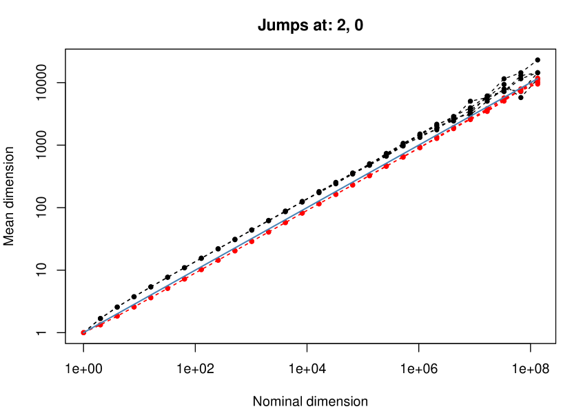
Figure 2: Computed mean dimension for $f(\boldsymbol{x})=1\{\theta^{\mathsf{T}}\boldsymbol{x}>t\}$, with $\theta_{j}=1/\sqrt{d}$ versus nominal dimension $d$. From top to bottom the thresholds are $t=2,0$. There were 5 independent computations with using $2^{20}$ scrambled Sobol’ points each. There is a reference line $y=\sqrt{d}$ in between the two sets of curves.

Figure 2 shows mean dimensions computed for $f(\boldsymbol{x})=1\{\sum_{j=1}^{d}x_{j}/\sqrt{d}>t\}$, a jump function, for $t\in\{2,0\}$. The mean dimension is the same for $t$ as for $-t$, so we do not include $t=-2$. All five replicates are plotted for each threshold; they overlap considerably for $d\leqslant 10^{6}$. For larger $d$, fluctuations are visible especially for $t=2$. The estimated mean dimensions are very nearly parallel to $\sqrt{d}$ over this range.

7 Conclusions

Integrands formed as ridge functions over Gaussian random variables $\boldsymbol{x}\sim\mathcal{N}(0,I)$ can have bounded mean dimension as the nominal dimension increases. It suffices for them to be Lipschitz functions of $\theta^{\mathsf{T}}\boldsymbol{x}$ for a unit vector $\theta$.

Ridge functions are simple enough that they can be integrated directly via one dimensional quadrature, and in some cases, by closed form expressions, yielding good test functions. In applications, an integrand may be close to a ridge function without the user being aware of it. Constantine [3] finds that many functions in engineering applications are well approximated by ridge functions. Some of our findings are for specific functions such as $(\theta^{\mathsf{T}}\boldsymbol{x}-t)_{+}$ or $1\{\theta^{\mathsf{T}}\boldsymbol{x}>t\}$ and it remains to see how generally they apply to other kinks and jumps.

Suppose that $f$ is approximately a ridge function of low mean dimension. We write $f(\boldsymbol{x})=g(\theta^{\mathsf{T}}\boldsymbol{x})+\varepsilon(\boldsymbol{x})$. Then under scrambled net sampling, the MSE is

$$\mathrm{Var}\Biggl{(}\frac{1}{n}\sum_{i=1}^{n}\bigl{(}g(\theta^{\mathsf{T}}\boldsymbol{x}_{i})+\varepsilon(\boldsymbol{x}_{i})\bigr{)}\Biggr{)} \leqslant 2\mathrm{Var}\Biggl{(}\frac{1}{n}\sum_{i=1}^{n}g(\theta^{\mathsf{T}}\boldsymbol{x}_{i})\Biggr{)}+2\mathrm{Var}\Biggl{(}\frac{1}{n}\sum_{i=1}^{n}\varepsilon(\boldsymbol{x}_{i})\Biggr{)}$$

$$\leqslant 2\mathrm{Var}\Biggl{(}\frac{1}{n}\sum_{i=1}^{n}g(\theta^{\mathsf{T}}\boldsymbol{x}_{i})\Biggr{)}+2\Gamma\frac{\mathrm{Var}(\varepsilon(\boldsymbol{x}))}{n},$$

where $\Gamma$ is the largest gain coefficient [25]. The factor of $2$ is a conservative upper bound. The first term benefits from low mean dimension of ridge functions and the smoothing effect of the ANOVA.

In projection pursuit regression [7], a high dimensional function is approximated by a sum of a small number of ridge functions. Single layer (not deep) neural networks approximate a function by a linear combination of smooth ridge functions [4]. Historically those ridge functions were smooth CDFs like $g(y)=(1+\exp(-y))^{-1}$ and more recently the positive part function $g(y)=\max(y,0)$ also called a rectified linear unit (relu) has been prominent. Both of these $g(\cdot)$ are Lipschitz. Those models are often good approximations to real world phenomena. They are usually fit to noisy data but noise is not a critical part of them being a good fit.

Suppose now that $f(\boldsymbol{x})=\sum_{j=1}^{J}f_{j}(\boldsymbol{x})$, where $f_{1},\dots,f_{J-1}$ are ridge functions and $f_{J}$ is a residual function with a small mean square. Then under RQMC sampling $\mathrm{Var}(\hat{\mu})\leqslant J\sum_{j=1}^{J}\mathrm{Var}(\hat{\mu}_{j})$ where $\hat{\mu}_{j}$ is the average of $f_{j}(\boldsymbol{x}_{i})$ over an RQMC sample $\boldsymbol{x}_{i}$. The factor $J$ is extremely conservative as it allows for perfect correlations among all $J$ integration errors.

We have not addressed whether it is realistic to expect $g$ to remain constant as $d\to\infty$. A full discussion of that point is beyond the scope of this article. Instead we make a few remarks.

If we think of Brownian motion with $d$ time steps to time $T=1$ then under the standard construction, the end point is $B(T)=(1/\sqrt{d})\sum_{j=1}^{d}x_{j}$. In this instance making $\theta$ a unit vector is a good generalization of infill asymptotics and a function of $B(T)$ or $B(\lambda T)$ for $0<\lambda<1$ takes on the form $g(\theta^{\mathsf{T}}\boldsymbol{x})$ for $\|\theta\|=1$. If instead, we consider Brownian motion with $d$ time steps to time $T=d$ then under the standard construction, the endpoint is $B(T)=\sum_{j=1}^{d}x_{j}$. We might model that via $f(\boldsymbol{x})=g(\sqrt{d}\theta^{\mathsf{T}}\boldsymbol{x})$. Introducing $\sqrt{d}$ within $g(\cdot)$ multiplies any Lipschitz bound for $g$ by $\sqrt{d}$ and then raises the upper bound on $\sum_{j}\overline{\tau}_{j}^{2}$ by a factor of $d$. Whatever effect this has on $\nu(f)$ depends on how introducing $\sqrt{d}$ within $g(\cdot)$ affects $\sigma^{2}$, the variance of $f$. The variance might also increase by a factor of $d$, leaving the mean dimension invariant to $d$. For instance, that would happen for $f(\boldsymbol{x})=(\sum_{j}x_{j}-t)_{+}$. If instead the variance remains remains nearly constant, then the mean dimension could grow with $d$. For instance if $f(\boldsymbol{x})=\Phi(\sum_{j}x_{j})$, then for large $d$ it is like a Heaviside function applied to $(1/\sqrt{d})\sum_{j}x_{j}$ and the mean dimension will grow like $\sqrt{d}$.

8 Appendix

8.1 Upper bound for jumps

Proof 8.1.

Here we prove Theorem 4.1. If $\theta_{k}=0$ then $\overline{\tau}^{2}_{k}=0$ too. We may suppose that any such $x_{k}$ have been removed from the model. Then

$$\overline{\tau}^{2}_{k} =\frac{1}{2}\mathbb{E}\Bigl{(}\bigl{(}1\{y+x>t\}-1\{y+z>t\}\bigr{)}^{2}\Bigr{)}$$

$$=\frac{1}{2}\mathbb{E}\Bigl{(}|1\{y+x>t\}-1\{y+z>t\}|\Bigr{)}$$

where $y\sim\mathcal{N}(0,1-\theta_{k}^{2})$ and $x,z\sim\mathcal{N}(0,\theta_{k}^{2})$ are all independent. Next, for any $\epsilon>0$

$$2\overline{\tau}^{2}_{k} \leqslant\Pr(|y+x-t|<\epsilon)+\Pr(|z-x|>\epsilon)$$

$$=\Phi(-t+\epsilon)-\Phi(-t-\epsilon)+2\Phi\Bigl{(}\frac{-\epsilon}{\sqrt{2}|\theta_{k}|}\Bigr{)}.$$

As a result

$$\nu(f) \leqslant\frac{1}{2\Phi(t)\Phi(-t)}\sum_{j=1}^{d}\Phi(-t+\epsilon_{k})-\Phi(-t-\epsilon_{k})+2\Phi\Bigl{(}\frac{-\epsilon_{k}}{\sqrt{2}|\theta_{k}|}\Bigr{)}.$$

Taking $\epsilon_{k}=\eta|\theta_{k}|$,

$$\nu(f) \leqslant\frac{1}{2\Phi(t)\Phi(-t)}\biggl{(}2d\Phi\Bigl{(}-\frac{\eta}{\sqrt{2}}\Bigr{)}+\sum_{j=1}^{d}\Phi(-t+\eta|\theta_{k}|)-\Phi(-t-\eta|\theta_{k}|)\biggr{)}$$

$$\leqslant\frac{1}{\Phi(t)\Phi(-t)}\biggl{(}\frac{d}{\eta/\sqrt{2}}\varphi\Bigl{(}-\frac{\eta}{\sqrt{2}}\Bigr{)}+\eta\varphi(0)\|\theta\|_{1}\biggr{)}$$

$$\leqslant\frac{1}{\Phi(t)\Phi(-t)\sqrt{2\pi}}\biggl{(}\frac{\sqrt{2}d}{\eta}\exp\Bigl{(}-\frac{\eta^{2}}{4}\Bigr{)}+\eta\|\theta\|_{1}\biggr{)}.$$

Choosing $\eta=2\sqrt{\log(d/\|\theta\|_{1})}$,

$$\nu(f) \leqslant\frac{\|\theta\|_{1}}{\Phi(t)\Phi(-t)\sqrt{2\pi}}\Bigl{(}\frac{\sqrt{2}}{\eta}+\eta\Bigr{)}$$

To conclude, $1\leqslant\|\theta\|_{1}\leqslant\sqrt{d}$, so for $d\geqslant 2$, $\eta\geqslant 2\sqrt{\log(2/\sqrt{2})}>1$.

8.2 A bivariate Gaussian probability lower bound

Proof 8.2.

Here we prove Lemma 4.5. For $\eta>0$,

$$\phantom{\geqslant}\ \Pr(x>t,y<t)$$

$$\geqslant\Pr(x>t+\eta,y<t-\eta)$$

$$=\frac{1}{2\pi(1-\rho^{2})^{1/2}}\int_{t}^{t+\eta}\int_{t-\eta}^{t}\exp\Bigl{(}-\frac{1}{2}[y_{1}^{2}-2\rho y_{1}y_{2}+y_{2}^{2}]/(1-\rho^{2})\Bigr{)}\,\mathrm{d}y_{2}\,\mathrm{d}y_{1}$$

$$\geqslant\frac{\eta^{2}}{2\pi(1-\rho^{2})^{1/2}}\exp\Bigl{(}-\frac{1}{2}[(t_{1}+\eta)^{2}-2\rho(t_{1}+\eta)(t_{2}-\eta)+(t_{2}-\eta)^{2}]/(1-\rho^{2})\Bigr{)},$$

because with $\rho\geqslant 0$ and $t\geqslant 0$, the bivariate normal probability density function is minimized over $[t,t+\eta]\times[t-\eta,t]$ at $(t+\eta,t-\eta)$. Simplifying this expression and then choosing $\eta=\sqrt{1-\rho}$,

$$\Pr(x>t,y<t) \geqslant\frac{\eta^{2}}{2\pi(1-\rho^{2})^{1/2}}\exp\Bigl{(}-\frac{t^{2}}{1+\rho}-\frac{\eta^{2}}{1-\rho}\Bigr{)}$$

$$=\frac{1}{2\pi}\Bigl{(}\frac{1-\rho}{1+\rho}\Bigr{)}^{1/2}\exp\Bigl{(}-\frac{t^{2}}{1+\rho}-1\Bigr{)}.$$

8.3 Lower bound for jumps

Proof 8.3.

Here we prove Theorem 4.3. Letting $y_{1}=\theta^{\mathsf{T}}\boldsymbol{x}$ and $y_{2}=x+\theta_{j}(z_{j}-x_{j})$ we get

$$\begin{pmatrix}y_{1}\\ y_{2}\end{pmatrix}\sim\mathcal{N}\biggl{(}\begin{pmatrix}0\\ 0\end{pmatrix},\begin{pmatrix}1&\rho_{j}\\ \rho_{j}&1\end{pmatrix}\biggr{)},\quad\text{for $\rho_{j}=1-\theta_{j}^{2}.$}$$

Now $\overline{\tau}^{2}_{j}=\Pr(y_{1}>t,y_{2}<t)$. From Lemma 4.5.

$$\overline{\tau}^{2}_{j} \geqslant\frac{1}{2\pi}\Bigl{(}\frac{1-\rho_{j}}{1+\rho_{j}}\Bigr{)}^{1/2}\exp\Bigl{(}-\frac{t^{2}}{1+\rho_{j}}-1\Bigr{)}$$

$$=\frac{1}{2\pi}\frac{|\theta_{j}|}{(2-\theta_{j}^{2})^{1/2}}\exp\Bigl{(}-\frac{t^{2}}{2-\theta_{j}^{2}}-1\Bigr{)}$$

$$\geqslant\frac{|\theta_{j}|}{2^{3/2}\pi}\exp(-t^{2}-1).$$

Summing over $j\in 1{:}d$ and dividing by $\sigma^{2}=\Phi(t)\Phi(-t)$ completes the proof.

8.4 Upper bound for kinks

Proof 8.4.

Here we prove Theorem 4.7. First for $j\in 1{:}d$,

$$\int_{0}^{1}f_{d,p}(\boldsymbol{x})\,\mathrm{d}x_{j} =\frac{1}{p+1}f_{d-1,p+1}(\boldsymbol{x}_{-j}).$$

Applying this result $|u|$ times, for $u\subsetneq 1{:}d$, yields

(21) $$\int_{[0,1]^{|u|}}f_{d,p}(\boldsymbol{x})\,\mathrm{d}x_{u} =\frac{\Gamma(p+1)}{\Gamma(p+|u|+1)}f_{d-|u|,p+|u|}(\boldsymbol{x}_{-u}).$$

Applying (21) formally for $u=1{:}d$ gives

$$\mu_{d,p}\equiv\int_{[0,1]^{d}}f_{d,p}(\boldsymbol{x})\,\mathrm{d}\boldsymbol{x}=\frac{\Gamma(p+1)}{\Gamma(p+d+1)}f_{0,p+d}(\boldsymbol{x}_{\varnothing}).$$

We can find more rigorously that

$$\mu_{d,p} =\int_{0}^{1}\frac{\Gamma(p+1)}{\Gamma(p+d)}f_{1,p+d-1}(x_{d})\,\mathrm{d}x_{d}=\frac{\Gamma(p+1)}{\Gamma(p+d)}\int_{0}^{1}x^{p+d-1}\,\mathrm{d}x=\frac{\Gamma(p+1)}{\Gamma(p+d+1)},$$

and so we get the correct answer from a convention that $f_{0,p+d}(\boldsymbol{x}_{\varnothing})=1$. The variance of $f_{d,p}$ is

$$\sigma^{2}_{d,p}=\mu_{d,2p}-\mu_{d,p}^{2}=\frac{\Gamma(2p+1)}{\Gamma(2p+d+1)}-\Bigl{(}\frac{\Gamma(p+1)}{\Gamma(p+d+1)}\Bigr{)}^{2}.$$

For $f_{d,p}$, we get a Sobol’ index of

$$\overline{\tau}^{2}_{d} =\frac{1}{2}\int\biggl{(}f_{d,p}(\boldsymbol{x})-\Bigl{(}z_{d}+\sum_{j=1}^{d-1}x_{j}-(d-1)\Bigr{)}_{+}^{p}\,\mathrm{d}\boldsymbol{x}\,\mathrm{d}z_{d}\biggr{)}^{2}$$

$$=\mu_{d,2p}-\int f_{d,p}(\boldsymbol{x})\Bigl{(}z_{d}+\sum_{j=1}^{d-1}x_{j}-(d-1)\Bigr{)}_{+}^{p}\,\mathrm{d}\boldsymbol{x}\,\mathrm{d}z_{d}$$

$$=\mu_{d,2p}-\Bigl{(}\frac{\Gamma(p+1)}{\Gamma(p+2)}\Bigr{)}^{2}\int f_{d-1,p+1}(\boldsymbol{x}_{-d})^{2}\,\mathrm{d}\boldsymbol{x}_{-d}$$

$$=\mu_{d,2p}-\Bigl{(}\frac{\Gamma(p+1)}{\Gamma(p+2)}\Bigr{)}^{2}\mu_{d-1,2p+2}$$

$$=\frac{\Gamma(2p+1)}{\Gamma(2p+d+1)}-\Bigl{(}\frac{\Gamma(p+1)}{\Gamma(p+2)}\Bigr{)}^{2}\frac{\Gamma(2p+3)}{\Gamma(2p+d+2)}.$$

Now because $\overline{\tau}^{2}_{j}=\overline{\tau}^{2}_{d}$ by symmetry for all $j\in 1{:}d$, we get

$$\nu(f_{d,p}) =\frac{d\Bigl{(}\frac{\Gamma(2p+1)}{\Gamma(2p+d+1)}-\bigl{(}\frac{\Gamma(p+1)}{\Gamma(p+2)}\bigr{)}^{2}\frac{\Gamma(2p+3)}{\Gamma(2p+d+2)}\Bigr{)}}{\frac{\Gamma(2p+1)}{\Gamma(2p+d+1)}-\bigl{(}\frac{\Gamma(p+1)}{\Gamma(p+d+1)}\bigr{)}^{2}}.$$

8.5 Mean dimension of preintegrated step functions

Proof 8.5.

Here we prove Theorem 5.3. We will use

(22) $$\int_{-\infty}^{\infty}\Phi(a+bx)\varphi(x)\,\mathrm{d}x =\Phi\biggl{(}\frac{a}{\sqrt{1+b^{2}}}\biggr{)},\quad\text{and}$$

(23) $$\int_{-\infty}^{\infty}\Phi(a+bx)^{2}\varphi(x)\,\mathrm{d}x =\Phi\biggl{(}\frac{a}{\sqrt{1+b^{2}}}\biggr{)}-2T\biggl{(}\frac{a}{\sqrt{1+b^{2}}},\frac{1}{\sqrt{1+2b^{2}}}\biggr{)},\quad\text{where}$$

$$T(h,a) =\varphi(h)\int_{0}^{a}\frac{\varphi(hx)}{1+x^{2}}\,\mathrm{d}x.$$

These are formulas 10,010.8 and 20,010.4, respectively, from [29].

Recalling that $\theta_{\ell}\neq 0$,

$$\bar{f}_{\ell}(\boldsymbol{x})=\Phi\biggl{(}\frac{(1-\theta_{\ell}^{2})^{1/2}\theta^{*\mathsf{T}}_{\ell}\boldsymbol{x}-t}{\theta_{\ell}}\biggr{)}=\Phi\biggl{(}\frac{\sum_{k\neq\ell}\theta_{k}x_{k}-t}{\theta_{\ell}}\biggr{)}$$

So for $j\neq\ell$, letting $\gamma_{j}=\sqrt{1-\theta_{j}^{2}-\theta_{\ell}^{2}}$,

$$\overline{\tau}^{2}_{j} =\frac{1}{2}\mathbb{E}\Biggl{(}\biggl{[}\Phi\biggl{(}\frac{\gamma_{j}y_{j}+\theta_{j}x_{j}-t}{\theta_{\ell}}\biggr{)}-\Phi\biggl{(}\frac{\gamma_{j}y_{j}+\theta_{j}z_{j}-t}{\theta_{\ell}}\biggr{)}\biggr{]}^{2}\Biggr{)}$$

$$=\mathbb{E}\bigl{(}\bar{f}_{\ell}(\boldsymbol{x})^{2}\bigr{)}-\mathbb{E}\biggl{(}\Phi\biggl{(}\frac{\gamma_{j}y_{j}+\theta_{j}x_{j}-t}{\theta_{\ell}}\biggr{)}\Phi\biggl{(}\frac{\gamma_{j}y_{j}+\theta_{j}z_{j}-t}{\theta_{\ell}}\biggr{)}\biggr{)},$$

where $x_{j},y_{j},z_{j}$ are independent $\mathcal{N}(0,1)$ random variables.

First, from (23)

$$\mathbb{E}\bigl{(}\bar{f}_{\ell}(\boldsymbol{x})^{2}\bigr{)} =\int_{-\infty}^{\infty}\Phi\biggl{(}\frac{(1-\theta_{\ell}^{2})^{1/2}z-t}{\theta_{\ell}}\biggr{)}^{2}\,\mathrm{d}z=\Phi\bigl{(}-t\bigr{)}-2T\biggl{(}-t,\frac{\theta_{\ell}}{(2-\theta_{\ell}^{2})^{1/2}}\biggr{)}.$$

Next, applying (22) to $x_{j}$ and $z_{j}$, followed by (23) to $y_{j}$

$$\mathbb{E}\biggl{(}\Phi\biggl{(}\frac{\gamma_{j}y_{j}+\theta_{j}x_{j}-t}{\theta_{\ell}}\biggr{)}\Phi\biggl{(}\frac{\gamma_{j}y_{j}+\theta_{j}z_{j}-t}{\theta_{\ell}}\biggr{)}\biggr{)}$$

$$=\mathbb{E}\biggl{(}\Phi\biggl{(}\frac{\gamma_{j}y_{j}-t}{(\theta_{j}^{2}+\theta_{\ell}^{2})^{1/2}}\biggr{)}^{2}\biggr{)}$$

$$=\Phi\bigl{(}-t\bigr{)}-2T\biggl{(}-t,\frac{(\theta_{j}^{2}+\theta_{\ell}^{2})^{1/2}}{(2-\theta_{j}^{2}-\theta_{\ell}^{2})^{1/2}}\biggr{)}.$$

Recalling $a_{1}=\theta_{\ell}/(2-\theta_{\ell}^{2})^{1/2}$ and $a_{2}=a_{2}(j)=(\theta_{j}^{2}+\theta_{\ell}^{2})^{1/2}/(2-\theta_{j}^{2}-\theta_{\ell}^{2})^{1/2}$, so

$$\overline{\tau}^{2}_{j} =2T\biggl{(}-t,\frac{(\theta_{j}^{2}+\theta_{\ell}^{2})^{1/2}}{(2-\theta_{j}^{2}-\theta_{\ell}^{2})^{1/2}}\biggr{)}-2T\biggl{(}-t,\frac{\theta_{\ell}}{(2-\theta_{\ell}^{2})^{1/2}}\biggr{)}=2\varphi(t)\int_{a_{1}}^{a_{2}}\frac{\varphi(tx)}{1+x^{2}}\,\mathrm{d}x.$$

The variance of $\bar{f}_{\ell}$ is

$$\sigma^{2} =\Phi(-t)-2T\biggl{(}-t,\frac{\theta_{\ell}}{(2-\theta_{\ell}^{2})^{1/2}}\biggr{)}-\Phi(-t)^{2}$$

$$=\Phi(t)\Phi(-t)-2\varphi(t)\int_{0}^{a_{1}}\frac{\varphi(tx)}{1+x^{2}}\,\mathrm{d}x,$$

and so

$$\nu(\bar{f}_{\ell})=\frac{2\varphi(t)\sum_{j\neq\ell}\int_{a_{1}}^{a_{2}(j)}\frac{\varphi(tx)}{1+x^{2}}\,\mathrm{d}x}{\Phi(t)\Phi(-t)-2\varphi(t)\int_{0}^{a_{1}}\frac{\varphi(tx)}{1+x^{2}}\,\mathrm{d}x}$$

establishing (18). For $t=0$,

$$\nu(\bar{f}_{\ell}) =\frac{\pi^{-1}\sum_{j\neq\ell}\int_{a_{1}}^{a_{2}(j)}(1+x^{2})^{-1}\,\mathrm{d}x}{1/4-\pi^{-1}\int_{0}^{a_{1}}(1+x^{2})^{-1}\,\mathrm{d}x}=\frac{\sum_{j\neq\ell}\bigl{(}\tan^{-1}(a_{2}(j))-\tan^{-1}(a_{1})\bigr{)}}{\pi/4-\tan^{-1}(a_{1})},$$

establishing (19). Finally, if $\theta_{\ell}=\theta_{j}=1/\sqrt{d}$, then $a_{1}=(2d-1)^{-1/2}$ and $a_{2}=(d-1)^{-1/2}$ and so

$$\nu(\bar{f}_{\ell}) =\frac{(d-1)[\tan^{-1}((d-1)^{-1/2})-\tan^{-1}((2d-1)^{-1/2})]}{\pi/4-\tan^{-1}((d-1)^{-1/2})}$$

$$=\frac{(d-1)[d^{-1/2}+O(d^{-3/2})-(2d)^{-1/2}+O(d^{-3/2})]}{\pi/4-O(d^{-1/2})},$$

establishing (20).

References

- [1] H.-J. Bungartz and M. Griebel, Sparse grids, Acta numerica, 13 (2004), pp. 147–269.
- [2] R. E. Caflisch, W. Morokoff, and A. B. Owen, Valuation of mortgage backed securities using Brownian bridges to reduce effective dimension, Journal of Computational Finance, 1 (1997), pp. 27–46.
- [3] P. G. Constantine, Active subspaces: Emerging ideas for dimension reduction in parameter studies, SIAM, Philadelphia, 2015.
- [4] G. Cybenko, Approximation by superpositions of a sigmoidal function, Mathematics of control, signals and systems, 2 (1989), pp. 303–314.
- [5] J. Dick and F. Pillichshammer, Digital sequences, discrepancy and quasi-Monte Carlo integration, Cambridge University Press, Cambridge, 2010.
- [6] B. Efron and C. Stein, The jackknife estimate of variance, Annals of Statistics, 9 (1981), pp. 586–596.
- [7] J. H. Friedman and W. Stuetzle, Projection pursuit regression, Journal of the American statistical Association, 76 (1981), pp. 817–823.
- [8] P. G. Glasserman, Monte Carlo methods in financial engineering, Springer, New York, 2004.
- [9] M. Griebel, F. Y. Kuo, and I. H. Sloan, The smoothing effect of the ANOVA decomposition, Journal of Complexity, 26 (2010), pp. 523–551.
- [10] M. Griebel, F. Y. Kuo, and I. H. Sloan, The smoothing effect of integration in and the ANOVA decomposition, Mathematics of Computation, 82 (2013), pp. 383–400.
- [11] M. Griebel, F. Y. Kuo, and I. H. Sloan, Note on “The smoothing effect of integration in and the ANOVA decomposition”, Mathematics of Computation, 86 (2017), pp. 1847–1854.
- [12] A. Griewank, F. Y. Kuo, H. Leövey, and I. H. Sloan, High dimensional integration of kinks and jumps—Smoothing by preintegration, Journal of Computational and Applied Mathematics, 344 (2018), pp. 259–274.
- [13] Z. He and X. Wang, On the convergence rate of randomized quasi–Monte Carlo for discontinuous functions, SIAM Journal on Numerical Analysis, 53 (2015), pp. 2488–2503.
- [14] F. J. Hickernell, Koksma-Hlawka inequality, Wiley StatsRef: Statistics Reference Online, (2014).
- [15] W. Hoeffding, A class of statistics with asymptotically normal distribution, Annals of Mathematical Statistics, 19 (1948), pp. 293–325.
- [16] S. Joe and F. Y. Kuo, Constructing Sobol’ sequences with better two-dimensional projections, SIAM Journal on Scientific Computing, 30 (2008), pp. 2635–2654.
- [17] F. Kuo, I. Sloan, G. Wasilkowski, and H. Woźniakowski, On decompositions of multivariate functions, Mathematics of computation, 79 (2010), pp. 953–966.
- [18] F. Y. Kuo and D. Nuyens, Application of quasi-Monte Carlo methods to elliptic PDEs with random diffusion coefficients: a survey of analysis and implementation, Foundations of Computational Mathematics, 16 (2016), pp. 1631–1696.
- [19] R. Liu and A. B. Owen, Estimating mean dimensionality of analysis of variance decompositions, Journal of the American Statistical Association, 101 (2006), pp. 712–721.
- [20] B. Moskowitz and R. E. Caflisch, Smoothness and dimension reduction in quasi-Monte Carlo methods, Mathematical and Computer Modelling, 23 (1996), pp. 37–54.
- [21] H. Niederreiter, Random Number Generation and Quasi-Monte Carlo Methods, SIAM, Philadelphia, PA, 1992.
- [22] A. Ostrowski, über normen von matrizen, Mathematische Zeitschrift, 63 (1955), pp. 2–18.
- [23] A. B. Owen, Randomly permuted -nets and -sequences, in Monte Carlo and Quasi-Monte Carlo Methods in Scientific Computing, H. Niederreiter and P. J.-S. Shiue, eds., New York, 1995, Springer-Verlag, pp. 299–317.
- [24] A. B. Owen, Monte Carlo variance of scrambled net quadrature, SIAM Journal of Numerical Analysis, 34 (1997), pp. 1884–1910.
- [25] A. B. Owen, Scrambling Sobol’ and Niederreiter-Xing points, Journal of Complexity, 14 (1998), pp. 466–489.
- [26] A. B. Owen, The dimension distribution and quadrature test functions, Statistica Sinica, (2003), pp. 1–17.
- [27] A. B. Owen, Multidimensional variation for quasi-Monte Carlo, in International Conference on Statistics in honour of Professor Kai-Tai Fang’s 65th birthday, J. Fan and G. Li, eds., 2005.
- [28] A. B. Owen, A randomized Halton algorithm in R, Tech. Report arXiv:1706.02808, Stanford University, 2017.
- [29] D. B. Owen, A table of normal integrals: A table, Communications in Statistics-Simulation and Computation, 9 (1980), pp. 389–419.
- [30] J. K. Patel and C. B. Read, Handbook of the normal distribution, vol. 150, Marcel Dekker, Inc., New York, 2nd ed., 1996.
- [31] I. H. Sloan and S. Joe, Lattice Methods for Multiple Integration, Oxford Science Publications, Oxford, 1994.
- [32] I. M. Sobol’, The distribution of points in a cube and the accurate evaluation of integrals, USSR Computational Mathematics and Mathematical Physics, 7 (1967), pp. 86–112.
- [33] I. M. Sobol’, Multidimensional Quadrature Formulas and Haar Functions, Nauka, Moscow, 1969. (In Russian).
- [34] I. M. Sobol’, Sensitivity estimates for nonlinear mathematical models, Mathematical Modeling and Computational Experiment, 1 (1993), pp. 407–414.
- [35] X. Wang, Improving the rejection sampling method in quasi-Monte Carlo methods, Journal of computational and applied Mathematics, 114 (2000), pp. 231–246.
- [36] G. Wasilkowski, -superposition and truncation dimensions and multivariate decomposition method for -variate linear problems, in Multivariate Algorithms and Information-Based Complexity, F. J. Hickernell and P. Kritzer, eds., Berlin/Boston, 2019, De Gruyter. Accepted.
- [37] A. Winkelbauer, Moments and absolute moments of the normal distribution, Tech. Report arXiv:1209.4340, Vienna University of Technology, 2012.