Phase Separation and Exotic Vortex Phases in a Two-Species Holographic Superfluid

Abstract

At a finite temperature, the stable equilibrium states of a coupled two-component superfluid with the same mass in both non-rotating and rotating cases can be obtained by studying its real time dynamics via holography, the equilibrium state is the final stable state that does not change in time anymore in the evolution process . Without rotation, the spatial phase separated states of the two components become more stable than the miscible condensates state when the direct repulsive inter-component coupling constant $\eta>\eta_{c}=0.05$ when the Josephson coupling $\epsilon$ is turned off. While a finite $\epsilon$ will always prevent the two species to be separated spatially. Under rotation, with vanishing $\epsilon$, the quantum fluid reveals many equilibrium structures of vortex states by varying the $\eta$ from negative to positive, the interlaced vortex lattices undergo a phase transition to vortex sheets with each component made up of chains of single quantized vortices.

I Introduction

The gauge-gravity dualityMaldacena ; Witten ; Gubser that relates strongly interacting quantum field theories to theories of classic gravity in higher dimensions has provided a new scheme not only to study strongly interacting condensed matter systems in equilibriumZaanen:2015oix ; Ammon2015 , but also to study the real time dynamics when the system is far away from equilibrium Liu:2018crr ; Liu ; Sonner:2014tca ; Bhaseen ; Chesler:2014gya . The first proposed theory of a single component holographic superfluid/BEC was given in Gubser2008 ; Hartnoll ; Herzog . The array of vortices is known to happen in a rotating superfluidFeynman . To find a static vortex lattice solution in the presence of rotation without studying the dynamic process in holography is always very hard technically, an only single vortex has been obtained in the single component system in Montull ; Domenech ; Keranen ; Maeda ; Dias ; Tallarita . However, by studying the full dynamics of the single component holographic superfluid/BEC in a rotating disk, the equilibrium vortex lattice can be obtained as the final time independent solutions in the real time dynamics process Xia:2019eje ; Tianyu , Besides the superfluid/BEC with only one order parameter, a two-component superfluids/BECs with two coupled order parameters has also become one of the most concerned topics in condensed matter physics, since it demonstrates novel quantum states that can not be observed in a single component system as predicted in the frame work of two component Gross-Pitaevskii (G-P) equationsKasamatsu-review . The two components $\Psi_{1}$ and $\Psi_{2}$ are coupled through a direct coupling term $\eta|\Psi_{1}|^{2}|\Psi_{2}|^{2}$ and a Josephson coupling $\epsilon(\Psi_{1}\Psi_{2}^{*}+\Psi_{1}^{*}\Psi_{2})$. Without rotation, a two-component BECs will enter a spatial separation state for the two order parameters due to the repulsive interaction $\eta>0$ between the two componentsShenoy ; Bohn ; Timmermans ; Cornell . In the presence of rotation, by solving the time dependent two-component G-P equation, the equilibrium vortex structures can be obtained after a sufficient long time revolution, which reveal rich structures by varying the direct coupling between the two components. As $\eta$ increase the interlocked vortex lattices undergo phase transitions from triangular to square, to double-core lattices, and eventually develop vortex sheetsUeda ; Kasamatsu . Vortex sheet is a state that the vortices are aligned to make up winding chains of single quantized vortices, and the chains of two components are interwoven alternately, or form as the cylindrical vortex sheets. Such a solution was proposed for the first time by Landau and Lifshitz Landau and has been observed experimentally in ³He AParts . Vortex sheet has proved to be an important physical object with nontrivial topology, which has many physical applicationsVolovik .

The purpose of this article is to research the equilibrium state properties of a strongly coupled two component BECs both in the presence of rotation and without rotation by using the holographic method. The static equilibrium states are calculated from the time dependent evolution equations, where the static solution can be obtained by evolving the system from an initial homogeneous superfluid state in the presence of a perturbation induced by rotation or a small fluctuation. Our treatment is very similar to the calculation in the frame of a time dependent two component G-P equation, where the static solution was found as the final state that does not change in time anymoreUeda ; Kasamatsu . When there is no rotation, the phase separation states was studied in detail for different temperatures and different values of coupling constant. We found that the phase separation states prefer to appear at lower temperature with a relatively higher inter-components direct repulsive interaction, while the Josephson coupling is always prevent the system to be phase separated. Under rotation, the holographic superfluid reveals four structures of vortex states corresponding different values of direct coupling between the two components by turning off the Josephson coupling. The four structures include a triangle lattice, a square lattice, a vortex stripe and a vortex sheet, the vortex sheet solution is a result of phase separation. The vortex diagram in the intercomponent direct coupling $\eta$ versus rotation-frequency $\Omega$ is also calculated, which is similar to the one obtained from the two component (G-P) equations Kasamatsu . Because of the nonlinear nature of the gravity theory, we will have to rely on numerical methods by solving a highly nonlinear partial differential gravity equations.

This paper is organized as follows. Section 2 introduces the holographic $U(1)$ symmetry broken model with two order parameters, the equations of motion (EoMs) for the model and also the numerical method we adapted to solve the EoMs. Section 3 discusses the properties of the two component system without rotation and the phase separation state is obtained with a large repulsive inter-components coupling. Section 4 presents the appearance of exotic vortex phases of the two-component system under rotation, and the vortex phase diagram is also obtained. Section 5 is devoted to the conclusion and some discussions.

II Holographic model and the time evolution equations of motion

The holographic model we use is a bottom-up construction containing two coupled charged scalar fields living in an $AdS$ black hole background, which is an direct extension of the single component holographic superfluid model proposed in Hartnoll . The action includes two charged scalar fields that coupled to a $U(1)$ gauge fieldWen:2013ufa

$$S=\int d^{4}x\sqrt{-g}\Big{[}-\frac{1}{4}F^{2}-\sum_{j=1}^{2}(|D\Psi_{j}|^{2}-m_{j}^{2}|\Psi_{j}|^{2})+V(\Psi_{1},\Psi_{2})\Big{]},$$ (1)

the inter-component coupling potential between the two charged scalar fields takes the form

$$V(\Psi_{1},\Psi_{2})=\epsilon(\Psi_{1}\Psi_{2}^{*}+\Psi_{1}^{*}\Psi_{2})+\eta|\Psi_{1}|^{2}|\Psi_{2}|^{2},$$ (2)

where $\eta$ is called the direct coupling while $\epsilon$ is the Josephson coupling. Note that the interaction potential takes the same form as the G-P equations for a coupled two component superfluid Ueda ; Galteland ; Nitta . In the holography, there is another more complex model dual to a two component superfluid with two gauge fields coupled to two charged scalar fields respectively Bigazzi:2011ak ; Musso .

Also in the action, $F_{\mu\nu}=\partial_{\mu}A_{\nu}-\partial_{\nu}A_{\mu}$, $D_{\mu}=\partial_{\mu}-iqA_{\mu}$ with $q$ the charge. The metric of the $AdS_{4}$ black hole background in the Eddington-Finkelstein coordinates reads

$$ds^{2}=\frac{\ell^{2}}{z^{2}}\left(-f(z)dt^{2}-2dtdz+dr^{2}+r^{2}d\theta^{2}\right).$$ (3)

in which $\ell$ is the AdS radius, $z$ is the AdS radial coordinate of the bulk and $f(z)=1-(z/z_{h})^{3}$. Thus, $z=0$ is the AdS boundary while $z=z_{h}$ is the horizon; the Hawking temperature is $T=3/(4\pi z_{h})$. $r$ and $\theta$ are respectively the radial and angular coordinates of the dual $2+1$ dimensional boundary, which is a disk that suitable to study the properties of the two component superfluid under rotation.

The axial gauge $A_{z}=0$ is adopted as in Liu ; Herzog . Near the boundary $z=0$, by choosing that $m_{1}^{2}=m_{2}^{2}=-2$, the general solutions take the asymptotic form as,

$$A_{\nu} = a_{\nu}+b_{\nu}z+\mathcal{O}(z^{2}),$$ (4)

$$\Psi_{j} = \Psi_{j}^{1}z+\Psi_{j}^{2}z^{2}+\mathcal{O}(z^{3}).$$ (5)

$j=1,2$, the coefficients $a_{r,\theta}$ can be regarded as the superfluid velocity along $r,\theta$ directions while $b_{r,\theta}$ as the conjugate currents Montull . Coefficients $a_{t}$ and $b_{t}$ areinterpreted as chemical potential $\mu$ and charge density $\rho$ respectively in the boundary field theory. Moreover, $\Psi_{j}^{1}$ is a source term which is set to be zero, then $\Psi_{j}^{2}$ is the vacuum expectation value $\langle O_{j}\rangle$ of the dual scalar operator in the boundary in the spontaneous symmetry broken phase. Without loss of generality we rescale $\ell=z_{h}=q=1$. Therefore, by scaling $\Psi_{j}=\psi_{j}z$ and using the axial gauge that $A_{z}=0$, the equations of motion (EoMs) can be written as

$$\begin{split}\partial_{t}\partial_{z}\psi_{1}=\frac{1}{2}\{-\epsilon\frac{\psi_{2}}{z^{2}}-\eta\psi_{1}|\psi_{2}|^{2}+i[\psi_{1}\partial_{z}A_{t}+2A_{t}\partial_{z}\psi_{1}-\psi_{1}\partial_{r}A_{r}+2A_{r}\partial_{r}\psi_{1}-\frac{\psi_{1}\partial_{\theta}A_{\theta}+2A_{\theta}\partial_{\theta}\psi_{1}}{r^{2}}]\\ +[(1-z^{3})\partial_{z}^{2}-3z^{2}\partial_{z}+\partial_{r}^{2}+\frac{\partial_{\theta}^{2}}{r^{2}}-z-A_{r}^{2}-\frac{A_{\theta}^{2}}{r^{2}}]\psi_{1}\},\end{split}$$ (6)

$$\begin{split}\partial_{t}\partial_{z}\psi_{2}=\frac{1}{2}\{-\epsilon\frac{\psi_{1}}{z^{2}}-\eta\psi_{2}|\psi_{1}|^{2}+i[\psi_{2}\partial_{z}A_{t}+2A_{t}\partial_{z}\psi_{2}-\psi_{2}\partial_{r}A_{r}+2A_{r}\partial_{r}\psi_{2}-\frac{\psi_{2}\partial_{\theta}A_{\theta}+2A_{\theta}\partial_{\theta}\psi_{2}}{r^{2}}]\\ +[(1-z^{3})\partial_{z}^{2}-3z^{2}\partial_{z}+\partial_{r}^{2}+\frac{\partial_{\theta}^{2}}{r^{2}}-z-A_{r}^{2}-\frac{A_{\theta}^{2}}{r^{2}}]\psi_{2}\},\end{split}$$ (7)

$$\partial_{z}^{2}A_{t}=-2\Im(\psi_{1}^{*}\partial_{z}\psi_{1}+\psi_{2}^{*}\partial_{z}\psi_{2})+\partial_{z}\partial_{r}A_{r}+\frac{\partial_{z}\partial_{\theta}A_{\theta}}{r^{2}},$$ (8)

$$\partial_{t}\partial_{z}A_{r}=\Im(\psi_{1}^{*}\partial_{r}\psi_{1}+\psi_{2}^{*}\partial_{r}\psi_{2})-A_{r}(|\psi_{1}|^{2}+|\psi_{2}|^{2})+\frac{\partial_{z}\partial_{r}A_{t}}{2}+\frac{\partial_{\theta}^{2}A_{r}-\partial_{r}\partial_{\theta}A_{\theta}}{2r^{2}}+\frac{(1-z^{3})\partial_{z}^{2}-3\partial_{z}}{2}A_{r},$$ (9)

$$\partial_{t}\partial_{z}A_{\theta}=\Im(\psi_{1}^{*}\partial_{\theta}\psi_{1}+\psi_{2}^{*}\partial_{\theta}\psi_{2})-A_{\theta}(|\psi_{1}|^{2}+|\psi_{2}|^{2})+\frac{\partial_{r}\partial_{\theta}A_{r}-\partial_{r}^{2}A_{\theta}+\partial_{z}\partial_{\theta}A_{t}}{2}+\frac{(1-z^{3})\partial_{z}^{2}-3\partial_{z}}{2}A_{\theta}.$$ (10)

The rotation is introduced by imposing the angular boundary condition as Domenech

$$a_{\theta}=\Omega r^{2},$$ (11)

where $\Omega$ is the constant angular velocity of the disk. The radius of the boundary disk is set as $r=R$. The Neumann boundary conditions are adopted both at $r=R$ and $r=0$, $\partial_{r}h_{i}=0$ where $h_{i}$ represents all the fields except $a_{\theta}$.

The EoMs are solved numerically by the Chebyshev spectral method in the $z,r$ direction, while Fourier decomposition is adopted in the $\theta$ direction. The time evolution is simulated by the fourth order Runge-Kutta method. The GPU Computing is used to speed up the calculation. The initial state at $t=0$ is always chosen to be a homogeneous solution for fixed ($\epsilon,\eta$) when there is no rotation, which can be obtained by solving the time independent EoMs by fixing a charge density $\rho$ with the Newton-Raphson method. Such an initial homogeneous state will evolve by perturbing the system with the rotation. The confiration after a long time revolution is considered to be stable when the changes of the norm of all fields become smaller than $10^{-5}$ for sufficient long time. Practically, a solutions at later time $t$ is used to minus the solutions at $t-\delta t$, when the maximum of the change of the solution become smaller than $10^{-5}$ for sufficient long time (for example $\delta t=100$), then the solution can be though to be a stable one. We also check that the solution satisfies the equations of motion with errors less than $10^{-5}$. Stay in the homogeneous ansartz, there is a critical $\rho_{c}(\epsilon,\eta)$ above which the two scalar fields will condense with the same value. From numerics we found that $\rho_{c}(0,0)\sim 4.07$, then the dimensionless critical temperature is $T_{c}^{0}=\frac{3}{4\pi\sqrt{\rho_{c}(0,0)}}=0.1183$. Turning on the direct coupling $\eta$ from $-0.5$ to $0.5$ will not alter the critical temperature, though a positive/negative $\eta$ will reduce/increase the value of order parameter a bit. By tuning $\epsilon$ from $0$ to $0.1$, the critical $\rho_{c}$ is decreasing, means the critical temperature is increasing, for example, the $\rho_{c}(0.1,0)=3.7$ indicates a higher $T_{c}=0.1241$. In all the dynamic simulation we set $T=0.82T_{c}^{0}$, at which for every combination of $-0.5\leq\eta\leq 0.5$ and $0\leq\epsilon\leq 0.1$, the system always have a stable homogeneous solution with the same finite value of order parameters for the two components.

III Phase separation in the presence of no rotation

Figure 1: (a)-(b) The overlap factor $\chi$ as a function of $\eta$. (c)-(d) The configuration of $\langle O_{1}(x)\rangle$(black line) and $\langle O_{2}(x)\rangle$(red line) in a phase separated phase.

Phase separation is an inhomogeneous solution that the two condensates do not overlap spatially. Such an immiscible state can be more stable with a lower free energy than the miscible state, which is a result of the repulsive interaction between the two condensations when the positive $\eta$ is large enough. The inhomogeneous stable solution can be obtained by solving the full time dependent equation. At initial time the system is also in a homogeneous and miscible solution with $\Psi_{1}=\Psi_{2}$ at fixed $\epsilon,\eta$, such a homogeneous state might be a metastable state which can evolve to a final stable inhomogeneous state by perturbing the system with a very small fluctuation, the real ground state. Without rotation, it is more convinient to adopt the Cartesian coordinate rather than the polar coordinate in the boundary theory, the metric is then $ds^{2}=\frac{\ell^{2}}{z^{2}}\left(-f(z)dt^{2}-2dtdz+dx^{2}+dy^{2}\right)$. To focus on the phase separation in the $x$ direction, we take the ansartz that all the fields are functions of $t,z,x$. To quantitatively describe the spatial overlap of the two condensations, we define an integral

$$\chi=\int_{0}^{L}dx\frac{|\langle O_{1}(x)\rangle||\langle O_{2}(x)\rangle|}{|\langle O_{h}\rangle|.^{2}},$$ (12)

where $\langle O_{h}\rangle$ is the corresponding homogeneous order parameter at $t=0$, the length $L=50$.

If $\chi=1$, system shows no phase separation, and it stays in the initial homogeneous state. Otherwise, if $\chi\ll 1$, it would be fair to say the system shows phase separation. In the intermediate case, the system is partially phase-separated and partially phase-mixed. In Fig. 1(a), we show the overlap integral $\chi$ as a function of $\eta$ at three different temperatures when $\epsilon=0$. The increase of $\chi$ along temperature when $\eta=0.5$ indicates that the system is harder to enter the phase separation phase, agrees with the increased correlation length of both condensations when $T$ is approaching $T_{c}$. In Figs. 1(b), the $\chi(\eta)$ is shown for three different $\epsilon$ at a fixed temperature, a small $\epsilon=0.01$ will increase the $\chi(\eta)$, indicates that the two condensations prefers to overlap spatially by increasing the Josephson coupling $\epsilon$. We also checked that in the case $\epsilon=0.1$, the system is always in the phase overlap state even in the strong repulsive interaction when $\eta=0.5$, $\chi$ is always to be one. Two samples of $\langle O_{1,2}\rangle$ of a separated phase with large repulsive interaction are illustrated in Fig.1 (c), and Fig.1 (d). Such an exotic immiscible state has been experimentally observed in a two-Hall and a three-Stenger component quantum fluid. Interesting, the phase separated state can also be obtained from a holographic first order phase transition in inhomogeneous black holesJanik ; Attems .

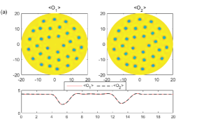
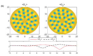
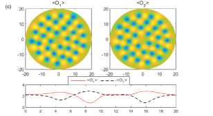
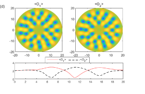
Figure 2: Four typical vortex phases at $T=0.82T_{c}^{0}$ and the corresponding radial profiles of $\langle O_{1,2}\rangle$ in the $\theta=\pi/2$ direction : (a) $\epsilon=0.1,\eta=0.1,\omega=0.1$. (b) $\epsilon=0,\eta=-0.6,\omega=0.1$. (c) $\epsilon=0,\eta=-0.2,\omega=0.1$. (d)$\epsilon=0,\eta=-0.05,\omega=0.1$.

IV exotic vortex phases under rotation and the phase diagram

In the section we move to the case that the system is in the presence of rotation, focusing on the case when the holographic two component superfluid is at a temperature $T=0.82T_{c}^{0}$. Several kinds of exotic vortex phases have been found. Firstly, since a finite $\epsilon=0.1$ will prevent the system to enter the phase separation state even $\eta$ is finite, then we expected that the vortices of the two components coincide, and a trianglar vortex lattice is expected as in the one component case Xia:2019eje . A sample result of $\epsilon=0.1$ and $\eta=0.1$ is shown in Fig.2 (a), even we increase $\eta$ to $0.5$. the vortices of both components have the same positions matches the two single vortices solution for the two components locate at the same position Wu . Since in the case of finite $\epsilon$, we will always find a configuration that the two component vortices take the same position, $\epsilon$ is set to be zero. Then by tuning the inter-component interaction $\eta$ from $-0.6$ to $0.6$, the system will demonstrate several exotic vortex phases. In Fig. 2 (b),(c) and (d), by increasing $\eta$ from $-0.6$ we see triangular lattices ($-0.6\leq\Omega\leq-0.45$), square lattices ($-0.45\leq\Omega\leq-0.1$) and vortex stripes ($-0.1<\Omega<0.05$). The square lattice is stable, presumably due to the fact that each vortex in one component can have all its nearest-neighbor vortices to be in the other componentSchweikhard .These various structures are similar to that obtained by the component G-P equations Kasamatsu .

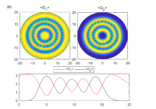
Figure 3: Two typical perfect vortex sheet solutions and the corresponding radial profiles of $\langle O_{1,2}\rangle$ averaged in the $\theta$ direction at $T=0.82T_{c}^{0}$: (a) $\epsilon=0,\eta=0.2,\omega=0.15$. (b) $\epsilon=0,\eta=0.2,\omega=0.3$.

Keep increasing the repulsive interaction to the phase separated region, the vortex sheet is found as plotted in Fig.3. In a classical turbulence, the vortex sheet is a thin interface across which the tangential component of the flow velocity is discontinuous. In quantum fluid, Landau and Lifshitz firstly proposed the vortex sheets scenario in rotating superfluid Landau , almost at the same time when Feynman published his paper on quantized vortices in superfluid. A quantum vortex sheet solution is that the vorticity concentrated in line with the irrotational circulating flow stay between them. A typical picture of vortex sheet can be found in Fig.1 of a review paper Volovik , where the vortices concentrated in circles with a uniform distance between the circles. However, as a novel quantum state, the vortex sheet had never not been observed in superfluid ⁴ He due to the unstable tangential discontinuity against the breakup of sheet into pieces. vortex sheet has been observed in chiral superfluid ³ He-A since it can be stable in due to the confinement of the vorticity within the topologically stable solitonsParts , which may has many physical applications. The other candidate to demonstrate vortex sheet is a quantum fluid with repulsive two order parameters. Since the phase separation naturally provides a region of vanishing order parameters of one component while the same region is filled by the other component, under rotation, the nucleated vortices merge to form a winding sheet structure like serpentine in the order parameter vanishing region instead of forming a periodic lattice. As shown in Fig.3, in the phase separation region $\eta>0.05$ (see the line corresponding to $0.82T_{c}^{0}$ in Fig.1(a).), we find the exotic vortex sheet solutions. The vortices of the $\langle O_{1}\rangle$ are located at the region of the domains of $\langle O_{2}\rangle$ component. This can be understood from the fact that the condensate of one component works as a pinning potential for the vortices in the other component due to the phase separation nature Kasamatsu . By forming vortex sheets, the condensate achieves remarkable phase separation compared to a lattice. Furthermore, the vortex sheets nearly uniformly fill the disk, and the distance $d$ between the layers are equal.

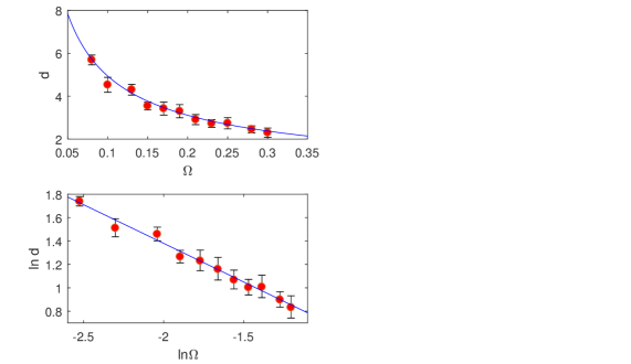
Figure 4: (Left):The sheet distance $d$ as a function of $\Omega$ on a $\Omega-d$ plot: $d=\frac{1}{0.95}\Omega^{-\frac{2}{3}}$. (Right):The sheet distance $d$ as a function of $\Omega$ on a Log-Log plot. The straight line is the best fit to $\ln d=a\ln\Omega+b$ with $a=-0.655\pm 0.027$ and $b=0.060\pm 0.048$.

According to the calculation by Landau and Lifshitz Landau , the distance d between sheets is determined by the surface tension $\sigma$ of the soliton and the kinetic energy of the counterflow $(v_{n}-v_{s})$ outside the sheet, where $v_{n}$ is the normal fluid velocity and $v_{s}$ is the vortex-free superfluid velocity. In unit volume, the counterflow energy is $\frac{1}{d}\int\frac{1}{2}\rho_{s}(v_{n}-v_{s})^{2}dy=\frac{\rho_{s}\Omega^{2}d^{2}}{6}$, and the surface energy is $\frac{\sigma}{d}$, where $\rho_{s}$ is the superfluid mass density. By the minimization of energy, one obtains

$$d=(\frac{3\sigma}{\rho_{s}\Omega^{2}})^{\frac{1}{3}}.$$ (13)

We confirm that the formula also hold in the two component holographic superfluid, a sample result when $\epsilon=0,\eta=0.2$ is plotted in In Fig.4.

As another important properties of superfluid, the Feynman linear relation between the excited vortex numbers and angular velocity in one component superfluid may can naturally generalizes to a two component superfluid as

$$N_{j}=\frac{M_{j}\Omega}{\pi\hbar}.$$ (14)

In the holographic model we also investigated the validity of the Feynman relation in the two-component system and found no obvious deviations from it, since the two components are of the same mass then $N_{1}=N_{2}$. A sample result is given in Fig. 5 for $\epsilon=0,\eta=0.2$.

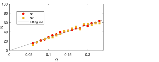
Figure 5: Vortex number of both components vs. angular velocity $\Omega$. The straight line is the best fit to $N=a\Omega+b$ with $a=286.62\pm 9.77$ and $b=-1.69\pm 1.39$. The temperature is fixed to be $T=0.82T_{c}^{0}$.

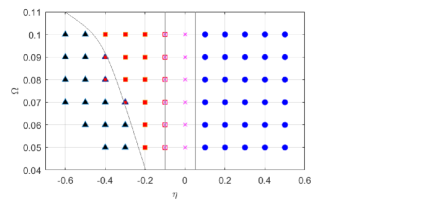
Figure 6: $\Omega-\eta$ phase diagram of the vortex states, where $\triangle$ symbolize triangular lattice, $\square$ symbolize square lattice, $\times$ stripe vortex and $\circ$ vortex sheet lattice.

Furthermore, the phase diagram of the vortex structures in the intercomponent direct coupling $\eta$ versus rotation-frequency $\Omega$ was investigated, see Fig.6. The upper limit of the rotation frequency is set by $\Omega=0.1$ while the bottom limit is set by $\Omega=0.05$. The diagram show a transition from triangular lattices to square lattices and then stripe and sheet. When $\eta>0.05$, where is the region of phase separation, it always presents a sheet solution, which confirms our conjecture that the sheet solution found in Fig.3 under rotation is a result of phase separation.

V Conclusions and discussions

The properties of a two component superfluid obtained from AdS/CFT correspondence in our simulation can be compared to experiments, for example, in ref Schweikhard , the interlaced square lattice similar to Fig.2(c) was observed. Also in the experiment, the vortex core size of the interlocked are bigger than the one of single component, which we can also observe in Fig. 2. The sheet solution is expected in the highly separated region, which may can be observed experimentally in a two component BECs with tunable intercomponent interactions, which can be deeply in a phase separate regionThalhammer ; Papp . The two species are of the same mass, then the vortex core size are the same as shown in Fig. 2 and Fig.3. Using of different masses for the two components, we will realize a coexistence system of vortices with different vortex-core sizes, then the lattice structure shown in this work may be changed, which deserves to be studied in future.

Finally we comment on the properties of the finite temperature holographic two-component superfluid that are different from that of the weakly coupled zero temperature two-component BECs studied in Ueda ; Kasamatsu . Firstly, in the finite temperature strongly coupled holographic superfluid, the increased correlation length will delay the appearance of the phase separation phase at a larger repulsive coupling $\eta$ (see Fig.1 (a)). Secondly, the triangle and square lattices (see Fig.2 (a-d)) are less perfect in the holographic model compared to the perfect lattices founded in a very low temperature rotating spinor BECsSchweikhard ; the distortions of regular lattices found here is very likely due to the relatively high temperature close to $T_{c}^{0}$, since we have confirmed that at higher temperature $T=0.98T_{c}^{0}$, the vortex lattice becomes more disorder with a lower translational symmetry, this is also the case we observed in a single component superfluid for different temperaturesXia:2019eje . This is probably due to the fact that the larger vortices at higher temperature are more closer then the interaction between vortices is large which prevents the lattices to organized as a perfect lattice. Employ a gravity dual theory at zero temperature defined in AdS solitonNishioka:2009zj , the vortex lattices with perfect hexagonal and square symmetry might be expected to be obtained in single and two-component superfluid respectively. Thirdly, even at finite temperature, the perfect sheet solutions with accurately equidistant layers were obtained for the first time from holography (see Fig.3) in the deeply phase separated regime, this is probably due to the strongly coupling nature of the holographic model. While in a weakly coupled zero temperature BECsKasamatsu , the distances $d$ between sheets are not perfect equal which is harder to calculate when comparing the numerical results to the Landau-Lifshitz formula.

Acknowledgements.— We thank Li Li and Muneto Nitta for valuable comments. This work is supported by the National Natural Science Foundation of China (under Grant No. 11675140, 11705005, 11875095).

W.C.Y. and C.Y.X. contributed equally to this work.

References

- (1) J. M. Maldacena, Adv. Theor. Math. Phys. 2, 231 (1998).
- (2) S. S. Gubser, I. R. Klebanov, and A. M. Polyakov, Phys. Lett. B 428, 105 (1998).
- (3) E. Witten, Adv. Theor. Math. Phys 2, 253 (1998).
- (4) J. Zaanen, Y. W. Sun, Y. Liu and K. Schalm, “Holographic Duality in Condensed Matter Physics,” Cambridge University Press, 2015.
- (5) M. Ammon and J. Erdmenger, “Gauge/gravity duality: Foundations and applications,” Cambridge University Press, 2015
- (6) H. Liu and J. Sonner, arXiv:1810.02367 [hep-th].
- (7) A. Adams, P. M. Chesler, and H. Liu, Science 341, 368 (2013).
- (8) J. Sonner, A. del Campo and W. H. Zurek, Nature Commun. 6, 7406 (2015)
- (9) M. J. Bhaseen, J. P. Gauntlett, B. D. Simons, J. Sonner, and T. Wiseman, Phys. Rev. Lett. 110, 015301 (2013).
- (10) P. M. Chesler, A. M. Garcia-Garcia and H. Liu, Phys. Rev. X 5, 021015 (2015).
- (11) S. S. Gubser, Phys. Rev. D 78, 065034 (2008).
- (12) S. A. Hartnoll, C. P. Herzog, and G. T. Horowitz, Phys. Rev. Lett. 101, 031601 (2008).
- (13) C. P. Herzog, P. K. Kovtun and D. T. Son, Phys. Rev. D 79, 066002 (2009).
- (14) Feynman R P “Application of quantum mechanics to liquid helium”, in Progress in Low Temperature Physics Vol. 1 (Ed. C J Gorter) (Amsterdam: North-Holland, 1955) p. 17.
- (15) C. Y. Xia, H. B. Zeng, H. Q. Zhang, Z. Y. Nie, Y. Tian and X. Li, arXiv:1904.10925 [hep-th].
- (16) X. Li, Y. Tian and H. Zhang, arXiv:1904.05497.
- (17) M. Montull, A. Pomarol and P. J. Silva, Phys. Rev. Lett. 103, 091601 (2009).
- (18) O. Domenech, M. Montull, A. Pomarol, A. Salvio and P. J. Silva, JHEP 1008, 033 (2010).
- (19) V. Keranen, E. Keski-Vakkuri, S. Nowling, and K. Yogendran, Phys.Rev. D 81, 126012 (2010).
- (20) K. Maeda, M. Natsuume and T. Okamura, Phys. Rev. D 81, 026002 (2010).
- (21) Oscar J. C. Dias, G. T. Horowitz, N. Iqbal and J. E. Santos, JHEP 1404, 096 (2014).
- (22) G. Tallarita, R. Auzzi, and A. Peterson, JHEP 1903, 114 (2019).
- (23) K. Kasamatsu, M. Tsubota, M. Ueda, Int. J. Mod. Phys. B 19, 1835 (2005)
- (24) Tin-Lun Ho and V. B. Shenoy, Phys. Rev. Lett. 77, 3276 (1996).
- (25) B. D. Esry, Chris H. Greene, James P. Burke, Jr., and John L. Bohn, Phys. Rev. Lett. 78, 3594 (1997)
- (26) E. Timmermans, Phys. Rev. Lett. 81, 5718(1998)
- (27) D. S. Hall, M. R. Matthews, C. E. Wieman, and E. A. Cornell, Phys. Rev. Lett. 81, 1539 (1998).
- (28) K. Kasamatsu, M. Tsubota, and M. Ueda, Phys. Rev. Lett. 91, 150406 (2003).
- (29) K. Kasamatsu and M. Tsubota, Phys. Rev. A 79, 023606 (2009).
- (30) L.D. Landau and E.M. Lifshitz, On the rotation of liquid helium, Doklady Akademii Nauk SSSR 100, 669-672 (1955).
- (31) Ü. Parts, E.V. Thuneberg, G.E. Volovik, J.H. Koivuniemi, V.M.H. Ruutu, M. Heinilä, J.M. Karimäki, and M. Krusius, Phys. Rev. Lett. 72, 3839 (1994).
- (32) G. E. Volovik, Usp. Fiz. Nauk 185, 970 (2015).
- (33) W. Y. Wen, M. S. Wu and S. Y. Wu, Phys. Rev. D 89, 066005 (2014)
- (34) P. N. Galteland, E. Babaev, and A. Sudbø, Phys. Rev. A 91, 013605 (2015).
- (35) M. Cipriani and M. Nitta, Phys. Rev. Lett. 111, 170401 (2013).
- (36) F. Bigazzi, A. L. Cotrone, D. Musso, N. Pinzani Fokeeva and D. Seminara, JHEP 1202, 078 (2012).
- (37) D. Musso, JHEP 06, 083 (2013).
- (38) D. S. Hall, M. R. Matthews, J. R. Ensher, C. E. Wieman, and E. A. Cornell, Phys. Rev. Lett. 81, 1539 (1998).
- (39) J. Stenger, S. Inouye, D. M. Stamper-Kurn, H. J. Miesner, A. P. Chikkatur, and W. Ketterle, Nature (London) 396, 345 (1998).
- (40) R. A. Janik, J. Jankowski and H. Soltanpanahi, Phys. Rev. Lett. 119, 261601 (2017).
- (41) M. Attems, Y. Bea, J. Casalderrey-Solana, D. Mateos and M. Zilhäo, arXiv:1905.12544 [hep-th].
- (42) M. S. Wu, S. Y. Wu and H. Q. Zhang, JHEP 1605, 011 (2016).
- (43) V. Schweikhard, I. Coddington, P. Engels, S. Tung, and E. A. Cornell, Phys. Rev. Lett. 93, 210403 (2004).
- (44) G. Thalhammer, G. Barontini, L. De Sarlo, J. Catani, F. Minardi, and M. Inguscio, Phys. Rev. Lett. 100, 210402 (2008).
- (45) S. B. Papp, J. M. Pino, and C. E. Wieman, Phys. Rev.Lett. 101, 040402 (2008).
- (46) T. Nishioka, S. Ryu and T. Takayanagi, JHEP 1003, 131 (2010).