Boltzmann distribution of sediment transport

Abstract

The coupling of sediment transport with the flow that drives it allows rivers to shape their own bed. Cross-stream fluxes of sediment play a crucial, yet poorly understood, role in this process. Here, we track particles in a laboratory flume to relate their statistical behavior to the self organization of the granular bed they make up. As they travel downstream, the transported grains wander randomly across the bed’s surface, thus inducing cross-stream diffusion. The balance of diffusion and gravity results in a peculiar Boltzmann distribution, in which the bed’s roughness plays the role of thermal fluctuations, while its surface forms the potential well that confines the sediment flux.

When water flows over a layer of solid grains, the shear stress it exerts on the sediment’s surface entrains some of the grains as bedload Bagnold (1973); Mouilleron et al. (2009). Eventually, the flow deposits the traveling grains downstream Charru et al. (2004); Lajeunesse et al. (2010). The balance of entrainment and deposition deforms the sediment bed Exner (1925), thus changing the flow and the distribution of shear stress. This coupling, through various instabilities, generates sand ripples in streams Coleman and Eling (2000); Charru and Hinch (2006), rhomboid patterns on beaches Devauchelle et al. (2010), alternate bars in rivers Colombini et al. (1987) and, possibly, meanders Ikeda et al. (1981); Johannesson and Parker (1989); Liverpool and Edwards (1995); Seminara (2006).

More fundamentally, the coupling of water flow and sediment transport is the mechanism by which alluvial rivers choose their own shape and size, as they build their bed out of the sediment they carry Henderson (1961); Parker et al. (2007); Devauchelle et al. (2011); Seizilles et al. (2013). To do so, however, rivers need to transport sediment not only downstream, but also across the flow Parker (1978a, b). On a slanted bed, of course, gravity will pull traveling grains downwards; it thus diverts the sediment flux away from the banks of a river Kovacs and Parker (1994); Chen et al. (2009). What mechanism opposes this flux to maintain the river’s bed remains an open question. Here, we suggest the inherent randomness of sediment transport plays a major role in the answer.

The velocity of bedload grains fluctuates as they travel over the rough bed, and the bedload layer constantly exchanges particles with the latter Roseberry et al. (2012), thus calling for a statistical description of bedload transport Jenkins and Hanes (1998); Furbish et al. (2012). At its simplest, this theory involves a population of non-interacting grains traveling, on average, at velocity $V_{x}$, close to the grain’s settling velocity Lajeunesse et al. (2010, 2017). If $n$ is the surface density of traveling grains, the downstream flux of sediment reads $q_{s}=nV_{x}$. As long as sediment transport is weak, the traveling grains do not interact significantly, and their average velocity $V_{x}$ can be treated as a constant. Both the streamwise and cross-stream velocities, nonetheless, fluctuate significantly Roseberry et al. (2012); Seizilles et al. (2014).

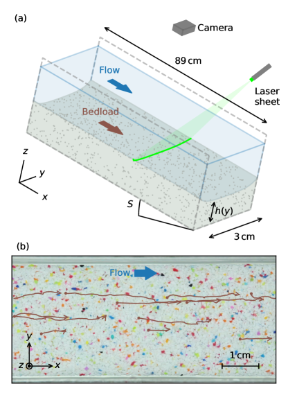
Figure 1: (a) Experimental setup and notations. Two Plexiglas panels confine the flume laterally. The $x$ axis is aligned with the flow. (b) Part of the camera’s field of view (background picture) with superimposed grains trajectories (red lines). Dots and arrows indicate beginning and end of trajectories, respectively. Data from experimental run #1.

Table 1: Experimental parameters. Run #1 serves as an example in all figures.

Run	Sediment input	Fluid input	Slope	Tracking time
#	[grains s-1]	[L min-1]	%	[min]
1	42.4	0.83	0.88	93
2	37.4	1.12	0.79	100
3	21.3	0.87	0.77	181
4	19.7	1.13	0.69	68
5	19.2	1.11	0.71	124

A little-investigated consequence of these fluctuations is the cross-stream dispersion they induce Nikora et al. (2002); Aussillous et al. (2016). Indeed, as it travels downstream, a grain bumps into immobile grains like a ball rolling down a Galton board. The random deviations so induced turn its trajectory into a random walk across the stream Samson et al. (1998); Seizilles et al. (2014). We thus expect a cross-stream, Fickian flux to bring traveling grains towards the less populated areas of the bed (lower $n$). Mathematically,

$$q_{d}=-\ell_{d}\frac{\partial q_{s}}{\partial y}$$ (1)

where $q_{d}$ is the fluctuation-induced Fickian flux, $y$ is the cross-stream coordinate, and $\ell_{d}$ is the diffusion length, which scales with the amplitude of the trajectory fluctuations. Tracking resin grains in a water flume, Seizilles et al. found $\ell_{d}\approx 0.03\,d_{s}$ ($d_{s}$ is the grain size) Seizilles et al. (2014). To our knowledge, neither the cross-stream flux of grains $q_{d}$, nor its consequences on the bed’s shape, have been directly observed.

To measure the Fickian flux $q_{d}$, we set up a particle-tracking experiment in a 3 cm-wide flume {Fig. 1(a), detailed experimental methods in Sup. Mat.}. We inject into the flume a mixture of water and glycerol (density $\rho=1160\,$g L^-1, viscosity $\eta=10\,$cP) at constant rate (Tab. 1). We use a viscous fluid to keep the flow laminar (Reynolds number below 250). Simultaneously, and also at constant rate, we inject sieved resin grains (median diameter $d_{s}=827\,\mu$m, density $\rho_{s}=1540\,$g L^-1). After a few hours, the sediment bed reaches its equilibrium shape.

This equilibrium, however, is a dynamical one: the flow constantly entrains new grains, and deposits other ones onto the bed. A camera mounted above the flume films the traveling grains through the fluid surface, at a frequency of 50 fps [Tab. 1, Fig. 1(b), Sup. Movie]. Although made of the same material, the grains are of different colors, which allows us to locate them individually on each frame. We then connect their locations on successive frames to reconstruct their trajectories with a precision of $0.1\,d_{s}$ (Munkres, 1957, Sup. Mat.).

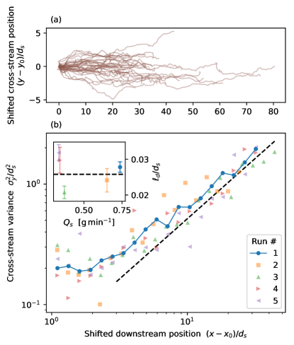
Figure 2: Cross-stream dispersion of the traveling grains. (a) 34 trajectories from run #1, with starting point shifted to origin. (b) Cross-stream variance of shifted trajectory. Dashed black line: linear relation with diffusion length $\ell_{d}$ fitted to data [Eq. (2)]. Inset: $\ell_{d}$ fitted independently to individual runs. Error bars show uncertainty.

The resulting trajectories are mostly oriented downstream, as expected, but they also fluctuate sideways, like in previous bedload experiments (Nikora et al., 2002; Roseberry et al., 2012; Seizilles et al., 2014). These fluctuations cause them to disperse across the stream as they travel downstream [Fig. 2(a)]. We now distribute all our trajectories into 25 logarithmically-spaced bins, according to their travel length $x-x_{0}$ ($x_{0}$ is the starting point of each trajectory), and calculate the variance $\sigma_{y}^{2}$ for each bin [Fig. 2(b)]. We find that, for trajectories longer than a few grain diameters, the cross-stream variance increases linearly with the travel distance. Seizilles et al. (2014) interpreted a similar relationship as the signature of a random walk across the stream (they also found that the auto-correlation of the cross-stream trajectories decays exponentially). Accordingly, we now fit the relation $\sigma_{y}^{2}=2\ell_{d}(x-x_{0})$ to our trajectories (beyond $3d_{s}$ downstream of their starting point). To estimate $\ell_{d}$, we treat the above relation as the reduced major axis of our data set: $2\ell_{d}=\mathrm{std}(\sigma_{y}^{2})/\mathrm{std}(x-x_{0})$, where the standard deviation is over bins, that is, over the data points of Fig. 2(b). Using our entire data set (typically $3\times 10^{4}$ trajectories per run), we get

$$\ell_{d}=\left(0.024\pm 0.002\right)d_{s}\,.$$ (2)

where the uncertainty is the expected standard deviation of $\ell_{d}$. This value is close to previous measurements in pure water Seizilles et al. (2014), although it is most likely affected by the physical properties of the fluid and of the grains.

That diffusion expresses itself through a length scale, as opposed to a diffusion coefficient, betrays its athermal origin: it is the driving (here, the flow) that sets the time scale. This property relates bedload diffusion to the diffusion induced by shearing in granular materials and foams Utter and Behringer (2004); Fenistein et al. (2004); Debregeas et al. (2001).

Although fluctuations disperse the traveling grains across the stream, most grains travel near the center of the channel [Fig. 1(b)]. According to Eq. 1, such a concentration should induce a Fickian flux towards the flume’s wall. At equilibrium, we expect gravity to counteract this flux; for this to happen, the bed’s cross section needs to be convex. In fact, the bed cannot maintain a flat surface: in this configuration, the fluid-induced shear stress would be weaker near the sidewalls, and so would the intensity of sediment transport. Bedload diffusion would then bring more grains towards the bank, thus preventing equilibrium. In the following, we investigate this coupling.

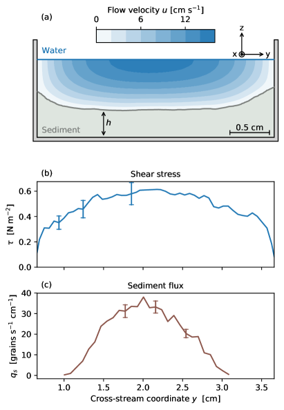
Figure 3: (a) Average cross-section of the flume during run #1. Beige: sediment layer. Blue colormap: downstream flow velocity calculated with finite elements. (b) Flow-induced shear stress on the bed. (c) Sediment flux measured by grain tracking. Error bars indicate measurement uncertainty (Sup. Mat.).

We use an inclined laser sheet to measure the elevation profile of the bed [Fig. 1(a), Sup. Mat]. The laser source is fixed on a rail which allows it to scan the flume over 20 cm. We evaluate the tilt of the rail by scanning a tub of still milk; it is less than $0.03\,$%. At the end of an experimental run, we switch off the fluid input; this brings the bed to a standstill in a matter of seconds. We then let the fluid drain out of the flume, and use the laser scanner (i) to measure the bed’s downstream slope $S$ (Tab. 1) and (ii) to spatially average the bed’s cross-section, $h(y)$ [Fig. 3(a)]. We find that the sediment bed is convex for all our experimental runs. Its surface gently curves upwards near the center of the flume, and steepens near the walls. This observation indicates that the sediment bed has spontaneously created a potential well to confine the traveling particles in its center.

Unfortunately, measuring the flow depth based on the deflection of the laser beam proved imprecise. Instead, we used finite elements to solve the Stokes equation in two dimensions (Hecht, 2012, Sup. Mat.), namely:

$$\eta\nabla^{2}u=\rho gS\,,$$ (3)

where $u$ is the streamwise velocity of the fluid. We further assume that the free surface is flat, that the viscous stress vanishes there ($\partial u/\partial z=0$, where $z$ is the vertical coordinate) and that the fluid does not slip at the bed’s surface ($u=0$). Knowing the bed’s downstream slope $S$, we then adjust the elevation of the water surface to match the fluid discharge. In addition to the flow depth, this computation provides us with the velocity field of the flow [Fig. 3(a)], and thus the intensity of the viscous stress $\tau$ that the fluid exerts on the bed [Fig. 3(b)]. We find that, like the sediment bed, the viscous stress varies across the flume; it reaches a maximum at the center of the channel, and vanishes where the bed’s surface joins the walls—as expected for a laminar flow.

We now wish to relate the flow-induced stress to sediment transport. To measure the latter, we divide the flume’s width into 50 bins, and count the trajectories that cross a constant-$x$ line within each bin, per unit time. This procedure yields a sediment-flux profile (Sup. Mat.). Repeating it for 10 different lines across the channel, we obtain an average sediment-flux profile, $q_{s}(y)$ [we keep only data points for which the relative uncertainty is less than one, Fig. 3(c)]. In accordance with the distribution of trajectories in Fig. 1(b), the sediment flux appears concentrated around the center of the flume. It vanishes quickly away from the center, much before the fluid-induced stress has significantly decreased.

Following Shields, we now relate the sediment flux to the ratio of the fluid-induced stress to the weight of a grain, $\theta$ Shields (1936):

$$\theta=\frac{\tau}{(\rho_{s}-\rho)gd_{s}}$$ (4)

where $g$ is the acceleration of gravity. The Shields parameter is an instance of the Coulomb friction factor; strictly speaking, on a convex bed like that of Fig. 3(a), its expression should include the cross-stream slope, $\partial h/\partial y$ Seizilles et al. (2013). In our experiments, however, we find that this correction is insignificant where sediment transport is measurable. Accordingly, we content ourselves with the approximate expression of Eq. (4).

Plotting the intensity of the sediment flux as a function of the force driving it, in the form of the Shields parameter $\theta$, shows a well-defined threshold [Fig. 4(a)]: no grain moves when the fluid-induced stress is too weak to overcome its weight, but the sediment flux increases steeply past this threshold. This emblematic behavior, apparent in a single experimental run, is confirmed by the superimposition of our five experimental runs [Fig. 4(a)]. Indeed, within the variability of the measurements, the five corresponding transport laws gather around a common relation, which we may treat as linear above the threshold Shields stress $\theta_{t}$ Seizilles et al. (2014):

$$q_{s}=q_{0}\,(\theta-\theta_{t})$$ (5)

where $q_{0}$ is a constant of order $(\rho-\rho_{s})g/\eta$. Fitting this transport law to our complete data set, we get $q_{0}=544\pm 48$ grains s^-1 cm^-1 and $\theta_{t}=0.167\pm 0.003$, where the uncertainty is the standard deviation over individual runs. These values correspond to a typical transport law in a laminar flow Mouilleron et al. (2009); Seizilles et al. (2014).

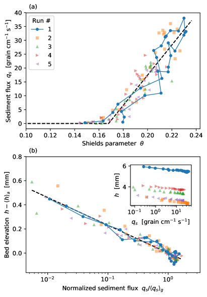
Figure 4: (a) Local sediment transport law. Marker types indicate individual experimental runs. Solid line: experimental run #1. Dashed black line: Equation (5) with $q_{0}=544$ grains s^-1 m^-1 and $\theta_{t}=0.17$. (b) Distribution of sediment flux with respect to bed elevation. Colors and markers similar to (a). Dashed black line: Bolztmann distribution [Equation (8)] with $\lambda_{B}=0.10$ mm.

The local intensity of the flow-induced stress controls the local flux of sediment—just as expected. More surprisingly, perhaps, the sediment bed needs to adjust its shape so that, in total, the flume conveys the sediment discharge that we impose at the inlet. We suggest that it does so by balancing the Fickian flux, $q_{d}$, which pushes the traveling grains away from the flume’s center, with the gravity-induced flux, $q_{g}$, which pulls them towards the lowest point of the bed’s surface. As a first approximation, we may assume that the latter is proportional (i) to the cross-stream slope of the bed and (ii) to the local intensity of the downstream flux of sediment, $q_{s}$. Mathematically,

$$q_{g}=-\alpha\,q_{s}\frac{\partial h}{\partial y}$$ (6)

where $\alpha$ is a dimensionless constant. Although conducted in air, the experiments of Chen et al. (2009) suggest that it should be of order unity or less.

At equilibrium, the gravity-induced flux $q_{g}$ needs to match the Fickian flux $q_{d}$. Adding Eqs. (6) and (1) yields the Boltzmann equation, which we readily integrate into an exponential distribution:

$$q_{s}(y)=q_{0}\,\exp\left[-\frac{h(y)}{\lambda_{B}}\right]\,,$$ (7)

where $q_{0}$ is an integration constant, and $\lambda_{B}=\ell_{d}/\alpha$ is the characteristic length of the distribution. Distinctively, this distribution relates two quantities ($q_{s}$ and $h$) that depend on the space coordinate $y$, but the latter does not explicitly appear in its expression. This, however, does not make it a local relationship: unlike the transport law of Eq. (5), it features an integration constant which depends on the sediment and water discharges of each experiment. These properties, typical of a Boltzmann distribution, appear when plotting the bed elevation as a function of the sediment discharge [Fig. 4(b), inset]. For each experiment, the data points trace twice the same line in the semi-logarithmic space, as they go from one side of the channel to the other, but the position of this line depends on the experimental run.

To bring all our experiments into the same space, we now divide Eq. (7) by its geometrical mean. This rids us of the integration constant $q_{0}$, and turns the distribution of sediment transport into

$$\frac{q_{s}(y)}{\langle q_{s}\rangle_{g}}=\exp\left[-\frac{h(y)-\langle h\rangle_{a}}{\lambda_{B}}\right]\,,$$ (8)

where $\langle\cdot\rangle_{g}$ and $\langle\cdot\rangle_{a}$ are the geometric and arithmetic means, respectively. Within the variability of our observations, the data points from all experimental runs gather around a straight line, which we interpret as Eq. (8). Fitting the characteristic length $\lambda_{B}$ to our entire data set, we find $\lambda_{B}=0.10\pm 0.01\,$mm, where the uncertainty is the standard deviation over individual runs. More tellingly, this value corresponds to

$$\lambda_{B}=(0.12\pm 0.02)\,d_{s}\,,$$ (9)

showing that the characteristic length compares with the grain size. Returning to the definition of $\lambda_{B}$, we find that the constant $\alpha$ in Eq. (6) is about $0.2$, in agreement with previous estimates Chen et al. (2009).

Although temperature plays no part here, the structure of Eq. (8), as well as its derivation, makes it a direct analog of the Boltzmann distribution, where the cross-stream deviations of the grains’ trajectories play the role of thermal fluctuations. Pursuing this analogy, we suggest that the scale of $\lambda_{B}$ is inherited from the roughness of the underlying granular bed, which we believe causes the cross-stream deviations—a mechanism reminiscent of, but somewhat simpler than, the shear-induced diffusion observed in granular flows Utter and Behringer (2004); Fenistein et al. (2004); Debregeas et al. (2001). To support this hypothesis, however, we would need more experiments with different grains and fluids.

The familiarity of the Boltzmann distribution should not obscure the peculiarity of the phenomenon we report here. We naturally expect that random walkers will distribute themselves in a potential well according to this distribution; what is remarkable here, however, is that the system spontaneously chooses the shape of the potential well to match the transport law. This is possible only because the sediment bed is made of the very particles that roam over its surface.

A practical consequence of this self-organization is that sediment transport cannot be uniform across a flume, thus prompting us to reevaluate the transport laws measured in this classical set-up. (If we were to assume uniformity in our experiments, we would underestimate $q_{0}$ by a factor of two.) In the context of dry granular flows, the traditional rotating-drum experiment has been challenged on similar grounds Jop et al. (2005).

Much remains to be done to understand how the bed builds its own shape. To do so, we will have to drop the equilibrium assumption. A first step in that direction was to demonstrate theoretically that the cross-stream diffusion of sediment could generate a distinctive instability, but the associated pattern has not been observed yet Abramian et al. (2018). More generally, the consequences of bedload diffusion on the morphology of rivers, and ultimately on that of the landscapes they carve, belong to uncharted territory.