CT Data of a Pen-Spring: Application to Under-Sampled Dynamic X-ray Tomography

Abstract

This is the documentation of Computed Tomography (CT) data of a pen-spring. The open data set is available here and can be freely used for scientific purposes with appropriate references to the data and to this document in http://arxiv.org/. The provided data set includes the X-ray sinograms (finalSino) of a single 2D slice from a different height of the spring. The finalSino was obtained from a measured 10-projection or 100-projection sinogram using fan-beam geometry by down-sampling and taking logarithms. The data set includes also those original measured sinograms and corresponding measurement matrices.

1 Introduction

In this documentation, Computed Tomography (CT) data of a pen-spring was acquired. The goal of this data set is to test dynamic x-ray algorithm using under-sampled data. The data is prepared for dynamic case, where the under-sampled data sets are challenging, but also interesting [1, 2, 3, 4]. In practice, there are also applications in cardiac CT [5, 6]. Twenty five millimeters long pen-spring with $4$ mm diameter, made from $0,5$ mm thick thread was stretched a little to make the shape less frequent. The object was lifted $0.25$ mm between the measurements to get the full circle from the mid slices of the spring. With 10 projection the spring was measured with 33 different height to get data from three consecutive circles. With 100 projection the spring was measured with 11 different height so that the data included one full circle of spring. See Figure 1. All those 11 different 2D slices are shown in Figure 8. In addition, periodic data sets could be produced by stacking the corresponding sinogram and the measurement matrix accordingly.

Figure 1: The blue arrow shows where 11 measurements with 100 projections were taken and the red arrow shows where the 33 measurements were taken with 10 projections.

2 Contents of the
data set

The data set contains the following data folders/files:
Data_64x10,
Data_64x25,
Data_256x25,
Data_64x100,
Data_256x100,
FilteredBackProjection100.png,
Reconstruction.mp4

First five data folders include CT sinograms. Folders contain also the corresponding measurement matrices either with the resolution $64\times 64$ or $256\times 256$ as spatial resolution and $33$ or $11$ as a temporal resolution in 3D. Those 33 or 11 times instances are obtained by lifting the object little by little at a time between the measurements. The projection angles were same in every time step. Details of these data folders is shown in the Table 1. FilteredBackProjection100.png file is the filtered back projection image shown in Figure 9 and Reconstruction.mp4 file is the video made from reconstructions.

Folder	Size of Matrix A	Size of sinogram	Size of finalSino	Spatial resolution	Temporal resolution
Data_64x10	970 x 4096	1240 x 10	97 x 10	64	33
Data_64x25	2425 x 4096	1240 x 25	97 x 25	64	11
Data_256x25	9225 x 65536	1240 x 25	369 x 25	256	11
Data_64x100	9700 x 4096	1240 x 100	97 x 100	64	11
Data_256x100	36900 x 65536	1240 x 100	369 x 100	256	11

Table 1: Summary of the data folders.

Each folder contains the following variables:

1. Matrix A, the measurement matrix.

2. N measurement.mat files that contain the following variables for each N measurements (N equals temporal resolution):

   1. Matrix sinogram, the original measured sinogram.

   2. Matrix finalSino, the sinogram obtained from sinogram.

More details on the X-ray measurements are described in the Section 3 below. The model for the CT problem is

$${\tt A*x=finalSino(:)},$$ (1)

where finalSino(:) denotes the standard vector form of matrix finalSino in MATLAB and x is the reconstruction in vector form. In the reconstruction step, the main task is to find that vector x that executes the Equation (1) and possibly meets also some additional regularization requirements.

3 X-ray measurements

The data in the sinograms are X-ray tomographic (CT) data of a 2D cross-section of the pen-spring measured with Procon X-ray CTportable device shown in Figure 2.

• The X-ray source has 50 kV voltage and 50 W maximum ouput. The source is shown closely in Figure 4.

• The detector has 1 MP pixels and the pixelsize is 48 $\mu$m. The image files generated by the camera were $1024\times 967$ pixels in size. The detector is shown in Figure 5.

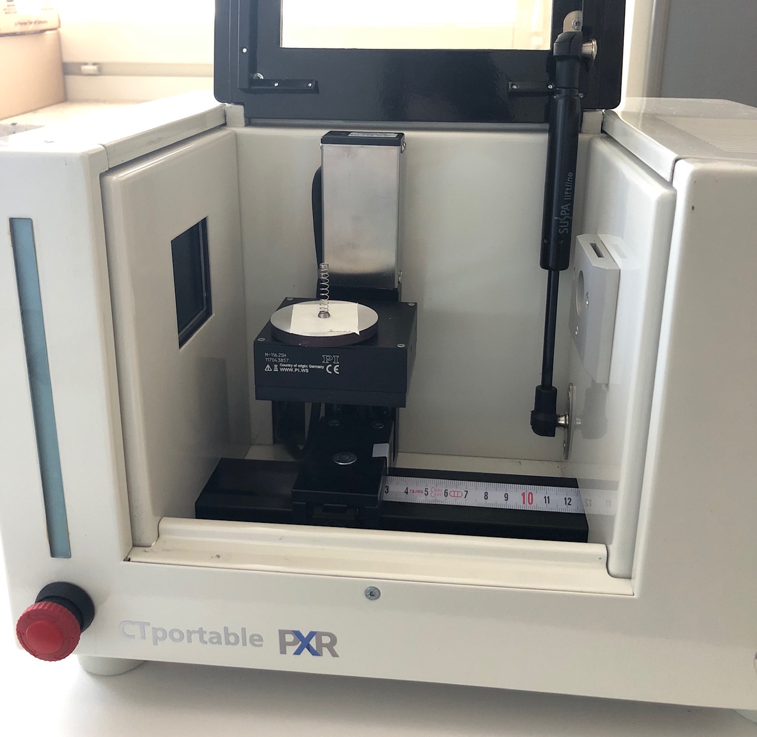
Figure 2: The Procon X-ray CTportable measurement device at Aalto University.

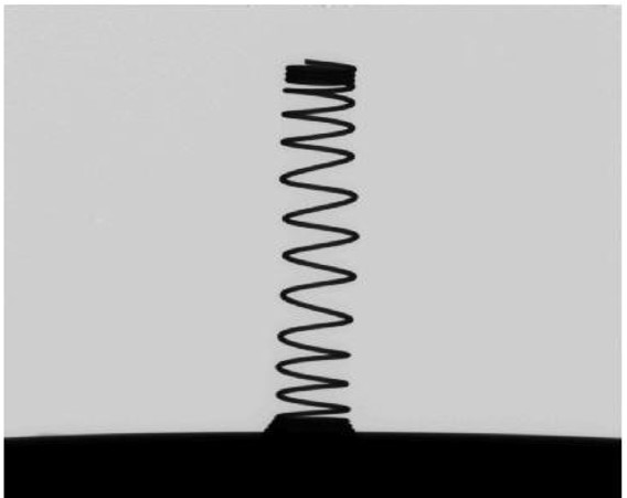
Figure 3: Resulting projection image of the spring.

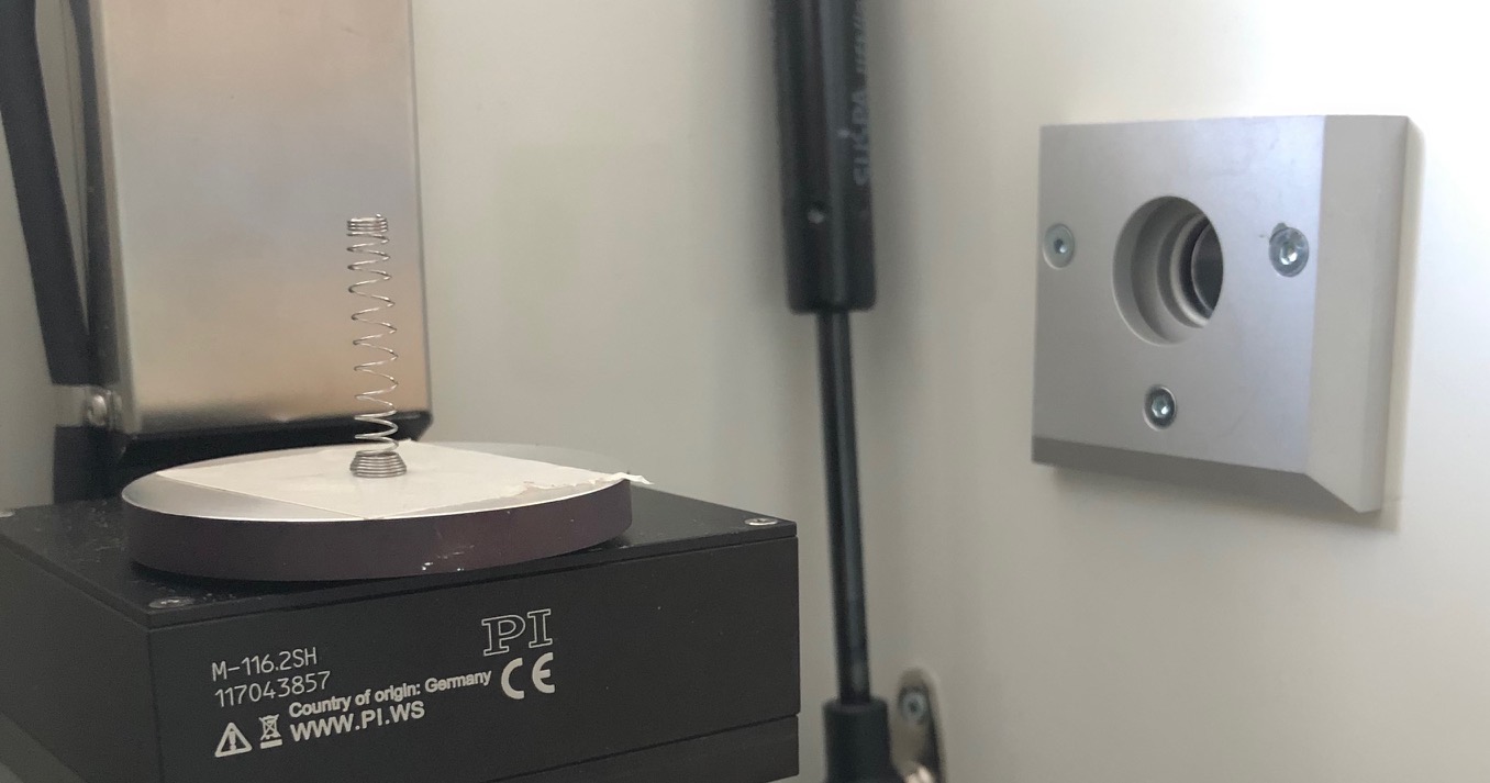
Figure 4: The Procon X-ray CTportable measurement device source.

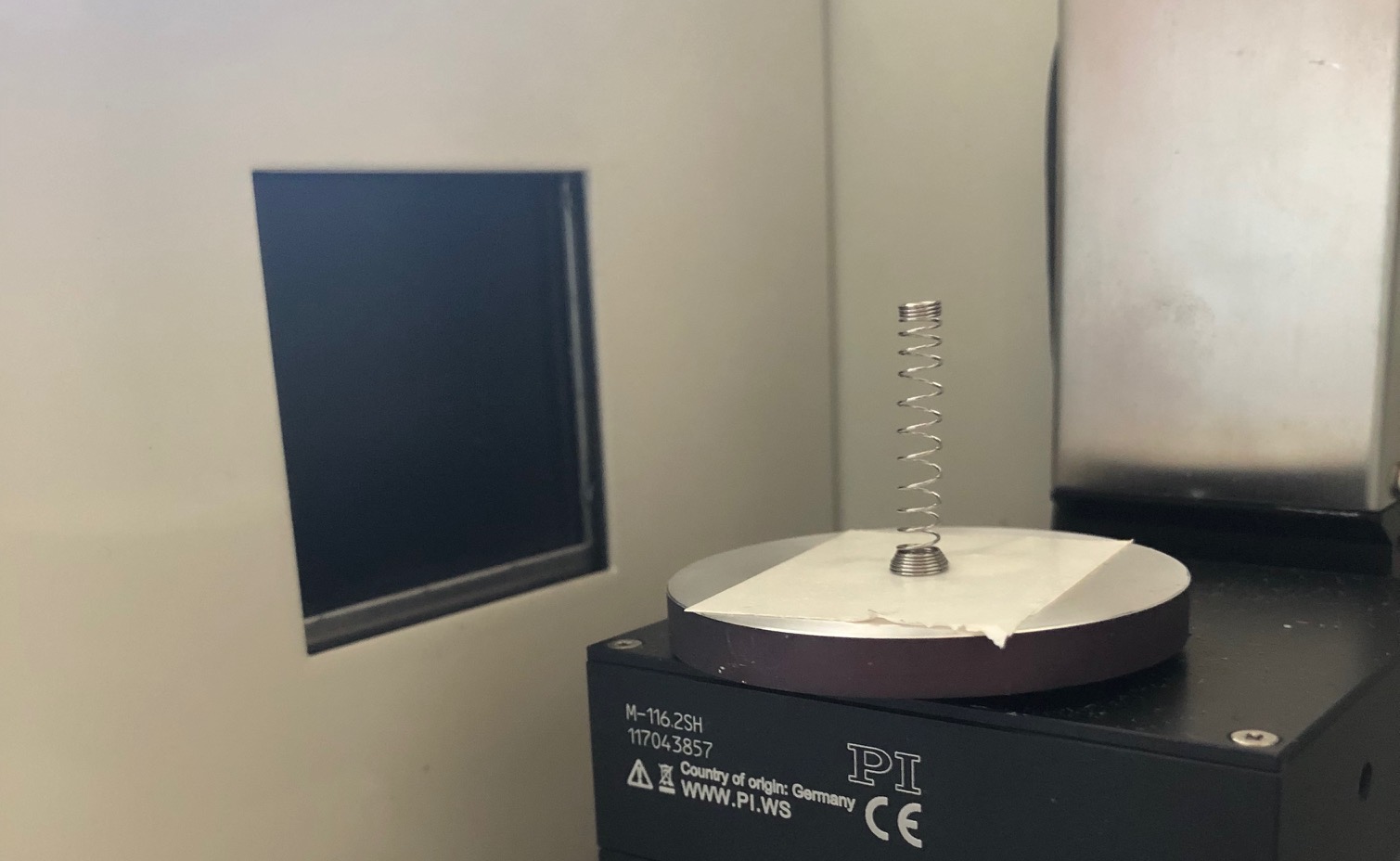
Figure 5: The Procon X-ray CTportable measurement device detector.

The measurement geometry is shown in Figure 6. A set of 360 fan-beam projections with resolution $1024\times 967$ was measured. The exposure time was 400 ms, X-ray tube acceleration voltage 50 kV and tube current 400 mA. See Figure 3 for an example of the resulting projection images.

From the 2D projection images, the middle rows (row 483) corresponding to the central horizontal cross-section of the spring target were taken to form a fan-beam sinogram of resolution $1024\times 10$ or $100$. These sinograms were further down-sampled by binning, taken logarithms and normalized to obtain the finalSino in all the files specified in Section 2. The organization of the pixels in the sinograms and the reconstructions is illustrated in Figure 7.

Figure 6: Geometry of the measurement setup. Here FOD and FDD denote the focus-to-object distance and the focus-to-detector distance, respectively; the black dot object is the center-of-rotation. The width of the detector (the blue line) is denoted by W. The orange dot is the X-ray source. To increase clarity, the $x$-axis and $y$-axis in this image are not in scale.

Figure 7: The organization of the pixels in the sinograms m = $[m_{1},m_{2},\ldots,m_{60K}]^{T}$ and reconstructions x = $[x_{1},x_{2},\ldots,x_{N^{2}}]^{T}$with $N=64$ or $N=256$ . The picture shows the organization for the first projection; after that in the full angular view case, the target takes steps ($3.6$ degree step for 10 projection data and $36$ degree step for 100 projection data) counter-clockwise (or equivalently the source and detector take steps clockwise) and the following columns of m are determined in an analogous manner.

Figure 8: 2D slice reconstructions from 11 different height of the spring, with 100 projections (from Data_256x100).

Figure 9: The filtered back-projection reconstruction (FilteredBackProjection100.png) of the spring, with 100 projections.

4 3D reconstruction

The video of the reconstruction of the target is available in the data set in Zenodo.

References

- [1] J. Hakkarainen, Z. Purisha, A. Solonen, and S. Siltanen, “Undersampled dynamic x-ray tomography with dimension reduction kalman filter,” IEEE Transactions on Computational Imaging, 2019.
- [2] T. A. Bubba, M. März, Z. Purisha, M. Lassas, and S. Siltanen, “Shearlet-based regularization in sparse dynamic tomography,” in Wavelets and Sparsity XVII, vol. 10394, p. 103940Y, International Society for Optics and Photonics, 2017.
- [3] G.-H. Chen, J. Tang, and S. Leng, “Prior image constrained compressed sensing (piccs): a method to accurately reconstruct dynamic ct images from highly undersampled projection data sets,” Medical physics, vol. 35, no. 2, pp. 660–663, 2008.
- [4] E. Niemi, M. Lassas, A. Kallonen, L. Harhanen, K. Hämäläinen, and S. Siltanen, “Dynamic multi-source x-ray tomography using a spacetime level set method,” Journal of Computational Physics, vol. 291, pp. 218–237, 2015.
- [5] Y. Hu, M. Jung, A. Oukili, G. Yang, J.-C. Nunes, J. Fehrenbach, G. Peyré, M. Bedossa, L. Luo, C. Toumoulin, et al., “Sparse reconstruction from a limited projection number of the coronary artery tree in x-ray rotational imaging,” in 2012 9th IEEE International Symposium on Biomedical Imaging (ISBI), pp. 804–807, IEEE, 2012.
- [6] C. Naoum, P. Blanke, and J. Leipsic, “Iterative reconstruction in cardiac ct,” Journal of cardiovascular computed tomography, vol. 9, no. 4, pp. 255–263, 2015.