Encoding high-cardinality
string categorical variables

Abstract

Statistical models usually require vector representations of categorical variables, using for instance one-hot encoding. This strategy breaks down when the number of categories grows, as it creates high-dimensional feature vectors. Additionally, for string entries, one-hot encoding does not capture morphological information in their representation.

Here, we seek low-dimensional encoding of high-cardinality string categorical variables. Ideally, these should be: scalable to many categories; interpretable to end users; and facilitate statistical analysis. We introduce two encoding approaches for string categories: a Gamma-Poisson matrix factorization on substring counts, and a min-hash encoder, for fast approximation of string similarities. We show that min-hash turns set inclusions into inequality relations that are easier to learn. Both approaches are scalable and streamable. Experiments on real and simulated data show that these methods improve supervised learning with high-cardinality categorical variables. We recommend the following: if scalability is central, the min-hash encoder is the best option as it does not require any data fit; if interpretability is important, the Gamma-Poisson factorization is the best alternative, as it can be interpreted as one-hot encoding on inferred categories with informative feature names. Both models enable autoML on string entries as they remove the need for feature engineering or data cleaning.

1 Introduction

Tabular datasets often contain columns with string entries. However, fitting statistical models on such data generally requires a numerical representation of all entries, which calls for building an encoding, or vector representation of the entries. Considering string entries as nominal—unordered—categories gives well-framed statistical analysis. In such situations, categories are assumed to be mutually exclusive and unrelated, with a fixed known set of possible values. Yet, in many real-world datasets, string columns are not standardized in a small number of categories. This poses challenges for statistical analysis. First, the set of all possible categories may be huge and not known a priori, as the number of different strings in the column can indefinitely increase with the number of samples. Second, categories may be related: they often carry some morphological or semantic links.

The classic approach to encode categorical variables for statistical analysis is one-hot encoding. It creates vectors that agree with the general intuition of nominal categories: orthogonal and equidistant [1]. However, for high-cardinality categories, one-hot encoding leads to feature vectors of high dimensionality. This is especially problematic in big data settings, which can lead to a very large number of categories, posing computational and statistical problems.

Data engineering practices typically tackle these issues with data-cleaning techniques [2, 3]. In particular, deduplication tries to merge different variants of the same entity [4, 5, 6]. A related concept is that of normalization, used in databases and text processing to put entries in canonical forms. However, data cleaning or normalization often requires human intervention, and are major costs in data analysis. To avoid the cleaning step, Similarity encoding [7] relaxes one-hot encoding by using string similarities [8]. Hence, it addresses the problem of related categories and has been shown to improve statistical analysis upon one-hot encoding [7]. Yet, it does not tackle the problem of high cardinality, and the data analyst much resort to heuristics such as choosing a subset of the training categories [7].

Here, we seek encoding approaches for statistical analysis on string categorical entries that are suited to a very large number of categories without any human intervention: avoiding data cleaning, feature engineering, or neural architecture search. Our goals are: i) to provide feature vectors of limited dimensionality without any cleaning or feature engineering step, even for very large datasets; ii) to improve statistical analysis tasks such as supervised learning; and iii) to preserve the intuitions behind categories: entries can be arranged in natural groups that can be easily interpreted. We study two novel encoding methods that both address scalability and statistical performance: a min-hash encoder, based on locality-sensitive hashing (LSH) [9], and a low-rank model of co-occurrences in character n-grams: a Gamma-Poisson matrix factorization, suited to counting statistics. Both models scale linearly with the number of samples and are suitable for statistical analysis in streaming settings. Moreover, we show that the Gamma-Poisson factorization model enables interpretability with a sparse encoding that expresses the entries of the data as linear combinations of a small number of latent categories, built from their substring information. This interpretability is very important: opaque and black-box machine learning models have limited adoption in real-world data-science applications. Often, practitioners resort to manual data cleaning to regain interpretability of the models. Finally, we demonstrate on 17 real-life datasets that our encoding methods improve supervised learning on non curated data without the need for dataset-specific choices. As such, these encodings provide a scalable and automated replacement to data cleaning or feature engineering, and restore the benefits of a low-dimensional categorical encoding, as one-hot encoding.

The paper is organized as follows. Section 2 states the problem and the prior art on creating feature vectors from categorical variables. Section 3 details our two encoding approaches. In section 4, we present our experimental study with an emphasis on interpretation and on statistical learning for 17 datasets with non-curated entries and 7 curated ones. Section 5 discusses these results, after which appendices provide information on the datasets and the experiments to facilitate the reproduction of our findings.

2 Problem setting and prior art

The statistics literature often considers datasets that contain only categorical variables with a low cardinality, as datasets in the UCI repository [10]. In such settings, the popular one-hot encoding is a suitable solution for supervised learning [1]: it models categories as mutually exclusive and, as categories are known a priory, new categories are not expected to appear in the test set. With enough data, supervised learning can then be used to link each category to a target variable.

2.1 High-cardinality categorical variables

However, in many real-world problems, the number of different string entries in a column is very large, often growing with the number of observations (Figure 1). Consider for instance the Drug Directory dataset. One of the variables is a categorical column with non proprietary names of drugs. As entries in this column have not been normalized, many different entries are likely related: they share a common ingredient such as alcohol (see I(a)). Another example is the Employee Salaries dataset. Here, a relevant variable is the position title of employees. As shown in I(b), here there is also overlap in the different occupations.

High-cardinality categorical variables may arise from variability in their string representations, such as abbreviations, special characters, or typos. Such non-normalized data often contains very rare categories. Yet, these categories tend to have common morphological information. Indeed, the number of unique entries grows less fast with the size of the data than the number of words in natural language (Figure 1). In both examples above, drug names and position titles of employees, there is an implicit taxonomy. Crafting feature-engineering or data-cleaning rules can recover a small number of relevant categories. However, it is time consuming and often needs domain expertise.

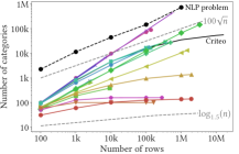
Figure 1: Number of categories versus number of samples. In general, a higher number of samples implies a higher number of categories for the respective variable. In general, the cardinality of categories grows slower than words in a typical NLP problem (Wikipedia articles in this case).

Notation

We write sets of elements with capital curly fonts, as $\mathcal{X}$. Elements of a vector space (we consider row vectors) are written in bold $\mathbf{x}$ with the $i$-th entry denoted by $x_{i}$, and matrices are in capital and bold $\mathbf{X}$, with $x_{ij}$ the entry on the $i$-th row and $j$-th column.

TABLE I: Examples of high-cardinality categorical variables.

Count	Non Proprietary Name
1736	alcohol
1089	ethyl alcohol
556	isopropyl alcohol
16	polyvinyl alcohol
12	isopropyl alcohol swab
12	62% ethyl alcohol
6	alcohol 68%
6	alcohol denat
5	dehydrated alcohol

(a) Count for some of the categories containing the word alcohol in the Drug Directory dataset. The dataset contains more than 120k samples.

Employee Position Title
Police Aide
Master Police Officer
Mechanic Technician II
Police Officer III
Senior Architect
Senior Engineer Technician
Social Worker III
Bus Operator

(b) Some categories in the Employee Salaries dataset. For 10 000 employees, there are almost 400 different occupations. Yet, they share relevant substrings.

Let $C$ be a categorical variable such that $\text{dom}(C)\subseteq\mathcal{S}$, the set of finite length strings. We call categories the elements of $\text{dom}(C)$. Let $s_{i}{\in}\mathcal{S},i{=}1...n$, be the category corresponding to the $i$-th sample of a dataset. For statistical learning, we want to find an encoding function $\text{enc:}\,\mathcal{S}\rightarrow\mathbb{R}^{d}$, such as $\text{enc}(s_{i})=\mathbf{x}_{i}$. We call $\mathbf{x}_{i}$ the feature map of $s_{i}$. Table II contains a summary of the main variables used in the next sections.

2.2 One-hot encoding, limitations and extensions

2.2.1 Shortcomings of one-hot encoding

From a statistical-analysis standpoint, the multiplication of entries with related information is challenging for two reasons. First, it dilutes the information: learning on rare categories is hard. Second, with one-hot encoding, representing these as separate categories creates high-dimension feature vectors. This high dimensionality entails large computational and memory costs; it increases the complexity of the associated learning problem, resulting in a poor statistical estimation [13]. Dimensionality reduction of the one-hot encoded matrix can help with this issue, but at the risk of loosing information.

Encoding all unique entries with orthogonal vectors discards the overlap information visible in the string representations. Also, one-hot encoding cannot assign a feature vector to new categories that may appear in the testing set, even if its representation is close to one in the training set. Heuristics such as assigning the zero vector to new categories, create collisions if more than one new category appears. As a result, one-hot encoding is ill suited to online learning settings: if new categories arrive, the entire encoding of the dataset has to be recomputed and the dimensionality of the feature vector becomes unbounded.

TABLE II: Summary of notations

Symbol	Definition
$\mathcal{S}$	Set of all finite-length strings.
$\mathcal{G}(s)\subseteq\mathcal{S}$	Set of all consecutive n-grams in $s\in\mathcal{S}$.
$\mathcal{V}=\bigcup_{i=1}^{n}\mathcal{G}(s_{i})$	Vocabulary of n-grams in the train set.
$C$	Categorical variable.
$n$	Number of samples.
$d$	Dimension of the categorical encoder.
$m=|\mathcal{V}|$	Cardinality of the vocabulary.
$\mathbf{F}\in\mathbb{R}^{n\times m}$	Count matrix of n-grams.
$\mathbf{X}\in\mathbb{R}^{n\times d}$	Feature matrix of $C$.
$\text{sim}:\mathcal{S}\times\mathcal{S}\rightarrow[0,1]$	String similarity.
$h_{k}:\mathcal{S}\rightarrow[0,1]$	Hash function with salt value equal to $k$.
$Z_{k}:\mathcal{S}\rightarrow[0,1]$	Min-hash function with salt value equal to $k$.

2.2.2 Similarity encoding for string categorical variables

For categorical variables represented by strings, similarity encoding extends one-hot encoding by taking into account a measure of string similarity between pairs of categories [7].

Let $s_{i}{\in}\mathcal{S},i{=}1...n$, the category corresponding to the $i$-th sample of a given training dataset. Given a string similarity $\text{sim}(s_{i},s_{j}){:}\,\mathcal{S}{\times}\mathcal{S}{\rightarrow}[0,1]$, similarity encoding builds a feature map $\mathbf{x}_{i}^{\text{sim}}{\in}\mathbb{R}^{k}$ as:

$$\mathbf{x}_{i}^{\text{sim}}\overset{\text{def}}{=}[\text{sim}(s_{i},s^{(1)}),\text{sim}(s_{i},s^{(2)}),\dots,\text{sim}(s_{i},s^{(k)})]\in\mathbb{R}^{k},$$ (1)

where $\{s^{(l)},l{=}1\dots k\}\subseteq\mathcal{S}$ is the set of all unique categories in the train set—or a subset of prototype categories chosen heuristically. With the previous definition, one-hot encoding corresponds to taking the discrete string similarity:

$$\text{sim}_{\text{one-hot}}(s_{i},s_{j})=\mathbbm{1}[s_{i}=s_{j}],$$ (2)

where $\mathbbm{1}[\cdot]$ is the indicator function.

Empirical work on databases with categorical columns containing non-normalized entries showed that similarity encoding with a continuous string similarity brings significant benefits upon one-hot encoding [7]. Indeed, it relates rare categories to similar, more frequent ones. In columns with typos or morphological variants of the same information, a simple string similarity is often enough to capture additional information. Similarity encoding outperforms a bag-of-n-grams representation of the input string, as well as methods that encode high-cardinality categorical variables without capturing information in the strings representations [7], such as target encoding [14] or hash encoding [15].

A variety of string similarities can be considered for similarity encoding, but [7] found that a good performer was a similarity based on n-grams of consecutive characters. This n-gram similarity is based on splitting the two strings to compare in their character n-grams and calculating the Jaccard coefficient between these two sets [16]:

$$\text{sim}_{\text{n-gram}}(s_{i},s_{j})=J(\mathcal{G}(s_{i}),\mathcal{G}(s_{j}))=\frac{|\mathcal{G}(s_{i})\cap\mathcal{G}(s_{j})|}{|\mathcal{G}(s_{i})\cup\mathcal{G}(s_{j})|}$$ (3)

where $\mathcal{G}(s)$ is the set of consecutive character n-grams for the string $s$. Beyond the use of string similarity, an important aspect of similarity encoding is that it is a prototype method, using as prototypes a subset of the categories in the train set.

2.3 Related solutions for encoding string categories

2.3.1 Bag of n-grams

A simple way to capture morphology in a string is to characterize it by the count of its character or word n-grams. This is sometimes called a bag-of-n-grams characterization of strings. Such representation has been shown to be efficient for spelling correction [16] or for named-entity recognition [17]. Other vectorial representations, such as those created by neural networks, can also capture string similarities [18].

For high-cardinality categorical variables, the number of different n-grams tends to increase with the number of samples. Yet, this number increases slower than in a typical NLP problem (see Figure 2). Indeed, categorical variables have less entropy than free text: they are usually repeated, often have subwords in common, and refer to a particular, more restrictive subject.

Representing strings by character-level n-grams is related to vectorizing text by their tokens or words. Common practice uses term-frequency inverse-document-frequency (tf-idf) reweighting: dividing a token’s count in a sample by its count in the whole document. Dimensionality reduction by a singular value decomposition (SVD) on this matrix leads to a simple topic extraction, latent semantic analysis (LSA) [19]. A related but more scalable solution for dimensionality reduction are random projections, which give low-dimensional approximation of Euclidean distances [20, 21].

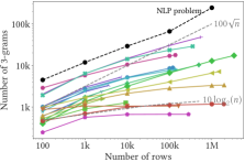
Figure 2: Number of 3-gram versus number of samples (colors as in Figure 1). The number of different n-grams tends to increase slower than in a typical NLP problem (Wikipedia articles in this case).

2.3.2 Word embeddings

If the string entries are common words, an approach to represent them as vectors is to leverage word embeddings developed in natural language processing [22, 23]. Euclidean similarity of these vectors captures related semantic meaning in words. Multiple words can be represented as a weighted sum of their vectors, or with more complex approaches [24]. To cater for out-of-vocabulary strings, FastText [25] considers subword information of words, i.e., character-level n-grams. Hence, it can encode strings even in the presence of typos. Similarly, Bert [26] uses also a composition of substrings to recover the encoding vector of a sentence. In both cases, word vectors computed on very large corpora are available for download. These have captured fine semantic links between words. However, to analyze a given database, the danger of such approach is that the semantic of categories may differ from that in the pretrained model. These encodings do not adapt to the information specific in the data at hand. Moreover, they cannot be trained directly on the categorical variables for two reasons: categories are typically short strings that do not embed enough context; and the number of samples in some datasets is not enough to properly train these models.

3 Scalable encoding of string categories

We now describe two novel approaches for categorical encoding of string variables. Both are based on the character-level structure of categories. The first approach, that we call min-hash encoding, is inspired by the document indexation literature, and in particular the idea of locality-sensitive hashing (LSH) [9]. LSH gives a fast and stateless way to approximate the Jaccard coefficient between two strings [27]. The second approach is the Gamma-Poisson factorization [28], a matrix factorization technique—originally used in the probabilistic topic modeling literature—that assumes a Poisson distribution on the n-gram counts of categories, with a Gamma prior on the activations. An online algorithm of the matrix factorization allows to scale the method with a linear complexity on the number of samples. Both approaches capture the morphological similarity of categories in a reduced dimensionality.

3.1 Min-hash encoding

3.1.1 Background: min-hash

Locality-sensitive hashing (LSH) [9] has been extensively used for approximate nearest neighbor search for learning [29, 30] or as an efficient way of finding similar objects (documents, pictures, etc.) [31] in high-dimensional settings. One of the most famous functions in the LSH family is the min-hash function [27, 32], originally designed to retrieve similar documents in terms of the Jaccard coefficient of the word counts of documents (see [33], chapter 3, for a primer). While min-hash is a classic tool for its collisions properties, as with nearest neighbors, we study it here as encoder for general machine-learning models.

Let $\mathcal{X}^{\star}$ be a totally ordered set and $\pi$ a random permutation of its order. For any non-empty $\mathcal{X}\subseteq\mathcal{X}^{\star}$ with finite cardinality, the min-hash function $Z(\mathcal{X})$ can be defined as:

$$Z(\mathcal{X})\overset{\text{def}}{=}\min_{x\in\mathcal{X}}\pi(x)$$ (4)

Note that $Z(\mathcal{X})$ can be also seen as a random variable. As shown in [27], for any $\mathcal{X},\mathcal{Y}{\subseteq}\mathcal{X}^{\star}$, the min-hash function has the following property:

$$\mathbb{P}\left(Z(\mathcal{X}){=}Z(\mathcal{Y})\right)=\frac{|\mathcal{X}\cap\mathcal{Y}|}{|\mathcal{X}\cup\mathcal{Y}|}=J(\mathcal{X},\mathcal{Y})$$ (5)

Where $J$ is the Jaccard coefficient between the two sets. For a controlled approximation, several random permutations can be taken, which defines a min-hash signature. For $d$ permutations $\pi_{j}$ drawn i.i.d., Equation 5 leads to:

$$\sum_{j=1}^{d}\mathbbm{1}[Z_{j}(\mathcal{X})=Z_{j}(\mathcal{Y})]\sim\mathcal{B}(d,J(\mathcal{X},\mathcal{Y})).$$ (6)

where $\mathcal{B}$ denotes the Binomial distribution. Dividing the above quantity by $d$ thus gives a consistent estimate of the Jaccard coefficient $J(\mathcal{X},\mathcal{Y})$.

Without loss of generality, we can consider the case of $\mathcal{X}^{\star}$ being equal to the real interval $[0,1]$, so now for any $x\in[0,1]$, $\pi_{j}(x)\sim\mathcal{U}(0,1)$.

Proposition 3.1.

Marginal distribution. If $\pi(x)\sim\mathcal{U}(0,1)$, and $\mathcal{X}{\subset}[0,1]$ such that $|\mathcal{X}|{=}k$, then $Z(\mathcal{X})\sim\text{Dir}(k,1)$.

Proof.

It comes directly from considering that:
$\mathbb{P}(Z(\mathcal{X}){\leq}z)=$ $1-\mathbb{P}(Z(\mathcal{X}){>}z)=1-\prod_{i=1}^{k}\mathbb{P}(\pi(x_{i})>z)=1-(1-z)^{k}$. ∎

Now that we know the distribution of the min-hash random variable, we will show how each dimension of a min-hash signature maps inclusion of sets to simple inequalities.

Proposition 3.2.

Inclusion. Let $\mathcal{X},\mathcal{Y}{\subset}[0,1]$ such that $|\mathcal{X}|{=}k_{x}$ and $|\mathcal{Y}|{=}k_{y}$.

1. If $\mathcal{X}\subset\mathcal{Y}$, then $Z(\mathcal{Y})\leq Z(\mathcal{X})$.
   

2. $\mathbb{P}\bigl{(}Z(\mathcal{Y}){\leq}Z(\mathcal{X})\,\big{|}\,\mathcal{X}{\cap}\mathcal{Y}{=}\emptyset\bigr{)}=\frac{k_{y}}{k_{x}+k_{y}}$

Proof.

(i) is trivial and (ii) comes directly from Prop. 3.1:

$$\mathbb{P}\left(Z(\mathcal{Y}){-}Z(\mathcal{X})\leq 0\,|\,\mathcal{X}{\cap}\mathcal{Y}{=}\emptyset\right)$$

$$=\int_{0}^{1}\int_{0}^{x}f_{Z(\mathcal{Y})}(y)f_{Z(\mathcal{X})}(y)\,dy\,dx$$

$$=\int_{0}^{1}\left(1-(1-x)^{k_{y}}\right)k_{x}(1-x)^{k_{x}-1}dx=\frac{k_{y}}{k_{x}+k_{y}}$$

∎

At this point, we do not know anything about the case when $\mathcal{X}\not\subseteq\mathcal{Y}$, so for a fixed $Z(\mathcal{X})$, we can not ensure that any set with lower min-hash value has $\mathcal{X}$ as inclusion. The following theorem allows us to define regions in the vector space generated by the min-hash signature that, with high probability, are associated to inclusion rules.

Theorem 3.1.

Identifiability of inclusion rules.
Let $\mathcal{X},\mathcal{Y}\,{\subset}\,[0,1]$ be two finite sets such that $|\mathcal{X}|{=}k_{x}$ and $|\mathcal{Y}|{=}k_{y}$. $\forall\,\epsilon{>}0$, if $d\,{\geq}\,\lceil{-}\log(\epsilon)/\log(1{+}\frac{k_{x}}{k_{y}})\rceil$, then:

$$\mathcal{X}\,{\not\subseteq}\,\mathcal{Y}\Rightarrow\mathbb{P}\left(\sum_{j=1}^{d}\mathbbm{1}[Z_{j}(\mathcal{Y}){\leq}Z_{j}(\mathcal{X})]=d\right)\leq\epsilon.$$ (7)

Proof.

First, notice that:

$$\mathcal{X}{\not\subseteq}\mathcal{Y}\iff\exists\,k\in\mathbb{N},0\leq k<k_{x}\text{ such that }|\mathcal{X}{\cap}\mathcal{Y}|=k\\$$

Then, defining $\mathcal{Y^{\prime}}\overset{\text{def}}{=}\mathcal{Y}\setminus(\mathcal{X}{\cap}\mathcal{Y})$, with $|\mathcal{Y^{\prime}}|=k_{y}-k$:

$$\mathbb{P}\left(Z(\mathcal{Y}){\leq}Z(\mathcal{X})\,|\,\mathcal{X}{\not\subseteq}\mathcal{Y}\right) =\mathbb{P}\left(Z(\mathcal{Y^{\prime}}){\leq}Z(\mathcal{X})\,|\,\mathcal{X}{\cap}\mathcal{Y^{\prime}}=\emptyset\right)$$

$$=(k_{y}-k)/(k_{x}+k_{y}-k)$$

$$\leq k_{y}/(k_{x}+k_{y})$$

$$=\mathbb{P}\left(Z(\mathcal{Y}){\leq}Z(\mathcal{X})\,|\,\mathcal{X}{\cap}\mathcal{Y}=\emptyset\right)$$

Finally:

$$\mathbb{P}\left(\sum\nolimits_{j=1}^{d}\mathbbm{1}[Z_{j}(\mathcal{Y}){\leq}Z_{j}(\mathcal{X})]=d\,|\,\mathcal{X}{\not\subseteq}\mathcal{Y}\right)$$

$$=\mathbb{P}\left(Z(\mathcal{Y}){\leq}Z(\mathcal{X})\,|\,\mathcal{X}{\not\subseteq}\mathcal{Y}\right)^{d}$$

$$\leq\mathbb{P}\left(Z(\mathcal{X}){\leq}Z(\mathcal{Y})\,|\,\mathcal{X}{\cap}\mathcal{Y}{=}\emptyset\right)^{d}=\left(\frac{k_{y}}{k_{x}+k_{y}}\right)^{d}$$

∎

Theorem 3.1 tells us that taking enough random permutations ensures that when $\forall j,Z_{j}(\mathcal{Y}){\leq}Z_{j}(\mathcal{X})$, the probability that $\mathcal{X}\,{\not\subseteq}\,\mathcal{Y}$ is small. This result is very important, as it shows a global property of the min-hash representation when using several random permutations, going beyond the well-known properties of collisions in the min-hash signature. Figure 9 in the Appendix confirms empirically the bound on the dimensionality $d$ and its logarithmic dependence on the desired false positive rate $\epsilon$.

3.1.2 The min-hash encoder

A practical way to build a computationally efficient implementation of min-hash is to use a hash function with different salt numbers instead of random permutations. Indeed, hash functions can be built with suitable i.i.d. random-process properties [32]. Thus, the min-hash function can be constructed as follows:

$$Z_{j}(\mathcal{X})=\min_{x\in\mathcal{X}}h_{j}(x),$$ (8)

where $h_{j}$ is a hash function on $\mathcal{X}^{\star}$ with salt value $j$.

For the specific problem of categorical data, we are interested in a fast approximation of $J(\mathcal{G}(s_{i}),\mathcal{G}(s_{j}))$, where $\mathcal{G}(s)$ is the set of all consecutive character n-grams for the string $s$. We define the min-hash encoder as:

$$\mathbf{x}^{\text{min-hash}}(s)\overset{\text{def}}{=}[Z_{1}(\mathcal{G}(s)),\dots,Z_{d}(\mathcal{G}(s))]\in\mathbb{R}^{d}.$$ (9)

Considering the hash functions as random processes, Equation 6 implies that this encoder has the following property:

$$\frac{1}{d}\,\mathbb{E}\left[\lVert\mathbf{x}^{\text{min-hash}}(s_{i})-\mathbf{x}^{\text{min-hash}}(s_{j})\rVert_{\ell_{0}}\right]=J(\mathcal{G}(s_{i}),\mathcal{G}(s_{j}))$$ (10)

Proposition 3.2 tells us that the min-hash encoder transforms the inclusion relations of strings into an order relation in the feature space. This is especially relevant for learning tree-based models, as theorem 3.1 shows that by performing a reduced number of splits in the min-hash dimensions, the space can be divided between the elements that contain and do not contain a given substring $s$.

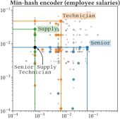
Figure 3: The min-hash encoder transforms containment into inequality operations. Color dots are categories that contain the corresponding colored substrings and gray dots are categories that do not contain any of them. The category Senior Supply Technician (black dot) is in the intersection of the three containment regions.

As an example, Figure 3 shows this global property of the min-hash encoder for the case of the employe salaries dataset with $d{=}2$. The substrings Senior, Supply and Technician are all included in the category Senior Supply Technician, and as consequence, the position for this category in the encoding space will be always in the intersection of the bottom-left regions generated by its substrings.

Finally, this encoder is specially suitable for very large scale settings, as it is very fast to compute and completely stateless. A stateless encoding is very useful for distributed computing: different workers can then process data simultaneously without communication. Its drawback is that, as it relies on hashing, the encoding cannot easily be inverted and interpreted in terms of the original string entries.

3.2 Gamma-Poisson factorization

To facilitate interpretation, we now introduce an encoding approach that estimates a decomposition of the string entries in terms of a linear combination of latent categories.

3.2.1 Model

We use a generative model of strings from latent categories. For this, we rely on the Gamma-Poisson model [28], a matrix factorization-technique well-suited to counting statistics. The idea was originally developed for finding low-dimensional representations, known as topics, of documents given their word count representation. As the string entries we consider are much shorter than text documents and can contain typos, we rely on their substring representation: we represent each observation by its count vector of character-level structure of n-grams. Each observation, a string entry described by its count vector $\mathbf{f}\in\mathbb{N}^{m}$, is modeled as a linear combination of $d$ unknown prototypes or topics, $\mathbf{\Lambda}\in\mathbb{R}^{d\times m}$:

$$\mathbf{f}\approx\mathbf{x}\,\mathbf{\Lambda},$$ (11)

Here, $\mathbf{x}\in\mathbb{R}^{d}$ are the activations that decompose the observation $\mathbf{f}$ in the prototypes $\mathbf{\Lambda}$ in the count space. As we will see later, these prototypes can be seen as latent categories.

Given a training dataset with $n$ samples, the model estimates the unknown prototypes $\mathbf{\Lambda}$ by factorizing the data’s bag-of-n-grams representation $\mathbf{F}\in\mathbb{N}^{n\times m}$, where $m$ is the number of different n-grams in the data:

$$\mathbf{F}\approx\mathbf{X}\,\mathbf{\Lambda},\quad\text{with }\mathbf{X}\in\mathbb{R}^{n\times d},\mathbf{\Lambda}\in\mathbb{R}^{d\times m}$$ (12)

As $\mathbf{f}$ is a vector of counts, it is natural to consider a Poisson distribution for each of its elements:

$$p\bigl{(}f_{j}|(\mathbf{x}\,\mathbf{\Lambda})_{j}\bigr{)}=\frac{1}{f_{j}!}(\mathbf{x}\,\mathbf{\Lambda})_{j}^{f_{j}}e^{-(\mathbf{x}\,\mathbf{\Lambda})_{j}},\quad j=1,...,m.$$ (13)

For a prior on the elements of $\mathbf{x}\in\mathbb{R}^{d}$, we use a Gamma distribution, as it is the conjugate prior of the Poisson distribution, but also because it can foster a soft sparsity:

$$p(x_{i})=\frac{x_{i}^{\alpha_{i}-1}e^{-x_{i}/\beta_{i}}}{\beta_{i}^{\alpha_{i}}\,\Gamma(\alpha_{i})},\quad i=1,...,d,$$ (14)

where $\boldsymbol{\alpha}$, $\boldsymbol{\beta}$ $\in\mathbb{R}^{d}$ are the shape and scale parameters of the Gamma distribution for each one of the $d$ topics.

3.2.2 Estimation strategy

To fit the model to the input data, we maximize the log-likelihood of the model, written as:

$$\log\mathcal{L} = \quad\sum_{j=1}^{m}f_{j}\log((\mathbf{x}\,\mathbf{\Lambda})_{j})-(\mathbf{x}\,\mathbf{\Lambda})_{j}-\log(f_{j}!)\,+$$

$$\quad\sum_{i=1}^{d}(\alpha_{i}{-}1)\log(x_{i})-\frac{x_{i}}{\beta_{i}}-\alpha_{i}\log\beta_{i}-\log\Gamma(\alpha_{i})$$ (15)

Maximizing the log-likelihood with respect to the parameters gives:

$$\frac{\partial}{\partial\Lambda_{ij}}\log\mathcal{L} =\frac{f_{j}}{(\mathbf{x}\,\mathbf{\Lambda})_{j}}x_{i}-x_{i}$$ (16)

$$\frac{\partial}{\partial x_{i}}\log\mathcal{L} =\sum_{j=1}^{m}\frac{f_{j}}{(\mathbf{x}\,\mathbf{\Lambda})_{j}}\Lambda_{ij}-\Lambda_{ij}+\frac{\alpha_{i}-1}{x_{i}}-\frac{1}{\beta_{i}}$$ (17)

As explained in [28], these expressions are analogous to solving the following non-negative matrix factorization (NMF) with the generalized Kullback-Leibler divergence as loss:

$$\begin{pmatrix}\mathbf{F}\\ \text{diag}(\boldsymbol{\beta})^{-1}\end{pmatrix}=\mathbf{X}\begin{pmatrix}\mathbf{\Lambda}\\ \text{diag}(\boldsymbol{\alpha})-I_{d}\end{pmatrix}$$ (18)

In other words, the Gamma-Poisson model can be interpreted as a constrained non-negative matrix factorization in which the generalized Kullback-Leibler divergence is minimized between $\mathbf{F}$ and $\mathbf{X}\mathbf{\Lambda}$, subject to a Gamma prior in the distribution of the elements of $\mathbf{X}$. The Gamma prior induces sparsity in the activations $\mathbf{x}$ of the model.

To solve the NMF problem above, [36] proposes the following recurrences:

$$\Lambda_{ij} \leftarrow\Lambda_{ij}\left(\sum_{\ell=1}^{n}\frac{f_{\ell j}}{(\mathbf{X}\mathbf{\Lambda})_{\ell j}}x_{\ell i}\right)\left(\sum_{\ell=1}^{n}x_{\ell i}\right)^{-1}$$ (19)

$$x_{\ell i} \leftarrow x_{\ell i}\left(\sum_{j=1}^{m}\frac{f_{\ell j}}{(\mathbf{X}\mathbf{\Lambda})_{\ell j}}\Lambda_{ij}+\frac{\alpha_{i}-1}{x_{\ell i}}\right)\left(\sum_{j=1}^{m}\Lambda_{ij}+\beta_{i}^{-1}\right)^{-1}$$ (20)

As $\mathbf{F}$ is a sparse matrix, the summations above only need to be computed on the non-zero elements of $\mathbf{F}$. This fact considerably decreases the computational cost of the algorithm.

Input : $\mathbf{F}{\in}\mathbb{R}^{n\times m},\mathbf{\Lambda}^{(0)}{\in}\mathbb{R}^{d\times m},\boldsymbol{\alpha},\boldsymbol{\beta}\in\mathbb{R}^{d},\rho,q,\eta,\epsilon$

Output : $\mathbf{X}{\in}\mathbb{R}^{n\times d},\mathbf{\Lambda}{\in}\mathbb{R}^{d\times m}$

1 while  $\lVert\mathbf{\Lambda}^{(t)}-\mathbf{\Lambda}^{(t-1)}\rVert_{F}>\eta$ do

2       draw $\mathbf{f}_{t}$ from the training set $\mathbf{F}$.

3       while  $\lVert\mathbf{x}_{t}-\mathbf{x}_{t}^{\text{old}}\rVert_{2}>\epsilon$ do

4             $\mathbf{x}_{t}\leftarrow\left[\mathbf{x}_{t}\left(\frac{\mathbf{f}_{t}}{\mathbf{x}_{t}\mathbf{\Lambda}^{(t)}}\right)\mathbf{\Lambda}^{(t)\mathsf{T}}+\boldsymbol{\alpha}-1\right].\left[\mathbf{1}\,\mathbf{\Lambda}^{(t)\mathsf{T}}{+}\boldsymbol{\beta}^{-1}\right]^{.-1}$

5       end while

6       $\mathbf{\tilde{A}}_{t}\leftarrow\mathbf{\Lambda}^{(t)}.\left[\mathbf{x}_{t}^{\mathsf{T}}\left(\frac{\mathbf{f}_{t}}{\mathbf{x}_{t}\mathbf{\Lambda}^{(t)}}\right)\right]$

7       $\mathbf{\tilde{B}}_{t}\leftarrow\mathbf{x}_{t}^{\mathsf{T}}\mathbf{1}$

       if $t\equiv 0\bmod q$,

        // Every $q$ iterations

8       then

9             $\mathbf{A}^{(t)}\leftarrow\rho\,\mathbf{A}^{(t-q)}+\sum_{s=t-q+1}^{t}\mathbf{\tilde{A}}^{(s)}$

10             $\mathbf{B}^{(t)}\leftarrow\rho\,\mathbf{B}^{(t-q)}+\sum_{s=t-q+1}^{t}\mathbf{\tilde{B}}^{(s)}$

11             $\mathbf{\Lambda}^{(t)}\leftarrow\mathbf{A}^{(t)}./\,\mathbf{B}^{(t)}$

12            

13       end if

14       $t\leftarrow t+1$

15      

16 end while

Algorithm 1 Online Gamma-Poisson factorization

Following [37], we present an online (or streaming) version of the Gamma-Poisson solver (algorithm 1). The algorithm exploits the fact that in the recursion for $\mathbf{\Lambda}$ (eq. 19 and 20), the summations are done with respect to the training samples. Instead of computing the numerator and denominator in the entire training set at each update, one can update them only with mini-batches of data, which considerably decreases the memory usage and time of the computations.

For better computational performance, we adapt the implementation of this solver to the specificities of our problem—factorizing substring counts across entries of a categorical variable. In particular, we take advantage of the repeated entries by saving a dictionary of the activations for each category in the convergence of the previous mini-batches (algorithm 1, line 4) and use them as an initial guess for the same category in a future mini-batch. This is a warm restart and is especially important in the case of categorical variables because for most datasets, the number of unique categories is much lower than the number of samples.

We also set the hyper-parameters of the algorithm and its initialization for optimal convergence. For $\rho$, the discount factor for the previous iterations of the topic matrix $\mathbf{\Lambda}^{(t)}$ (algorithm 1, line 9-10). choosing $\rho{=}0.95$ gives good convergence speed while avoiding instabilities (Figure 10 in the Appendix). With respect to the initialization of the topic matrix $\mathbf{\Lambda}^{(0)}$, a good option is to choose the centroids of a k-means clustering (Figure 11) in a hashed version of the n-gram count matrix $\mathbf{F}$ and then use as initializations the nearest neighbor observations in the original n-gram space. In the case of a streaming setting, the same approach can be used in a subset of the data.

3.2.3 Inferring feature names

An encoding strategy where each dimension can be understood by humans facilitates the interpretation of the full statistical analysis. A straightforward strategy for interpretation of the Gamma Poisson encoder is to describe each encoding dimension by features of the string entries that it captures. For this, one alternative is to track the feature maps corresponding to each input category, and assign labels based on the input categories that activate the most in a given dimensionality. Another option is to apply the same strategy, but for substrings, such as words contained in the input categories. In the experiments, we follow the second approach as a lot of datasets are composed of entries with overlap, hence individual words carry more information for interpretability than the entire strings.

This method is expected to work well if the encodings are sparse and composed only of non-negative values with a meaningful magnitude. The Gamma-Poisson factorization model ensures these properties.

TABLE III: Non-curated datasets. Description for the corresponding high-cardinality categorical variable.

Dataset	#samples	#categories	#categories per 1000 samples	Gini coefficient	Mean category length (#chars)	Source of high cardinality
Crime Data	1.5M	135	64.5	0.85	30.6	Multi-label
Medical Charges	163k	100	99.9	0.23	41.1	Multi-label
Kickstarter Projects	281k	158	123.8	0.64	11.0	Multi-label
Employee Salaries	9.2k	385	186.3	0.79	24.9	Multi-label
Open Payments	2.0M	1.4k	231.9	0.90	24.7	Multi-label
Traffic Violations	1.2M	11.3k	243.5	0.97	62.1	Typos; Description
Vancouver Employees	2.6k	640	341.8	0.67	21.5	Multi-label
Federal Election	3.3M	145.3k	361.7	0.76	13.0	Typos; Multi-label
Midwest Survey	2.8k	844	371.9	0.67	15.0	Typos
Met Objects	469k	26.8k	386.1	0.88	12.2	Typos; Multi-label
Drug Directory	120k	17.1k	641.9	0.81	31.3	Multi-label
Road Safety	139k	15.8k	790.1	0.65	29.0	Multi-label
Public Procurement	352k	28.9k	804.6	0.82	46.8	Multi-label; Multi-language
Journal Influence	3.6k	3.2k	956.9	0.10	30.0	Multi-label; Multi-language
Building Permits	554k	430.6k	940.0	0.48	94.0	Typos; Description
Wine Reviews	138k	89.1k	997.7	0.23	245.0	Description
Colleges	7.8k	6.9k	998.0	0.02	32.1	Multi-label

4 Experimental study

We now study experimentally different encoding methods in terms of interpretability and supervised-learning performance. For this purpose, we use three different types of data: simulated categorical data, and real data with curated and non-curated categorical entries.

We benchmark the following strategies: one-hot, tf-idf, fastText [38], Bert [26], similarity encoding [7], the Gamma-Poisson factorization, and min-hash encoding. For all the strategies based on a n-gram representation, we use the set of 2-4 character grams. For a fair comparison across encoding strategies, we use the same dimensionality $d$ in all approaches. To set the dimensionality of one-hot encoding, tf-idf and fastText, we used a truncated SVD (implemented efficiently following [39]). Note that dimensionality reduction improves one-hot encoding with tree-based learners for data with rare categories [7]. For similarity encoding, we select prototypes with a k-means strategy, as it gives slightly better prediction results than the most frequent categories.

4.1 Real-life datasets with string categories

4.1.1 Datasets with high-cardinality categories

In order to evaluate the different encoding strategies, we collected 17 real-world datasets containing a prediction task and at least one relevant high-cardinality categorical variable as feature. subsubsection 3.2.3 shows a quick description of the datasets and the corresponding categorical variables (see Appendix A.1.1 for a description of datasets and the related learning tasks). subsubsection 3.2.3 also details the source of high-cardinality for the datasets: multi-label, typos, description and multi-language. We call multi-label the situation when a single column contains multiple information shared by several entries, e.g., supply technician, where supply denotes the type of activity, and technician denotes the rank of the employee (as opposed, e.g., to manager). Typos refers to entries having small morphological variations, as midwest and mid-west. Description refers to categorical entries that are composed of a short free-text description. These are close to a typical NLP problem, although constrained to a very particular subject, so they tend to contain very recurrent informative words and near-duplicate entries. Finally, multi-language are datasets in which the categorical variable contains more that one language across the different entries.

4.1.2 Datasets with curated strings

We also evaluate encoders when the categorical variables have already been curated: often, entries are standardized to create low-cardinality categorical variables. For this, we collected seven of such datasets (see Appendix A.1.2). On these datasets we study the robustness of the n-gram based approaches to situations where there is no a priori need to reduce the dimensionality of the problem.

4.2 Recovering latent categories

4.2.1 Recovery on simulated data

subsubsection 3.2.3 shows that the most common scenario for high-cardinality string variables are multi-label categories. The second most common problem is the presence of typos (or any source of morphological variation of the same idea). To analyze these two cases in a controlled setting, we create two simulated sets of categorical variables. Table IV shows examples of generated categories, taking as a base 8 ground-truth categories of animals (details in Appendix A.3).

To measure the ability of an encoder to recover a feature matrix close to a one-hot encoding matrix of ground-truth categories in these simulated settings, we use the Normalized Mutual Information (NMI) as metric. Given two random variables $X_{1}$ and $X_{2}$, the NMI is defined as:

$$\text{NMI}=2\,\frac{I(X_{1};X_{2})}{H(X_{1})+H(X_{2})}$$ (21)

Where $I(\cdot\,;\cdot)$ is the mutual information and $H(\cdot)$ the entropy. To apply this metric to the feature matrix $\mathbf{X}$ generated by the encoding of all ground truth categories, we consider $\mathbf{X}$ –after rescaling with an $\ell_{1}$ normalization of the rows– as a two dimensional probability distribution. For encoders that produce feature matrices with negative values, we take the element-wise absolute value of $\mathbf{X}$. The NMI is a classic measure of correspondences between clustering results [40]. Beyond its information-theoretical interpretation, an appealing property is that it is invariant to order permutations. The NMI of any permutation of the identity matrix is equal to 1 and the NMI of any constant matrix is equal to 0. Thus, the NMI in this case is interpreted as a recovering metric of a one-hot encoded matrix of latent, ground truth, categories.

Table V shows the NMI for both simulated datasets. The Gamma-Poisson factorization obtains the highest values in both multi-label and typos settings and for different dimensionalities of the encoders. The best recovery is obtained when the dimensionality of the encoder is equal to the number of ground-truth categories, i.e., $d{=}8$.

TABLE IV: Examples of simulated categorical variables.

Type	Example categories
Ground truth	chicken; eagle; giraffe; horse; leopard;
	lion; tiger; turtle.
Multi-label	lion chicken; horse eagle lion.
Typos (10%)	itger; tiuger; tgier; tiegr; tigre; ttiger.

TABLE V: Recovery of categories for simulations: Normalized mutual information (NMI) for different encoders.

Encoder	Multi-label			Typos
	$d$=6	$\mathbf{d}$=8	$d$=10	$d$=6	$\mathbf{d}$=8	$d$=10
Tf-idf + SVD	0.16	0.18	0.17	0.17	0.16	0.16
FastText + SVD	0.08	0.09	0.09	0.07	0.08	0.08
Bert + SVD	0.03	0.03	0.03	0.05	0.06	0.06
Similarity Encoder	0.32	0.25	0.24	0.72	0.82	0.80
Min-hash Encoder	0.14	0.15	0.13	0.14	0.15	0.13
Gamma-Poisson	0.76	0.82	0.79	0.77	0.83	0.80

4.2.2 Results for real curated data

TABLE VI: Recovering true categories for curated entries. NMI for different encoders ($d$=30) – Appendix C gives results for different dimensions.

Dataset	Gamma	Similarity	Tf-idf	FastText	Bert
(cardinality)	Poisson	Encoding	+ SVD	+ SVD	+ SVD
Adult (15)	0.75	0.71	0.54	0.19	0.07
Cacao Flavors (100)	0.51	0.30	0.28	0.07	0.04
California Housing (5)	0.46	0.51	0.56	0.20	0.05
Dating Profiles (19)	0.52	0.24	0.25	0.12	0.05
House Prices (15)	0.83	0.25	0.32	0.11	0.05
House Sales (70)	0.42	0.04	0.18	0.06	0.02
Intrusion Detection (66)	0.34	0.58	0.46	0.11	0.05

For curated data, the cardinality is usually low. We nevertheless perform the encoding using a default choice of $d=30$, to gauge how well turn-key generic encoding represent these curated strings. Table VI shows the NMI values for the different curated datasets, measuring how much the generated encoding resembles a one-hot encoding on the curated categories. Despite the fact that it is used with a dimensionality larger than the cardinality of the curated category, Gamma-Poisson factorization has the highest recovery performance in 5 out of 7 datasets.

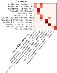
(a) Employee Salaries dataset (Occupation)

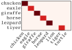
(b) Simulated typos

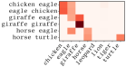
(c) Simulated multi-label categories

Figure 4: Gamma-Poisson factorization gives positive and sparse representations that are easily interpretable. Examples of encoding vectors (d=8) for a real dataset (a) and for simulated data (b and c) obtained with a Gamma-Poisson factorization. The $x$-axis shows the activations for each dimension with their respective inferred feature names. Figure 14 in the Appendix shows that other encoders fail to give such an easily-understandable picture.

These experiments show that Gamma-Poisson factorization recovers well latent categories. To validate this intuition, Figure 4 shows such encodings in the case of the simulated data as well as the real-world non-curated Employees Salaries dataset. It confirms that the encodings can be interpreted as loadings on discovered categories that match the inferred feature names.

4.3 Encoding for supervised learning

We now study the encoders for statistical analysis by measuring prediction accuracy in supervised-learning tasks.

4.3.1 Experiment settings

We use gradient boosted trees, as implemented in XGBoost [41]. Note that trees can be implemented on categorical variables. However, this encounter the same problems as one-hot encoding: the number of comparisons grows with the number of categories. Hence, the best trees approaches for categorical data use target encoding to impose an order on categories [42]. We also investigated other supervised-learning approaches: linear models, multilayer perceptron, and kernel machines with RBF and polynomial kernels. However, even with significant hyper-parameter tuning, they under-performed XGBoost on our tabular datasets (Figure 13 in the Appendix). The good performance of gradient-boosted trees is consistent with previous reports of systematic benchmarks [43].

Depending on the dataset, the learning task can be either regression, binary or multiclass classification. As datasets get different prediction scores, we visualize encoders’ performance with prediction results scaled in a relative score. It is a dataset-specific scaling of the original score, in order to bring performance across datasets in the same range. In other words, for a given dataset $i$:

$$\text{relative score}^{i}_{j}=100\frac{\text{score}^{i}_{j}-\min_{j}{\text{score}^{i}_{j}}}{\max_{j}{\text{score}^{i}_{j}}-\min_{j}{\text{score}^{i}_{j}}}$$ (22)

where $\text{score}^{i}_{j}$ is the the prediction score for the dataset $i$ with the configuration $j{\in}\mathcal{J}$, the set of all trained models—in terms of dimensionality, type of encoder and cross-validation split. The relative score is figure-specific and is only intended to be used as a visual comparison of classifiers’ performance across multiple datasets. A higher relative score means better results.

For a proper statistical comparison of encoders, we use a ranking test across multiple datasets [44]. Note that in such a test each dataset amounts to a single sample, and not the cross-validation splits which are not mutually independent. To do so, for a particular dataset, encoders were ranked according to the median score value over cross-validation splits. At the end, a Friedman test [45] is used to determine if all encoders, for a fixed dimensionality $d$, come from the same distribution. If the null hypothesis is rejected, we use a Nemenyi post-hoc test [46] to verify whether the difference in performance across pairs of encoders is significant.

To do pairwise comparison between two encoders, we use a pairwise Wilcoxon signed rank test. The corresponding p-values rejects the null hypothesis that the two encoders are equally performing across different datasets.

4.3.2 Prediction with non-curated data

We now describe the results of several prediction benchmarks with the 17 non-curated datasets.

First, note that one-hot, tf-idf and fastText are naturally high-dimensional encoders, so a dimensionality reduction technique needs to be applied in order to compare the different methodologies—also, without this reduction, the benchmark will be unfeasible given the long computational times of gradient boosting. Moreover, dimensionality reduction helps to improve prediction (see [7]) with tree-based methods. To approximate Euclidean distances, SVD is optimal. However, it has a cost of $nd\min(n,d)$. Using Gaussian random projections [47] is appealing, as can lead to stateless encoders that requires no fit. Table VII compares the prediction performance of both strategies. For tf-idf and fastText, the SVD is significantly superior to random projections. On the contrary, there is no statistical difference for one-hot, even though the performance is slightly superior for the SVD (p-value equal to 0.492). Given these results, we use SVD for all further benchmarks.

TABLE VII: Comparing SVD and Gaussian random projection as a dimensionality reduction Wilcoxon test p-values for different encoders. Prediction performance with SVD is significantly superior for tf-idf, FastText and Bert.

Encoder	SVD v/s Random projection (p-value)
Tf-idf	0.001
FastText	0.006
Bert	0.001
One-hot	0.717

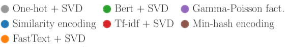
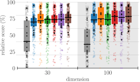
Figure 5: Encoding with subword information performs significantly better than one-hot. Classifier: XGBoost. Comparison of encoders in terms of a relative score (the prediction score on the particular dataset, rescaled with respect to the global maximum and minimum score values across dimensions). Color dots indicate the scores for each cross-validation fold, black dots the median score across folds for a dataset, the black line indicates the median score and the box gives the interquartile range.

Figure 5 compares encoders in terms of the relative score of Equation 22. All n-gram based encoders clearly improve upon one-hot encoding, at both dimensions ($d$ equal to 30 and 100). Min-hash gives a slightly better prediction performance across datasets, despite of being the only method that does not require a data fit step. The Nemenyi ranking test confirms the visual impression: n-gram-based methods are superior to one-hot encoding; and the min-hash encoder has the best average ranking value for both dimensionalities, although the difference in prediction with respect to the other n-gram based methods is not statistically significant.

While we seek generic encoding approaches, using precomputed embeddings requires the choice of a language. As 15 out of 17 datasets are fully in English, the benchmarks above use English embeddings for fastText. Figure 6, studies the importance of this choice, comparing the prediction results for fastText in different languages (English, French and Hungarian). Not choosing English leads to a sizeable drop in prediction accuracy, which gets bigger for languages more distant (such as Hungarian). This shows that the natural language semantics of fastText indeed are important to explain its good prediction performance. A good encoding not only needs to represent the data in a low dimension, but also to capture the similarities between the different entries.

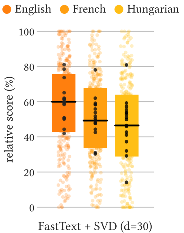
Figure 6: FastText prediction performance drops languages other than English. Relative prediction scores with pretrained fastText vectors in different languages. The dimensionality was set with an SVD. A pairwise Wilcoxon signed rank tests give the following p-values:
English-French $p$=0.056, French-Hungarian $p$=0.149, English-Hungarian $p$=0.019.

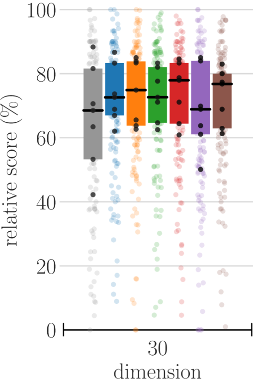
Figure 7: All encoders perform well for low-cardinality datasets. Classifier: XGBoost. The score is relative to the best and worse prediction across datasets (Equation 22). Color dots indicate the scores for each cross-validation fold, black dots the median across folds, the black line indicates the median across datasets and the box gives the interquartile range. Differences are not significant.

4.3.3 Prediction with curated data

We now test the robustness of the different encoding methods to situations where there is no need to capture subword information—e.g., low cardinality categorical variables, or variables as ”Country name”, where the overlap of character n-grams does not have a relevant meaning. We benchmark in Figure 7 all encoders on 7 curated datasets. To simulate black-box usage, the dimensionality was fixed to $d{=}30$ for all of them, with the exception of one-hot. None of the n-gram based encoders perform worst than one-hot. Indeed, the F statistics for the average ranking does not reject the null hypothesis of all encoders coming from the same distribution (p-value equal to 0.37).

4.3.4 Interpretable data science with the Gamma-Poisson

As shown in Figure 4, the Gamma-Poisson factorization creates sparse, non-negative feature vectors that are easily interpretable as a linear combination of latent categories. We give informative features names to each of these latent categories (see 3.2.3). To illustrate how such encoding can be used in a data-science setting where humans need to understand results, Figure 8 shows the permutation importances [48] of each encoding direction of the Gamma-Poisson factorization and its corresponding feature names. By far, the most important inferred feature name to predict salaries in the Employee Salaries dataset is the latent category Manager, Management, Property, which matches general intuitions on salaries.

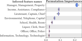
Figure 8: Gamma-Poisson enables interpretable data science. The box plots display permutation importances for the variable Employee Position Title in the Employee Salaries dataset. Here we show the 8 most important latent topics from a total of 30. The overall feature importances for every feature in the dataset are shown in Figure 12 in the Appendix.

5 Discussion and conclusion

One-hot encoding is not well suited to columns of a table containing categories represented with many different strings [7]. Character n-gram count vectors can represent strings well, but they dilute the notion of categories with extremely high-dimensional vectors. A good encoding should capture string similarity between entries and reflect it in a lower dimensional encoding.

We study several encoding approaches to capture the structural similarities of string entries. The min-hash encoder gives a stateless representation of strings to a vector space, transforming inclusions between strings into simple inequalities (Theorem 3.1). A Gamma-Poisson factorization on the count matrix of sub-strings gives a low-rank approximation of similarities.

Scalability

Both Gamma-Poisson factorization and the min-hash encoder can be used on very large datasets, as they work in streaming settings. They markedly improve upon one-hot encoder for large scale-learning as i) they do not need the definition of a vocabulary, ii) they give low dimensional representations, and thus decrease the cost of subsequent analysis steps. Indeed, for both of these encoding approaches, the cost of encoding is usually significantly smaller than that of running a powerful supervised learning method such as XGBoost, even on the reduced dimensionality (Appendix C in the Appendix). The min-hash encoder is unique in terms of scalability, as it gives low-dimensional representations while being completely stateless, which greatly facilitates distributed computing. The representations enable much better statistical analysis than a simpler stateless low-dimensional encoding built with random projections of n-gram string representations. Notably, the most scalable encoder is also the best performing for supervised learning, at the cost of some loss in interpretability.

Recovery of latent categories

Describing results in terms of a small number of categories can greatly help interpreting a statistical analysis. Our experiments on real and simulated data show that encodings created by the Gamma-Poisson factorization correspond to loadings on meaningful recovered categories. It removes the need to manually curate entries to understand what drives an analysis. For this, positivity of the loadings and the soft sparsity imposed by the Gamma prior is crucial; a simple SVD fails to give interpretable loadings (Appendix Figure 14).

AutoML settings

AutoML (automatic machine learning) strives to develop machine-learning pipeline that can be applied to datasets without human intervention [49, 50]. To date, it has focused on tuning and model selection for supervised learning on numerical data. Our work addresses the feature-engineering step. In our experiments, we apply the exact same prediction pipeline to 17 non-curated and 7 curated tabular datasets, without any custom feature engineering. Both Gamma-Poisson factorization and min-hash encoder led to best-performing prediction accuracy, using a classic gradient-boosted tree implementation (XGBoost). We did not tune hyper-parameters of the encoding, such as dimensionality or parameters of the priors for the Gamma Poisson. They adapt to the language and the vocabulary of the entries, unlike NLP embeddings such as fastText which must have been previously extracted on a corpus of the language (Figure 6). These string categorical encodings therefore open the door to autoML on the original data, removing the need for feature engineering which can lead to difficult model selection. A possible rule when integrating tabular data into an autoML pipeline could be to apply min-hash or Gamma-Poisson encoder for string categorical columns with a cardinality above 30, and use one-hot encoding for low-cardinality columns. Indeed, results show that these encoders are also suitable for normalized entries.

One-hot encoding is the defacto standard for statistical analysis on categorical entries. Beyond its simplicity, its strength is to represent the discrete nature of categories. However, it becomes impractical when there are too many different unique entries, for instance because the string representations have not been curated and display typos or combinations of multiple informations in the same entries. For high-cardinality string categories, we have presented two scalable approaches to create low-dimensional encoding that retain the qualitative properties of categorical entries. The min-hash encoder is extremely scalable and gives the best prediction performance because it transforms string inclusions to vector-space operations that can easily be captured by a supervised learning step. If interpretability of results is an issue, the Gamma-Poisson factorization performs almost as well for supervised learning, but enables expressing results in terms of meaningful latent categories. As such, it gives a readily-usable replacement to one-hot encoding for high-cardinality string categorical variables. Progress brought by these encoders is important, as they avoid one of the time-consuming steps of data science: normalizing entries of databases via human-crafted rules.

Acknowledgments

Authors were supported by the DirtyData (ANR-17-CE23-0018-01) and the FUI Wendelin projects.

Patricio Cerda Patricio holds a masters degree in applied mathematics from École Normale Supérieure Paris-Saclay and a PhD in computer science from Université Paris-Saclay. His research interests are natural language processing, econometrics and causality.s

Gaël Varoquaux Gaël Varoquaux is a research director at Inria developing statistical learning for data science and scientific inference. He has pioneered machine learning on brain images. More generally, he develops tools to make machine learning easier, for real-life, uncurated data. He co-funded scikit-learn and helped build central tools for data analysis in Python. He has a PhD in quantum physics and graduated from École Normale Supérieure Paris.

Appendix A Reproducibility

A.1 Dataset Description

A.1.1 Non-curated datasets

Building Permits (sample size: 554k). Permits issued by the Chicago Department of Buildings since 2006. Target (regression): Estimated Cost. Categorical variable: Work Description (cardinality: 430k).

Colleges (7.8k). Information about U.S. colleges and schools. Target (regression): Percent Pell Grant. Cat. var.: School Name (6.9k).

Crime Data (1.5M). Incidents of crime in the City of Los Angeles since 2010. Target (regression): Victim Age. Categorical variable: Crime Code Description (135).

Drug Directory (120k). Product listing data submitted to the U.S. FDA for all unfinished, unapproved drugs. Target (multiclass): Product Type Name. Categorical var.: Non Proprietary Name (17k).

Employee Salaries (9.2k). Salary information for employees of the Montgomery County, MD. Target (regression): Current Annual Salary. Categorical variable: Employee Position Title (385).

Federal Election (3.3M). Campaign finance data for the 2011-2012 US election cycle. Target (regression): Transaction Amount. Categorical variable: Memo Text (17k).

Journal Influence (3.6k). Scientific journals and the respective influence scores. Target (regression): Average Cites per Paper. Categorical variable: Journal Name (3.1k).

Kickstarter Projects (281k). More than 300,000 projects from https://www.kickstarter.com. Target (binary): State. Categorical variable: Category (158).

Medical Charges (163k). Inpatient discharges for Medicare beneficiaries for more than 3,000 U.S. hospitals. Target (regression): Average Total Payments. Categorical var.: Medical Procedure (100).

Met Objects (469k). Information on artworks objects of the Metropolitan Museum of Art’s collection. Target (binary): Department. Categorical variable: Object Name (26k).

Midwest Survey (2.8k). Survey to know if people self-identify as Midwesterners. Target (multiclass): Census Region (10 classes). Categorical var.: What would you call the part of the country you live in now? (844).

Open Payments (2M). Payments given by healthcare manufacturing companies to medical doctors or hospitals (year 2013). Target (binary): Status (if the payment was made under a research protocol). Categorical var.: Company name (1.4k).

Public Procurement (352k). Public procurement data for the European Economic Area, Switzerland, and the Macedonia. Target (regression): Award Value Euro. Categorical var.: CAE Name (29k).

Road Safety (139k). Circumstances of personal injury of road accidents in Great Britain from 1979. Target (binary): Sex of Driver. Categorical variable: Car Model (16k).

Traffic Violations (1.2M). Traffic information from electronic violations issued in the Montgomery County, MD. Target (multiclass): Violation type (4 classes). Categorical var.: Description (11k).

Vancouver Employee(2.6k). Remuneration and expenses for employees earning over $75,000 per year. Target (regression): Remuneration. Categorical variable: Title (640).

Wine Reviews (138k). Wine reviews scrapped from WineEnthusiast. Target (regression): Points. Categorical variable: Description (89k).

A.1.2 Curated datasets

Adult (sample size: 32k). Predict whether income exceeds $50K/yr based on census data. Target (binary): Income. Categorical variable: Occupation (cardinality: 15).

Cacao Flavors (1.7k). Expert ratings of over 1,700 individual chocolate bars, along with information on their origin and bean variety. Target (multiclass): Bean Type. Categorical variable: Broad Bean Origin (100).

California Housing (20k). Based on the 1990 California census data. It contains one row per census block group (a block group typically has a population of 600 to 3,000 people). Target (regression): Median House Value. Categorical variable: Ocean Proximity (5).

Dating Profiles (60k). Anonymized data of dating profiles from OkCupid. Target (regression): Age. Categorical variable: Diet (19).

House Prices (1.1k). Contains variables describing residential homes in Ames, Iowa. Target (regression): Sale Price. Categorical variable: MSSubClass (15).

House Sales (21k). Sale prices for houses in King County, which includes Seattle. Target (regression): Price. Categorical variable: ZIP code (70).

Intrusion Detection (493k). Network intrusion simulations with a variaty od descriptors of the attack type. Target (multiclass): Attack Type. Categorical variable: Service (66).

A.2 Learning pipeline

Sample size

Datasets’ size range from a couple of thousand to several million samples. To reduce computation time on the learning step, the number of samples was limited to 100k for large datasets.

Data preprocessing

We removed rows with missing values in the target or in any explanatory variable other than the selected categorical variable, for which we replaced missing entries by the string ‘nan’. The only additional preprocessing for the categorical variable was to transform all entries to lower case.

Cross-validation

For every dataset, we made 20 random splits of the data, with one third of samples for testing at each time. In the case of binary classification, we performed stratified randomization.

Performance metrics

Depending on the type of prediction task, we used different scores to evaluate the performance of the supervised learning problem: for regression, we used the $R^{2}$ score; for binary classification, the average precision; and for multi-class classification, the accuracy score.

Parametrization of classifiers

We used the scikit-learn [51] for most of the data processing. For all the experiments, we used the scikit-learn compatible implementations of XGBoost [41], with a grid search on the learning_rate (0.05, 0.1, 0.3) and max_depth (3, 6, 9) parameters. All datasets and encoders use the same parametrization.

Dimensionality reduction

We used the scikit-learn implementations of TruncatedSVD and GaussianRandomProjection, with the default parametrization in both cases.

A.3 Synthetic data generation

Multi-label categories

The multi-label data was created by concatenating $k{+}2$ ground truth categories (labels), with $k$ following a Poisson distribution—hence, all entries contain at least two concatenated labels. Not having single labels in the synthetic data makes the recovering of latent categories harder.

Typo generator

For the simulation of typos, we added 10% of variations of the original ground truth categories by adding errors randomly (missing, swaped, inserted and replaced characters). For each ground-truth category, a list of misspelled candidates (at least 15 per category) was obtained from the website: https://www.dcode.fr/typing-error-generator. Then, the misspelled categories were randomly chosen to generate the 10% of typos.

A.4 Online Resources

Experiments are available in Python code at https://github.com/pcerda/string_categorical_encoders. Implementations and examples on learning with string categories can be found at http://dirty-cat.github.io. The available encoders are compatible with the scikit-learn’s API.

Appendix B Algorithmic considerations

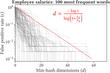
Figure 9: Number of dimensions required to identify inclusions. Grey lines are the proportion of false positives obtained for the 100 most frequent words in the employee salaries dataset ($H_{0}$ corresponds to identifying categories that do not contain the given word). The red line represents the theoretical minimum dimensionality required to obtain a desired false positive rate (with $k_{x}{/}k_{y}=0.125$, the inverse of the maximum number of words per category), as shown in Theorem 3.1.

B.1 Gamma-Poisson factorization

TABLE VIII: Parameter values for the Gamma-Poisson factorization. The same parameters were used for all datasets.

Parameter	Definition	Default value
$\alpha_{i}$	Poisson shape	1.1
$\beta_{i}$	Poisson scale	1.0
$\rho$	Discount factor	0.95
$q$	Mini-batch size	256
$\eta$	Approximation error	$10^{-4}$
$\epsilon$	Approximation error	$10^{-3}$

Algorithm 1 requires some input parameters and initializations that can affect convergence. One important parameter is $\rho$, the discount factor for the fitting in the past. Figure 10 shows that choosing $\rho{=}.95$ gives the best compromise between stability of the convergence and data fitting in terms of the Generalized KL divergence. The default values used in the experiments are listed in Table VIII.

With respect to the initialization of the topic matrix $\mathbf{\Lambda}^{(0)}$, the best option is to choose the centroids of a k-means clustering (Figure 11) in a hashed version of the n-gram count matrix $\mathbf{F}$ in a reduced dimensionality (in order to speed-up convergence of the k-means algorithm) and then project back to the n-gram space with a nearest neighbors algorithm.

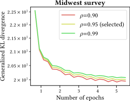
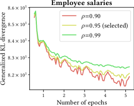
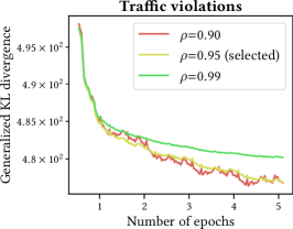
Figure 10: Convergence for different discount factor values for the Gamma-Poisson model. In all experiments, the value $\rho=0.95$ is used, as it gives a good trade-off between convergence and stability of the solution across the number of epochs.

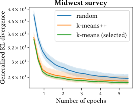
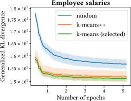
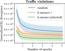
Figure 11: Convergence for different initializations for the Gamma-Poisson model. In all experiments, the k-means strategy is used.

Appendix C Additional figures and tables

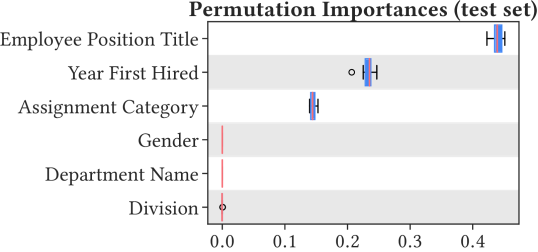
Figure 12: Overall permutation importances for every feature in the Employee Salaries dataset.

(a) One-hot encoder

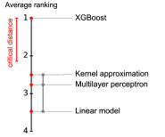
(b) Gamma-Poisson factorization

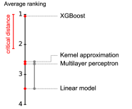
(c) Min-hash encoder

Figure 13: Comparison of classifiers against each other with the Nemenyi post-hoc test. Groups of classifiers that are not significantly different (at $\alpha$=0.05) are connected with a continuous gray line. The red line represents the value of the critical difference for rejecting the null hypothesis. The benchmarked classifiers are: XGBoost; Polynomial kernel approx. with the Nystroem method, followed by an $\ell 2$ regularized linear/logistic regression (kernel approximation); a multilayer perceptron (1-2 layers); and a $\ell 2$ regularized linear/logistic regression (linear model).

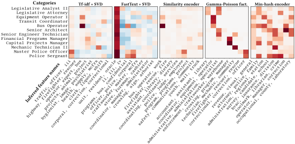
(a) Employee Position Title (Employee Salaries dataset)

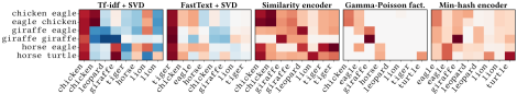
(b) Simulated multi-label entries

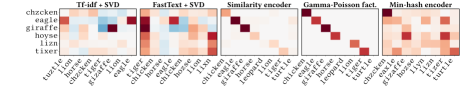
(c) Simulated entries with typos

Figure 14: The Gamma-Poisson factorization gives positive and sparse representations that are easily interpretable. Encoding vectors (d=8) for simulated (a and b) and a real dataset (c) obtained with different encoding methods for some categories ($y$-axis). The $x$-axis shows the activations with their respective inferred feature names.

TABLE IX: Median scores by dataset for XGBoost (d=30).

TABLE X: Median training and encoding times, in seconds, for Gamma-Poisson with XGBoost (d=30, a single fit, no hyper-parameter selection procedure).

TABLE XI: Recovering true categories for curated categorical variables. NMI for different encoders ($d{=}|C|$).

Dataset	Gamma-	Similarity	Tf-idf	FastText	Bert
(cardinality)	Poisson	Encoding	+ SVD	+ SVD	+ SVD
Adult (15)	0.84	0.71	0.54	0.19	0.07
Cacao Flavors (100)	0.48	0.34	0.34	0.1	0.05
California Housing (5)	0.83	0.51	0.56	0.20	0.05
Dating Profiles (19)	0.47	0.26	0.29	0.12	0.06
House Prices (15)	0.91	0.25	0.32	0.11	0.05
House Sales (70)	0.29	0.03	0.26	0.07	0.03
Intrusion Detection (66)	0.27	0.65	0.61	0.13	0.06

TABLE XII: Recovering true categories for curated entries. NMI for different encoders ($d$=10).

Dataset	Gamma	Similarity	Tf-idf	FastText	Bert
(cardinality)	Poisson	Encoding	+ SVD	+ SVD	+ SVD
Adult (15)	0.73	0.61	0.41	0.14	0.05
Cacao Flavors (100)	0.44	0.28	0.21	0.05	0.03
California Housing (5)	0.63	0.51	0.56	0.20	0.05
Dating Profiles (19)	0.34	0.28	0.20	0.08	0.03
House Prices (15)	0.81	0.26	0.26	0.09	0.04
House Sales (70)	0.49	0.04	0.11	0.05	0.02
Intrusion Detection (66)	0.34	0.53	0.46	0.08	0.04

TABLE XIII: Recovering true categories for curated entries. NMI for different encoders ($d$=100).

Dataset	Gamma	Similarity	Tf-idf	FastText	Bert
(cardinality)	Poisson	Encoding	+ SVD	+ SVD	+ SVD
Adult (15)	0.55	0.71	0.54	0.19	0.06
Cacao Flavors (100)	0.47	0.34	0.34	0.10	0.05
California Housing (5)	0.18	0.51	0.56	0.20	0.05
Dating Profiles (19)	0.30	0.26	0.29	0.12	0.06
House Prices (15)	0.63	0.25	0.32	0.11	0.05
House Sales (70)	0.21	0.03	0.26	0.07	0.03
Intrusion Detection (66)	0.23	0.65	0.61	0.13	0.06

References

- [1] J. Cohen, P. Cohen, S. West, and L. Aiken, Applied multiple regression/correlation analysis for the behavioral sciences. Routledge, 2013.
- [2] D. Pyle, Data preparation for data mining. Morgan Kaufmann, 1999.
- [3] E. Rahm and H. H. Do, “Data cleaning: Problems and current approaches,” IEEE Data Engineering Bulletin, vol. 23, p. 3, 2000.
- [4] W. E. Winkler, “Overview of record linkage and current research directions,” in Bureau of the Census. Citeseer, 2006.
- [5] A. K. Elmagarmid, P. G. Ipeirotis, and V. S. Verykios, “Duplicate record detection: A survey,” TKDE, vol. 19, p. 1, 2007.
- [6] P. Christen, Data matching: concepts and techniques for record linkage, entity resolution, and duplicate detection. Springer, 2012.
- [7] P. Cerda, G. Varoquaux, and B. Kégl, “Similarity encoding for learning with dirty categorical variables,” Machine Learning, 2018.
- [8] W. H. Gomaa and A. A. Fahmy, “A survey of text similarity approaches,” International Journal of Computer Applications, vol. 68, no. 13, pp. 13–18, 2013.
- [9] A. Gionis, P. Indyk, R. Motwani et al., “Similarity search in high dimensions via hashing,” in Vldb, vol. 99, no. 6, 1999, pp. 518–529.
- [10] D. Dheeru and E. Karra Taniskidou, “UCI machine learning repository,” 2017. [Online]. Available: http://archive.ics.uci.edu
- [11] W. Kim, B.-J. Choi, E.-K. Hong, S.-K. Kim, and D. Lee, “A taxonomy of dirty data,” Data mining and knowledge discovery, vol. 7, no. 1, pp. 81–99, 2003.
- [12] P. Oliveira, F. Rodrigues, and P. R. Henriques, “A formal definition of data quality problems,” in Proceedings of the 2005 International Conference on Information Quality (MIT IQ Conference), 2005.
- [13] L. Bottou and O. Bousquet, “The tradeoffs of large scale learning,” in NIPS, 2008, p. 161.
- [14] D. Micci-Barreca, “A preprocessing scheme for high-cardinality categorical attributes in classification and prediction problems,” ACM SIGKDD Explorations Newsletter, vol. 3, no. 1, pp. 27–32, 2001.
- [15] K. Weinberger, A. Dasgupta, J. Langford, A. Smola, and J. Attenberg, “Feature hashing for large scale multitask learning,” in ICML. ACM, 2009, p. 1113.
- [16] R. C. Angell, G. E. Freund, and P. Willett, “Automatic spelling correction using a trigram similarity measure,” Information Processing & Management, vol. 19, no. 4, pp. 255–261, 1983.
- [17] D. Klein, J. Smarr, H. Nguyen, and C. D. Manning, “Named entity recognition with character-level models,” in conference on Natural language learning at HLT-NAACL, 2003, p. 180.
- [18] J. Lu, C. Lin, J. Wang, and C. Li, “Synergy of database techniques and machine learning models for string similarity search and join,” in ACM International Conference on Information and Knowledge Management, 2019, p. 2975.
- [19] T. K. Landauer, P. W. Foltz, and D. Laham, “An introduction to latent semantic analysis,” Discourse processes, vol. 25, p. 259, 1998.
- [20] W. B. Johnson and J. Lindenstrauss, “Extensions of lipschitz mappings into a hilbert space,” Contemporary mathematics, vol. 26, no. 189-206, p. 1, 1984.
- [21] D. Achlioptas, “Database-friendly random projections: Johnson-lindenstrauss with binary coins,” Journal of computer and System Sciences, vol. 66, no. 4, pp. 671–687, 2003.
- [22] J. Pennington, R. Socher, and C. Manning, “Glove: Global vectors for word representation,” in EMNLP, 2014, pp. 1532–1543.
- [23] T. Mikolov, K. Chen, G. Corrado, and J. Dean, “Efficient estimation of word representations in vector space,” in ICLR, 2013.
- [24] S. Arora, Y. Liang, and T. Ma, “A simple but tough-to-beat baseline for sentence embeddings,” ICLR, 2017.
- [25] P. Bojanowski, E. Grave, A. Joulin, and T. Mikolov, “Enriching word vectors with subword information,” Transactions of the Association of Computational Linguistics, vol. 5, no. 1, pp. 135–146, 2017.
- [26] J. Devlin, M.-W. Chang, K. Lee, and K. Toutanova, “Bert: Pre-training of deep bidirectional transformers for language understanding,” NAACL-HLT, 2018.
- [27] A. Z. Broder, “On the resemblance and containment of documents,” in Compression and Complexity of SEQUENCES. IEEE, 1997, p. 21.
- [28] J. Canny, “Gap: A factor model for discrete data,” in ACM SIGIR, 2004, p. 122.
- [29] A. Shrivastava and P. Li, “Fast near neighbor search in high-dimensional binary data,” in European Conference on Machine Learning and Knowledge Discovery in Databases, 2012, p. 474.
- [30] J. Wang, T. Zhang, N. Sebe, H. T. Shen et al., “A survey on learning to hash,” IEEE transactions on pattern analysis and machine intelligence, vol. 40, no. 4, pp. 769–790, 2017.
- [31] O. Chum, J. Philbin, and A. Zisserman, “Near duplicate image detection: min-hash and tf-idf weighting,” BMVC, vol. 810, p. 812, 2008.
- [32] A. Z. Broder, M. Charikar, A. M. Frieze, and M. Mitzenmacher, “Min-wise independent permutations,” Journal of Computer and System Sciences, vol. 60, no. 3, pp. 630–659, 2000.
- [33] J. Leskovec, A. Rajaraman, and J. D. Ullman, Mining of massive datasets. Cambridge university press, 2014.
- [34] J. Ji, J. Li, S. Yan, Q. Tian, and B. Zhang, “Min-max hash for jaccard similarity,” International Conference on Data Mining, p. 301, 2013.
- [35] A. Appleby, “Murmurhash3 http://code. google. com/p/smhasher/wiki,” 2014.
- [36] D. D. Lee and H. S. Seung, “Algorithms for non-negative matrix factorization,” in NIPS, 2001, p. 556.
- [37] A. Lefevre, F. Bach, and C. Févotte, “Online algorithms for nonnegative matrix factorization with the itakura-saito divergence,” in WASPAA. IEEE, 2011, p. 313.
- [38] T. Mikolov, E. Grave, P. Bojanowski, C. Puhrsch, and A. Joulin, “Advances in pre-training distributed word representations,” in LREC, 2018.
- [39] N. Halko, P.-G. Martinsson, and J. Tropp, “Finding structure with randomness: Probabilistic algorithms for constructing approximate matrix decompositions,” SIAM review, vol. 53, p. 217, 2011.
- [40] N. X. Vinh, J. Epps, and J. Bailey, “Information theoretic measures for clusterings comparison: Variants, properties, normalization and correction for chance,” JMLR, vol. 11, p. 2837, 2010.
- [41] T. Chen and C. Guestrin, “XGBoost: A scalable tree boosting system,” in SIGKDD, 2016, pp. 785–794.
- [42] L. Prokhorenkova, G. Gusev, A. Vorobev, A. Dorogush, and A. Gulin, “Catboost: unbiased boosting with categorical features,” in Neural Information Processing Systems, 2018, p. 6639.
- [43] R. S. Olson, W. La Cava, Z. Mustahsan, A. Varik, and J. H. Moore, “Data-driven advice for applying machine learning to bioinformatics problems,” arXiv preprint arXiv:1708.05070, 2017.
- [44] J. Demšar, “Statistical comparisons of classifiers over multiple data sets,” Journal of Machine learning research, vol. 7, p. 1, 2006.
- [45] M. Friedman, “The use of ranks to avoid the assumption of normality implicit in the analysis of variance,” Journal of the american statistical association, vol. 32, no. 200, pp. 675–701, 1937.
- [46] P. Nemenyi, “Distribution-free multiple comparisons,” in Biometrics, vol. 18, 1962, p. 263.
- [47] A. Rahimi and B. Recht, “Random features for large-scale kernel machines,” in Neural Information Processing Systems, 2008, p. 1177.
- [48] A. Altmann, L. Toloşi, O. Sander, and T. Lengauer, “Permutation importance: a corrected feature importance measure,” Bioinformatics, vol. 26, no. 10, pp. 1340–1347, 2010.
- [49] F. Hutter, B. Kégl, R. Caruana, I. Guyon, H. Larochelle, and E. Viegas, “Automatic machine learning (automl),” in ICML Workshop on Resource-Efficient Machine Learning, 2015.
- [50] F. Hutter, L. Kotthoff, and J. Vanschoren, Automated Machine Learning-Methods, Systems, Challenges. Springer, 2019.
- [51] F. Pedregosa, G. Varoquaux, A. Gramfort, V. Michel et al., “Scikit-learn: Machine learning in Python,” JMLR, vol. 12, p. 2825, 2011.