Thermodynamics from first principles: correlations and nonextensivity

Abstract

The standard formulation of thermostatistics, being based on the Boltzmann-Gibbs distribution and logarithmic Shannon entropy, describes idealized uncorrelated systems with extensive energies and short-range interactions. In this letter, we use the fundamental principles of ergodicity (via Liouville’s theorem), the self-similarity of correlations, and the existence of the thermodynamic limit to derive generalized forms of the equilibrium distribution for long-range-interacting systems. Significantly, our formalism provides a justification for the well-studied nonextensive thermostatistics characterized by the Tsallis distribution, which it includes as a special case. We also give the complementary maximum entropy derivation of the same distributions by constrained maximization of the Boltzmann-Gibbs-Shannon entropy. The consistency between the ergodic and maximum entropy approaches clarifies the use of the latter in the study of correlations and nonextensive thermodynamics.

I Introduction

The ability to describe the statistical state of a macroscopic system is central to many areas of physics Reif (1965); Abe and Okamoto (2001); Naudts (2011); Tsallis (2009). In thermostatistics, the statistical state of a system of $N$ particles in equilibrium is described by the distribution function $w_{\mathbf{z}}$ over $\mathbf{z}$ where $\mathbf{z}=(\{q_{1},\cdots,q_{N}\},\{p_{1},\cdots,p_{N}\})$ defines a point (the microstate) in the concomitant $6N$-dimensional phase space. The central question addressed in this letter is, what is the generalized form of $w_{\mathbf{z}}$ for a composite system at thermodynamic equilibrium that features correlated subsystems?

This question has been the subject of intense research for more than a century Gibbs (1902); Jaynes (1957a, b); Tsallis (1988); Plastino and Plastino (1994); Tsallis et al. (1998); S. Martinez (2001); Abe (2001); Dauxois2002 ; Plastino et al. (2004); Abe (2006); Suyari (2006); Naudts (2011); Caruso and Tsallis (2008); Tsallis (2009, 2009b, 2011); Akkermans (2012); Deppman (2016); Oikonomou and Bagci (2017); Jizba and Korbel (2019). Correlations and nonextensive energies are associated with long-range-interacting systems, which are at the focus of much of the effort (in particular see Plastino et al. (2004); Akkermans (2012); Deppman (2016); Tsallis (2011); Jizba and Korbel (2019)). The most widespread approach to finding $w_{\mathbf{z}}$ is the maximum entropy (MaxEnt) principle introduced by Jaynes Jaynes (1957a, b) on the basis of information theory. The principle entails making the least-biased statistical inferences about a physical system consistent with prior expected values of a set of its quantities $\{\bar{f}^{(1)},\bar{f}^{(2)},\ldots,\bar{f}^{(l)}\}$. It requires the distribution $w_{\mathbf{z}}$ to maximize the Gibbs-Shannon (GS) logarithmic entropy functional $\SS^{\text{GS}}(\{w_{\mathbf{z}}\})$ subject to constraints $\sum_{\mathbf{z}}f_{\mathbf{z}}^{(i)}w_{\mathbf{z}}=\bar{f}^{(i)}$. Here, $\SS^{\text{GS}}(\{w_{\mathbf{z}}\})=-k\sum_{\mathbf{z}}w_{\mathbf{z}}\ln(w_{\mathbf{z}})$ for constant $k>0$. Despite outstanding success Jaynes (1983); Pressé et al. (2013) in capturing thermodynamics of weakly-interacting gases, the principle – in its original form – does not describe correlated systems. Attempts have been made to generalize the principle, however, as there is no accepted method for doing so, controversy has ensued Pressé et al. (2013, 2015); Tsallis (2015).

One approach is based on the extension of the MaxEnt principle by Shore and Johnson Shore and Johnson (1980), and entails generalizing the way knowledge of the system is represented by constraints Shore and Johnson (1980); Pressé et al. (2013). Information about correlations are incorporated, e.g. by modifying the partition function Presse et al. (2011) or the structure of the microstates Pressé et al. (2015). Another widely-used approach is to generalize the MaxEnt principle to apply to a different entropy functional in place of $\SS^{\text{BGS}}(\{w_{\mathbf{z}}\})$. At the forefront of this effort is the so-called $q$-thermostatistics based on Tsallis’ entropy $\SS^{\rm Ts}_{q}(\{w_{\mathbf{z}}\})\propto(1-\sum_{\mathbf{z}}w_{\mathbf{z}}^{q})/(q-1)$ and expressing the constraints as averages with respect to escort probabilities $\{w_{\mathbf{z}}^{q}\}$ Tsallis (1988, 2009). $q$-thermostatistics is known to describe a wide range of physical scenarios Uys et al. (2001); Beck (2000, 2001); Boghosian (1996); Anteneodo and Tsallis (1997); Lima et al. (2000); Dauxois2002 ; Naudts (2011); Tirnakli (2000); Tirnakli et al. (2002); Lavagno et al. (1998); Plastino et al. (2004); Latora et al. (2002); Deppman (2016); Zborovsky (2018); Plastino and Plastino (1995); Frank and Daffertshofer (1999); Salazar and Toral (1999); Salazar et al. (2000); Portesi et al. (1995), including high-$T_{c}$ superconductivity, long-range-interacting Ising magnets, turbulent pure-electron plasmas, $N$-body self-gravitating stellar systems, high-energy hadronic collisions, and low-dimensional chaotic maps. The approach has also been refined and extended Abe (1997); Borges and Roditi (1998); Landsberg and Vedral (1998); Naudts (2006, 2011).

A contentious issue, however, is that the Tsallis entropy does not satisfy Shore and Johnson’s system-independence axiom Shore and Johnson (1980); Pressé et al. (2013, 2015); Tsallis (2015). Although Jizba et al. Jizba and Korbel (2019) recently made some headway towards a resolution, objections remain Oikonomou2019 , and the generalization of the MaxEnt principle continues to be controversial. This brings into focus the need for an independent approach to our central question.

We propose an answer by introducing a general formalism based on ergodicity Reif (1965) for deriving equilibrium distributions, including ones for correlated systems. Previously this derivation was thought impossible as correlations have been linked with nonergodicity (see e.g. Tsallis (2009), p. 68 and p. 320). However, we circumvent these difficulties by showing how the self-similarity of correlations can be invoked to derive the distribution $w_{\mathbf{z}}$ under well-defined criteria. Then we show how to employ the MaxEnt principle consistently with correlations encoded as a self-similarity constraint function. After comparing our results with previous works, we present a numerical example for completeness and end with a conclusion.

II Key ideas

Our approach rests on two key ideas.

(i) Liouville’s theorem for equilibrium systems. Consider a generic, classical, dynamical system described by Hamiltonian $H$ and phase-space distribution $w(\mathbf{z};t)$. Being a Hamiltonian system guarantees the incompressibility of phase-space flows, which is represented via Liouville’s equation Gibbs (1902); Reif (1965) by $w$ being a constant of motion along a trajectory, i.e.

$$\frac{\partial w}{\partial t}+\dot{\mathbf{z}}\cdot\nabla w=\frac{\partial w}{\partial t}+\{w,H\}=\frac{dw}{dt}=0,$$ (1)

where $\{\;,\;\}$ denotes the Poisson bracket. Imposing the equilibrium condition $\partial w/\partial t=0$ implies

$$\partial w/\partial t=-\{w,H\}=0,$$ (2)

i.e. the existence of a steady-state, $w(\mathbf{z};t)=w_{\mathbf{z}}\,\forall\,t$. Any Hamiltonian ergodic system at equilibrium will obey this condition. A possible solution of Eq. (2) is given by $w_{\mathbf{z}}=\mathfrak{a}f(\mathfrak{b}H_{\mathbf{z}}+\mathfrak{c})$, where $f(\cdot)$ is any differentiable function, for macrostate-defining and normalisation constants $\mathfrak{a}$, $\mathfrak{b}$ and $\mathfrak{c}$ (see e.g. SM ; Reif (1965)). We only consider solutions of this form, which is equivalent to invoking the fundamental postulate of equal a priori probabilities for accessible microstates Reif (1965). For brevity, we shall write the solution as

$$w_{\mathbf{z}}=\mathcal{G}_{X}(H_{\mathbf{z}})$$ (3)

and leave the dependence on the parameters $\mathfrak{a}$, $\mathfrak{b}$ and $\mathfrak{c}$ as being implicit in the label $X$.

(ii) Deriving equilibrium distributions. Consider the equilibrium distributions $w^{A}$, $w^{B}$ and Hamiltonians $H^{A}$, $H^{B}$ of two isolated, conservative, short-range-interacting systems labelled $A$ and $B$ where

$$H^{AB}_{\mathbf{z}_{AB}} =H^{A}_{\mathbf{z}_{A}}+H^{B}_{\mathbf{z}_{B}},$$ (4)

$$w^{AB}_{\mathbf{z}_{AB}} =w^{A}_{\mathbf{z}_{A}}w^{B}_{\mathbf{z}_{B}}$$ (5)

are the total Hamiltonian and joint distributions, respectively, for the isolated, composite system $AB$ at equilibrium, and $\mathbf{z}_{AB}\equiv(\mathbf{z}_{A},\mathbf{z}_{B})$. From (3), each distribution is a function of its respective Hamiltonian. Taken together, Eqs. (3)-(5) imply the general solution $w^{X}_{\mathbf{z}_{X}}$ is the Boltzmann-Gibbs (BG) distribution $\mathcal{G}_{X}(H^{X}_{\mathbf{z}_{X}})=\mathfrak{a}e^{\mathfrak{b}H_{\mathbf{z}_{X}}}$ for macrostate-dependent constants $\mathfrak{a}$, $\mathfrak{b}$ and $X=A,B~{}\text{and}~{}AB$.

This well-known result can easily be generalised. For example, replacing Eq. (5) with

$$w^{AB}_{\mathbf{z}_{AB}} =w^{A}_{\mathbf{z}_{A}}\otimes_{q}w^{B}_{\mathbf{z}_{B}},$$ (6)

where $\otimes_{q}$ is the $q$-product Suyari (2006), correspondingly implies that the general solution is given by the Tsallis distribution $\mathcal{G}^{X}(H_{\mathbf{z}_{X}})=\mathfrak{a}e_{q}^{\mathfrak{b}H_{\mathbf{z}_{X}}}$ where $e_{q}^{x}$ is the $q$-exponential of $x$ provided due care is taken in respect of applying the $q$-algebra Suyari (2006); Nelson and Umarov (2008) and normalisation SM . Note that each $w_{\mathbf{z}_{X}}^{X}$ is the equilibrium distribution for system $X$ in isolation, and Eq. (6) represents a correlated state of $A$ and $B$, where $w_{\mathbf{z}_{A}}^{A}$ and $w_{\mathbf{z}_{B}}^{B}$ are not the marginals of $w_{\mathbf{z}_{AB}}^{AB}$ for $q\neq 1$. As this result has previously been regarded Tsallis (2009) as incompatible with Eq. (2), it shows that Liouville’s theorem has an underappreciated application for describing highly correlated systems.

III Finding a generalized distribution

With these ideas in mind, we derive our main results for a composite, self-similar, classical Hamiltonian system in thermodynamic equilibrium. For brevity, we explicitly treat a composite system $AB$ composed of two subsystems $A$ and $B$, although our results are easily extendable to compositions involving an arbitrary number of macroscopic subsystems. Let the tuples $(w^{AB}_{\mathbf{z}_{AB}},H^{AB}_{\mathbf{z}_{AB}})$, $(w^{A}_{\mathbf{z}_{A}},H^{A}_{\mathbf{z}_{A}})$, $(w^{B}_{\mathbf{z}_{B}},H^{B}_{\mathbf{z}_{B}})$ denote the composite and isolated equilibrium distributions and Hamiltonians of the composite $AB$, and separate $A$, $B$ subsystems, respectively; $w^{X}_{\mathbf{z}_{X}}$ is the equilibrium probability that system $X$ is in phase space point $\mathbf{z}_{X}$. The following criteria encapsulate properties of the system required for subsequent work. They immediately lead to two key Theorems, which generalize thermostatistics.

Criterion I – Thermodynamic limit: Consider a sequence of systems $A_{1},A_{2},\cdots$ for which the solution Eq. (3) for the $n$th term is given by $w^{A_{n}}_{\mathbf{z}_{A_{n}}}=\mathcal{G}^{(n)}_{A_{n}}(H^{A_{n}}_{\mathbf{z}_{A_{n}}})$. A sequence that increases in size is said to have a thermodynamic limit if $\mathcal{G}^{(n)}_{A_{n}}$ attains a limiting parametrized form as $A_{n}$ becomes macroscopic, i.e. if $\mathcal{G}^{(n)}_{A_{n}}\to\mathcal{G}_{A}$ as $n\to\infty$. The distribution $w^{A}_{\mathbf{z}_{A}}=\mathcal{G}_{A}(H^{A}_{\mathbf{z}_{A}})$, where the dependence on system, macrostate, and normalisation constants is implicit in the label $A$ on $\mathcal{G}_{A}$, is said to represent the thermostatistical properties of the physical material comprising $A$ in the thermodynamic limit.

Examples of limiting forms include the BG distribution $\mathcal{G}(H_{\mathbf{z}})=\mathfrak{a}e^{-\mathfrak{b}H_{\mathbf{z}}}$ and the Tsallis distribution $\mathcal{G}(H_{\mathbf{z}})=\mathfrak{a}e_{q}^{-\mathfrak{b}H_{\mathbf{z}}}$ for macrostate-dependent parameter $\mathfrak{b}$ and normalization constant $\mathfrak{a}$.

Criterion II – Compositional self-similarity: We define a system as having compositional self-similarity if there exist mapping functions $\mathbb{C}$ and $\mathbb{H}$ such that the composite equilibrium distribution and energy of macroscopic $AB$ are related to the isolated equilibrium distribution and energy of macroscopic $A$ and $B$ by the following relations

$$H^{AB}_{\mathbf{z}_{AB}} =\mathbb{H}(H^{A}_{\mathbf{z}_{A}},H^{B}_{\mathbf{z}_{B}})~{}$$ (7a)

$$w^{AB}_{\mathbf{z}_{AB}} =\mathbb{C}(w^{A}_{\mathbf{z}_{A}},w^{B}_{\mathbf{z}_{B}}),~{}0\leq\mathbb{C}\leq 1~{},$$ (7b)

for all $\mathbf{z}_{AB}$, where $\mathbb{H}$ embodies the nature of the interactions, and $\mathbb{C}$ embodies the nature of the correlations. For example, short-range interactions are well approximated by $H^{AB}_{\mathbf{z}_{AB}}=H^{A}_{\mathbf{z}_{A}}+H^{B}_{\mathbf{z}_{B}}$ and $w^{AB}_{\mathbf{z}_{AB}}=w^{A}_{\mathbf{z}_{A}}w^{B}_{\mathbf{z}_{B}}$, whereas the Tsallis distribution in Eq. (6) has been applied to a wide range of physical situations Uys et al. (2001); Beck (2000, 2001); Boghosian (1996); Anteneodo and Tsallis (1997); Lima et al. (2000); Dauxois2002 ; Naudts (2011); Tirnakli (2000); Tirnakli et al. (2002); Lavagno et al. (1998); Plastino et al. (2004); Latora et al. (2002); Deppman (2016); Zborovsky (2018); Plastino and Plastino (1995); Frank and Daffertshofer (1999); Salazar and Toral (1999); Salazar et al. (2000); Portesi et al. (1995) exhibiting strong correlations and long-range interactions. Other relations hold in general, as shown in Table 1 SM . For brevity we will henceforth use “self-similar” to refer to compositional self-similarity.

Theorem I: For systems satisfying compositional self-similarity in the thermodynamic limit, the equilibrium distribution is given by $w^{X}_{\mathbf{z}_{X}}=\mathcal{G}_{X}(H^{X}_{\mathbf{z}_{X}})$ where the function $\mathcal{G}_{X}$ satisfies

$$\mathbb{C}(\mathcal{G}_{A}(H^{A}_{\mathbf{z}_{A}}),\mathcal{G}_{B}(H^{B}_{\mathbf{z}_{B}}))=\mathcal{G}_{AB}(\mathbb{H}(H^{A}_{\mathbf{z}_{A}},H^{B}_{\mathbf{z}_{B}})).$$ (8)

Proof: This follows directly from Criteria I and II $\Box$.

Hence, finding a $\mathcal{G}$ that satisfies Eq. (8) allows one to calculate the equilibrium distribution in Eq. (3). See Supplementary Material SM for a simple example. In general, finding $\mathcal{G}$ is difficult, however, the next theorem supplies a solution for an important class of situations.

Table 1: A summary of appropriate choices for $\{\mathcal{F},\mathcal{H}\}$ to reproduce well-established classes of thermostatistics, which allowed us to also indicate their potential limitations. We have included the conventional partition-funtion-type normalization constants in some cases for completeness. Note, however, that such constants can be re-expressed as $a$ and $b$ or $\beta$ and $H_{o}$— i.e. $Z_{\text{BG}}=e^{-\beta H_{o}+k^{-1}S^{\rm GS}}$ and $Z_{q}=e_{q}^{-\beta_{q}H_{o}}$ (where $\beta_{q}=\beta[1+(1-q)\beta H_{o}]^{-1}$).

Type of thermostatistics	Correlations	Hamiltonian	$\mathcal{F}(w)$	$\mathcal{H}(H)$	Distribution	Fails to describe:
this work	$\mathbb{C}(w_{1},w_{2})$ (self-similar)	$\mathbb{H}(H_{1},H_{2})$ (arbitrary)	-	-	Eq. (10)	systems failing Criteria I and II
conventional thermostatistics (Gibbs, 1902; Jaynes, 1957a, b)	$w_{1}w_{2}$ (independent)	$H_{1}+H_{2}$ (noninteracting)	$\ln(w)$	$H$	$\frac{1}{Z_{\text{\text{BG}}}}e^{-\beta H}$ (exponential class)	correlations, nonadditive Hamiltonians
Tsallis’ ($q$-) thermostatistics (Tsallis, 1988, 2009)	$w_{1}\otimes_{q}w_{2}$ (correlated)	$H_{1}+H_{2}$ (noninteracting)	$\ln_{q}(w)$	$H$	$\frac{1}{Z_{q}}e_{q}^{-\beta_{q}H}$ ($q$-deformed class)	nonadditive Hamiltonians
an exactly-solvable example exhibiting both correlations and nonextensive energies	$w_{1}\otimes_{q}w_{2}$ (correlated)	$H_{1}\oplus_{p}H_{2}$ (interacting)	$\ln_{q}(w)$	$\ln(e_{p}^{H})$	$\exp_{q}\big{(}-\beta\ln(e_{p}^{H})$ $+H_{o}\big{)}$	-

Theorem II: Given single-variable invertible maps $\mathcal{F}$ and $\mathcal{H}$ satisfying the following functional equations

$$\mathcal{F}_{AB}(\mathbb{C}(w^{A},w^{B})) =\mathcal{F}_{A}(w^{A})+\mathcal{F}_{B}(w^{B})$$ (9a)

$$\mathcal{H}_{AB}(\mathbb{H}(H^{A},H^{B})) =\mathcal{H}_{A}(H^{A})+\mathcal{H}_{B}(H^{B})$$ (9b)

then there exists a family of equilibrium distributions given by

$$w^{X}_{\mathbf{z}}\equiv\mathcal{G}_{X}(H^{X}_{\mathbf{z}})=\mathcal{F}_{X}^{-1}(a^{X}\mathcal{H}(H^{X}_{\mathbf{z}})+b^{X})~{}~{}\forall\mathbf{z}$$ (10)

where $a^{X}$ and $b^{X}$ are constants obeying the system composition rules

$$a^{AB}=a^{A}=a^{B},\qquad b^{AB}=b^{A}+b^{B}.$$ (11)

Note that $a^{X}$ and $b^{X}$ are generalisations of a common inverse-temperature-like quantity $\beta=a^{X}$ and an extensive average-energy-like quantity $H_{o}^{X}=-b^{X}/\beta$ in the more familiar form of Eq. (10), $w^{X}=\mathcal{F}^{-1}(\beta(\mathcal{H}(H^{X})-H_{o}^{X}))$.

Proof: We defer the proof and a nontrivial example to Supplementary Material SM .

In our generalized thermostatistic formalism, the solutions to Eq. (8) give the most general form of the equilibrium distribution and Eq. (10) provides a recipe for finding it for the cases satisfying Eq. (9). Solutions to Eq. (9) can be guessed for a number of cases of practical interest, as shown below. However, the analytical forms of $\mathcal{F}$ and $\mathcal{H}$ are expected to be difficult to find, in general. Nevertheless, we demonstrate below a systematic numerical method that can find $\mathcal{F}$ and $\mathcal{H}$ for a given $\mathbb{C}$ and $\mathbb{H}$, and thus determine the corresponding equilibrium thermostatistics in the general case.

IV MaxEnt principle with correlations

We now show that the MaxEnt principle for $S^{\text{GS}}$ gives an independent derivation of Eq. (8) when the self-similar correlations are treated as prior data along with the normalization and mean energy conditions Shore and Johnson (1980); Pressé et al. (2013). For composite system $AB$, the constraints for the normalization and mean energy are the conventional ones, i.e. $I(\{w^{AB}_{\mathbf{z}_{AB}}\})=\sum_{\mathbf{z}_{AB}}w^{AB}_{\mathbf{z}_{AB}}-1=0$ and $E(\{w^{AB}_{\mathbf{z}_{AB}}\})=\sum_{\mathbf{z}_{AB}}w^{AB}_{\mathbf{z}_{AB}}H^{AB}_{\mathbf{z}_{AB}}-\bar{H}^{AB}=0$, respectively, where $\bar{H}^{AB}$ is the average energy. The prior knowledge of the self-similar correlations is represented by Eq. (7b) as a functional constraint over the phase space. Thus, the constrained maximization of $\SS^{\text{BGS}}(\{w^{AB}_{\mathbf{z}}\})/k$ leads to

$$\frac{\partial}{\partial w^{AB}_{\mathbf{z}_{AB}^{\prime}}}\big{[}\!-\!\sum_{\mathbf{z}_{AB}}\ln w^{AB}_{\mathbf{z}_{AB}}\!+\!aI(\{w^{AB}_{\mathbf{z}_{AB}}\})\!+\!bE(\{w^{AB}_{\mathbf{z}_{AB}}\})$$

$$\quad+\!\sum_{\mathbf{z}_{AB}}c_{\mathbf{z}_{AB}}(w^{AB}_{\mathbf{z}_{AB}}-\mathbb{C}(w^{A}_{\mathbf{z}_{A}},w^{B}_{\mathbf{z}_{B}}))\big{]}=0$$ (12)

with Lagrange multipliers $a$, $b$, and $\{c_{\mathbf{z}_{AB}}\}$, where $c_{\mathbf{z}_{AB}}$ is a function over the phase space.

In SM , we show Eq. (IV) yields

$$\frac{1}{b^{AB}}[\ln\mathbb{C}(w^{A}_{\mathbf{z}_{A}},w^{B}_{\mathbf{z}_{B}})\!-\!a^{AB}\!-\!c^{AB}_{\mathbf{z}_{AB}}]$$ (13)

$$\quad=\mathbb{H}(\frac{1}{b^{A}}[\ln w^{A}_{\mathbf{z}_{A}}\!-\!a^{A}\!-\!c^{A}_{\mathbf{z}_{A}}],\frac{1}{b^{B}}[\ln w^{B}_{\mathbf{z}_{B}}\!-\!a^{B}\!-\!c^{B}_{\mathbf{z}_{B}}]),$$

where equilibrium distributions are given by $\ln w^{X}_{\mathbf{z}_{X}}=a^{X}+b^{X}H^{X}_{\mathbf{z}_{X}}+c^{X}_{\mathbf{z}_{X}}$ for phase space functions $c^{AB}_{\mathbf{z}_{AB}}$, $c^{A}_{\mathbf{z}_{A}}$, and $c^{B}_{\mathbf{z}_{B}}$ that satisfy the above equation. Setting $\mathcal{G}^{-1}(w^{X}_{\mathbf{z}_{X}})=\frac{1}{b^{X}}[\ln w^{X}_{\mathbf{z}_{X}}\!-\!a^{X}\!-\!c^{X}_{\mathbf{z}_{X}}]$ shows that Eq. (13) is equivalent to Eq. (8), and so the solutions found here are equivalent to those given by the solutions of Eqs. (3) and (8) for corresponding values of the Lagrange multipliers $a^{X}$ and $b^{X}$.

V Relationship with previously-studied thermostatistic classes

Table 1 compares the forms of $\mathcal{F}$ and $\mathcal{H}$, and limitations of various classes of distributions.

An interesting result is that, although the Tsallis distribution, $\frac{1}{Z_{q}}e_{q}^{-\beta_{q}H}$, is known to exhibit nonadditive average energy Tsallis (2009), our formalism shows that it corresponds to systems with additive Hamiltonians as demonstrated in the table. Evidently, the nonadditivity of the average energy is due to correlations forming between subsystems (see also SaadatmandPrep ). Nevertheless, our results effectively rule out the validity of the Tsallis distribution for systems with an interaction term in the Hamiltonian and satisfying Criteria I and II. This is also true for the examples of multifractal and $\phi$-exponential-class thermostatistics Naudts (2011); Tsallis (2009) that are characterized by the Tsallis distribution.

Moreover, our formalism covers thermostatistics of extreme cases of correlations, most notably the well-studied case of one-dimensional Ising ferromagnets at vanishing temperature. See SM for details. Aside from such trivial maximally-correlated cases and the long-range Ising models (Dauxois2002, ; Latora et al., 2002; Salazar and Toral, 1999; Salazar et al., 2000; Portesi et al., 1995; Apostolov2009, ) (corresponding to the third row of Table I as long as subsystems are macroscopic), we are not aware of any previous thermostatistic formalism that can describe nontrivial long-range-interacting systems, as in the last row, by finding the equilibrium distribution.

VI Numerical example

The well-studied examples discussed above all have analytic solutions. Next, we demonstrate the versatility of our approach by numerically evaluating the statistics of a complex long-range-interacting model (an extreme case of correlations and nonadditivity). To demonstrate how our approach might handle a practical problem, we intentionally choose composition rules,

$$\mathbb{C}(w^{A},w^{B})= w^{A}w^{B}\frac{(3.3-w^{A})(3.3-w^{B})}{2.3^{2}},$$ (14)

$$\mathbb{H}(H^{A},H^{B})= 0.7(H^{A}+H^{B})\;,$$ (15)

which have no known analytical solution for $w$ within our formalism, and which would require extremely long-range interactions for the energy composition rule.

In Fig. (1), we show $\mathcal{F}$ and $\mathcal{Q}$, where $\mathcal{H}(H)=\mathcal{Q}(e^{-H})$ [in BG, $\mathcal{F}\propto\mathcal{Q}\propto\ln(x)$], for Eqs. (14) and (15), and $w$ versus $H$, where $w(H)=\mathcal{F}^{-1}(\beta(\mathcal{H}(H)-H_{o}))$. Here, $H_{o}$ ensures normalization $\int w(H)dH=\bar{1}=1$ and $\beta=-1$ ensures $\int H\bar{w}(H)dH=\bar{H}=1$, which corresponds, in BG thermostatistics, to having an inverse temperature of $\beta^{\text{BG}}=-1$ in unitless parameters. It is interesting to see the significant differences between the generalized distribution $\bar{w}(H)$ and the normalized $w^{\text{BG}}=e^{-H}$ (bottom plot), being flatter for small energies and decaying more rapidly for larger energies. Full details of the numerical implementation are discussed in the Supplementary Material SM .

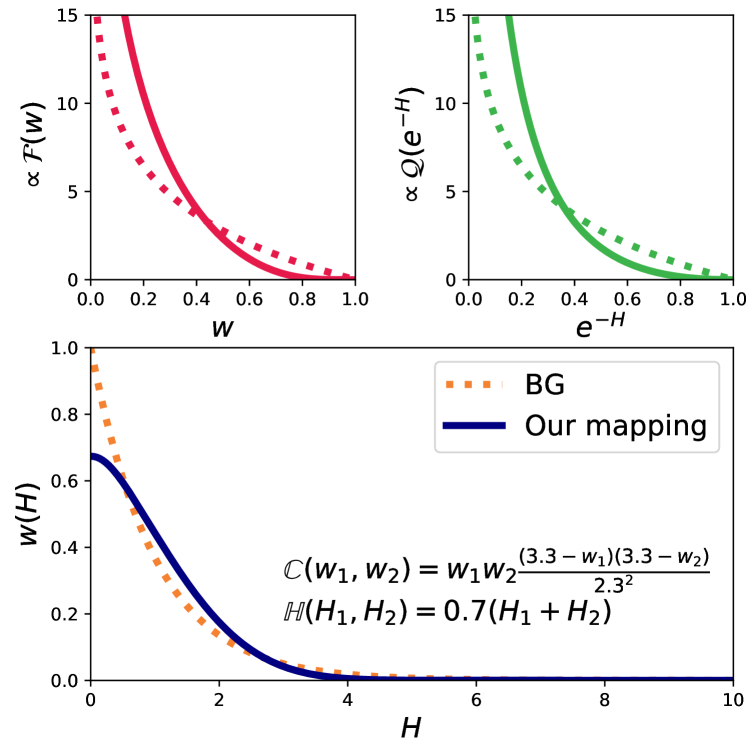
Figure 1: The top two panels show the mapping functions $\mathcal{F}$ and $\mathcal{Q}$ for $\bar{w}$ and $q=e^{-H}$, respectively (solid lines), and their BG equivalents (dotted lines). The bottom panel shows the distribution $w(H)=\mathcal{F}^{-1}(\beta(\mathcal{H}(H)-H_{o}))$ (solid line) for the mappings in Eqs. (14) and (15), and the normalized BG distribution with the same average energy (dotted line).

VII Conclusions

We employed an approach based on Liouville’s theorem for equilibrium conditions obeying a thermodynamic limit and self-similarity criterion, to provide an alternative derivation of consistent generalized thermostatistics for systems with correlations and nonadditive Hamiltonians (this is in comparison to the conventional MaxEnt formulations Jaynes (1957a, b); Naudts (2011); Tsallis (2009)). In our formalism, the equilibrium distributions of such systems are fully characterized by $\mathcal{G}$ in Eq. (3) or by $\{\mathcal{F},\mathcal{H}\}$ maps in Eq. (9) for the special cases. Upon appropriate choices of $\{\mathcal{F},\mathcal{H}\}$, our generalized thermostatistic class recovers well-established families, i.e. the standard Jaynes and Tsallis $q$-thermostatistics as demonstrated in Table 1. Interestingly, our formalism implies that, for systems satisfying our criteria, the latter family of thermostatistics can only capture the thermodynamics of systems with additive Hamiltonians.

Our extension of the MaxEnt principle with $S^{\text{GS}}$ to include self-similar correlations as priors, gives an independent derivation of the same equilibrium distributions derived using Liouville’s theorem. This independent derivation confirms the central role of the MaxEnt principle applied to $S^{\text{GS}}$ as a basis for statistical inference in thermostatistics Shore and Johnson (1980). Moreover, it also clarifies the controversy surrounding the heuristic application of the MaxEnt principle to generalized entropy functionals, such as the Tsallis entropy. Our derivation of the Tsallis distribution from Liouville’s theorem and the MaxEnt principle applied to $\SS^{\text{GS}}$, with a self-similar correlation prior, provides it with the mathematical support it previously lacked. Moreover, the fact that the Tsallis distribution does not satisfy Shore and Johnson’s independent-system axiom Shore and Johnson (1980); Pressé et al. (2013, 2015); Tsallis (2015) is no longer a problem, because it satisfies our criterion for self-similar correlated systems, which is more general than Shore and Johnson’s system independence.

It would be interesting to examine the thermodynamics of low-dimensional long-range Ising-type models Dauxois2002 ; Latora et al. (2002); Salazar and Toral (1999); Salazar et al. (2000); Portesi et al. (1995); Apostolov2009 ; Thouless1969 ; Dyson1971 ; Ruelle1968 , which exhibit phase transitions under certain conditions Thouless1969 ; Dyson1971 ; Ruelle1968 . In the context of our formalism, such phase transitions are driven by the set of control parameters given above as $\{a^{X},b^{X}\}$ (and which include the temperature through a global function (SaadatmandPrep, )).

In this supplemental material, we first discuss the restrictions on the normalization of Tsallis distribution and when it can be considered as a valid probability. We then present a simple example of finding the distribution function, $\mathcal{G}$, satisfying Eq. (8) of the main text. The proof of Theorem II of the main text and an associated nontrivial example is given in Sec. III. Later, in Sec. IV, we discuss how to find Eq. (13) from Eq. (12). In Sec. V, we demonstrate how our formalism recovers $w^{\rm BG}$ for the trivial case of one-dimensional Ising ferromagnets at vanishing temperatures. The details of our numerical approach to find $\mathcal{F}$ and $\mathcal{H}$ maps in Eq. (9) is presented in the last section.

VIII Restrictions on the normalization of Tsallis distribution

Care needs to be taken with the normalization of the Tsallis distribution, $w_{\mathbf{z}}\propto e_{q}^{\mathfrak{b}H_{\mathbf{z}}}$, that is introduced following Eq. (6) in the main text Lutsko2011 . For example, it cannot be normalized and interpreted as a valid probability distribution when $q>1$, $\mathfrak{b}<0$ and the Hamiltonian involves unbounded kinetic energy terms. It can, however, be normalised for $\mathfrak{b}>0$ for $q>\!2$. Also, it is important to note that $\mathfrak{b}$ is not generally the negative of the inverse temperature and has a nontrivial connection to the physical temperature; a consistent equilibrium $q$-thermostatistics is presented in SaadatmandPrep .

IX Recovering $w^{\rm BG}$ using Equation (8)

In the main text, we argued that finding $\mathcal{G}$ to satisfy Eq. (8) of the main text results in the equilibrium distribution in Eq. (3). Here is a simple example: consider a conventional short-range-interacting system where the relations $w^{AB}=w^{A}w^{B}$ and $H^{AB}=H^{A}+H^{B}$ hold to a very a good approximation. In this case, $\mathbb{C}(w^{A},w^{B})=w^{A}w^{B}$ and $\mathbb{H}(H^{A},H^{B})=H^{A}+H^{B}$. Equation (8) becomes $w^{A}w^{B}=\mathcal{G}(H^{A}+H^{B})$, which is trivially satisfied by any $\mathcal{G}$ satisfying $f_{\mathbf{z}}=\mathcal{G}(a\ln(f_{\mathbf{z}})+b)$ (or equivalently $\mathcal{G}(H_{\mathbf{z}})=e^{-b/a}e^{H_{\mathbf{z}}/a}$); here $f_{\mathbf{z}}$ is a bounded, otherwise arbitrary, phase-space function, $\{a,b\}$ are constants of integration, and we have $b^{AB}=b^{A}+b^{B}$, where $b^{X}$ is proportional to the size of the system $X$ as before. This gives the Boltzmann-Gibbs (BG) exponential class of distributions $w^{\rm BG}_{\mathbf{z}}=e^{-\beta H_{\mathbf{z}}}/Z^{\rm BG}$ with $Z^{\rm BG}=\sum_{z}e^{-\beta H_{z}}=e^{-\beta\bar{H}+k^{-1}S^{\rm GS}}$, as expected. Here, we have $\beta\equiv-1/a$, $b\equiv-\ln(Z^{\rm BG})/\beta=\bar{H}-S^{\rm GS}/(k\beta)$, $S^{\text{GS}}(\{w_{\mathbf{z}}\})=-k\sum_{\mathbf{z}}w_{\mathbf{z}}\ln(w_{\mathbf{z}})$ and, therefore, it is clear that the constants $\beta$, $\bar{H}$, and $Z^{\rm BG}$ can be generally interpreted as the inverse temperature of the equilibrium, internal mean energy, and partition function respectively (as illustrated in Table I of the main text).

X Proof of Theorem II

We prove Theorem II by combining $\mathcal{F}_{X}(\cdot)$ with the function $\mathcal{G}_{X}(\cdot)$ in Eq. (3) to give the composite function $\mathcal{F}_{X}(w^{X}_{\mathbf{z}})=\mathcal{F}\mathcal{G}_{X^{\prime\prime}}(H^{X}_{\mathbf{z}})$ where $\mathcal{F}\mathcal{G}_{X^{\prime\prime}}\equiv\mathcal{F}_{X}\circ\mathcal{G}_{X^{\prime}}$. This allows Eq. (9a), after $\mathbb{C}(w^{A},w^{B})$ is replaced by $w^{AB}$ according to Eq. (7b), to be written as

$$\mathcal{F}\mathcal{G}_{AB}(H^{AB})=\mathcal{F}\mathcal{G}_{A}(H^{A})+\mathcal{F}\mathcal{G}_{B}(H^{B}).$$ (S1)

In comparison Eq. (9b), with $\mathbb{H}(H^{A},H^{B})$ replaced by $H^{AB}$ according to Eq. (7a), is

$$\mathcal{H}_{AB}(H^{AB})=\mathcal{H}_{A}(H^{A})+\mathcal{H}_{B}(H^{B}),$$ (S2)

which suggests that $\mathcal{F}\mathcal{G}_{X}(\cdot)$ and $\mathcal{H}_{X}(\cdot)$ are related functions. Indeed, the equality $\mathcal{F}\mathcal{G}_{X}(H^{X})=\mathcal{H}_{X}(H^{X})$ satisfies Eqs. (S1) and (S2) as does the linear relationship

$$\mathcal{F}\mathcal{G}_{X}(H^{X})=a^{X}\mathcal{H}_{X}(H^{X})+b^{X}$$ (S3)

for constants $a^{X}$ and $b^{X}$ provided we adopt the system composition rules

$$a^{AB}=a^{A}=a^{B},\qquad b^{AB}=b^{A}+b^{B}.$$ (S4)

Applying the inverse function $\mathcal{F}^{-1}$ to both sides of Eq. (S3) and making use of Eq. (3) then yields the desired result, Eq. (10) with Eq. (S4) as condition Eq. (11). $\Box$

While other relationships may hold, the linear relationship in Eq. (S3) and its corresponding equilibrium distribution in Eq. (10) are sufficient for our purposes here.

As an example of the application of Theorem II, consider a nontrivial correlated and interacting system satisfying $w^{AB}=\mathbb{C}(w^{A},w^{B})=w^{A}\otimes_{q}w^{B}$ and $H^{AB}=\mathbb{H}(H^{A},H^{B})=H^{A}\oplus_{p}H^{B}$, where $\otimes_{q}$ and $\oplus_{p}$ are the generalized product and sum of the $q$-algebra respectively Suyari (2006); Tsallis (2009). It is clear that choosing $\mathcal{F}=\ln_{q}$ will result in $\mathcal{F}(\mathbb{C}(w^{A},w^{B}))=\mathcal{F}(w^{A})+\mathcal{F}(w^{B})$, while setting $\mathcal{H}(H_{\mathbf{z}})=\ln(e_{p}^{H_{\mathbf{z}}})$ gives $\mathcal{H}(\mathbb{H}(H^{A},H^{B}))=\mathcal{H}(H^{A})+\mathcal{H}(H^{B})$. Therefore, Eq. (7) tells us that the equilibrium distribution is simply $w_{\mathbf{z}}=\exp_{q}\big{(}a\ln(e_{p}^{H_{\mathbf{z}}})+b\big{)}$. This example appears in Table I in the main text.

XI Finding Equation (13) given Equation (12)

In the main text, we argued that the constrained maximization of $S^{\text{GS}}(\{w^{AB}_{\mathbf{z}}\})/k$ leads to $\frac{\partial}{\partial w^{AB}_{\mathbf{z}_{AB}^{\prime}}}[-\sum_{\mathbf{z}_{AB}}\ln w^{AB}_{\mathbf{z}_{AB}}+aI(\{w^{AB}_{\mathbf{z}_{AB}}\})\!+\!bE(\{w^{AB}_{\mathbf{z}_{AB}}\})+\sum_{\mathbf{z}_{AB}}c_{\mathbf{z}_{AB}}(w^{AB}_{\mathbf{z}_{AB}}-\mathbb{C}(w^{A}_{\mathbf{z}_{A}},w^{B}_{\mathbf{z}_{B}}))]=0$ with Lagrange multipliers $a$, $b$, and $\{c_{\mathbf{z}_{AB}}\}$, where $c_{\mathbf{z}_{AB}}$ is a function over the phase space.

As $\mathbb{C}(w^{A}_{\mathbf{z}_{A}},w^{B}_{\mathbf{z}_{B}})$ has no explicit dependence on $w^{AB}_{\mathbf{z}_{AB}}$, the above equation results in $-\!1\!-\!\ln w^{AB}_{\mathbf{z}_{AB}}\!+\!a\!+\!bH^{AB}_{\mathbf{z}_{AB}}\!+\!c_{\mathbf{z}_{AB}}=0$. From Axiom II, this gives

$$\ln w^{X}_{\mathbf{z}_{X}}=a^{X}+b^{X}H^{X}_{\mathbf{z}_{X}}+c^{X}_{\mathbf{z}_{X}}$$ (S5)

for $X=A$, $B$, and $AB$, where we have redefined $a^{X}$ as $1+a^{X}$ for convenience. Taking Eq. (S5) with $X=AB$, and substituting for $w^{AB}_{\mathbf{z}_{AB}}$ and $H^{AB}_{\mathbf{z}_{AB}}$ using Eq. (6) gives $\ln\mathbb{C}(w^{A}_{\mathbf{z}_{A}},w^{B}_{\mathbf{z}_{B}})=a^{AB}+b^{AB}\mathbb{H}(H^{A}_{\mathbf{z}_{A}},H^{B}_{\mathbf{z}_{B}})+c^{AB}_{\mathbf{z}_{AB}}$. Taking this and substituting for $H^{A}_{\mathbf{z}_{A}}$ and $H^{B}_{\mathbf{z}_{B}}$ using Eq. (S5) with $X=A$ and $B$, respectively, then yields $\frac{1}{b^{AB}}[\ln\mathbb{C}(w^{A}_{\mathbf{z}_{A}},w^{B}_{\mathbf{z}_{B}})\!-\!a^{AB}\!-\!c^{AB}_{\mathbf{z}_{AB}}]=\mathbb{H}(\frac{1}{b^{A}}[\ln w^{A}_{\mathbf{z}_{A}}\!-\!a^{A}\!-\!c^{A}_{\mathbf{z}_{A}}],\frac{1}{b^{B}}[\ln w^{B}_{\mathbf{z}_{B}}\!-\!a^{B}\!-\!c^{B}_{\mathbf{z}_{B}}])$ as required.

XII Recovering $w^{\rm BG}$ for one-dimensional Ising ferromagnets

Consider macroscopic steady-state ground states of the nearest-neighbor Ising model, $H_{\rm Ising}=-J\sum_{i}S_{i}S_{i+1},~{}J>0,~{}S_{i}=\pm 1~{}\forall i$ (e.g. see Baxter (2007) for a review). It can be easily shown that this system is describable, with a good approximation, by $w^{AB}_{(\mathfrak{i},\mathfrak{j})}=\mathbb{C}(w^{A}_{\mathfrak{i}},w^{B}_{\mathfrak{j}})=w^{A}_{\mathfrak{i}}w^{B}_{\mathfrak{j}}\exp[-\gamma(1-|m^{AB}_{(\mathfrak{i},\mathfrak{j})}|)]$ and $H^{AB}_{(\mathfrak{i},\mathfrak{j})}=\mathbb{H}(H^{A}_{\mathfrak{i}},H^{B}_{\mathfrak{j}})=H^{A}_{\mathfrak{i}}+H^{B}_{\mathfrak{j}}$ (neglecting the interaction term and boundary effects due to the large size of the systems) — here, $\mathfrak{i}$ denotes a collective spin state, $\gamma\rightarrow\infty$ (playing the role of the diverging inverse temperature and, therefore, the exponential acts effectively as a $\delta_{m^{A}_{\mathfrak{i}},m^{B}_{\mathfrak{j}}}$-function). Also, we use $m^{X}=\sum_{i}S_{i}/N^{X}$, where $N^{X}$ is the number of sites, to denote the magnetization per site for systems $X=A$, $B$, and their composition $AB$. (Notice that the self-similarity rules already imply that, for all single systems, there are two highly likely, equiprobable, and degenerate states with $m_{X}=\pm 1$, as expected from the spontaneous magnetization.) Similar to our previous BG-type example in Sec. I above, it is easy to check $H_{\mathfrak{i}}=\mathcal{G}(a\ln(H_{\mathfrak{i}})+\gamma(1-|m_{\mathfrak{i}}|)+b)$ satisfies Eq. (8) for some constant $a$ and additive parameter $b$ (the middle term in $\mathcal{G}$ argument always vanishes for single systems); therefore, the equilibrium distribution is of the $w^{\rm BG}$-form as expected.

XIII Detailed description of the numerical procedure

Here, we detail the numerical procedure used to calculate $\mathcal{F}$ and $\mathcal{H}$ for arbitrary mappings $\mathbb{C}$ and $\mathbb{H}$. These procedures were used to generate Fig. (1) in the main text.

Of relevance here are three primary points: 1) that $\mathcal{F}$ can be found accurately in most cases; 2) that $\mathcal{H}$ can be found similarly by transforming to $q=e^{-H}$, to get $\mathbb{Q}(q^{A},q^{B})=e^{-\mathbb{H}(-\log(q^{A}),-\log(q^{B}))}$, $\mathcal{H}(H)=\mathcal{Q}(e^{-H})$, and $\mathcal{H}^{-1}=-\log(\mathcal{Q}^{-1})$; 3) that for the BG case, we have $\mathcal{F}^{\text{BG}}\propto-\log(w)$, $\mathcal{Q}^{\text{BG}}\propto-\log(w)$ and $\mathcal{G}^{\text{BG}}=e^{-H}$ in dimensionless units with $\beta^{\text{BG}}=1$.

XIII.1 Finding $\mathcal{F}$ and $\mathcal{F}^{-1}$ given $\mathbb{C}$

To calculate $\mathcal{F}$, we use an iterative procedure over the mapping $\mathbb{C}$. Specifically, we exploit the fact that the mapping $\mathbb{C}(w^{A},w^{B})$ has attractors for $w^{A/B}=0$, and a non-attractive fixed point $w^{A}=w^{B}=1$, and that these are the only fixed points in $[0,1]^{2}$).

Thus, we can use the following procedure:

1. Choose an initial weight value $w_{0}=0.99<1$, and set $\mathcal{F}(w_{0})=f_{0}=0.01$.

2. Choose a secondary value $w_{1}=\mathbb{C}(w_{0},w_{0})$, so that $\mathcal{F}(w_{1})=\mathcal{F}(w_{0})+\mathcal{F}(w_{0})=2f_{0}$.

3. Iterate $w_{n>1}=\mathbb{C}(w_{n-1},w_{n})$ until $w_{n}<1E-5$, and evaluate $\mathcal{F}(w_{n>1})=\mathcal{F}(w_{n-1})+\mathcal{F}(w_{n-2})$ using existing values.

This gives a set of pairs of values $(w_{i},\mathcal{F}(w_{i}))$ over $i$, where we got $O(10)$ pairs in all our tests.

Our next step is to generate a continuous function $\mathcal{F}(w)$. We recognize that, for the BG mapping $\mathbb{C}_{\text{BG}}(w^{A},w^{B})=w^{A}w^{B}$, we get $\mathcal{F}_{\text{BG}}(w)\propto-\log(w)$. Running the BG case through the distribution gives $w_{i}=w_{0}^{i}$, and $\mathcal{F}(w_{i})=(i+1)f_{0}$. Clearly, this gives evenly distributed pairs $(\log(w_{i}),\mathcal{F}(w_{i}))$.

We assume that this behaviour is approximately preserved in general mappings. We thus evaluate $\mathcal{F}(w)$ for general $w$ by interpolating (using a cubic spline) the pairs we obtained by iteration on the logarithm of the weights, i.e., we interpolate $\mathcal{F}(w_{n})$ versus $\log(w_{n})$. This method is exact for the BG case. Without loss of generality, we finally normalize $\mathcal{F}$ so that $\int_{0}^{1}x\mathcal{F}(x)dx=1$.

As a final step, we recognise that $\mathcal{F}$ is monotone. This means we can similarly find the inverse function $\mathcal{F}^{-1}(z)$ by interpolating $\log(x_{n})$ versus $\mathcal{F}(x_{n})$, which is again exact for the BG case.

XIII.2 Finding $\mathcal{H}$ and $\mathcal{H}^{-1}$ given $\mathbb{H}$

We note that this iterative approach does not work for $\mathbb{H}$, which does not have any fixed point. But it does work for $q=e^{-H}$, giving

$$\mathbb{Q}(q^{A},q^{B})= e^{-\mathbb{H}(-\log(q^{A}),-\log(q^{B}))},$$ (S6)

with $\mathcal{H}(H)=\mathcal{Q}(e^{-H})$ and $\mathcal{H}^{-1}=-\log(\mathcal{Q}^{-1})$. We can thus use the above approach to calculate mappings for $\mathbb{H}$, by going via $\mathbb{Q}$. Note that in the BG case, we find $\mathcal{Q}_{\text{BG}}(q)\propto-\log(q)$ and see that the method is once again exact.

References

- (1) J. F. Lutsko, J. P. Boon, EPL 95, 20006 (2011).
- (2) F. Tanjia, S. N. Saadatmand, and J. A. Vaccaro, In Preparation .
- Suyari (2006) H. Suyari, Physica A: Statistical Mechanics and its Applications 368, 63 (2006).
- Tsallis (2009) C. Tsallis, Introduction to Nonextensive Statistical Mechanics (Springer, 2009).
- Baxter (2007) R. Baxter, Exactly Solved Models in Statistical Mechanics, Dover books on physics (Dover Publications, 2007).