Unbiased Estimation of the Reciprocal Mean for Non-negative Random Variables

Abstract

Many simulation problems require the estimation of a ratio of two expectations. In recent years Monte Carlo estimators have been proposed that can estimate such ratios without bias. We investigate the theoretical properties of such estimators for the estimation of $\beta=1/\mathbb{E}\,Z$, where $Z\geq 0$. The estimator, $\widehat{\beta}(w)$, is of the form $w/f_{w}(N)\prod_{i=1}^{N}(1-w\,Z_{i})$, where $w<2\beta$ and $N$ is any random variable with probability mass function $f_{w}$ on the positive integers. For a fixed $w$, the optimal choice for $f_{w}$ is well understood, but less so the choice of $w$. We study the properties of $\widehat{\beta}(w)$ as a function of $w$ and show that its expected time variance product decreases as $w$ decreases, even though the cost of constructing the estimator increases with $w$. We also show that the estimator is asymptotically equivalent to the maximum likelihood (biased) ratio estimator and establish practical confidence intervals.

1 Introduction

Over the past few years, unbiased Monte Carlo estimation methods have received significant attention, due to both theoretical interest and practical applications; see, for example, Rhee and Glynn, (2015); Blanchet et al., (2015); Blanchet and Glynn, (2015); Jacob and Thiery, (2015); McLeish, (2011). Efficient unbiased estimation of non-linear functions of expectations of random variables is challenging and has several applications; see, for example, Blanchet et al., (2015); Jacob and Thiery, (2015). An important “canonical” case is the unbiased estimation of $1/\mathbb{E}\,Z$ for a non-negative random variable $Z$. Applications include regenerative simulation, estimating parameters involving densities with unknown normalizing constants, and Bayesian inference.

Motivated by these applications, we study properties of an unbiased estimator of $\beta=1/\mathbb{E}\,Z$ proposed by Blanchet et al., (2015) (which is in turn based on the ideas proposed by Rhee and Glynn, (2015) in the context of stochastic differential equations). The estimator is obtained as follows. Write $\beta=\frac{1}{\mathbb{E}\,Z}=w\,\sum_{n=0}^{\infty}(1-w\,\mathbb{E}\,Z)^{n}$ for $w<2\beta$; here the condition $w<2\beta$ guarantees the convergence of the geometric series $\sum_{n=0}^{\infty}(1-w\,\mathbb{E}\,Z)^{n}$. Further, let $\{Z_{i},i\geq 0\}$ be a sequence of iid copies of $Z$, and let $N$ be a non-negative integer-valued random variable with $q_{n}:=\mathbb{P}(N=n)>0$, for all $n\geq 0$. Then

$$\frac{1}{\mathbb{E}\,Z} =w\sum_{n=0}^{\infty}q_{n}\frac{(1-w\,\mathbb{E}\,Z)^{n}}{q_{n}}=w\sum_{n=0}^{\infty}q_{n}\frac{\mathbb{E}\prod_{i=1}^{n}(1-w\,Z_{i})}{q_{n}}=w\,\mathbb{E}\left[\frac{1}{q_{N}}\prod_{i=1}^{N}(1-w\,Z_{i})\right].$$

Define,

$$\widehat{\beta}(w):=\frac{w}{q_{N}}\prod_{i=1}^{N}(1-w\,Z_{i}).$$ (1)

Clearly, ${\mathbb{E}\widehat{\beta}(w)=\beta}$ and thus $\widehat{\beta}(w)$ is an unbiased estimator of $\beta$. Note that if $Z\leq b$ almost surely for a constant $b$, then with the choice $w<1/b$, $\widehat{\beta}(w)$ becomes non-negative. In this paper, the goal is to study optimal choices for $w$ and ${\{q_{n},n\geq 0\}}$ that make $\widehat{\beta}(w)$ efficient. In particular, a brief description of our contributions is as follows:

• When $\{q_{n},n\geq 0\}$ is the variance-minimizing distribution for a fixed $w$, we show that as $w\searrow 0$, the expected cost to construct $\widehat{\beta}(w)$ increases to $\infty$, while both the variance and the expected time variance product of $\widehat{\beta}(w)$ decease.

• As a consequence, we argue that for any $w$, instead of approximating $\beta$ with a sample mean of iid copies of $\widehat{\beta}(w)$, it is optimal to approximate it by just one outcome of $\widehat{\beta}(w^{*})$, where $w^{*}$ is such that $w^{*}<w$ and the expected cost of constructing $\widehat{\beta}(w^{*})$ is the same as that of the sample mean.

• We study the asymptotic distribution of $\widehat{\beta}(w)$ as $w\searrow 0$ (i.e., as the expected computational cost for the estimator goes to $\infty$). We establish a central limit theorem type convergence result that is useful for finding asymptotically valid confidence intervals.

• We compare the asymptotic performance of the unbiased estimator $\widehat{\beta}(w)$ with that of the maximum likelihood (biased) ratio estimator, where $\beta$ is estimated using the reciprocal of a sample mean of iid copies of $Z$.

• The above results are studied under the assumption that $N$ has the variance-minimizing distribution. Generating samples from this distribution is impossible as it involves unknown parameters. Since $\widehat{\beta}(w)$ is unbiased even for a different distribution of $N$, we develop a method to implement the estimator by proposing a distribution for $N$ (using samples of $Z$) that closely resembles to the variance-minimizing distribution .

Background: Several applications of Monte Carlo simulation involve the estimation of $\beta=1/\mathbb{E}\,Z$ for a non-negative random variable $Z$. In some applications it is a desirable property to have an unbiased estimator of $\beta$ when the magnitudes of the available biased estimators are unknown a priori. Examples include the estimation of a steady-state parameter $\alpha=\mathbb{E}R/\mathbb{E}\tau$ for a regenerative stochastic process, where $\tau$ denotes the length of a regenerative cycle and $R$ denotes the cumulative reward obtained over the regenerative cycle; see, e.g, Glynn, (2006); Asmussen and Glynn, (2007); Moka and Juneja, (2015). It is evident that we have an unbiased estimator of $\alpha$ if we have an unbiased estimator of $1/\mathbb{E}\tau$. A similar case is where parameters can be expressed as $\alpha={\mathbb{E}\left[h(X)f(X)\right]/\mathbb{E}f(X)}$ for some real-valued function $h$ and probability density $f$, where $f$ is known up to the normalizing constant $\mathbb{E}f(X)$. Such densities occur, for example, in Gibbs point processes (Møller and Waagepetersen, (2003)); and a standard method to estimate such parameters is by using Markov Chain Monte Carlo (MCMC) methods, see Asmussen and Glynn, (2007); Rubinstein and Kroese, (2017). However, in many situations it is difficult to bound the bias of the MCMC estimator, as the mixing time of the Markov chain is unknown. An alternative approach is to use a ratio estimator, where $\alpha$ is approximated by ratio of the sample means of the numerator and the denominator. However, this still returns a biased estimator and the bias decreases at a rate that is inversely proportional to the sample size; see Remark 2 and also Asmussen and Glynn, (2007). Therefore, it is desirable to have an unbiased estimator for $1/\mathbb{E}f(X)$ (and equally for $1/\mathbb{E}\tau$) that has the same order of complexity as that of the ratio estimator.

Most importantly, in some applications, having an unbiased estimator of $\beta$ is essential. For example, in the study of doubly intractable models in Bayesian inference, it is assumed that the observations follow a distribution with a density of the form $f(y|\theta)=\frac{g(y,\theta)}{\int g(y,\theta)\mathrm{d}y},$ where $g(y,\theta)$ can be evaluated point-wise up to the normalizing constant $\int g(y,\theta)\mathrm{d}y$; see, for example, Lyne et al., (2015); Walker, (2011); Jacob and Thiery, (2015). Standard Metropolis–Hastings algorithms to obtain posterior estimates are not applicable due to the intractability of the normalizing constant. However, an exact inference method called pseudo-marginal Metropolis–Hastings proposed by Andrieu and Roberts, (2009) can be implemented if a non-negative unbiased estimator of $1/\int g(y,\theta)\mathrm{d}y$ is available; also see Beaumont, (2003); Jacob and Thiery, (2015); Walker, (2011). In particular, Jacob and Thiery, (2015) highlight the importance of the estimators of the form (1).

A standard method called Russian roulette truncation can be used for unbiased estimation of $\beta$. This method is first proposed in the physics literature Carter and Cashwell, (1975); Lux and Koblinger, (1991) and further studied by McLeish, (2011); Glynn and Rhee, (2014); Lyne et al., (2015); Wei and Murray, (2016). The key drawback of these estimators is that they can take negative values with positive probability even when $Z$ is bounded.

Organization of the paper: In Section 2, we study the properties of the estimator as a function of $w$, under the assumption that $N$ has the variance minimizing estimator. An implementable method is proposed in Section 3. A conclusion of the paper is given in Section 4. All the results are proved in Appendix A.

2 Properties of the Estimator

Without loss of generality, assume that $Z$ is non-degenerate. As the estimator $\widehat{\beta}(w)$ in (1) is unbiased, a sample mean of independent copies of $\widehat{\beta}(w)$ is an unbiased estimator of $\beta$ as well. It is well known that the sample mean has square-root convergence rate if $\mathbb{V}\mathrm{ar}\,\widehat{\beta}(w)<\infty$; see, e.g., Asmussen and Glynn, (2007). Thus, a simple strategy is to seek values of $w$ and $\{q_{n},n\geq 0\}$ that minimize $\mathbb{V}\mathrm{ar}\,\widehat{\beta}(w)$. Using the Cauchy–Schwarz inequality, Blanchet et al., (2015) show that for any $w<2\,\mathbb{E}\,Z/\mathbb{E}\,Z^{2}$, $\mathbb{V}\mathrm{ar}\,\widehat{\beta}(w)$ is finite and is minimal if $N$ has a geometric distribution on the non-negative integers with success probability

$$p_{w}=1-\sqrt{\mathbb{E}(1-w\,Z)^{2}}=1-\sqrt{1-2\,w\,\mathbb{E}\,Z+w^{2}\,\mathbb{E}\,Z^{2}};$$

that is, if

$$q_{n}=(1-p_{w})^{n}p_{w},\quad n\geq 0,$$ (2)

where the assumption $w<2\,\mathbb{E}\,Z/\mathbb{E}\,Z^{2}$ guarantees that $p_{w}>0$. Unfortunately, $p_{w}$ depends on $\mathbb{E}\,Z$ and $\mathbb{E}\,Z^{2}$, which are unknown. However, $\widehat{\beta}(w)$ is unbiased even when $N$ has a different distribution. Therefore, in the implementation of $\widehat{\beta}(w)$, we can replace $p_{w}$ with an estimate of $p_{w}$; see Section 3. In this section, we study the properties of $\widehat{\beta}(w)$ under the assumption that $N$ has the distribution (2), because it offers an understanding of what is the best that can be expected from the estimator.

Note that the variance of $\widehat{\beta}(w)$ is given by,

$$\mathbb{V}\mathrm{ar}\,\widehat{\beta}(w) =w^{2}\sum_{n=0}^{\infty}\frac{\left(\mathbb{E}(1-w\,Z)^{2}\right)^{n}}{q_{n}}-\beta^{2}=\frac{w^{2}}{p_{w}^{2}}-\beta^{2},$$ (3)

for all $0<w<2\,\mathbb{E}\,Z/\mathbb{E}\,Z^{2}$. Further, observe that $\mathbb{E}N=1/p_{w}-1$. Now we can ask what is the value of $w\in(0,2\,\mathbb{E}\,Z/\mathbb{E}\,Z^{2})$ that minimizes (3). This question is not addressed in the existing literature. In addition to the variance, it is often important to include the running time to construct the estimator to determine its efficiency; see Glynn and Whitt, (1992). In that case, we need to select $w$ for which the expected time variance product, $\mathbb{E}T\,\mathbb{V}\mathrm{ar}\,\widehat{\beta}(w),$ is minimal, where $T$ is the time required to construct $\widehat{\beta}(w)$. From (1) (since $Z_{1},Z_{2},\dots$ are iid), it is reasonable to assume that $T$ is proportional to the number of $Z_{i}$’s used for constructing $\widehat{\beta}(w)$. Since $N=N(w)$ samples of $Z$ are used in the construction of $\widehat{\beta}(w)$, we assume that the expected time variance product is $\mathbb{E}N\,\mathbb{V}\mathrm{ar}\,\widehat{\beta}(w)$.

Theorem 1.

Suppose that $N$ has the geometric distribution given in (2). Then the following hold true.

• The success probability $p_{w}$ is a strictly concave function of $w\in(0,2\,\mathbb{E}\,Z/\mathbb{E}\,Z^{2})$ with a maximum value of $1-\sqrt{1-(\mathbb{E}\,Z)^{2}/\mathbb{E}\,Z^{2}}$ attained at $w=\mathbb{E}\,Z/\mathbb{E}\,Z^{2}$, and

  $$\lim_{w\searrow 0}p_{w}=\lim_{w\nearrow 2\,\mathbb{E}\,Z/\mathbb{E}\,Z^{2}}p_{w}=0.$$

• The variance $\mathbb{V}\mathrm{ar}\,\widehat{\beta}(w)$ is a strictly increasing convex function of $w\in(0,2\,\mathbb{E}\,Z/\mathbb{E}\,Z^{2})$, with

  $$\lim_{w\searrow 0}\mathbb{V}\mathrm{ar}\,\widehat{\beta}(w)~{}=~{}0\quad\text{ and }\quad\lim_{w\nearrow 2\,\mathbb{E}\,Z/\mathbb{E}\,Z^{2}}\mathbb{V}\mathrm{ar}\,\widehat{\beta}(w)~{}=~{}\infty.$$

• The expected time variance product ${\mathbb{E}N(w)\,\mathbb{V}\mathrm{ar}\,\widehat{\beta}(w)}$ is a strictly increasing function of $w\in(0,2\,\mathbb{E}\,Z/\mathbb{E}\,Z^{2})$, with

  $$\lim_{w\searrow 0}\mathbb{E}N(w)\,\mathbb{V}\mathrm{ar}\,\widehat{\beta}(w)=\frac{\mathbb{V}\mathrm{ar}\,Z}{(\mathbb{E}\,Z)^{4}},\quad\text{ and }\quad\lim_{w\nearrow 2\,\mathbb{E}\,Z/\mathbb{E}\,Z^{2}}\mathbb{E}N(w)\,\mathbb{V}\mathrm{ar}\,\widehat{\beta}(w)=\infty.$$

Remark 1.

To understand the implications of Theorem 1, suppose we select a $w\in\left(0,2\,\mathbb{E}\,Z/\mathbb{E}\,Z^{2}\right)$, giving an expected computational cost of $\mathbb{E}N(w)$ to obtain $\widehat{\beta}(w)$. Further, let $\overline{\beta}_{k}(w)$ be the sample mean of $k$ iid copies of $\widehat{\beta}(w)$. Then the expected time variance product for $\overline{\beta}_{k}(w)$ is

$$k\,\mathbb{E}N(w)\,\mathbb{V}\mathrm{ar}\,\overline{\beta}_{k}(w)=\mathbb{E}N(w)\,\mathbb{V}\mathrm{ar}\,\widehat{\beta}(w).$$

Now suppose that $w^{*}<w$ is selected so that the average cost to generate one outcome of $\widehat{\beta}(w^{*})$ is equal to the average cost to construct $\overline{\beta}_{k}(w)$; that is, $k\,\mathbb{E}N(w)$. Then, from Theorem 1 (iii), for the same computational effort, $\widehat{\beta}(w^{*})$ has a smaller variance than $\overline{\beta}_{k}(w)$ for any feasible $w$ selected as above, and is therefore a better estimator.

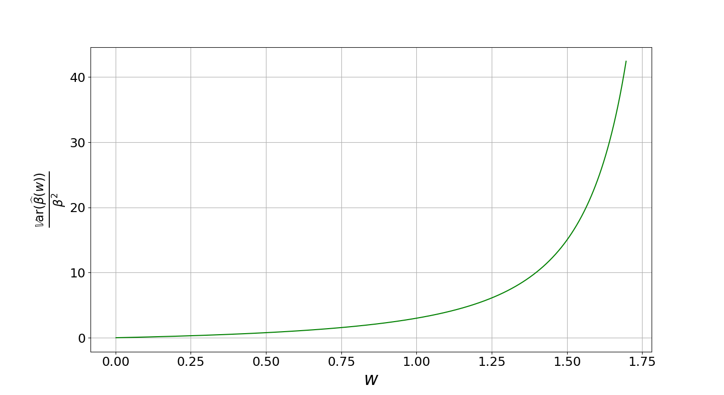
(a)

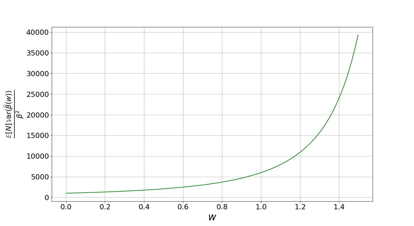
(b)

Figure 1: An example to illustrate the dependency of the performance of the unbiased estimator on parameter $w$. Panels (a) and (b) show, respectively, the relative variance $\frac{\mathbb{V}\mathrm{ar}\,\widehat{\beta}(w)}{\beta^{2}}$ and the expected time relative variance product $\frac{\mathbb{E}N(w)\mathbb{V}\mathrm{ar}\,\widehat{\beta}(w)}{\beta^{2}}$, as functions of $w$.

To illustrate the results of Theorem 1, consider an example where ${Z=\mathbb{I}(A)}$ for an event $A$ with probability ${\mathbb{P}(A)=\mathbb{E}\,Z=0.001}$. Since ${\mathbb{E}\,Z^{2}=0.001}$, the relative variance ${\frac{\mathbb{V}\mathrm{ar}\,Z}{(\mathbb{E}\,Z)^{2}}=999}$. By substituting the values of $\mathbb{E}\,Z$ and $\mathbb{E}\,Z^{2}$, we can calculate $p_{w}$, $\mathbb{E}N$ and $\mathbb{V}\mathrm{ar}\,\widehat{\beta}(w)$ for any ${w<2\,\mathbb{E}\,Z/\mathbb{E}\,Z^{2}=2}$. Figure 1 illustrate the effect of $w$ on the efficacy of the estimator $\widehat{\beta}(w)$. As expected, both $\frac{\mathbb{V}\mathrm{ar}\,\widehat{\beta}(w)}{\beta^{2}}$ and $\frac{\mathbb{E}N(w)\mathbb{V}\mathrm{ar}\,\widehat{\beta}(w)}{\beta^{2}}$ are decreasing as $w\searrow 0$ with the limits $0$ and ${\frac{\mathbb{V}\mathrm{ar}\,Z}{(\mathbb{E}\,Z)^{2}}=999}$, respectively. ∎

Remark 1 motivates us to study the asymptotic distributional properties of $\widehat{\beta}(w)$ as $w\searrow 0$, when $N$ has the geometric distribution given in (2). Theorem 2 is crucial for establishing confidence intervals that are asymptotically valid as $w\searrow 0$.

Theorem 2.

Suppose that $N$ has the distribution given by (2) and $Z$ is bounded. Then, as $w\searrow 0$,

$$(i)\quad\widehat{\beta}(w)\stackrel{{\scriptstyle d}}{{\longrightarrow}}\beta,\quad\quad\text{ and }\quad\quad(ii)\quad\frac{\left(\widehat{\beta}(w)-\beta\right)}{\sqrt{w\,\mathbb{E}\,Z}}\stackrel{{\scriptstyle d}}{{\longrightarrow}}\left(\sqrt{\frac{\mathbb{V}\mathrm{ar}\,Z}{(\mathbb{E}\,Z)^{4}}{\mathcal{E}}(1)}\right){\mathcal{N}}(0,1),$$

where $\stackrel{{\scriptstyle d}}{{\longrightarrow}}$ denotes convergence in distribution, and ${\mathcal{E}}(1)$ and ${\mathcal{N}}(0,1)$ are independent random variables from respectively the standard (mean 1) exponential and standard normal distributions.

We show later in Section A.1 that $\frac{p_{w}}{w\,\mathbb{E}\,Z}\to 1$ as $w\searrow 0$ (see (8)). Since $\mathbb{E}N=1/p_{w}-1$ and $\lim_{w\to 0}p_{w}=0$, $w\,\mathbb{E}Z\>\mathbb{E}N\to 1$ as $w\searrow 0$. That means, an alternative expression for Theorem 2 (ii) is

$$\sqrt{\mathbb{E}N}\left(\widehat{\beta}(w)-\beta\right)\stackrel{{\scriptstyle d}}{{\longrightarrow}}\sigma\sqrt{{\mathcal{E}}(1)}\,{\mathcal{N}}(0,1),\quad\text{ as}\quad w\searrow 0,$$

where $\sigma=\sqrt{\frac{\mathbb{V}\mathrm{ar}\,Z}{(\mathbb{E}\,Z)^{4}}}$. The above expression has more resemblance to the standard central limit theorem, since $\mathbb{E}N$ is the computational cost of the estimator. It is not difficult to show that $\sqrt{{\mathcal{E}}(1)}\,{\mathcal{N}}(0,1)$ is a random variable with density $f(x)=\frac{1}{\sqrt{2}}\exp(-\sqrt{2}|x|)$, which is the density of a mean zero Laplace (or double exponential) distribution with scale $1/\sqrt{2}$. These observations are useful for constructing asymptotically valid confidence intervals as follows. For any given $\alpha\in(0,1)$, by solving $\int_{0}^{t}f(x)\,dx=(1-\alpha)/2$ for $t$, we get $t=-\log(\alpha)/\sqrt{2}$. Then using Theorem 2, we can say that the interval

$$\left(\widehat{\beta}(w)+\frac{\log(\alpha)}{\sqrt{2}}\sigma\sqrt{w\,\mathbb{E}\,Z},\quad\widehat{\beta}(w)-\frac{\log(\alpha)}{\sqrt{2}}\sigma\sqrt{w\,\mathbb{E}\,Z}\right)$$

is an asymptotic $1-\alpha$ confidence interval for $\beta$.

Remark 2 (Comparison with the ratio estimator).

A standard (biased) estimator of $\beta$ is ${1/\bar{Z}_{n}}$, where $\bar{Z}_{n}$ is the sample mean of $n$ iid copies of $Z$. Using Taylor’s theorem for the function $1/x$ about $\mathbb{E}\,Z$, we can easily show that the bias of $1/\bar{Z}_{n}$ is approximately $\frac{1}{n}\frac{\mathbb{V}\mathrm{ar}\,Z}{(\mathbb{E}\,Z)^{3}}$ for large $n$, while, on the other hand, $\widehat{\beta}(w)$ has zero bias. Furthermore, using the same Taylor’s theorem, we can show that the asymptotic time variance product of $1/\bar{Z}_{n}$ is $\mathbb{V}\mathrm{ar}\,Z/(\mathbb{E}\,Z)^{4}$ as $n\to\infty$. From Theorem 1 (iii), the unbiased estimator $\widehat{\beta}(w)$ has the same asymptotic expected time variance product. However, unbiasedness of $\widehat{\beta}(w)$ comes at cost. As an application of the delta method, we can show that the ratio estimator satisfies the central limit theorem: $\sqrt{n}\left(1/\bar{Z}_{n}-\beta\right)\stackrel{{\scriptstyle d}}{{\longrightarrow}}\sqrt{\frac{\mathbb{V}\mathrm{ar}\,Z}{(\mathbb{E}\,Z)^{4}}}\,{\mathcal{N}}(0,1).$ That is, the ratio estimator is asymptotically normal. On the other hand, the asymptotic distribution of the unbiased estimator $\widehat{\beta}(w)$ is Laplace, which has more slowly decaying tails than a normal distribution. In conclusion, the ratio estimator can have narrower confidence intervals than the unbiased estimator.

Remark 3 (Importance sampling).

Just like in the case of the ratio estimator, from Theorems 1 and 2, the relative variance of $Z$ is the key factor influencing the asymptotic properties of the unbiased estimator. The smaller the value is of the relative variance of $Z$, the better is the reliability of the unbiased estimator. One of the most effective technique of variance reduction is importance sampling. We can improve the performance of the estimator if we can implement an importance sampling technique for the random variable $Z$.

Remark 4 (The time variance product minimizing distribution for $N(w)$).

We have assumed that for a given $w$ the random variable $N(w)$ has the variance minimizing distribution given by (2). However, when the criteria for the optimality of $\widehat{\beta}(w)$ is the minimization of the expected time variance product, we need to seek a distribution $\{q_{n},n\geq 0\}$ that minimizes $\mathbb{E}N(w)\mathbb{V}\mathrm{ar}\,\widehat{\beta}(w)$. It is shown in Blanchet et al., (2015) that the distribution that minimizes the expected time variance is given by

$$\widetilde{q}_{n}=\frac{w\,(1-p_{w})^{n}}{\sqrt{\beta^{2}+d_{w}\,n}},n\geq 0,$$ (4)

where $d_{w}$ is the unique (positive) number satisfying $\sum_{n=0}^{\infty}\frac{w\,(1-p_{w})^{n}}{\sqrt{\beta^{2}+d_{w}\,n}}=1.$ When compared to the distribution (2), drawing samples from (4) has an extra difficulty of finding $d_{w}$ by solving an equation that contains an infinite sum. Even if we overcome this difficulty, the reduction in the expected time variance product is typically insignificant, because for small values of $w$,

$$\mathbb{E}\widetilde{N}(w)\,\mathbb{V}\mathrm{ar}\,\widetilde{\beta}(w)=\mathbb{E}N(w)\,\mathbb{V}\mathrm{ar}\,\widehat{\beta}(w)(1+O(w)),$$ (5)

when $N(w)$ has the variance minimizing distribution (2); see Section A.3 for a proof of (5). ∎

3 An Implementation

Recall that the success probability $p_{w}$ of $N$ is a function of unknown quantities $\mathbb{E}\,Z$ and $\mathbb{E}\,Z^{2}$. However, fortunately, $\widehat{\beta}(w)$ in (1) is still an unbiased estimator of $\beta$ for any distribution $\{q_{n},n\geq 0\}$ of $N$. In particular, instead of taking $q_{n}$ as in (2), we can take $q_{n}=P_{k}(1-P_{k})^{n}$, where $P_{k}$ is defined below. Under the proposed implementation, when the given budget is sufficiently large, half of the budget is used for estimating $P_{k}$ and then $w$ is chosen such that the remaining half the budget is used for generating a sample of the unbiased estimator.

To simplify the discussion, assume that there is a known constant $0<\varepsilon\leq\beta$; for example, if $Z\leq b$ for a constant $b$, we can take $\varepsilon=1/b$. Let $\widetilde{Z}_{1},\widetilde{Z}_{2},\dots,\widetilde{Z}_{k}$ be a sequence of iid copies of $Z$, independent of the sequence $Z_{1},Z_{2},\dots$, which is used in the construction of the unbiased estimator $\widehat{\beta}$ in (1). Define the first two sample moments: ${M_{1}(k)=\frac{1}{k}\sum_{i=1}^{k}\widetilde{Z}_{i}}$ and ${M_{2}(k)=\frac{1}{k}\sum_{i=1}^{k}\widetilde{Z}^{2}_{i}}$. If $M_{1}(k)>0$, define,

$$P_{k}=1-\sqrt{\frac{1}{k}\sum_{i=1}^{k}(1-w_{k}\,\widetilde{Z}_{i})^{2}}\quad\text{with}\quad w_{k}=\min\left(\frac{1}{k\,M_{1}(k)},\frac{M_{1}(k)}{M_{2}(k)},\varepsilon\right).$$

Otherwise, take $P_{k}=1/k$ and $w_{k}=\varepsilon/k$. The condition $w_{k}<2\frac{M_{1}(k)}{M_{2}(k)}$ guarantees that $P_{k}>0$. Further, whether $M_{1}(k)=0$ or not, $w_{k}<\beta$ and hence it guarantees that the estmator $\widehat{\beta}(w_{k})$ (defined by (1)) with $q_{n}=P_{k}(1-P_{k})^{n}$ is an unbiased estimator of $\beta$. Note that given $M_{1}(k)$ and $M_{2}(k)$, the expected cost to construct to $\widehat{\beta}(w_{k})$ is $k+1/P_{k}$ (including the cost to construct $P_{k}$), since $\mathbb{E}\left[N(w_{k})\big{|}M_{1}(k),M_{2}(k)\right]=1/P_{k}-1$. Theorem 3 states that for large values of $k$, this total expected cost is approximately $2\,k$, and conditioned on $M_{1}(k)$ and $M_{2}(k)$, the expected time variance product goes to a random variable with mean $4\frac{\mathbb{V}\mathrm{ar}\,Z}{(\mathbb{E}\,Z)^{4}}$. See Section A.4 for a proof Theorem 3.

Theorem 3.

Under the above construction, $\mathbb{E}\widehat{\beta}(w_{k})=\beta$, and as $k\rightarrow\infty$, $k\,P_{k}\to 1,\,a.s.$, and

$$\left(k+\frac{1}{P_{k}}\right)\mathbb{V}\mathrm{ar}\,\left(\widehat{\beta}(w_{k})\big{|}M_{1}(k),M_{2}(k)\right)\longrightarrow 2\frac{\mathbb{V}\mathrm{ar}\,Z}{(\mathbb{E}\,Z)^{4}}\left[1+\chi^{2}_{1}\right],\,a.s.,$$

where $\chi_{1}^{2}$ is the square of a standard normal random variable.

To understand Theorem 3, consider the example given in Remark 1. We estimated the expected total cost $k+\mathbb{E}[1/P_{k}]$ and $\mathbb{V}\mathrm{ar}\,\widehat{\beta}(w_{k})$ using $10000$ samples of $P_{k}$ and $\widehat{\beta}(w_{k})$, respectivley, with $k=10000$. Our simulation results show that the estimated expected time relative variance product is $3969.75$, which is approximately equal to $4\frac{\mathbb{V}\mathrm{ar}\,Z}{(\mathbb{E}\,Z)^{2}}=4\times 999=3996$, as expected.

4 Conclusion

We investigated the theoretical properties of a parametrized family $\{\widehat{\beta}(w),w>0\}$ of unbiased estimators of $1/\mathbb{E}\,Z$ for a non-negative random variable $Z$. We studied the variance and the expected time variance product as functions of $w$ and established several asymptotic results. We showed that with an optimal choice of $w$, the asymptotic performance of the unbiased estimator $\widehat{\beta}(w)$ is comparable to the maximum likelihood (biased) ratio estimator. We further proposed an implementable unbiased estimation based on our results. Similar to Theorem 2, our ongoing research establishes a central limit theorem type convergence result for $\widehat{\beta}(w_{k})$ defined in Section 3, by taking the budget parameter $k\to\infty$.

Appendix A Appendix

To simplify the notation in this section, we use $z_{1}:=\mathbb{E}\,Z$ and $z_{2}:=\mathbb{E}\,Z^{2}$. We also write $p_{w}^{\prime}$ for the derivative $\frac{\mathrm{d}p_{w}}{\mathrm{d}w}$ and $p_{w}^{\prime\prime}$ for the second derivative. ${\mathcal{E}}(\lambda)$ and ${\mathcal{G}}(p)$ denote respectively the mean $1/\lambda$ exponential distribution and the geometric distribution on non-negative integers and the success probability $p$.

A.1 Proof of Theorem 1

From the definition, $p^{\prime}_{w}=(z_{1}-w\,z_{2})/(1-p_{w}).$ It follows that $p^{\prime\prime}_{w}=-\frac{1}{(1-p_{w})^{3}}\left[z_{2}-z_{1}^{2}\right]<0,$ where the strict inequality holds because $z_{2}>z_{1}^{2}$, which follows from the assumption that $Z$ is non-degenerative. Therefore, $p_{w}$ is strictly concave over $(0,2z_{1}/z_{2})$ and it achieves its maximum value $1-\sqrt{1-z_{1}^{2}/z_{2}}$ at $w=z_{1}/z_{2}$. From the definition of $p_{w}$, it is evident that $\lim_{w\searrow 0}p_{w}=\lim_{w\nearrow 2z_{1}/z_{2}}p_{w}=0$.

Recall from (3) that the variance of the estimator is equal to ${w^{2}/p_{w}^{2}}-z_{1}^{2}$. Its derivative can be written as

$$\frac{\mathrm{d}\mathbb{V}\mathrm{ar}\,\widehat{\beta}(w)}{\mathrm{d}w}=2w\,\frac{w\,z_{1}-p_{w}}{p_{w}^{3}(1-p_{w})}$$ (6)

and the second derivative as

$$\frac{\mathrm{d}^{2}\mathbb{V}\mathrm{ar}\,\widehat{\beta}(w)}{\mathrm{d}w^{2}}=\frac{2(w\,z_{1}-p_{w})}{p_{w}^{3}(1-p_{w})^{3}}\left(3\left(w\,z_{1}-p_{w}\right)+2p_{w}\left(p_{w}-w^{2}\,z_{2}\right)\right).$$ (7)

Using Jensen’s inequality, ${\mathbb{E}(1-w\,Z)^{2}>(1-w\,z_{1})^{2}},$ where the strict inequality holds again because $Z$ is non-degenerative. On the other hand, by Bernoulli’s inequality,

$$\sqrt{\mathbb{E}(1-w\,Z)^{2}}=\sqrt{1+(-2w\,z_{1}+w^{2}\,z_{2})}$$

is maximized by $1-w\,z_{1}+w^{2}\,z_{2}/2.$ Thus,

$$z_{1}-w\,z_{2}/2\leq\dfrac{p_{w}}{w}<z_{1}.$$ (8)

Using (8), we have $w\,z_{1}-p_{w}>0$ and $p_{w}-w^{2}\,z_{2}\geq 2wz_{1}-p_{w}>w\,z_{1}$, and hence for all $w\in(0,2z_{1}/z_{2})$, $\frac{\mathrm{d}\mathbb{V}\mathrm{ar}\,\widehat{\beta}(w)}{\mathrm{d}w}>0$ and $\frac{\mathrm{d}^{2}\mathbb{V}\mathrm{ar}\,\widehat{\beta}(w)}{\mathrm{d}w^{2}}>0,$ which establishes the convexity of $\mathbb{V}\mathrm{ar}\,\widehat{\beta}(w)$ over $(0,2z_{1}/z_{2})$.

We now prove that the expected time variance product is a strictly increasing over $(0,2z_{1}/z_{2})$. Let $g_{1}(w):=\mathbb{E}N(w)$, $g_{2}(w):=\frac{\mathbb{V}\mathrm{ar}\,\widehat{\beta}(w)}{\beta^{2}}$ and $g(w):=g_{1}(w)g_{2}(w)=\left(\frac{1}{p_{w}}-1\right)\left(\frac{w^{2}\,z_{1}^{2}}{p_{w}^{2}}-1\right).$ Then,

$$\frac{\mathrm{d}g_{1}}{\mathrm{d}w}(w)=\frac{w\,z_{2}-z_{1}}{p_{w}^{2}(1-p_{w})},\quad\text{ and }\quad\frac{\mathrm{d}g_{2}}{\mathrm{d}w}(w)=2w\,z_{1}^{2}\left[\frac{w\,z_{1}-p_{w}}{p_{w}^{3}(1-p_{w})}\right],$$

and hence, we write

$$\frac{\mathrm{d}g}{\mathrm{d}w}(w) =\frac{2w\,z_{1}^{2}(1-p_{w})(w\,z_{1}-p_{w})+(w^{2}\,z_{1}^{2}-p_{w}^{2})(w\,z_{2}-z_{1})}{p_{w}^{4}(1-p_{w})}$$

$$=\frac{wz_{1}-p_{w}}{p_{w}^{4}(1-p_{w})}\left[w\,p_{w}(z_{2}-z_{1}^{2})+z_{1}(w\,z_{1}-p_{w})+w\,z_{1}(w\,z_{2}-z_{1}p_{w})\right]>0,$$

where the inequality holds because $z_{2}>z_{1}^{2}$, $w\,z_{1}>p_{w}$ and $w\,z_{2}>w\,z_{1}^{2}>z_{1}\,p_{w}$. Therefore, $\mathbb{E}N(w)\,\mathbb{V}\mathrm{ar}\,\widehat{\beta}(w)$ is strictly increasing over $(0,2z_{1}/z_{2})$.

The claims that $\lim_{w\nearrow 2z_{1}/z_{2}}\mathbb{V}\mathrm{ar}\,\widehat{\beta}(w)=\infty$ and $\lim_{w\nearrow 2z_{1}/z_{2}}\mathbb{E}N(w)\mathbb{V}\mathrm{ar}\,\widehat{\beta}(w)=\infty$ hold trivially because $\lim_{w\nearrow 2z_{1}/z_{2}}p_{w}=0$. To complete the proof of the theorem, we can write, by Taylor’s theorem, for any $x\in(0,1)$: $\sqrt{x}=1+\frac{(x-1)}{2}-\frac{(x-1)^{2}}{8}+\frac{(x-1)^{3}}{16\tilde{x}^{5/2}},$ for some $\tilde{x}\in(x,1).$ Consequently,

$$\sqrt{\mathbb{E}(1-w\,Z)^{2}}=1+\frac{\mathbb{E}(1-w\,Z)^{2}-1}{2}-\frac{\left(\mathbb{E}(1-w\,Z)^{2}-1\right)^{2}}{8}+R(w),$$

where $R(w)=\frac{\left(\mathbb{E}(1-w\,Z)^{2}-1\right)^{3}}{16\tilde{x}^{5}/3}$ for some $\tilde{x}\in\left(\mathbb{E}(1-w\,Z)^{2},1\right)$. Since $\tilde{x}\to 1$ as $w\to 0$ and $\mathbb{E}(1-w\,Z)^{2}-1=w^{2}z_{2}-2w\,z_{1}$, we have $R(w)=O(w^{3})$. Further simplification yields that $p_{w}=w\,z_{1}-\frac{w^{2}}{2}\left(z_{2}-z_{1}^{2}\right)+O(w^{3}),$ and thus, $\frac{p^{2}_{w}}{w^{2}\,z^{2}_{1}}=1-\frac{w}{z_{1}}\left(z_{2}-z_{1}^{2}\right)+O(w^{2}).$ Since $1-p_{w}=1+O(w)$,

$$\frac{1-p_{w}}{p_{w}}=\frac{1}{wz_{1}}\left(1+O(w)\right),\quad\text{ and }\quad\frac{w^{2}z_{1}^{2}}{p^{2}_{w}}-1=w\frac{(z_{2}-z_{1}^{2})}{z_{1}}\left(1+O(w)\right).$$ (9)

We conclude that both $\mathbb{V}\mathrm{ar}\,\widehat{\beta}(w)$ and $\mathbb{E}N(w)\mathbb{V}\mathrm{ar}\,\widehat{\beta}(w)$ go to their respective minima as $w\searrow 0$.

A.2 Proof of Theorem 2

Statement (i) follows directly from Theorem 1 and Chebyshev’s inequality:

$$\mathbb{P}\left(|\widehat{\beta}(w)-\beta|>\epsilon\right)\leq\mathbb{V}\mathrm{ar}\,\widehat{\beta}(w)/\epsilon^{2}\to 0,\,\text{ as }\,w\searrow 0,$$

for every $\epsilon>0$. To prove (ii), consider a decreasing sequence ${w_{1}>w_{2}>\cdots}$ such that $w_{1}\leq z_{1}/z_{2}$ and $\lim_{k\to\infty}w_{k}=0$. We construct an almost surely increasing sequence $N_{1}\leq N_{2}\leq\cdots$ such that $N_{k}\sim{\mathcal{G}}(p_{w_{k}})$ and

$$\lim_{k\to\infty}[w_{k}N_{k}]=X_{\infty}/z_{1},\quad a.s.,$$ (10)

for a random variable $X_{\infty}\sim{\mathcal{E}}(1)$. To do so we invoke Theorem 3.1 of Moka and Juneja, (2015). Let $\lambda_{k}=-\log(1-p_{w_{k}})$ and $E_{k}\sim{\mathcal{E}}(\lambda_{k})$. Then, Moka and Juneja, (2015) says that for each $k$, there exist a random variable $Y_{k}$ with cumulative distribution function

$$G_{k}(x)=1-\left(1-\frac{\lambda_{k+1}}{\lambda_{k}}\right)\exp(-\lambda_{k+1}x),\quad x\geq 0,$$

such that $Y_{k}$ is independent of $E_{k}$, and $E_{k+1}$ has the same distribution as $E_{k}+Y_{k}$. Therefore, without loss of generality we assume that there is sequence of independent random variables $Y_{k}\sim G_{k}(x)$ such that $E_{k+1}=E_{k}+Y_{k}=E_{1}+\sum_{i=1}^{k}Y_{i}$ for all $k\geq 1$.

Consider the natural filtration $\left\{\mathscr{F}_{k}=\sigma(E_{1},\dots,E_{k}),k\geq 0\right\}$. Since $E_{k+1}=E_{k}+Y_{k}$,

$$\lambda_{k+1}E_{k+1}-1 =\lambda_{k+1}[E_{k}+Y_{k}-1/\lambda_{k}-\mathbb{E}Y_{k}]=\frac{\lambda_{k+1}}{\lambda_{k}}\lambda_{k}[E_{k}-1/\lambda_{k}]+\lambda_{k+1}[Y_{k}-\mathbb{E}Y_{k}]$$

$$\leq\lambda_{k}E_{k}-1+\lambda_{k+1}[Y_{k}-\mathbb{E}Y_{k}],$$

where the last inequality holds because $\lambda_{k+1}\leq\lambda_{k}$. We have $\mathbb{E}\left[\lambda_{k+1}E_{k+1}|\mathscr{F}_{k}\right]\leq\lambda_{k}E_{k}$ since $Y_{k}$ is independent of $\mathscr{F}_{k}$. Thus, $\displaystyle\left\{X_{k}:=\lambda_{k}E_{k},k\geq 1\right\}$ is a supermartingale (with respect to $\left\{\mathscr{F}_{k}\right\}$). In fact the sequence $\left\{X_{k},k\geq 1\right\}$ is bounded in $\mathcal{L}^{2}$, because $\sup_{k\geq 1}\mathbb{E}X_{k}^{2}=2$, making it uniformly integrable submartingale. Thus, ${X_{\infty}=\lim_{k\to\infty}X_{k}}$ exists $a.s.$ (see Theorem 2 in Section 4 of Chapter VII of Shiryaev, (1996)). Since $\mathbb{P}\left(X_{k}\leq x\right)=\mathbb{P}\left(E_{k}\leq\frac{x}{\lambda_{k}}\right)=1-\exp\left(-x\right).$ This implies that $X_{\infty}\sim{\mathcal{E}}(1)$.

Let $N_{k}=\lfloor E_{k}\rfloor$. Then for all $k$ we have $N_{k}\sim{\mathcal{G}}(p_{w_{k}})$ and $N_{k}\leq N_{k+1}$. From (8), $\lim_{k\to\infty}(1-p_{w_{k}})^{1/w_{k}}=\exp(-z_{1})$ and hence $\lim_{k\to\infty}\frac{w_{k}}{\lambda_{k}}=1/z_{1}$. From the convergence of the sequence $X_{1},X_{2},\dots$, we have $\frac{w_{k}}{\lambda_{k}}X_{k}-w_{k}\leq w_{k}N_{k}\leq\frac{w_{k}}{\lambda_{k}}X_{k}$. Therefore, (10) holds.

Now define

$$\widehat{\beta}_{k}:=\frac{w_{k}}{(1-p_{w_{k}})^{N_{k}}p_{w_{k}}}\prod_{i=1}^{N_{k}}(1-w_{k}Z_{i}).$$ (11)

From the definitions, $\widehat{\beta}_{k}$ is identical to $\widehat{\beta}(w_{k})$ in distribution. We now conclude the proof Theorem 2 by establishing lower and upper bounds on $\widehat{\beta}_{k}$ separately. Let $b$ be an upper bound on $Z$. From the construction of $\widehat{\beta}_{k}$ given by (11), for all $k$ such that $w_{k}<1/b$, we have using (8) that

$$\widehat{\beta}_{k} \geq\frac{1}{z_{1}(1-p_{w_{k}})^{N_{k}}}\exp\left(\sum_{i=1}^{N_{k}}\log(1-w_{k}Z_{i})\right)\geq\frac{1}{z_{1}}\exp\left(N_{k}w_{k}(z_{1}-w_{k}z_{2}/2)+\sum_{i=1}^{N_{k}}\log(1-w_{k}Z_{i})\right).$$

Using Taylor’s theorem, $\log(1-x)\geq-x-\frac{x^{2}}{2(1-x)^{2}}$ for any $x\geq 0$, and thus,

$$\widehat{\beta}_{k} \geq\frac{1}{z_{1}}\exp\left(N_{k}w_{k}z_{1}-N\frac{w_{k}^{2}z_{2}}{2}-w_{k}\sum_{i=1}^{N_{k}}Z_{i}-\sum_{i=1}^{N_{k}}\frac{w_{k}^{2}Z^{2}_{i}}{2(1-w_{k}Z_{i})^{2}}\right)$$

$$=\frac{1}{z_{1}}\exp\left(-N_{k}w_{k}\frac{1}{N_{k}}\sum_{i=1}^{N_{k}}(Z_{i}-z_{1})-\frac{N_{k}w_{k}^{2}}{2}\left(z_{2}+\frac{b^{2}}{(1-w_{k}b)^{2}}\right)\right).$$ (12)

On the other hand, from (11) and (8),

$$\widehat{\beta}_{k} \leq\frac{w_{k}}{(1-p_{w_{k}})^{N_{k}}p_{w_{k}}}\exp\left(-\sum_{i=1}^{N_{k}}w_{k}Z_{i}\right)\leq\frac{w_{k}}{(1-w_{k}z_{1})^{N_{k}}p_{w_{k}}}\exp\left(-\sum_{i=1}^{N_{k}}w_{k}Z_{i}\right)$$

$$=\frac{w_{k}}{p_{w_{k}}}\exp\left(-\sum_{i=1}^{N_{k}}w_{k}Z_{i}-N_{k}\log(1-w_{k}z_{1})\right)$$

$$=\frac{w_{k}}{p_{w_{k}}}\exp\left(-w_{k}N_{k}\frac{1}{N_{k}}\sum_{i=1}^{N_{k}}(Z_{i}-z_{1})+N_{k}w^{2}_{k}\frac{z_{1}^{2}}{2(1-w_{k}z_{1})^{2}}\right).$$ (13)

Using the strong law of large numbers and Theorem 1 of Richter, (1965),

$$\lim_{k\to\infty}\frac{1}{N_{k}}\sum_{i=1}^{N_{k}}(Z_{i}-z_{1})=0,\,a.s.$$

Further, using (8) and (10), we have that $\lim_{k\to\infty}\widehat{\beta}_{k}=\beta$ almost surely. From Taylor’s theorem with a Cauchy remainder term, we have almost surely

$$\log(\widehat{\beta}_{k})-\log(\beta) =\frac{(\widehat{\beta}_{k}-\beta)}{\beta}-\frac{(\widehat{\beta}_{k}-\widehat{X})(\widehat{\beta}_{k}-\beta)}{\widehat{X}^{2}}=\frac{(\widehat{\beta}_{k}-\beta)}{\beta}\left[1+o(1)\right]$$

for a random variable $\widehat{X}$ that takes values between $\widehat{\beta}_{k}$ and $\beta$. Therefore, to complete the proof of (ii), it is enough to show that $\frac{1}{\sqrt{w_{k}}}\log\widehat{\beta}_{k}\stackrel{{\scriptstyle d}}{{\longrightarrow}}\left(\sqrt{\mathbb{V}\mathrm{ar}\,Z\,X_{\infty}}\right){\mathcal{N}}(0,1).$ From (12),

$$\frac{1}{\sqrt{w_{k}}}\log[z_{1}\widehat{\beta}_{k}]\geq-\sqrt{w_{k}N_{k}}\frac{1}{\sqrt{N_{k}}}\sum_{i=1}^{N_{k}}(Z_{i}-z_{1})-\frac{N_{k}w_{k}^{3/2}}{2}\left(z_{2}+\frac{b^{2}}{(1-w_{k}b)^{2}}\right).$$ (14)

From (10) and because $w_{k}\searrow 0$, the second term on the right hand side of the expression goes to zero. Again using (10), we conclude that the right hand side of (14) goes to $\left(\sqrt{\frac{\mathbb{V}\mathrm{ar}\,Z}{z_{1}}X_{\infty}}\right){\mathcal{N}}(0,1)$ in distribution. From (13),

$$\frac{1}{\sqrt{w_{k}}}\log[z_{1}\widehat{\beta}_{k}]\leq\frac{1}{\sqrt{w_{k}}}\log\left[\frac{z_{1}w_{k}}{p_{w_{k}}}\right]-\sqrt{w_{k}N_{k}}\frac{1}{\sqrt{N_{k}}}\sum_{i=1}^{N_{k}}(Z_{i}-z_{1})+N_{k}w_{k}^{3/2}\frac{z_{1}^{2}}{2(1-w_{k}z_{1})^{2}}.$$

We complete the proof because from (8), as $k\to\infty$,

$$0\leq\frac{1}{\sqrt{w_{k}}}\log\left[\frac{z_{1}w_{k}}{p_{w_{k}}}\right]\leq\frac{1}{\sqrt{w_{k}}}\log\left[\frac{1}{\left(1-\frac{w_{k}z_{2}}{2z_{1}}\right)}\right]=-\sqrt{w_{k}}\log\left[\left(1-\frac{w_{k}z_{2}}{2z_{1}}\right)^{1/w_{k}}\right]\to 0,\quad a.s.$$

A.3 Proof of (5)

First, observe from the definitions that $\mathbb{E}\widetilde{N}(w)\mathbb{V}\mathrm{ar}\,\widetilde{\beta}(w)\leq\mathbb{E}N(w)\mathbb{V}\mathrm{ar}\,\widehat{\beta}(w).$ Further using the fact that $\beta=1/z_{1}$ and (8),

$$\mathbb{E}\widetilde{N}(w) \geq\sum_{n=1}^{\infty}n\frac{p_{w}(1-p_{w})^{n}}{\sqrt{1+d_{w}m^{2}_{1}n}}$$

$$=\mathbb{E}N(w)\sum_{n=1}^{\infty}\frac{1}{\sqrt{1+d_{w}z_{1}^{2}n}}\frac{np_{w}(1-p_{w})^{n}}{\mathbb{E}N(w)}$$

$$\geq\mathbb{E}N(w)\frac{1}{\sqrt{1+d_{w}z_{1}^{2}\mathbb{E}N(w)^{2}/\mathbb{E}N(w)}},$$

where the last inequality holds from Jensen’s inequality, because $1/\sqrt{1+ax}$ is a convex function of $x$ for any constant $a>0$ and $\left(\frac{np_{w}(1-p_{w})^{n}}{\mathbb{E}N(w)},n\geq 0\right)$ is a probability distribution. Furthermore, using $\mathbb{E}N(w)^{2}=\mathbb{E}N(w)\frac{(2-p_{w})}{p_{w}}\leq 2\,\mathbb{E}N(w)/p_{w}$, we write $\mathbb{E}\widetilde{N}(w)\geq\mathbb{E}N(w)\frac{1}{\sqrt{1+2d_{w}z_{1}^{2}/p_{w}}}.$ Since the distribution (4) is not the variance minimizing distribution, we have

$$\mathbb{E}\widetilde{N}(w)\mathbb{V}\mathrm{ar}\,\widetilde{\beta}(w) \geq\mathbb{E}\widetilde{N}(w)\mathbb{V}\mathrm{ar}\,\widehat{\beta}(w)\geq\mathbb{E}N(w)\mathbb{V}\mathrm{ar}\,\widehat{\beta}(w)\left(\frac{1}{\sqrt{1+2d_{w}z_{1}^{2}/p_{w}}}\right).$$

We establish (5) by showing that $\frac{1}{\sqrt{1+2d_{w}z_{1}^{2}/p_{w}}}=1+O(w)$. From the definition of $d_{w}$,

$$\frac{wz_{1}}{p_{w}}\sum_{n=0}^{\infty}\frac{p_{w}(1-p_{w})^{n}}{\sqrt{1+d_{w}z_{1}^{2}\,n}}=1,$$

and thus, using $p_{w}\leq wz_{1}$, we write that $1-w\,z_{1}\leq(1-p_{w})\sum_{n=1}^{\infty}\frac{p_{w}(1-p_{w})^{n-1}}{\sqrt{1+d_{w}\,z_{1}^{2}\,n}}\leq(1-p_{w})\frac{1}{\sqrt{1+d_{w}\,z_{1}^{2}}}.$ Consequently, $1+d_{w}\,z_{1}^{2}\leq\left(\frac{1-p_{w}}{1-w\,z_{1}}\right)^{2}$. Hence, using (8), $1+d_{w}\,z_{1}^{2}=1+O(w^{2})$, that is, $d_{w}=O(w^{2})$ and thus, $d_{w}/p_{w}=O(w)$ because $p_{w}=O(w)$. This concludes that $\frac{1}{\sqrt{1+2d_{w}z_{1}^{2}/p_{w}}}=1+O(w)$ and hence establishes (5).

A.4 Proof of Theorem 3

From the assumption, we have $w_{k}\leq\frac{M_{1}(k)}{M_{2}(k)}$. Therefore, similar to (8), we can obtain that

$$0<w_{k}\,M_{1}(k)-w_{k}^{2}\,M_{2}(k)/2\leq P_{k}\leq w_{k}\,M_{1}(k).$$ (15)

From the definitions of $w_{k},M_{1}(k)$ and $M_{2}(k)$, it is easy to see that $\lim_{k\to\infty}kw_{k}\,M_{1}(k)=1,\,a.s.$. Using the upper bound in (15), we show that $\delta_{k}:=1-\frac{1+w^{2}_{k}\,z_{2}-2w_{k}z_{1}}{1-P_{k}}$ is lower bounded by $\frac{w_{k}}{1-P_{k}}\left(2z_{1}-M_{1}(k)-w_{k}\,z_{2}\right)$. Since $\lim_{k\to\infty}M_{1}(k)=z_{1},\,a.s.$ and $\lim_{k\to\infty}kw_{k}=1/z_{1},\,a.s.$, for every realization of $\widetilde{Z}_{1},\widetilde{Z}_{2},\dots$, there exists a $K$ such that $\delta_{k}>0$ for all $k\geq K$, and hence $\mathbb{V}\mathrm{ar}\,\left(\widehat{\beta}(w_{k})\big{|}M_{1}(k),M_{2}(k)\right)$ is finite and equal to $\frac{w_{k}^{2}}{P_{k}\delta_{k}}-\beta^{2}$. It is now enough to show that

$$k\,\left(\frac{w_{k}^{2}\,z_{1}^{2}}{P_{k}\delta_{k}}-1\right)\longrightarrow\frac{\mathbb{V}\mathrm{ar}\,Z}{z_{1}^{2}}\left[1+\chi^{2}_{1}\right],\,a.s.,\quad\text{as }k\to\infty.$$

Write $\displaystyle\left(\frac{w_{k}^{2}\,z_{1}^{2}}{P_{k}\delta_{k}}-1\right)=\left(\frac{w_{k}^{2}\,z_{1}^{2}}{p^{2}_{w_{k}}}-1\right)+w_{k}^{2}\,z_{1}^{2}\left(\frac{1}{P_{k}\delta_{k}}-\frac{1}{p^{2}_{w_{k}}}\right)$, where $p_{w_{k}}=1-\sqrt{1+w^{2}_{k}\,z_{2}-2w_{k}\,z_{1}}$. Using (9) and $\lim_{k\to\infty}k\,w_{k}=1/z_{1}$, we have $\lim_{k\to\infty}k\left(\frac{w_{k}^{2}\,z_{1}^{2}}{p^{2}_{w_{k}}}-1\right)=\frac{\mathbb{V}\mathrm{ar}\,Z}{z_{1}^{2}},\,a.s$. By simplifying the terms in $P_{k}\delta_{k}-p^{2}_{w_{k}}$, we have $\frac{1}{P_{k}\delta_{k}}-\frac{1}{p^{2}_{w_{k}}}=\frac{1}{P_{k}\delta_{k}(1-P_{k})}\left(\frac{P_{k}-p_{w_{k}}}{p_{w_{k}}}\right)^{2}.$ Since $P_{k}-p_{w_{k}}=w_{k}\,(M_{1}(k)-z_{1})(1+O(w_{k}))$, we can write $\frac{P_{k}-p_{w_{k}}}{p_{w_{k}}}=\frac{w_{k}}{p_{w_{k}}}(M_{1}(k)-z_{1})(1+O(w))$. Therefore, using $\lim_{k\to\infty}\frac{w_{k}^{2}\,z_{1}^{2}}{P_{k}\delta_{k}(1-P_{k})}=1,\,a.s.$ and the fact that asymptotically $\sqrt{k}(M_{1}(k)-z_{1})$ has a zero-mean normal distribution with variance $\mathbb{V}\mathrm{ar}\,Z$, we complete the proof with the observation that $w_{k}/p_{w_{k}}\to 1/z_{1}$ as $k\to\infty$.

References

- Andrieu and Roberts, (2009) Andrieu, C. and Roberts, G. O. (2009). The pseudo-marginal approach for efficient Monte Carlo computations. Ann. Statist., 37(2):697–725.
- Asmussen and Glynn, (2007) Asmussen, S. and Glynn, P. W. (2007). Stochastic simulation: algorithms and analysis, volume 57 of Stochastic Modelling and Applied Probability. Springer, New York.
- Beaumont, (2003) Beaumont, M. A. (2003). Estimation of population growth or decline in genetically monitored populations. Genetics, 164(3):1139–1160.
- Blanchet et al., (2015) Blanchet, J. H., Chen, N., and Glynn, P. W. (2015). Unbiased Monte Carlo computation of smooth functions of expectations via taylor expansions. In Proceedings of the 2015 Winter Simulation Conference, WSC ’15, pages 360–367, Piscataway, NJ, USA. IEEE Press.
- Blanchet and Glynn, (2015) Blanchet, J. H. and Glynn, P. W. (2015). Unbiased Monte Carlo for optimization and functions of expectations via multi-level randomization. In Proceedings of the 2015 Winter Simulation Conference, WSC ’15, pages 3656–3667, Piscataway, NJ, USA. IEEE Press.
- Carter and Cashwell, (1975) Carter, L. and Cashwell, E. (1975). Particle-transport simulation with the monte carlo method. Technical Report.
- Glynn, (2006) Glynn, P. W. (2006). Chapter 16 simulation algorithms for regenerative processes. In Henderson, S. G. and Nelson, B. L., editors, Simulation, volume 13 of Handbooks in Operations Research and Management Science, pages 477–500. Elsevier.
- Glynn and Rhee, (2014) Glynn, P. W. and Rhee, C.-H. (2014). Exact estimation for markov chain equilibrium expectations. J. Appl. Probab., 51A:377–389.
- Glynn and Whitt, (1992) Glynn, P. W. and Whitt, W. (1992). The asymptotic efficiency of simulation estimators. Operations Research, 40(3):505–520.
- Jacob and Thiery, (2015) Jacob, P. E. and Thiery, A. H. (2015). On nonnegative unbiased estimators. Ann. Statist., 43(2):769–784.
- Lux and Koblinger, (1991) Lux, I. and Koblinger, L. (1991). Monte Carlo particle transport methods : neutron and photon calculations, volume 102. CRC Press. Includes bibliographical references and index.
- Lyne et al., (2015) Lyne, A.-M., Girolami, M., Atchadé, Y., Strathmann, H., and Simpson, D. (2015). On russian roulette estimates for Bayesian inference with doubly-intractable likelihoods. Statist. Sci., 30(4):443–467.
- McLeish, (2011) McLeish, D. (2011). A general method for debiasing a Monte Carlo estimator. Monte Carlo Methods and Applications., 17:301–315.
- Moka and Juneja, (2015) Moka, S. B. and Juneja, S. (2015). Regenerative simulation for queueing networks with exponential or heavier tail arrival distributions. ACM Trans. Model. Comput. Simul., 25(4):22:1–22:22.
- Møller and Waagepetersen, (2003) Møller, J. and Waagepetersen, R. P. (2003). An Introduction to Simulation-Based Inference for Spatial Point Processes, pages 143–198. Springer, New York.
- Rhee and Glynn, (2015) Rhee, C.-H. and Glynn, P. W. (2015). Unbiased estimation with square root convergence for SDE models. Operations Research, 63(5):1026–1043.
- Richter, (1965) Richter, W. (1965). Limit theorems for sequences of random variables with sequences of random indices. Theory of Probability & Its Applications, 10(1):74–84.
- Rubinstein and Kroese, (2017) Rubinstein, R. Y. and Kroese, D. P. (2017). Simulation and the Monte Carlo method. John Wiley & Sons, Hoboken. Third edition.
- Shiryaev, (1996) Shiryaev, A. N. (1996). Probability. Graduate Texts in Mathematics. Springer-Verlang. Second Edition.
- Walker, (2011) Walker, S. G. (2011). Posterior sampling when the normalizing constant is unknown. Communications in Statistics - Simulation and Computation, 40(5):784–792.
- Wei and Murray, (2016) Wei, C. and Murray, I. (2016). Markov Chain Truncation for Doubly-Intractable Inference. arXiv e-prints, page arXiv:1610.05672.