A Simple Evaluation for the Secrecy Outage Probability Over Generalized-$K$ Fading Channels

Abstract

A simple approximation for the secrecy outage probability (SOP) over generalized-$K$ fading channels is developed. This approximation becomes tighter as the average signal-to-noise ratio (SNR) of the wiretap channel decreases. Based on this simple expression, we also analyze the asymptotic SOP in the high SNR region of the main channel. Besides simplifying the SOP expression significantly, this asymptotic SOP expression reveals the secrecy diversity order in a general case. Numerical results demonstrate the high accuracy of our proposed approximation results.

I Introduction

The Generalized-$K$ (GK) fading model was proposed in [1] to approximate the composite fading channel (small-scale fading plus large-scale fading). Some important metrics, such as outage probability and ergodic capacity, were analyzed in [1]-[3]. However, as there is a modified Bessel function of the second kind in the probability density function (PDF) of the GK fading model, it is usually difficult to derive the closed-form expressions for some important metrics in more complicated models. To address this issue, the authors in [4] proposed a mixture Gamma distribution method to approximate the PDF of GK fading with a high accuracy when the number of summation terms becomes large.

Physical layer security has the potential to address the emerging security issues in modern wireless networks [5]-[8]. The security under many fading channel models, such as Rayleigh, Nakagami-$m$, Lognormal, and Nakagami-$m$/Gamma models, has been analyzed [9]-[11]. The authors in [12] firstly investigated the typical Wyner’s three-node model of [5] in physical layer security over GK fading channels, and derived the closed-form expression for the secrecy outage probability (SOP) by using the mixture Gamma distribution approximation introduced in [4]. This mixture Gamma approximation was also adopted in many works about the secure analysis over GK fading channels, such as [13]-[15]. Further, based on the mixture Gamma distribution model in [4], the authors in [16] developed a general method to analyze the SOP by using the Fox’s $H$-function. Although the authors in [17, 18] used the exact PDF of the GK fading model to derive the SOP expression, the SOP expression was derived based on the assumption of a large average signal-to-noise ratio (SNR) of the wiretap channel, which means that the derived results will deviate the exact results significantly in the low SNR region of the wiretap channel. The secure approximation analysis in [19] for Log-normal and Log-normal-Rayleigh composite fading channels based on the work of [20] shows a strong robustness in the low variance region of the wiretap channel, where the difference calculation takes place of the integration calculation, resulting in a much faster computation for the SOP. Although the asymptotic SOP (ASOP) valid in the high SNR region of the main channel, showing the secrecy diversity order and array gain, was analyzed in [13, 15], the authors only considered a special parameter setting of GK fading, which cannot be used in the general GK fading case.

In this letter, we consider the approximation method proposed by [19, 20] to derive a simple and robust closed-form expression for the SOP in the typical Wyner’s three-node model over GK fading channels. When the average SNR of the main channel is sufficiently large, the asymptotic analysis in the general case is also presented to get the secrecy diversity order and array gain, which is useful and important for the secure system design.

II System Model

In the typical Wyner’s three-node model, there is a source ($S$) transmitting confidential message to a destination ($D$), while an eavesdropper ($E$) wants to overhear the information from $S$ to $D$. We assume that all links undergo independent GK fading. To be realistic, we consider a silent eavesdropping scenario where $S$ does not know the channel state information of the $S-E$ link. In this case, perfect security cannot be guaranteed, because $S$ has to adopt a constant rate of confidential message ($R_{s}$). The SOP is the probability that the secrecy capacity ($C_{s}$) is less then $R_{s}$ [5], where $C_{s}$ is defined as ${C_{s}}=\max\{{\log_{2}}\left({1+{\gamma_{d}}}\right)-{\log_{2}}\left({1+{\gamma_{e}}}\right),0\},$ where $\gamma_{d}$ and $\gamma_{e}$ are the instantaneous SNRs at $D$ and $E$, respectively, and $\max\{a,b\}=a$ if $a\geq b$, or otherwise $\max\{a,b\}=b$. Thus, we can write the SOP as

$$P_{\rm{sop}}=\Pr\left\{{{{\log}_{2}}\left({1+{\gamma_{d}}}\right)-{{\log}_{2}}\left({1+{\gamma_{e}}}\right)\leq{R_{s}}}\right\}$$

$$=\int\limits_{0}^{\infty}{{F_{{\gamma_{d}}}}\left({\lambda-1+\lambda x}\right)}{f_{{\gamma_{e}}}}\left(x\right)dx={\mathbb{E}_{{\gamma_{e}}}}\left\{{{F_{{\gamma_{d}}}}\left({\lambda-1+\lambda{\gamma_{e}}}\right)}\right\},$$ (1)

where $\lambda=2^{R_{s}}$, $f_{\gamma_{t}}(\cdot)$ and $F_{\gamma_{t}}(\cdot)$ are the PDF and cumulative density function (CDF) of $\gamma_{t}\in\{\gamma_{d},\gamma_{e}\}$, respectively, and $\mathbb{E}\{\cdot\}$ denotes the expectation operator.

In this letter, we adopt a general approximation to calculate the SOP in (II). Following [20], we approximate $P(X)$, a real-valued function of a random variable $X$ with mean $\mu$ and variance $\sigma^{2}$, using the $N$-th degree Taylor polynomial, i.e.,

$$P\left(X\right)\simeq\sum\nolimits_{n=0}^{N}{\frac{{{{\left({X-\mu}\right)}^{n}}}}{{n!}}}{P^{\left(n\right)}}\left(\mu\right),$$ (2)

where $P^{(n)}(X)$ denotes the $n$-th derivative of $P(X)$ with respect to $X$. Taking expectation of both sides in (2), we have

$$\mathbb{E}\left\{{P\left(X\right)}\right\}\simeq\sum\nolimits_{n=0}^{N}{\frac{{{P^{\left(n\right)}}\left(\mu\right)}}{{n!}}}\mathbb{E}\left\{{{{\left({X-\mu}\right)}^{n}}}\right\}.$$ (3)

If $P(x)$ has non-zero higher order derivatives, we have an approximation error, which unfortunately may not decrease with increasing the summation terms in general cases. [20] proposed that $N=2$ is a good approximation with the compromise between complexity and accuracy, if the variance of $X$ is not too large. When $N=2$, the approximate expectation becomes

$$\mathbb{E}\left\{{P\left(X\right)}\right\}\simeq P\left(\mu\right)+\frac{{{\sigma^{2}}{P^{\left(2\right)}}\left(\mu\right)}}{2}.$$ (4)

By using the approximation in (4), the SOP in (II) can be approximated as

$$P_{\rm{sop}}\simeq P\left({{{\overline{\gamma}}_{e}}}\right)+\frac{{\sigma_{e}^{2}{P^{\left(2\right)}}\left({{{\overline{\gamma}}_{e}}}\right)}}{2},$$ (5)

where $P\left({{\overline{\gamma}_{e}}}\right)={F_{{\gamma_{d}}}}\left({\lambda-1+\lambda{\overline{\gamma}_{e}}}\right)$, $\overline{\gamma}_{t}$ and $\sigma_{t}^{2}$ are the mean and variance of $\gamma_{t}\in\{\gamma_{d},\gamma_{e}\}$, respectively.

III SOP Over GK Fading Channels

In this section, the closed-form expression for the SOP over GK fading channels will be given, along with two special cases of the GK model, i.e., Rayleigh and Nakagami-$m$ fading channels.

Theorem 1

In the typical Wyner’s three-node model, the closed-form expression for the SOP over GK fading channels can be approximated by

$${P_{{\rm{sop}}}}=\frac{{G_{1,3}^{2,1}\left({\frac{{{k_{d}}{m_{d}}\left({\lambda-1+\lambda{{\overline{\gamma}}_{e}}}\right)}}{{{{\overline{\gamma}}_{d}}}}\left|{{}_{{k_{d}}{m_{d}},0}^{1}}\right.}\right)}}{{\Gamma\left({{k_{d}}}\right)\Gamma\left({{m_{d}}}\right)}}+\overline{\gamma}_{e}^{2}{\lambda^{2}}$$

$$\frac{{\left({\frac{{\left({{k_{e}}+1}\right)\left({{m_{e}}+1}\right)}}{{{k_{e}}{m_{e}}}}-1}\right)G_{2,4}^{2,2}\left({\frac{{{k_{d}}{m_{d}}\left({\lambda-1+\lambda{{\overline{\gamma}}_{e}}}\right)}}{{{{\overline{\gamma}}_{d}}}}\left|{{}_{{k_{d}},{m_{d}},0,2}^{0,1}}\right.}\right)}}{{2\Gamma\left({{k_{d}}}\right)\Gamma\left({{m_{d}}}\right){{\left({\lambda-1+\lambda{{\overline{\gamma}}_{e}}}\right)}^{2}}}},$$ (6)

where $m_{t}>0$ and $k_{t}>0$ ($t\in\{d,e\}$) are the small-scale and large-scale fading parameters of the GK fading model, respectively, and $G^{\cdot,\cdot}_{\cdot,\cdot}(\cdot)$ denotes the Meijer’s G-function [21]. This approximation is tight for small $\overline{\gamma}_{e}$. When $\overline{\gamma}_{e}$ is too large, (15) in [17] derived based on $\overline{\gamma}_{e}\gg 0$ can be used to derive the SOP. Therefore, an approximate and simple SOP expression with a high accuracy can be always derived for any $\overline{\gamma}_{e}$.

Proof:

The CDF of $\gamma_{t}$ ($\gamma_{t}\in\{\gamma_{d},\gamma_{e}\}$) over GK fading channels can be written in terms of the Meijer’s G-function as [18]

$${F_{{\gamma_{t}}}}\left({{\gamma_{t}}}\right)=\frac{{G_{1,3}^{2,1}\left({\frac{{{k_{t}}{m_{t}}{\gamma_{t}}}}{{{{\overline{\gamma}}_{t}}}}\left|{{}_{{k_{t}},{m_{t}},0}^{1}}\right.}\right)}}{{\Gamma\left({{k_{t}}}\right)\Gamma\left({{m_{t}}}\right)}}.$$ (7)

The corresponding $P(\overline{\gamma}_{e})$ in (5) becomes

$$P\left({{\overline{\gamma}_{e}}}\right)=\frac{{G_{1,3}^{2,1}\left({\frac{{{k_{d}}{m_{d}}\left({\lambda-1+\lambda{\overline{\gamma}_{e}}}\right)}}{{{{\overline{\gamma}}_{d}}}}\left|{{}_{{k_{d}},{m_{d}},0}^{1}}\right.}\right)}}{{\Gamma\left({{k_{d}}}\right)\Gamma\left({{m_{d}}}\right)}}.$$ (8)

To derive the $n$-th ($n=0,1,2,\cdots$) order derivative of $P(\overline{\gamma}_{e})$, we can employ the $n$-th order derivative property of Meijer’s G-function, given by [22]

$${z^{n}}\frac{{{\partial^{n}}}}{{\partial{z^{n}}}}G_{p,q}^{m,n}\left({z\left|{{}_{{{\bf{b}}_{q}}}^{{{\bf{a}}_{p}}}}\right.}\right)=G_{p+1,q+1}^{m,n+1}\left({z\left|{{}_{{{\bf{b}}_{q}},n}^{0,{{\bf{a}}_{p}}}}\right.}\right),$$ (9)

where ${\bf a}_{p}$ and ${\bf b}_{q}$ represent the parameter vectors of Meijer’s G-function, respectively. By using this derivative identity, the $n$-th derivative of $P(\overline{\gamma}_{e})$ can be easily derived as

$$P^{(n)}(\overline{\gamma}_{e})=\frac{\lambda^{n}G_{2,4}^{2,2}\left({\frac{{{k_{d}}{m_{d}}\left({\lambda-1+\lambda{\overline{\gamma}_{e}}}\right)}}{{{{\overline{\gamma}}_{d}}}}\left|{{}_{{k_{d}},{m_{d}},0,n}^{0,1}}\right.}\right)}{{\Gamma\left({{k_{d}}}\right)\Gamma\left({{m_{d}}}\right){{\left({\lambda-1+\lambda{\gamma_{e}}}\right)}^{n}}}}.$$ (10)

The $n$-th moment function of $\gamma_{t}$ over GK fading channels is given by (5) in [1]

$$\mathbb{E}\left\{{\gamma_{t}^{n}}\right\}=\frac{{\Gamma\left({{k_{t}}+n}\right)\Gamma\left({{m_{t}}+n}\right)}}{{\Gamma\left({{k_{t}}}\right)\Gamma\left({{m_{t}}}\right)}}{\left({\frac{{{{\overline{\gamma}}_{t}}}}{{{k_{t}}{m_{t}}}}}\right)^{n}}.$$ (11)

The variance of $\gamma_{e}$ can be easily derived by using this moment function, given by

$$\sigma_{e}^{2}=\mathbb{E}\left\{{\gamma_{e}^{2}}\right\}-{\mathbb{E}^{2}}\left\{{{\gamma_{e}}}\right\}=\left[{\frac{{\left({{k_{e}}+1}\right)\left({{m_{e}}+1}\right)}}{{{k_{e}}{m_{e}}}}-1}\right]\overline{\gamma}_{e}^{2},$$ (12)

where a large $\overline{\gamma}_{e}$ means a large variance of $\gamma_{e}$.

Substituting the derived derivative of $P(\overline{\gamma}_{e})$ and variance of $\gamma_{e}$ into (5) yields (1). ∎

Remark 1

The SOP expression shown in Theorem 1 provides a simple approximation compared to the one in [16] where the SOP expression involves the infinite univariate Meijer’s G-function summation. Unlike the SOP expression in [12] valid only for integer $m_{d}$ and $m_{e}$, our derived SOP expression can be used for arbitrary positive $m_{d}$ and $m_{e}$.

Corollary III.1

For $k_{d}=k_{e}\to\infty$ and $m_{d}=m_{e}=1$, the GK fading model is reduced to the Rayleigh fading model. The approximate SOP over Rayleigh fading channels is

$$P_{\rm sop}=1-\left[{1-\frac{1}{2}{{\left({\frac{{{{\overline{\gamma}}_{e}}\lambda}}{{{{\overline{\gamma}}_{d}}}}}\right)}^{2}}}\right]\exp\left({-\frac{{\lambda-1+\lambda{{\overline{\gamma}}_{e}}}}{{{{\overline{\gamma}}_{d}}}}}\right).$$ (13)

Corollary III.2

When $k_{d}=k_{e}\to\infty$, i.e., no shadowing, the GK model becomes the Nakagami-$m$ fading model. The SOP over Nakagami-$m$ fading channels is

$${P_{{\rm{sop}}}}= \frac{{\Upsilon\left({{m_{d}},\frac{{{m_{d}}\left({\lambda-1+\lambda{{\overline{\gamma}}_{e}}}\right)}}{{{{\overline{\gamma}}_{d}}}}}\right)}}{{\Gamma\left({{m_{d}}}\right)}}+\overline{\gamma}_{e}^{2}{\lambda^{2}}$$

$$\frac{{\left({\frac{{{m_{e}}+1}}{{{m_{e}}}}-1}\right)G_{2,3}^{1,2}\left({\frac{{{m_{d}}\left({\lambda-1+\lambda{{\overline{\gamma}}_{e}}}\right)}}{{{{\overline{\gamma}}_{d}}}}\left|{{}_{{m_{d}},0,2}^{0,1}}\right.}\right)}}{{2\Gamma\left({{m_{d}}}\right){{\left({\lambda-1+\lambda{\overline{\gamma}_{e}}}\right)}^{2}}}},$$ (14)

where $\Upsilon(\cdot,\cdot)$ denotes the lower incomplete Gamma function [21].

Proof:

The proof of Corollary 3.1 (or Corollary 3.2) is straightforward by substituting $m_{d}=m_{e}=1$ and $k_{d}=k_{e}\to\infty$ (or $k_{d}=k_{e}\to\infty$) into (1). ∎

In the Nakagami-$m$ fading case, our SOP approximation, shown in Corollary 3.2, is much concise compared to (34) in [9], where the SOP expression is composed by multiple summation terms. In addition, the SOP approximation in [9] is valid only for integer $m$.

IV Asymptotic Analysis

In this section, the asymptotic expression for SOP will be presented over GK fading channels, according to two cases, i.e., $k_{d}\neq m_{d}$ and $k_{d}=m_{d}$, where $k_{d}>0$ and $m_{d}>0$.

Lemma 1

When $\overline{\gamma}_{d}\to\infty$ and $\overline{\gamma}_{e}$ is finite, the ASOP for $k_{d}\neq m_{d}$ over GK fading channels is given by

$$P_{{\rm{sop}}}^{\infty}= \overline{\gamma}_{d}^{-v}\frac{{\Gamma\left({\left|{{k_{d}}-{m_{d}}}\right|}\right){{\left({{k_{d}}{m_{d}}}\right)}^{v}}{{\left({\lambda-1+\lambda{{\overline{\gamma}}_{e}}}\right)}^{v}}}}{{\Gamma\left({{k_{d}}}\right)\Gamma\left({{m_{d}}}\right)}}$$

$$\left({\frac{1}{v}+\frac{{\left({\frac{{\left({{k_{e}}+1}\right)\left({{m_{e}}+1}\right)}}{{{k_{e}}{m_{e}}}}-1}\right)\left({v-1}\right)\overline{\gamma}_{e}^{2}{\lambda^{2}}}}{{{{2\left({\lambda-1+\lambda{{\overline{\gamma}}_{e}}}\right)}^{2}}}}}\right),$$ (15)

where $v=\min\{k_{d},m_{d}\}$, i.e., $v$ is the minimum between $k_{d}$ and $m_{d}$. It is obvious that the secrecy diversity order is $\min\{k_{d},m_{d}\}$.

Proof:

When $\overline{\gamma}_{d}\to\infty$ and $k_{d}\neq m_{d}$, the CDF of $\gamma_{d}$ can be approximated as [3, 15]

$$F_{{\gamma_{d}}}^{\infty}\left(x\right)=\frac{{\Gamma\left({\left|{{k_{d}}-{m_{d}}}\right|}\right){{\left({{k_{d}}{m_{d}}x}\right)}^{v}}}}{{\Gamma\left({{k_{d}}}\right)\Gamma\left({{m_{d}}}\right)v}}\overline{\gamma}_{d}^{-v},$$ (16)

The asymptotic result for the Meijer’s G-function in (10) for $n=2$ can be approximated by using the series expansion up to the first non-zero order term,

$$G_{2,4}^{2,2}\left({\frac{{{k_{d}}{m_{d}}\left({\lambda-1+\lambda{{\overline{\gamma}}_{e}}}\right)}}{{{{\overline{\gamma}}_{d}}}}\left|{{}_{{k_{d}},{m_{d}},0,2}^{0,1}}\right.}\right)$$

$$\simeq\left({v-1}\right){\left({{k_{d}}{m_{d}}}\right)^{v}}{\left({\lambda-1+\lambda{{\overline{\gamma}}_{e}}}\right)^{v}}\Gamma\left({\left|{{k_{d}}-{m_{d}}}\right|}\right)\overline{\gamma}_{d}^{-v},$$ (17)

which can be easily derived by following (14)-(16) in [23] by rewriting the Meijer’s G-function into the integral form and computing the residue at the double pole, i.e., the leading term in high SNRs. We can derive (1) by using the asymptotic CDF of $\gamma_{d}$ for $k_{d}\neq m_{d}$ and the asymptotic expression for $P^{(2)}(\cdot)$. ∎

Proposition IV.1

The asymptotic CDF of $\gamma_{d}$ for $k_{d}=m_{d}$ and $\overline{\gamma}_{d}\to\infty$ is

$$F_{{\gamma_{d}}}^{\infty}\left({{\gamma_{d}}}\right)=\frac{{\psi\left({{m_{d}}+1}\right)+2\psi\left(1\right)-\psi\left({{m_{d}}}\right)-\ln\left({\frac{{m_{d}^{2}{\gamma_{d}}}}{{{{\overline{\gamma}}_{d}}}}}\right)}}{{m_{d}^{-2{m_{d}}+1}{\Gamma^{2}}\left({{m_{d}}}\right)\gamma_{d}^{-{m_{d}}}\overline{\gamma}_{d}^{{m_{d}}}}},$$ (18)

where $\psi(\cdot)$ denotes the digamma function [21].

Proof:

The proof is similar to (IV) by referring to (14)-(16) in [23]. ∎

Remark 2

By using the derived asymptotic CDF of $\gamma_{d}$ for $k_{d}=m_{d}$ in Proposition 4.1 and the diversity order definition, the diversity order can be derived by

$$-\mathop{\lim}\limits_{{{\overline{\gamma}}_{d}}\to\infty}\frac{{\ln F_{{\gamma_{d}}}^{\infty}\left({{\gamma_{d}}}\right)}}{{\ln{{\overline{\gamma}}_{d}}}}=m_{d},$$ (19)

which shows that the diversity order for $k_{d}=m_{d}$ is still $\min\{k_{d},m_{d}\}$.

Lemma 2

The closed-form expression for the ASOP for $k_{d}=m_{d}$ over GK fading channels is

(20)

Proof:

In the $k_{d}=m_{d}$ case, the second derivative of $P(\overline{\gamma}_{e})$ can be written as

$${P^{\left(2\right)}}\left({{{\overline{\gamma}}_{e}}}\right)=\frac{{{\lambda^{2}}G_{2,4}^{2,2}\left({\frac{{m_{d}^{2}\left({\lambda-1+\lambda{{\overline{\gamma}}_{e}}}\right)}}{{{{\overline{\gamma}}_{d}}}}\left|{{}_{{m_{d}},{m_{d}},0,2}^{0,1}}\right.}\right)}}{{{\Gamma^{2}}\left({{m_{d}}}\right){{\left({\lambda-1+\lambda{{\overline{\gamma}}_{e}}}\right)}^{2}}}}$$

$$\mathop{\simeq}\limits^{\left(a\right)}\frac{{\psi\left({{m_{d}}-1}\right)+2\psi\left(1\right)-\psi\left({{m_{d}}}\right)-\ln\frac{{m_{d}^{2}\left({\lambda-1+\lambda{{\overline{\gamma}}_{e}}}\right)}}{{{{\overline{\gamma}}_{d}}}}}}{{m_{d}^{-2{m_{d}}}{\lambda^{-2}}\Gamma\left({{m_{d}}}\right)\Gamma\left({{m_{d}}-1}\right){{\left({\lambda-1+\lambda{{\overline{\gamma}}_{e}}}\right)}^{2-{m_{d}}}}\overline{\gamma}_{d}^{{m_{d}}}}},$$ (21)

where $(a)$ follows the series expansion of the Meijer’s-G function at $\overline{\gamma}_{d}\to\infty$. Specifically, this approximation can be easily obtained by referring to (14)-(16) in [23].

Substituting the asymptotic expression for $P^{(2)}(\cdot)$ in (IV) and the CDF of $\gamma_{d}$ derived in Proposition 4.1 into (5) yields (20). ∎

Lemma 2 shows that the ASOP is not a linear function with respect to $\overline{\gamma}_{d}$ in dB, because of $\ln\overline{\gamma}_{d}$ in (20). However, the secrecy diversity order is $\min\{k_{d},m_{d}\}$, and the slope of ASOP changes very slowly in high SNRs of the main channel with respect to $\ln\overline{\gamma}_{d}$. To best of authors’ knowledge, the ASOP expression for $m_{d}=k_{d}$ is presented for the first time.

As $\Gamma(m_{d}-1)$ and $\psi(m_{d}-1)$ approach to infinity for $m_{d}=1$ in (20), we also give the specific expression for $k_{d}=m_{d}=1$, i.e., Rayleigh-Gamma ($K$-distribution) composite fading of the $S-D$ link,

(22)

V Numerical Results

In this section, we use the Monte-Carlo simulation to validate the high accuracy of our proposed SOP and ASOP expressions, i.e., (1), (1) and (20).

In Figs. 1-3, the improving trend of SOP is obvious with increasing $\overline{\gamma}_{d}$ (or $m_{d}$ or $k_{d}$), because of the improved average main channel state (or the increasing multi-path or lighter shadowing). As shown in Fig. 1, apart from a growing SOP for a large $\overline{\gamma}_{e}$ due to the improved wiretap channel, we can easily see that the deviation between the simulation and our proposed SOP approximation results (i.e., (1)) converges with decreasing $\overline{\gamma}_{e}$, i.e., smaller variance of $\gamma_{e}$, in the medium $\overline{\gamma}_{d}$ region. Generally, the approximate SOP results match the simulation results very well even for a large $\overline{\gamma}_{e}$ (for $\overline{\gamma}_{e}=15$ dB, the corresponding $\sigma_{e}^{2}$ is 1100). Figs. 1-3 also shows that when $\overline{\gamma}_{d}$ is sufficiently large, the difference among three SOP results (i.e., simulation, approximation and asymptotic results) almost vanishes, which is valid for any value of $\overline{\gamma}_{e}$.

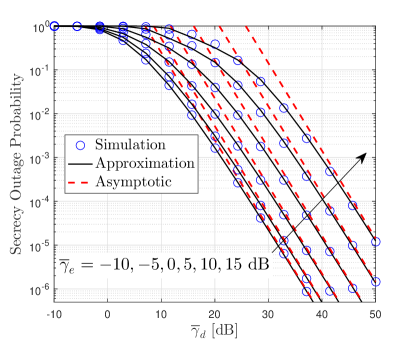
Figure 1: $P_{\rm sop}$ versus $\overline{\gamma}_{d}$ for $m_{d}=m_{e}=2.5$, $k_{d}=k_{e}=2$, and $R_{s}=1$.

From Fig. 2, for $k_{d}=1.5$, the slope of ASOP changes for $m_{d}=0.5,1$, and becomes constant for $m_{d}=2,2.5$, which shows that the secrecy diversity order is $\min\{k_{d},m_{d}\}$. Fig. 3 plots the SOP versus $\overline{\gamma}_{d}$ for different $k_{d}=m_{d}$ values. The ASOP is not a linear function with respect to $\overline{\gamma}_{d}$ in dB, while the slope of ASOP changes very slowly in the high $\overline{\gamma}_{d}$ region.

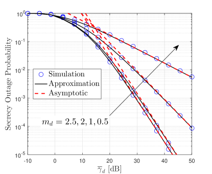
Figure 2: $P_{\rm sop}$ versus $\overline{\gamma}_{d}$ for $k_{d}=m_{e}=k_{e}=1.5$, $\overline{\gamma}_{e}=0$ dB, and $R_{s}=1$.

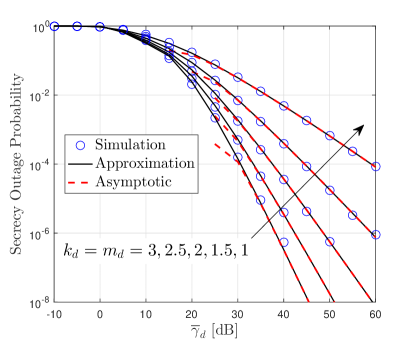
Figure 3: $P_{\rm sop}$ versus $\overline{\gamma}_{d}$ for $m_{e}=k_{e}=2$, $\overline{\gamma}_{e}=5$ dB, and $R_{s}=1$.

VI Conclusion

In this letter, a simple SOP expression was derived with a high accuracy for a small average SNR of the wiretap channel. Although the matching becomes worse for a large average SNR of the wiretap channel, the approximate SOP converges to the exact SOP with increasing the average SNR of the main channel. To obtain the secrecy diversity order, we also derived the asymptotic expression for the SOP valid in the high SNR region of the main channel. The ASOP expression also shows that the ASOP for $k_{d}=m_{d}$ is not a linear function with respect to $\overline{\gamma}_{d}$ in dB, despite the slowly changing slope in high SNRs.

References

[1]
P. S. Bithas, N. C. Sagias, P. T. Mathiopoulos, G. K. Karagiannidis, and A. A. Rontogiannis, “On the performance analysis
of digital communications over generalized- fading channels,” IEEE Commun. Lett., vol. 10, no. 5, pp. 353-355, May
2006.
[2]
A. Laourine, M.-S. Alouini, S. Affes, and A. Stephenne, “On the capacity of generalized- fading channels,” IEEE Trans. Wireless Commun., vol. 7, no. 7, pp. 2441-2445, Jul. 2008.
[3]
H. Y. Lateef, M. Ghogho, and D. McLernon, “On the performance analysis of multi-hop cooperative relay networks over
generalized- fading channels,” IEEE Commun. Lett., vol. 15, no. 9, pp. 968-970, Sep. 2011.
[4]
S. Atapattu, C. Tellambura, and H. Jiang, “A mixture Gamma distribution to model the SNR of wireless channels,” IEEE
Trans. Wireless Commun., vol. 10, no. 12, pp. 4193-4203, Dec. 2011.
[5]
M. Bloch, J. Barros, M. R. D. Rodrigues, and S. W. McLaughlin, “Wireless information-theoretic security,” IEEE Trans. Inf. Theory, vol. 54, no. 6, pp. 2515-2534, Jun. 2008.
[6]
H. Zhao, Y. Tan, G. Pan, Y. Chen, and N. Yang, “Secrecy outage on transmit antenna selection/maximal ratio combining in MIMO cognitive radio networks,” IEEE Trans. Veh. Technol., vol. 65, no. 12, pp. 10236-10242, Dec. 2016.
[7]
Y. Liu, Z. Qin, M. Elkashlan, Y. Gao, and L. Hanzo, “Enhancing the physical layer security of non-orthogonal multiple access in large-scale networks,” IEEE Trans. Wireless Commun., vol. 16, no. 3, pp. 1656-1672, Mar. 2017.
[8]
W. Zeng, J. Zhang, S. Chen, K. P. Peppas, and B. Ai, “Physical layer security over fluctuating two-ray fading channels,” IEEE Trans. Veh. Technol., vol. 67, no. 9, pp. 8949-8953, Sep. 2018.
[9]
J. P. Pena-Martin, J. M. Romero-Jerez, and F. J. Lopez-Martinez, “Generalized MGF of Beckmann fading with applications to wireless communications performance analysis,” IEEE Trans. Commun., vol. 65, no. 9, pp. 3933-3943, Sep. 2017.
[10]
X. Liu, “Outage probability of secrecy capacity over correlated lognormal fading channels,” IEEE. Commun. Lett., vol. vol. 17, no. 2, pp. 289-292, Feb. 2013.
[11]
G. C. Alexandropoulos, and K. P. Peppas, “Secrecy outage analysis over correlated composite Nakagami-/Gamma fading channels,” IEEE. Commun. Lett., vol. 22. no. 1, pp. 77-80, Jan. 2018.
[12]
H. Lei, H. Zhang, I. S. Ansari, C. Gao, Y. Guo, G. Pan, and K. A. Qaraqe, “Performance analysis of physical layer security over generalized- fading channels using a mixture Gamma distribution,” IEEE. Commun. Lett., vol. 20, no. 2, pp. 408-411, Feb. 2016.
[13]
H. Lei, I. S. Ansari, C. Gao, Y. Guo, G. Pan, and K. A. Qaraqe, “Secrecy performance analysis of single-input multiple-output
generalized- fading channels,” Front. Inform. Technol. Electron. Eng., vol. 17, no. 10, pp. 1074-1084, Oct. 2016.
[14]
L. Wu, L. Yang, J. Chen, and M.-S. Alouini, “Physical layer security for cooperative relaying over generalized- fading
channels,” IEEE Wireless Commun. Lett., vol. 7, no. 4, pp. 606-609, Aug. 2018.
[15]
Z. Wang, H. Zhao, S. Wang, J. Zhang, and M.-S. Alouini, “Secrecy analysis in SWIPT systems over generalized- fading channels,” IEEE Commun. Lett., vol. 23, no. 5, pp. 834-837, May 2019.
[16]
L. Kong, and G. Kaddoum, “Secrecy characteristics with assistance of mixture Gamma distribution,” IEEE Wireless Commun. Lett., accepted for publication. DOI: 10.1109/LWC.2019.2907083.
[17]
H. Lei, I. S. Ansari, C. Gao, Y. Guo, G. Pan, and K. A. Qaraqe, “Physical-layer security over generalised- fading channels,” IET Commun., vol. 10, no. 16, pp. 2233-2237, Nov. 2016.
[18]
H. Lei C. Gao, I. S. Ansari, Y. Guo, G. Pan, and K. A. Qaraqe, “On physical-layer security over SIMO generalized-
fading channels,” IEEE Trans. Veh. Technol., vol. 65, no. 9, pp. 7780-7785, Sep. 2016.
[19]
G. Pan, C. Tang, X. Zhang, T. Li, Y. Weng, and Y. Chen, “Physical-layer security over non-small-scale fading channels,” IEEE Trans. Veh. Technol., vol. 65, no. 3, pp. 1326-1339, Mar. 2016.
[20]
J. M. Holtzman, “A simple, accurate method to calculate spread multiple access error probabilities,” IEEE Trans. Commun., vol. 40, no. 3, pp. 461-464, Mar. 1992.
[21]
I. S. Gradshteyn, I. M. Ryzhik, Table of Integrals, Series, and Products, 7th edition. Academic Press, 2007.
[23]
H. Zhao, L. Yang, A. S. Salem, and M.-S. Alouini, “Ergodic capacity under power adaption over Fisher-Snedecor fading channels,” IEEE Commun. Lett., vol. 23, no. 3, pp. 546-549, Mar. 2019.