Repeated interactions and quantum stochastic thermodynamics at strong coupling

Abstract

The thermodynamic framework of repeated interactions is generalized to an arbitrary open quantum system in contact with a heat bath. Based on these findings the theory is then extended to arbitrary measurements performed on the system. This constitutes a direct experimentally testable framework in strong coupling quantum thermodynamics. By construction, it provides many quantum stochastic processes and quantum causal models with a consistent thermodynamic interpretation. The setting can be further used, for instance, to rigorously investigate the interplay between non-Markovianity and nonequilibrium thermodynamics.

Introduction.— Formulating the laws of quantum thermodynamics forces us to rethink many assumptions, which are traditionally taken for granted. In particular, small systems are dominated by fluctuations and in general they do not interact weakly with a Markovian heat bath. Also the desire to monitor and manipulate quantum systems adds another layer of complexity due to the non-trivial effect of quantum measurements.

In this Letter we present a unified thermodynamic framework, which overcomes the assumption of a weakly coupled, Markovian heat bath and which allows to include nonequilibrium resources and quantum measurements. These nonequilibrium resources are a set of small, externally prepared systems – called ‘units’ in the following – which are sequentially put into contact with the system under study. This setup is known as the ‘repeated interaction framework’ or ‘collisional model’ and it has recently attracted much attention in quantum thermodynamics Bruneau et al. (2010); Horowitz (2012); Horowitz and Parrondo (2013); Barra (2015); Uzdin et al. (2016); Pezzutto et al. (2016); Strasberg et al. (2017); Benoist et al. (2018); Manzano et al. (2018); Chiara et al. (2018); Cresser (2019); Seah et al. (2019); Bäumer et al. (2019). However, the coupling to an additional external heat bath (typically present in an experiment) was mostly ignored, a weakly coupled Markovian one was only treated in Refs. Bruneau et al. (2010); Strasberg et al. (2017); Cresser (2019). Based on recent progress in strong coupling thermodynamics Seifert (2016); Strasberg and Esposito (2019), we will show that even the assumption of a weakly coupled macroscopic heat bath can be completely overcome.

Afterwards, following the operational approach to quantum stochastic thermodynamics Strasberg (2019); Strasberg and Winter (2019), we will show how to explicitly take into account measurements into the thermodynamic description. This constitutes a crucial step in strong coupling quantum thermodynamics where different strategies were used to arrive at many interesting conclusions Campisi et al. (2009); Esposito et al. (2010); Takara et al. (2010); Schaller et al. (2013); Gallego et al. (2014); Esposito et al. (2015a, b); Gelbwaser-Klimovsky and Aspuru-Guzik (2015); Strasberg et al. (2016); Bruch et al. (2016); Katz and Kosloff (2016); Ludovico et al. (2016); Newman et al. (2017); Mu et al. (2017); Ludovico et al. (2018); Schaller et al. (2018); Strasberg et al. (2018); Perarnau-Llobet et al. (2018); Bruch et al. (2018); Whitney (2018); Restrepo et al. (2018); Dou et al. (2018); Schaller and A (2018); Guarnieri et al. (2019). However, all strategies rely on a formalism without any explicit measurements, thus making them hard to test and compare . In contrast, our theory is in principle immediately testable in a lab as it only requires to measure the system. Finally, we rigorously connect our thermodynamic framework to the field of quantum non-Markovianity.

Setting.— We start by considering a system $S$ coupled to a bath $B$ described by the Hamiltonian $H_{SB}(\lambda_{t})=H_{S}(\lambda_{t})+V_{SB}+H_{B}$, where $\lambda_{t}$ denotes an externally specified driving protocol (e.g., a laser field) and $V_{SB}$ denotes the system-bath interaction Hamiltonian. To this setup we add the framework of repeated interactions specified by the following global Hamiltonian:

$$H_{\text{tot}}(\lambda_{t})=H_{SB}(\lambda_{t})+\sum_{k=0}^{n}V_{SU(k)}(\lambda_{t}).$$ (1)

Here, $V_{SU(k)}(\lambda_{t})$ describes the time-dependent coupling between the system and unit $U(k)$, $k\in\{0,\dots,n\}$, which is designed in such a way that at most one unit interacts with the system at a given time. Specifically, if we denote the interaction interval between the system and the $k$’th unit by $I_{k}\equiv[t_{k},t_{k+1})$, then $V_{SU(k)}(\lambda_{t})=0$ for all $t\notin I_{k}$. Within $I_{k}$ the time-dependence as specified by $\lambda_{t}$ is arbitrary. Furthermore, we temporarily assume the bare unit Hamiltonian to be degenerate, i.e., $H_{U(k)}\sim 1_{U(k)}$. The problem is completely specified by fixing the global initial state, which is assumed to be of the form

$$\rho_{\text{tot}}(t_{0}^{-})=\pi_{SB}(\lambda_{0})\otimes\rho_{U(0)}\otimes\dots\otimes\rho_{U(n)}.$$ (2)

Here and in general we use the notation $t^{\pm}$ to denote the time $t\pm\epsilon$ in the limit where $\epsilon>0$ becomes immeasurably small. Furthermore, $\pi_{X}=e^{-\beta H_{X}}/{\cal{Z}}_{X}$ denotes the equilibrium Gibbs state of some system $X$ at inverse temperature $\beta$ (perhaps depending on the value of some driving protocol). Finally, the initial state of the units is arbitrary but uncorrelated. A sketch of the present setup is shown in Fig. 1. We remark that various extensions are possible as discussed at the end of this Letter.

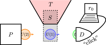
Figure 1: A system $S$ is in contact with a bath initialized at temperature $T$ (we do not imply that the bath must be kept at a well-defined temperature at later times). In a preparation apparatus $P$ units $U(k)$ are sequentially produced, which interact with the system when they enter the shaded grey area, and which are afterwards detected in $D$ giving rise to the measurement outcome $r_{k}$ (properly introduced later on in the text). Note that each unit can be different in principle. We also remark that the description of the units does not need to be taken literally in the sense that they are merely ‘ancillas’ required for a consistent thermodynamic description of a non-Markovian quantum stochastic process as introduced later on.

Below we will need the notion of the ‘Hamiltonian of mean force’, an old concept Kirkwood (1935) (see also Refs. Seifert (2016); Strasberg and Esposito (2019); Campisi et al. (2009)), which is defined via the reduced equilibrium state of a bipartite system $XB$. Specifically,

$$\pi_{X}^{*}\equiv\mbox{tr}_{B}\{\pi_{XB}\}\equiv\frac{e^{-\beta H_{X}^{*}}}{{\cal{Z}}_{X}^{*}},~{}~{}~{}{\cal{Z}}_{X}^{*}\equiv\frac{{\cal{Z}}_{XB}}{{\cal{Z}}_{B}}.$$ (3)

Note that $\pi_{X}^{*}\neq\pi_{X}$ in general. In addition, $H_{X}^{*}$ depends on the inverse temperature $\beta$ and (possibly) a control parameter. Notice that the Hamiltonian of mean force for the system and all units simplifies as at any given time at most one unit is physically coupled to the system, e.g., for $t\in I_{k}$, $H_{SU(\textbf{n})}^{*}(\lambda_{t})=H_{SU(k)}^{*}(\lambda_{t})$. Here and in general we use $U(\textbf{n})$ to denote the entire sequence of units from $U(0)$ to $U(n)$.

The average rate of injected work (the power) has two contributions. For $t\in I_{k}$ we define

$$\dot{W}_{S}(t) ={\left\langle{\frac{\partial H_{S}(\lambda_{t})}{\partial t}}\right\rangle}(t),$$ (4)

$$\dot{W}_{SU(k)}(t) ={\left\langle{\frac{\partial V_{SU(k)}(\lambda_{t})}{\partial t}}\right\rangle}(t),$$ (5)

where ${\left\langle{\dots}\right\rangle}(t)$ denotes a quantum statistical average at time $t$. It follows that the total mechanical work performed on the system up to time $t$ is

$$W(t) =\int_{t_{0}^{-}}^{t}ds[\dot{W}_{S}(s)+\sum_{k}\dot{W}_{SU(k)}(s)]$$ (6)

$$={\left\langle{H_{\text{tot}}(\lambda_{t})}\right\rangle}(t)-{\left\langle{H_{\text{tot}}(\lambda_{0}^{-})}\right\rangle}(t_{0}^{-}).$$

Note that this definition of average mechanical work is widely accepted even in the strong coupling regime Strasberg and Esposito (2019); Esposito et al. (2010); Takara et al. (2010); Esposito et al. (2015a, b); Strasberg et al. (2016); Ludovico et al. (2016); Strasberg et al. (2018); Perarnau-Llobet et al. (2018); Whitney (2018); Dou et al. (2018) as it is directly related to the change in internal energy of the universe (i.e., the system, the bath and all units all together).

Strong coupling repeated interactions framework.— We start by introducing the basic concept of a nonequilibrium free energy adapted to the strong coupling regime Seifert (2016); Strasberg and Esposito (2019),

$$F_{X}(t)\equiv\mbox{tr}_{X}\{\rho_{X}(t)[H_{X}^{*}(\lambda_{t})+\beta^{-1}\ln\rho_{X}(t)]\}.$$ (7)

In the weak coupling limit, where $H_{X}^{*}(\lambda_{t})\approx H_{X}(\lambda_{t})$, this definition reduces to the conventional one. The slight modification allows us to express the second law even at strong coupling and even in presence of the system-unit interactions in the conventional way ($k_{B}\equiv 1$):

$$\Sigma(t)\equiv\beta[W(t)-\Delta F_{SU(\textbf{n})}(t)]\geq 0.$$ (8)

Here, $\Sigma(t)$ denotes the entropy production and $\Delta F_{SU(\textbf{n})}(t)\equiv F_{SU(\textbf{n})}(t)-F_{SU(\textbf{n})}(t_{0}^{-})$. Positivity of the second law follows by confirming that

$$\Sigma(t)=D[\rho_{\text{tot}}(t)\|\pi_{\text{tot}}(\lambda_{t})]-D[\rho_{SU(\textbf{n})}(t)\|\pi_{SU(\textbf{n})}^{*}(\lambda_{t})],$$ (9)

where $D[\rho\|\sigma]=\mbox{tr}\{\rho(\ln\rho-\ln\sigma)\}\geq 0$ is the quantum relative entropy. Hence, $\Sigma(t)$ is positive by monotonicity of relative entropy Uhlmann (1977); Ohya and Petz (1993). The derivation uses only Eq. (2) and the unitary dynamics, which implies for the von Neumann entropy $S[\rho_{\text{tot}}(0)]\equiv-\mbox{tr}\{\rho_{\text{tot}}(0)\ln\rho_{\text{tot}}(0)\}=S[\rho_{\text{tot}}(t)]$. It is lengthy but straightforward and hence not displayed here.

Equation (8) corresponds to the second law if we regard the system and all units as one big system and explicitly keep their correlations in the description. In practice it often turns out that keeping the information about all units and all their correlations is superfluous (compare also with the discussion in Ref. Strasberg et al. (2017)). Thus, at time $t_{n+1}^{-}$ after the $n$’th interaction but before the $(n+1)$’th interaction, where the system is decoupled from all units, the following second law is practically more meaningful,

$$\Sigma_{S}(t_{n+1}^{-}) =\beta[W(t_{n+1}^{-})-\Delta F_{S}(t_{n+1}^{-})]+\sum_{k=0}^{n}\Delta S[\rho_{U(k)}]$$

$$\geq\Sigma(t_{n+1}^{-})\geq 0.$$ (10)

Here, we added a subscript $S$ to indicate that this is the entropy production from the system point of view ignoring superfluous information about the units. To arrive at Eq. (10), we used subadditivity of entropy and $H_{U(k)}\sim 1_{U(k)}$. In contrast to Eq. (8) it contains only the change in the marginal von Neumann entropy of the units. The entropy production per interaction interval $I_{n}$ is then given by

$$\begin{split}\Sigma_{S}&(t_{n+1}^{-})-\Sigma_{S}(t_{n}^{-})=\\ &\beta[W(t_{n+1}^{-})-W(t_{n}^{-})-F_{S}(t_{n+1}^{-})+F_{S}(t_{n}^{-})]\\ &+S[\rho_{U(n)}(t_{n+1}^{-})]-S[\rho_{U(n)}(t_{n}^{-})].\end{split}$$ (11)

It is the strong coupling generalization of the second law in the repeated interaction framework, see Eq. (49) in Ref. Strasberg et al. (2017). Interestingly, in contrast to the Markovian weak coupling situation, we cannot ensure the positivity of this expression. This is similar to the classical case Strasberg and Esposito (2019) and we will connect it to the notion of non-Markovianity later on. But first we will advance conceptually by introducing explicit measurements in the description.

Quantum stochastic thermodynamics at strong coupling.— We consider the case where the experimenter measures the state of the unit after the interaction with the system as indicated in Fig. 1 (i.e., $V_{SU(n)}(\lambda_{t})=0$ at the time $t$ of the measurement). By doing so, she can gather valuable information about the state of the system. In a moment we will also show that this allows her to implement arbitrary generalized measurements on the system and that the resulting theory can be fruitfully linked to the study of quantum stochastic processes and quantum causal models.

Mathematically, we denote the measurement result of the $k$’th unit by $r_{k}$ and associate a positive operator $P_{r_{k}}$ to it, which fulfills the normalization condition $\sum_{r_{k}}P_{r_{k}}^{2}=1_{U(k)}$. The state of the unit then changes according to the map ${\cal{P}}_{r_{k}}\rho_{U(k)}\equiv P_{r_{k}}\rho_{U(k)}P_{r_{k}}\equiv\tilde{\rho}_{U(k)}(r_{k})$. Notice that $\tilde{\rho}_{U(k)}(r_{k})$ is a subnormalized state with the probability $p(r_{k})=\mbox{tr}_{U(k)}\{\tilde{\rho}_{U(k)}(r_{k})\}$ as its norm. After multiple units were subjected to their respective measurements giving results $\textbf{r}_{n}\equiv(r_{n},\dots,r_{1},r_{0})$, the global subnormalized state reads

$$\tilde{\rho}_{\text{tot}}(\textbf{r}_{n},t_{n+1}^{-})=\left(\prod_{k=0}^{n}{\cal{P}}_{r_{k}}{\cal{U}}_{k+1,k}\right)\rho_{\text{tot}}(t_{0}^{-}).$$ (12)

Here, ${\cal{U}}_{k+1,k}$ describes the global unitary evolution from $t_{k}^{-}$ (shortly before the $k$’th unit starts interacting with the system) to $t_{k+1}^{-}$. Due to the fact that the measurement always acts after the interaction we can also write

$$\tilde{\rho}_{\text{tot}}(\textbf{r}_{n},t_{n+1}^{-})=\left(\prod_{k=0}^{n}{\cal{P}}_{r_{k}}\right)\rho_{\text{tot}}(t_{n+1}^{-}),$$ (13)

where $\rho_{\text{tot}}(t_{n+1}^{-})={\cal{U}}_{n+1,0}\rho_{\text{tot}}(t_{0}^{-})$ is the global time-evolved state without any measurements. This allows us to confirm the useful relation

$$\sum_{\textbf{r}_{n}}\tilde{\rho}_{SB}(\textbf{r}_{n},t_{n+1}^{-})=\rho_{SB}(t_{n+1}^{-}),$$ (14)

i.e., the average system-bath state does not change due to the measurements. This is not true for the units.

Inspired by Ref. Strasberg (2019), we now introduce the following thermodynamic definitions along a single trajectory characterized by the measurement results $\textbf{r}_{n}$. First, for $t\in I_{n}$ the stochastic power $\dot{w}_{S}(\textbf{r}_{n},t)$ and $\dot{w}_{SU(n)}(\textbf{r}_{n-1},t)$ are simply obtained from Eqs. (4) and (5) by replacing the average over the unconditional state $\rho_{SU(\textbf{n})}(t)$ with an average over the conditional state $\rho_{SU(\textbf{n})}(\textbf{r}_{n},t)$. Notice that $\dot{w}_{SU(n)}(\textbf{r}_{n-1},t)$ does not depend on the last measurement outcome $r_{n}$ because by construction the measurement ${\cal{P}}_{r_{n}}$ acts after the $n$th unit has interacted with the system. Therefore, together with Eq. (14) we immediately obtain the relations $\sum_{\textbf{r}_{n}}p(\textbf{r}_{n})\dot{w}_{S}(\textbf{r}_{n},t)=\dot{W}_{S}(t)$ and $\sum_{\textbf{r}_{n}}p(\textbf{r}_{n})\dot{w}_{SU(n)}(\textbf{r}_{n-1},t)=\dot{W}_{SU(n)}(t)$. Second, we have to generalize the nonequilibrium free energy to the stochastic case, which becomes

$$\begin{split}f_{SU(\textbf{n})}(\textbf{r}_{n},t)\equiv&~{}{\left\langle{H_{SU(\textbf{n})}^{*}(\lambda_{t})}\right\rangle}(\textbf{r}_{n},t)\\ &+T\left\{\ln p(\textbf{r}_{n})-S[\rho_{SU(\textbf{n})}(\textbf{r}_{n},t)]\right\},\end{split}$$ (15)

where ${\left\langle{\dots}\right\rangle}(\textbf{r}_{n},t)$ denotes an average with respect to the conditional state. An essential difference compared to definition (7) is the appearence of the stochastic entropy $-\ln p(\textbf{r}_{n})$ associated to the measurement results obtained with probability $p(\textbf{r}_{n})=\mbox{tr}\{\tilde{\rho}_{\text{tot}}(\textbf{r}_{n},t)\}$. A similar but not identical construction is used in classical stochastic thermodynamics Seifert (2005), compare with the discussion in Refs. Strasberg (2019); Strasberg and Winter (2019). In contrast to the stochastic work, we have in general $\sum_{\textbf{r}_{n}}p(\textbf{r}_{n})f_{SU(\textbf{n})}(\textbf{r}_{n},t)\neq F_{SU(\textbf{n})}(t)$. Finally, we introduce the stochastic entropy production

$$\sigma(\textbf{r}_{n},t)\equiv\beta[w(\textbf{r}_{n},t)-\Delta f_{SU(\textbf{n})}(\textbf{r}_{n},t)].$$ (16)

As in classical stochastic thermodynamics, it can be negative along a single trajectory Seifert (2012); Van den Broeck and Esposito (2015). However, we will now prove that on average $\sum_{\textbf{r}_{n}}p(\textbf{r}_{n})\sigma(\textbf{r}_{n},t)\geq 0$, which demonstrates the thermodynamic consistency of our strong coupling quantum stochastic framework.

As a consequence of Eq. (14) and our previously derived second law (8), we confirm that

$$\sum_{\textbf{r}_{n}}p(\textbf{r}_{n})\sigma(\textbf{r}_{n},t)-\Sigma(t)=$$ (17)

$$\sum_{\textbf{r}_{n}}p(\textbf{r}_{n})\left\{S[\rho_{SU(\textbf{n})}(\textbf{r}_{n},t)]-\ln p(\textbf{r}_{n})\right\}-S[\rho_{SU(\textbf{n})}(t)].$$

This quantifies the change in informational entropy of all constituents (system, units and the classical memory) due to the big joint measurement (13). Its positivity follows from the Lemma in Ref. Strasberg (2019), which simply combines Theorem 11 of Ref. Jacobs (2014) and Theorem 11.10 of Ref. Nielsen and Chuang (2000) and which can be interpreted as the second law for a quantum measurement. Hence, we conclude

$$\sum_{\textbf{r}_{n}}p(\textbf{r}_{n})\sigma(\textbf{r}_{n},t)\geq\Sigma(t)\geq 0.$$ (18)

As before, the (averaged) stochastic entropy production $\sigma(\textbf{r}_{n},t)$ contains the information about all the correlations in the units, which is typically not needed. Using subadditivity of entropy, it is again possible to arrive at expressions similar to Eq. (10). Note that, depending on the experimental situation, one could decide to not only discard information about the unit correlations, but also about the measurement results $\textbf{r}_{n}$.

This concludes the formal part of the Letter, where we have introduced a consistent notion of work, nonequilibrium free energy and entropy production along a single run of an experiment regardless of any details of the system-bath coupling. It is instructive to connect the present picture to the theory of quantum causal models and quantum stochastic processes. If we consider the limit of an instantaneous system-unit interaction, ideally described by a coupling of the form $V_{SU(k)}(\lambda_{t})=v_{k}\delta(t-t_{k})$, we can write the system-bath dynamics as

$$\tilde{\rho}_{SB}(\textbf{r}_{n},t_{n+1}^{-})=\left(\prod_{k=0}^{n}{\cal{U}}^{SB}_{k+1,k}{\cal{A}}_{r_{k}}\right)\rho_{SB}(t_{0}^{-}).$$ (19)

Here, ${\cal{U}}^{SB}_{k+1,k}$ is the unitary time evolution generated by $H_{SB}(\lambda_{t})$ and the completely positive map ${\cal{A}}_{r_{k}}$ is defined via its action ${\cal{A}}_{r_{k}}\rho_{S}=\mbox{tr}_{U}\{{\cal{P}}_{r_{k}}[e^{-iv_{k}\hbar}\rho_{S}\rho_{U(k)}e^{iv_{k}/\hbar}]\}$ on an arbitrary system state $\rho_{S}$. In this context ${\cal{A}}_{r_{k}}$ is also known as an ‘instrument’ describing the most general state transformation possible in quantum mechanics Holevo (2001); Wiseman and Milburn (2010). The application of a set of instruments ${\cal{A}}_{r_{0}},\dots,{\cal{A}}_{r_{n}}$ to an open quantum system defines a general quantum stochastic process (or quantum causal model), which can be formally represented by a ‘quantum comb’ or ‘process tensor’ Chiribella et al. (2008, 2009); Costa and Shrapnel (2016); Oreshkov and Giarmatzi (2016); Pollock et al. (2018a); Milz et al. (2017). The sole difference compared to the most general case is that we do not allow for real-time feedback control, i.e., the instruments ${\cal{A}}_{r_{k}}$ are not allowed to depend on the previous results $\textbf{r}_{k-1}$, otherwise Eq. (14) would no longer be true. Whether the present framework can be extended to arbitrary real-time feedback control as in the Markovian case Strasberg (2019); Strasberg and Winter (2019) remains an open question.

Thermodynamic signatures of non-Markovianity.— We now turn towards an important application linking the field of quantum thermodynamics and quantum non-Markovianity Rivas et al. (2014); Breuer et al. (2016) in a rigorous way. As recognized below Eq. (11), at strong coupling we cannot ensure that the entropy production is positive in every time-interval $[t_{\ell},t_{k})$ for $t_{\ell}>t_{k}>t_{0}$. There have been repeated claims in the literature that negative entropy production rates indicate non-Markovianity Argentieri et al. (2014); Bhattacharya et al. (2017); Marcantoni et al. (2017); Popovic et al. (2018); Thomas et al. (2018); Bhattacharya et al. (2019). Doubts were raised in Refs. Strasberg and Esposito (2019) since the definitions for entropy production rates used in Refs. Argentieri et al. (2014); Bhattacharya et al. (2017); Marcantoni et al. (2017); Popovic et al. (2018); Thomas et al. (2018); Bhattacharya et al. (2019) do not yield an overall positive entropy production when integrated from the initial time $t_{0}$ to any final time $t>t_{0}$. Moreover, they can be even negative for Markovian dynamics Strasberg and Esposito (2019).

On the other hand, for a suitable notion of entropy production based on the Hamiltonian of mean force progress was achieved for classical dynamics Strasberg and Esposito (2019). In there, the situation of a strongly coupled system prepared in an arbitrary nonequilibrium state was considered (no repeated interactions were present). Then, it was shown that Markovian dynamics necessarily imply a positive entropy production rate if the system is undriven (i.e., $\lambda_{t}=$ constant). In our quantum formalism the system is initially in equilibrium such that its state does not change when undriven and left on its own. However, we can link the present picture to the classical case by realizing that we can use the very first unit $U(0)$ to prepare the system in an arbitrary nonequilibrium state via a short control operation. This preparation procedure has a thermodynamic cost captured by the always positive entropy production $\Sigma_{S}(t)=\beta W_{SU}(t)-\beta\Delta F_{S}(t)-\beta\Delta S[\rho_{U(0)}]\geq 0$, compare with Eq. (10). After the system-unit interaction, the system is left on its own and the entropy production in between any two times $t_{2}>t_{1}>t_{0}$ reads

$$\begin{split}\Sigma_{S}(t_{2})-\Sigma_{S}(t_{1})&=-\beta[F_{S}(t_{2})-F_{S}(t_{1})]\\ &=D[\rho_{S}(t_{1})\|\pi_{S}^{*}]-D[\rho_{S}(t_{2})\|\pi_{S}^{*}].\end{split}$$ (20)

This quantifies the dissipation associated with the relaxation dynamics of the system. Equation (20) is positive if the dynamics are Markovian and if $\pi_{S}^{*}$ is a steady state of the dynamics at any time $t$. Interestingly, the latter point can be shown rigorously based on the definition of Markovianity from Ref. Pollock et al. (2018b), which is adapted to the situation of a general quantum stochastic process as used here. This is proven in the Appendix A. Thus, $\Sigma_{S}(t_{2})-\Sigma_{S}(t_{1})\geq 0$ for a Markov process in complete analogy to the classical result Strasberg and Esposito (2019). This opens up the door to investigate the interplay between entropy production and non-Markovianity in a mathematically and thermodynamically rigorous sense for quantum systems.

Further applications.— The ability to analyse general non-Markovian quantum processes from a thermodynamic perspective will find applications in various areas. One example is sequential quantum metrology Giovanneti et al. (2011). Specifically, a particular intriguing parameter to estimate is the temperature of a system. Much progress has been achieved to understand it from the perspective of metrology Mehboudi et al. (2019), but the thermodynamic costs of thermometry were not yet explored. With the recent progress in the design of optimal quantum probes Correa et al. (2015) and strong-coupling thermometry Correa et al. (2017), the present Letter opens up the possibility to thermodynamically analyse many scenarios in metrology and thermometry. Furthermore, recent progress shows how to unambigously detect quantum features in quantum stochastic processes Smirne et al. (2018); Strasberg and Díaz (2019); Milz et al. (2019). Since quantum thermodynamics is still in the search for clear observable quantum effects induced by coherence González et al. (2019), the present letter will allow to rigorously address such questions. Furthermore, originally used to understand Nobelprize-winning experiments Sayrin et al. (2011); Zhou et al. (2012) in quantum optics from a thermodynamic perspective Strasberg (2019), the present framework can be used to explore more general cases where the system is not a high-quality cavity and has substantial losses or is coupled to other cavities. Also the units do not have to be identical, which opens up the possibility to, e.g., thermodynamically analyse single-photon distillation experiments Daiss et al. (2019) where an atom in a cavity is first probed by a weak coherent pulse (unit 1) followed by a measurement (modeled by unit 2) to herald the photon distillation. Quite generally, the present setup is even relevant for experiments in the Markovian regime, if detailed control about all system parts is not possible. Finally, the present framework can be combined with the traditional picture of scattering theory and, following Ref. Strasberg et al. (2017), it allows to investigate Maxwell’s demon and Landauer’s principle at strong coupling.

Extensions.— As detailed in Appendix B, the present framework can be extended into various directions: the Hamiltonian of the units does not need to be degenerate, the initial state of the units can be correlated, and the general identities (8), (10) and (18) still hold in the case where the system-bath coupling is time-dependent. In the last case, however, the theory is no longer ‘operational’ in the sense that explicit knowledge about the state of the bath is necessary, which is hardly accessible. Similarly, we show in Appendix B how to treat multiple heat baths. Unfortunately, also in that case the state of the system and units does not suffice to have access to all thermodynamic quantities .

Concluding remarks.— The present contribution establishes a consistent thermodynamic framework – even along a single trajectory recorded in an experiment – for a system in contact with an arbitrary bath and additionally subjected to arbitrary nonequilibrium resources interacting one by one with the system. This pushes the applicability of nonequilibrium thermodynamics far beyond its traditional scope. Furthermore, the present work also demonstrates how quantum stochastic thermodynamics departs from its classical version in the strong coupling regime Seifert (2016); Jarzynski (2017); Miller and Anders (2017); Strasberg and Esposito (2017, 2019). While the basic concepts at the unmeasured level are similar, any possible measurement strategy has a non-trivial influence on the description in the quantum regime, even on average. For instance, in general there is a strict inequality on the left hand side of Eq. (18). This is not a deficiency of our theory, but a necessary ingredient, which can be already recognized at the level of the work statistics Perarnau-Llobet et al. (2017). Quantum stochastic thermodynamics is more than a mere extension of its classical counterpart. The present operational approach is, however, flexible enough to reproduce the unmeasured picture: it is recovered by choosing the trivial but legitimiate measurement operator $P_{r_{k}}=1_{U(k)}$, i.e., the identity. Then, the stochastic entropy production $\sigma(\textbf{r}_{n})$ reduces to $\Sigma$.

Acknowledgments.— I thank Kavan Modi for illuminating initial discussions. This research was financially supported by the DFG (project STR 1505/2-1) and also the Spanish MINECO FIS2016-80681-P (AEI-FEDER, UE).

Appendix A Steady state of an undriven quantum Markov process

According to Ref. Pollock et al. (2018b), a Markov process is characterized by a set of completely positive and trace-preserving maps $\{\Lambda(t_{\ell},t_{k})|t_{\ell}>t_{k}\}$ such that the normalized state conditioned on an arbitrary sequence of control operations ${\cal{A}}_{0},{\cal{A}}_{1},\dots,{\cal{A}}_{n}$ can be written as

$$\rho(t_{n}^{+}|{\cal{A}}_{n},\dots,{\cal{A}}_{1},{\cal{A}}_{0})={\cal{A}}_{n}\Lambda(t_{n},t_{n-1})\dots\cal{A}_{1}\Lambda(t_{1},t_{0}){\cal{A}}_{0}\rho_{S}(t_{0}^{-}).$$ (21)

Notice that the composition law $\Lambda(t_{3},t_{1})=\Lambda(t_{3},t_{2})\Lambda(t_{2},t_{1})$ for $t_{3}>t_{2}>t_{1}$ (the ‘quantum Chapman-Kolmogorov equation’) automatically follows from that by realizing that the identity operation ${\cal{I}}$ is a legitimate control operation too.

By applying this to our problem, we immediately realize that we obtain the relation

$$\Lambda(t_{k},t_{0})\pi_{S}^{*}=\pi_{S}^{*}$$ (22)

for any $t_{k}>t_{0}$ and hence, the same holds for any intermediate map $\Lambda(t_{\ell},t_{k})$ ($t_{\ell}>t_{k}$). Note that the assumption of no driving as well as the particular form of the initial system-bath state [$\rho_{SB}(t_{0}^{-})=\pi_{SB}$] is crucial to arrive at this conclusion. Equation (20) of the main text can therefore be written as

$$D[\rho_{S}(t_{1})\|\pi_{S}^{*}]-D[\rho_{S}(t_{2})\|\pi_{S}^{*}]=D[\rho_{S}(t_{1})\|\pi_{S}^{*}]-D[\Lambda(t_{2},t_{1})\rho_{S}(t_{1})\|\Lambda(t_{2},t_{1})\pi_{S}^{*}].$$ (23)

Now, we can use that for a Markov process relative entropy is contractive Rivas et al. (2014); Breuer et al. (2016) to conclude that Eq. (20) of the main text is positive.

It is, of course, worth to point out that in general, for an initially correlated state of the form $\pi_{SB}$, there exists no such set of completely positive and trace-preserving maps $\{\Lambda(t_{\ell},t_{k})|t_{\ell}>t_{k}\}$. Obviously, this simply shows that one should not typically expect Markovian behaviour in strongly coupled systems. Nevertheless, in particular – and not necessarily uninteresting – limiting cases this can still be the case, e.g., in the limit of time-scale separation Strasberg and Esposito (2017), which allows in the quantum case to derive a Markovian master equation in a Polaron frame Schaller et al. (2013); Gelbwaser-Klimovsky and Aspuru-Guzik (2015); Strasberg et al. (2016).

Appendix B Extensions of strong coupling quantum stochastic thermodynamics

For later comparison, we start by listing the definitions of internal energy, heat flow and system entropy complementary to the definition of work and nonequilibrium free energy based on the assumptions of the main text (only one heat bath, energy degenerate units, no driving in the system-bath interaction). At the unmeasured level we have

$$E^{*}_{SU(\textbf{n})}(t) \equiv{\left\langle{H_{SU(\textbf{n})}^{*}(\lambda_{t})+\beta\partial_{\beta}H_{SU(\textbf{n})}^{*}(\lambda_{t})}\right\rangle}(t),$$ (24)

$$Q_{SU(\textbf{n})}(t) \equiv\Delta E^{*}_{SU(\textbf{n})}(t)-W(t),$$ (25)

$$S_{SU(\textbf{n})}(t) \equiv S[\rho_{SU(\textbf{n})}(t)]+\beta^{2}{\left\langle{\partial_{\beta}H_{SU(\textbf{n})}^{*}(\lambda_{t})}\right\rangle}(t).$$ (26)

Remember that $W(t)$ is the total work as defined in Eq. (6) of the main text and the letter $S$ without subscripts always denotes the von Neumann entropy $S(\rho)=-\mbox{tr}\{\rho\ln\rho\}$. Hence, we see that the thermodynamic entropy $S_{SU(\textbf{n})}(t)$ is not identical to the von-Neumann entropy in the strong coupling regime. Also note that $F_{SU(\textbf{n})}(t)=E^{*}_{SU(\textbf{n})}(t)-TS_{SU(\textbf{n})}(t)$ reproduces the definition of nonequilibrium free energy of the main text. The above definitions have been already discussed for a single system strongly coupled to a bath in the classical Seifert (2016); Jarzynski (2017); Miller and Anders (2017); Strasberg and Esposito (2017, 2019) and quantum Strasberg and Esposito (2019) case in the absence of any units. The second law of nonequilibrium thermodynamics can be expressed in the two alternative forms

$$\Sigma(t)=\beta[W(t)-\Delta F_{SU(\textbf{n})}(t)]=\Delta S_{SU(\textbf{n})}(t)-\beta Q_{SU(\textbf{n})}(t)\geq 0.$$ (27)

To extend the above definitions to the trajectory level, we have to replace the state $\rho_{SU(\textbf{n})}(t)$ by the conditional state $\rho_{SU(\textbf{n})}(\textbf{r}_{n},t)$ and we have to add the stochastic entropy of the detector $[-\ln p(\textbf{r}_{n})]$ to the definition of entropy. We denote this as

$$e^{*}_{SU(\textbf{n})}(\textbf{r}_{n},t) \equiv{\left\langle{H_{SU(\textbf{n})}^{*}(\lambda_{t})+\beta\partial_{\beta}H_{SU(\textbf{n})}^{*}(\lambda_{t})}\right\rangle}(\textbf{r}_{n},t),$$ (28)

$$q_{SU(\textbf{n})}(\textbf{r}_{n},t) \equiv\Delta e^{*}_{SU(\textbf{n})}(\textbf{r}_{n},t)-w(\textbf{r}_{n},t),$$ (29)

$$s_{SU(\textbf{n})}(\textbf{r}_{n},t) \equiv S[\rho_{SU(\textbf{n})}(\textbf{r}_{n},t)]+\beta^{2}{\left\langle{\partial_{\beta}H_{SU(\textbf{n})}^{*}(\lambda_{t})}\right\rangle}(\textbf{r}_{n},t)-\ln p(\textbf{r}_{n}).$$ (30)

Note that we naturally assume the notation $(\textbf{r}_{n},t)$ to imply a time $t$ where we have already measured the state of the $n$th unit (giving result $r_{n}$) but where the next $(n+1)$th unit was not yet measured. The stochastic entropy production can be again expressed in the two alternative forms

$$\sigma(\textbf{r}_{n},t)=\beta[w(\textbf{r}_{n},t)-\Delta f_{SU(\textbf{n})}(\textbf{r}_{n},t)]=\Delta s_{SU(\textbf{n})}(\textbf{r}_{n},t)-\beta q_{SU(\textbf{n})}(\textbf{r}_{n},t).$$ (31)

On average, $\sum_{\textbf{r}_{n}}p(\textbf{r}_{n})\sigma(\textbf{r}_{n},t)\geq 0$.

We will now investigate various extensions of the framework presented in the main text. We will be very explicit with the steps in Extension 4 (multiple heat baths) as it is the most general setting implying all the others (including the one of the main text). Therefore, for the Extensions 1 to 3 we limit ourselves to only pointing out some essential observations.

B.1 Extension 1: Driven system-bath interaction

In this case we allow that the system-bath interaction $V_{SB}=V_{SB}(\lambda_{t})$ depends on some externally prescribed time-dependent protocol $\lambda_{t}$. Such a setting is important, e.g., to model how a system is put into contact with a bath. Including this case only changes the definition of power [Eq. (4) in the main text] in an obvious way to

$$\dot{W}_{S}(t)=\mbox{tr}_{SB}\left\{\left[\frac{\partial H_{S}(\lambda_{t})}{\partial t}+\frac{\partial V_{SB}(\lambda_{t})}{\partial t}\right]\rho_{SB}(t)\right\}.$$ (32)

Despite being only a little formal change, this scenario implies that the power can no longer be computed based only on the knowledge of the system state $\rho_{S}(t)$, but in general requires to know the entire state $\rho_{SB}(t)$. This is problematic from an experimental point of view as the theory is no longer operational and also from a computational point of view it is very challenging. The stochastic generalization $\dot{w}_{S}(\textbf{r}_{n},t)$ of Eq. (32) simply uses the conditional state $\rho_{SB}(\textbf{r}_{n},t)$.

B.2 Extension 2: Correlated initial unit state

As will become clear in the detailed derivation below, the initial state of the units $\rho_{U(\textbf{n})}(t_{0}^{-})$ can indeed be arbitrary and does not need to be decorrelated. However, in practical applications this is often unnecessary and only complicates the theoretical treatment. Furthermore, deriving a simplified second law for the system alone [as in Eqs. (10) and (11) of the main text] becomes non-trivial then.

B.3 Extension 3: Energetic units

This generalization is slightly more subtle as the previous two when it comes to the trajectory level. The reason is that for energetically non-degenerate units the act of measurement, which requires to couple the microscopic unit to some macroscopic (not further specified) detection apparatus, can change the energy of the unit even on average unless the measurement operators $P_{r_{k}}$ commute with the unit Hamiltonian or the final unit state. While this is often the case in practice, see, e.g., Refs. Sayrin et al. (2011); Zhou et al. (2012), we are here interested in the most general scenario. Note that these subtleties were already discussed in greater detail in Ref. Strasberg (2019), compare also with the related (but not identical) concept of “quantum heat” introduced in Ref. Elouard et al. (2017).

To start with, nothing changes at the unmeasured level: Eqs. (24) to (27) remain true as usual. Now, to isolate the contribution steming solely from the energetic measurements of the unit due to the final measurement we define

$$q_{\text{meas}}(\textbf{r}_{n},t)\equiv e_{U(\textbf{n})}(\textbf{r}_{n},t)-E_{U(\textbf{n})}(t).$$ (33)

Here, $E_{U(\textbf{n})}(t)=\mbox{tr}_{U(\textbf{n})}\{H_{U(\textbf{n})}\rho_{U(\textbf{n})}(t)\}$ is the energy of all units evaluated with respect to the unmeasured state $\rho_{U(\textbf{n})}(t)=\mbox{tr}_{SB}\{{\cal{U}}_{t,t_{0}}\rho_{\text{tot}}(t_{0}^{-})\}$ of the units, whereas $e_{U(\textbf{n})}(t)=\mbox{tr}_{U(\textbf{n})}\{H_{U(\textbf{n})}\rho_{U(\textbf{n})}(\textbf{r}_{n},t)\}$ involves the measured state, compare also with Eq. (13) in the main text. Note that at the time of the measurement of the $n$th unit giving result $r_{n}$, the unit is physically decoupled from the system, i.e., we have $V_{SU(n)}(\lambda_{t})=0$ as indicated in Fig. 1 of the main text. We also remark that it is debated whether Eq. (33) should be counted as ‘heat’ or ‘work’. In fact, we will now split off this term from the total stochastic heat (29) as follows

$$q_{SU(\textbf{n})}(\textbf{r}_{n},t)\equiv q(\textbf{r}_{n},t)+q_{\text{meas}}(\textbf{r}_{n},t)=\Delta e^{*}_{SU(\textbf{n})}(\textbf{r}_{n},t)-w(\textbf{r}_{n},t).$$ (34)

This defines $q(\textbf{r}_{n},t)$ as the essential part of the stochastic heat flow, which contains two contributions: first, all the heat flow affecting the system and unit during the time without measurements and second, any stochastic change of the system energy due to the measurement, which causes an update of our state of knowledge about the system. Consequently, using Eq. (14) of the main text we can confirm that on average

$$\sum_{\textbf{r}_{n}}p(\textbf{r}_{n})q(\textbf{r}_{n},t)=\Delta E^{*}_{SU(\textbf{n})}(t)-W(t)=Q_{SU(\textbf{n})}(t).$$ (35)

We then define the stochastic entropy production by including only the heat flow $q$ and we exlude $q_{\text{meas}}$, i.e.,

$$\sigma(\textbf{r}_{n},t)=\Delta s_{SU(\textbf{n})}(\textbf{r}_{n},t)-\beta q(\textbf{r}_{n},t).$$ (36)

This definition allows us to conclude that $\sum_{\textbf{r}_{n}}p(\textbf{r}_{n})\sigma(\textbf{r}_{n},t)\geq 0$, see the next Section for all the details. Note that in case of energetically degenerate units we always have $q_{\text{meas}}(\textbf{r}_{n},t)=0$ and $q_{SU(\textbf{n})}(\textbf{r}_{n},t)=q(\textbf{r}_{n},t)$.

B.4 Extension 4: Multiple heat baths

The setup we are here assuming is specified by the following Hamiltonian

$$H_{\text{tot}}(\lambda_{t})=H_{S}(\lambda_{t})+V_{SB_{1}}(\lambda_{t})+H_{B_{1}}+V_{SB_{2}}(\lambda_{t})+H_{B_{2}}+\sum_{k=0}^{n}[V_{SU(k)}(\lambda_{t})+H_{U(k)}]$$ (37)

and initial state

$$\rho_{\text{tot}}(t_{0}^{-})=\pi_{SB_{1}}(\beta_{1},\lambda_{t})\otimes\pi_{B_{2}}(\beta_{2})\otimes\rho_{U(\textbf{n})}(t_{0}^{-}).$$ (38)

Physically, it describes a system coupled to two heat baths $B_{1}$ and $B_{2}$, initialized at inverse temperatures $\beta_{1}$ and $\beta_{2}$ respectively, which additionally interacts with a stream of units as specified in the main text. The initial state is chosen such that the system is in a joint equilibrium state with $B_{1}$ decoupled from the equilibrium state of $B_{2}$. We thus assume that the coupling with $B_{2}$ is suddenly switched on at the initial time $t_{0}$. Note that decorrelated system-bath states are commonly assumed in the theory of open quantum systems. The initial state of the units is arbitrary but decorrelated from the system and the baths.

We start with the thermodynamic description at the unmeasured level, which essentially combines the tools of Refs. Esposito et al. (2010); Takara et al. (2010); Seifert (2016); Strasberg and Esposito (2019). We therefore use the following basic definitions:

$$E_{SU(\textbf{n})}^{*}(t) ={\left\langle{H_{SU(\textbf{n})}^{*}(\lambda_{t})+\beta_{1}\partial_{\beta_{1}}H_{SU(\textbf{n})}^{*}(\lambda_{t})+V_{SB_{2}}(\lambda_{t})}\right\rangle}(t),$$ (39)

$$W(t) =\int_{t_{0}^{-}}^{t}ds{\left\langle{\frac{\partial H_{\text{tot}}(\lambda_{s})}{\partial s}}\right\rangle}={\left\langle{H_{\text{tot}}(\lambda_{t})}\right\rangle}(t)-{\left\langle{H_{\text{tot}}(\lambda_{0}^{-})}\right\rangle}(t_{0}^{-}),$$ (40)

$$Q_{1}(t) =\Delta E^{*}_{SU(\textbf{n})}(t)-W(t)-Q_{2}(t),$$ (41)

$$Q_{2}(t) =-[{\left\langle{H_{B_{2}}}\right\rangle}(t)-{\left\langle{H_{B_{2}}}\right\rangle}(t_{0}^{-})],$$ (42)

$$S_{SU(\textbf{n})}(t) =S[\rho_{SU(\textbf{n})}(t)]+\beta_{1}^{2}{\left\langle{\partial_{\beta_{1}}H_{SU(\textbf{n})}^{*}(\lambda_{t})}\right\rangle}(t).$$ (43)

Note that the internal energy differs from the previous definition (24) by explicitly including the interaction $V_{SB_{2}}$ between the system and $B_{2}$ Esposito et al. (2010). Furthermore, the heat flow from $B_{2}$ is defined as (minus) the change in the expectation value of $H_{B_{2}}$. Finally, remember that the Hamiltonian of mean force depends explicitly on the inverse temperature $\beta_{1}$ of $B_{1}$, which we suppress in the notation. We will now show that the second law as known from phenomenological nonequilibrium thermodynamics holds:

$$\Sigma(t)=\Delta S_{SU(\textbf{n})}(t)-\beta_{1}Q_{1}(t)-\beta_{2}Q_{2}(t)\geq 0.$$ (44)

For this purpose we notice that the heat flux from $B_{1}$ can be microscopically expressed as

$$Q_{1}(t)=\Delta{\left\langle{H_{SU(\textbf{n})}^{*}(\lambda_{t})}\right\rangle}(t)+\beta_{1}\Delta{\left\langle{\partial_{\beta_{1}}H_{SU(\textbf{n})}^{*}(\lambda_{t})}\right\rangle}(t)-\Delta{\left\langle{H_{SB_{1}U(\textbf{n})}(\lambda_{t})}\right\rangle}(t),$$ (45)

where the delta-notation means $\Delta f(\lambda_{t},t)=f(\lambda_{t},t)-f(\lambda_{0}^{-},t_{0}^{-})$ for any $f$ and where we defined $H_{SB_{1}U(\textbf{n})}(\lambda_{t})\equiv H_{SU(\textbf{n})}(\lambda_{t})+V_{SB_{1}}(\lambda_{t})+H_{B_{1}}$. The entropy production therefore reads

$$\Sigma(t)=\Delta S[\rho_{SU(\textbf{n})}(t)]-\beta_{1}\Delta{\left\langle{H_{SU(\textbf{n})}^{*}(\lambda_{t})}\right\rangle}(t)+\beta_{1}\Delta{\left\langle{H_{SB_{1}U(\textbf{n})}(\lambda_{t})}\right\rangle}(t)+\beta_{2}\Delta{\left\langle{H_{B_{2}}}\right\rangle}(t).$$ (46)

Next, we use the standard trick $X=\ln e^{X}$ to write

$$\begin{split}\Sigma(t)=&~{}\Delta S[\rho_{SU(\textbf{n})}(t)]+\mbox{tr}\left\{\rho_{SU(\textbf{n})}(t)\ln e^{-\beta_{1}H_{SU(\textbf{n})}^{*}(\lambda_{t})}-\rho_{SU(\textbf{n})}(t_{0}^{-})\ln e^{-\beta_{1}H_{SU(\textbf{n})}^{*}(\lambda_{0}^{-})}\right\}\\ &-\mbox{tr}\left\{\rho_{SB_{1}U(\textbf{n})}(t)\ln e^{-\beta_{1}H_{SB_{1}U(\textbf{n})}(\lambda_{t})}-\rho_{SB_{1}U(\textbf{n})}(t_{0}^{-})\ln e^{-\beta_{1}H_{SB_{1}U(\textbf{n})}(\lambda_{0}^{-})}\right\}\\ &-\mbox{tr}\left\{[\rho_{B_{2}}(t)-\rho_{B_{2}}(t_{0}^{-})]\ln e^{-\beta_{2}H_{B_{2}}}\right\}\\ =&~{}\Delta S[\rho_{SU(\textbf{n})}(t)]+\mbox{tr}\left\{\rho_{SU(\textbf{n})}(t)\ln\pi^{*}_{SU(\textbf{n})}(\beta_{1},\lambda_{t})-\rho_{SU(\textbf{n})}(t_{0}^{-})\ln\pi^{*}_{SU(\textbf{n})}(\beta_{1},\lambda_{0}^{-})\right\}\\ &-\mbox{tr}\left\{\rho_{SB_{1}U(\textbf{n})}(t)\ln\pi_{SB_{1}U(\textbf{n})}(\beta_{1},\lambda_{t})-\rho_{SB_{1}U(\textbf{n})}(t_{0}^{-})\ln\pi_{SB_{1}U(\textbf{n})}(\beta_{1},\lambda_{0}^{-})\right\}\\ &-\mbox{tr}\left\{[\rho_{B_{2}}(t)-\rho_{B_{2}}(t_{0}^{-})]\ln\pi_{B_{2}}(\beta_{2})\right\}+\ln\frac{{\cal{Z}}^{*}_{SU(\textbf{n})}(\beta_{1},\lambda_{t}){\cal{Z}}_{SB_{1}U(\textbf{n})}(\beta_{1},\lambda_{0}^{-}){\cal{Z}}_{B_{2}}(\beta_{2})}{{\cal{Z}}^{*}_{SU(\textbf{n})}(\beta_{1},\lambda_{0}^{-}){\cal{Z}}_{SB_{1}U(\textbf{n})}(\beta_{1},\lambda_{t}){\cal{Z}}_{B_{2}}(\beta_{2})}.\end{split}$$ (47)

Now, using the defining porperty of the Hamiltonian of mean force [Eq. (3) in the main text], we confirm that the term involving the partition functions cancels. We now sort the terms in the entropy production into terms depending on the final time $t$ and terms depending on the initial time $t_{0}^{-}$:

$$\begin{split}\Sigma(t)=&~{}S[\rho_{SU(\textbf{n})}(t)]+\mbox{tr}\left\{\rho_{\text{tot}}(t)\left[\ln\pi^{*}_{SU(\textbf{n})}(\beta_{1},\lambda_{t})-\ln\pi_{SB_{1}U(\textbf{n})}(\beta_{1},\lambda_{t})\otimes\pi_{B_{2}}(\beta_{2})\right]\right\}\\ &-S[\rho_{SU(\textbf{n})}(t_{0}^{-})]-\mbox{tr}\left\{\rho_{\text{tot}}(t_{0}^{-})\left[\ln\pi^{*}_{SU(\textbf{n})}(\beta_{1},\lambda_{0}^{-})-\ln\pi_{SB_{1}U(\textbf{n})}(\beta_{1},\lambda_{0}^{-})\otimes\pi_{B_{2}}(\beta_{2})\right]\right\}.\end{split}$$ (48)

Next, we use that the initial time $t_{0}^{-}$ prior to the first system-unit interaction is chosen such that $V_{SU(0)}(\lambda_{0}^{-})=0$, which implies $\pi^{*}_{SU(\textbf{n})}(\beta_{1},\lambda_{0}^{-})=\pi^{*}_{S}(\beta_{1},\lambda_{0}^{-})\otimes\pi_{U(\textbf{n})}(\beta_{1})$ and $\pi_{SB_{1}U(\textbf{n})}(\beta_{1},\lambda_{0}^{-})=\pi_{SB_{1}}(\beta_{1},\lambda_{0}^{-})\otimes\pi_{U(\textbf{n})}(\beta_{1})$. This means that we can replace $\pi_{U(\textbf{n})}(\beta_{1})$ by $\rho_{U(\textbf{n})}(t_{0}^{-})$, which cancels out in any case:

$$\begin{split}\Sigma(t)=&~{}S[\rho_{SU(\textbf{n})}(t)]+\mbox{tr}\left\{\rho_{\text{tot}}(t)\left[\ln\pi^{*}_{SU(\textbf{n})}(\beta_{1},\lambda_{t})-\ln\pi_{SB_{1}U(\textbf{n})}(\beta_{1},\lambda_{t})\otimes\pi_{B_{2}}\right]\right\}\\ &-S[\rho_{SU(\textbf{n})}(t_{0}^{-})]-\mbox{tr}\left\{\rho_{\text{tot}}(t_{0}^{-})\left[\ln\pi^{*}_{S}(\beta_{1},\lambda_{0}^{-})\otimes\rho_{U(\textbf{n})}(t_{0}^{-})-\ln\pi_{SB_{1}}(\beta_{1},\lambda_{0}^{-})\otimes\rho_{U(\textbf{n})}(t_{0}^{-})\otimes\pi_{B_{2}}\right]\right\}.\end{split}$$ (49)

Now, by comparing with Eq. (38), we see that the very last term is nothing else than (minus) the initial von Neumann entropy of the universe, which is preserved during the unitary time-evolution. Hence,

$$\begin{split}\Sigma(t)=&-S[\rho_{\text{tot}}(t)]+S[\rho_{SU(\textbf{n})}(t)]+\mbox{tr}\left\{\rho_{\text{tot}}(t)\left[\ln\pi^{*}_{SU(\textbf{n})}(\beta_{1},\lambda_{t})-\ln\pi_{SB_{1}U(\textbf{n})}(\beta_{1},\lambda_{t})\otimes\pi_{B_{2}}\right]\right\}\\ &-S[\rho_{SU(\textbf{n})}(t_{0}^{-})]-\mbox{tr}\left\{\rho_{\text{tot}}(t_{0}^{-})\ln\pi^{*}_{S}(\beta_{1},\lambda_{0}^{-})\otimes\rho_{U(\textbf{n})}(t_{0}^{-})\right\}.\end{split}$$ (50)

Next, again by using the particular form (38) of the initial state, we notice that the last line cancels. By using the quantum relative entropy, we are hence left with

$$\Sigma(t)=D\left[\rho_{\text{tot}}(t)\left\|\pi_{SB_{1}U(\textbf{n})}(\beta_{1},\lambda_{t})\otimes\pi_{B_{2}}\right]\right.-D\left[\rho_{SU(\textbf{n})}(t)\left\|\pi_{SU(\textbf{n})}^{*}(\beta_{1},t)\right]\right..$$ (51)

By monotonicity of relative entropy this term is evidently positive.

We now turn to the trajectory representation defined by a certain sequence of measurement results $\textbf{r}_{n}$. They are obtained in the same way as for a single heat bath by measuring each unit after the interaction with the system, see the main text. We use the following definitions which extend our previous ones to the case of two heat baths:

stochastic work and power: $$w(\textbf{r}_{n},t)=\int_{t_{0}}^{t}ds\dot{w}(\textbf{r}_{n},s),~{}~{}~{}\dot{w}(\textbf{r}_{n},t)={\left\langle{\frac{\partial H_{\text{tot}}(\lambda_{t})}{\partial t}}\right\rangle}(\textbf{r}_{n},t),$$ (52)

stochastic internal energy: $$e_{SU(\textbf{n})}^{*}(t)={\left\langle{H_{SU(\textbf{n})}^{*}(\lambda_{t})+\beta_{1}\partial_{\beta_{1}}H_{SU(\textbf{n})}^{*}(\lambda_{t})+V_{SB_{2}}(\lambda_{t})}\right\rangle}(\textbf{r}_{n},t),$$ (53)

stochastic measurement heat: $$q_{\text{meas}}(\textbf{r}_{n},t)=e_{U(\textbf{n})}(\textbf{r}_{n},t)-E_{U(\textbf{n})}(t),$$ (54)

stochastic heat flux from $$B_{1} q_{1}(\textbf{r}_{n},t)=\Delta e_{SU(\textbf{n})}^{*}(\textbf{r}_{n},t)-w(\textbf{r}_{n},t)-q_{2}(\textbf{r}_{n},t)-q_{\text{meas}}(\textbf{r}_{n},t),$$: (55)

stochastic heat flux from $$B_{2} q_{2}(\textbf{r}_{n},t)=-\mbox{tr}\left\{\left[\rho_{B_{2}}(\textbf{r}_{n},t)-\rho_{B_{2}}(t_{0}^{-})\right]H_{B_{2}}\right\},$$: (56)

stochastic entropy: $$s_{SU(\textbf{n})}(\textbf{r}_{n},t)=S[\rho_{SU(\textbf{n})}(\textbf{r}_{n},t)]+\beta_{1}^{2}{\left\langle{\partial_{\beta_{1}}H_{SU(\textbf{n})}^{*}(\lambda_{t})}\right\rangle}(\textbf{r}_{n},t)-\ln p(\textbf{r}_{n}).$$ (57)

Note that the definition of stochastic measurement heat is the same as in Eq. (33) describing the random changes in the unit energy due to the measurement backaction. Furthermore, due to the fact that we measure only the units and perform no real-time feedback control, we have similar to Eq. (14) of the main text

$$\sum_{\textbf{r}_{n}}\tilde{\rho}_{SB_{1}B_{2}}(\textbf{r}_{n},t)=\sum_{\textbf{r}_{n}}p(\textbf{r}_{n})\rho_{SB_{1}B_{2}}(\textbf{r}_{n},t)=\rho_{SB_{1}B_{2}}(t),$$ (58)

where $\rho_{SB_{1}B_{2}}(t)=\mbox{tr}_{U(\textbf{n})}\{{\cal{U}}_{t,t_{0}}\rho_{\text{tot}}(t_{0}^{-})\}$ is the unmeasured state of the system and baths without any measurements. This allows us to confirm the following two essential properties:

$$q_{2}(t) =\sum_{\textbf{r}_{n}}p(\textbf{r}_{n})q_{2}(\textbf{r}_{n},t)=Q_{2}(t),$$ (59)

$$q_{1}(t) =\sum_{\textbf{r}_{n}}p(\textbf{r}_{n})q_{1}(\textbf{r}_{n},t)=Q_{1}(t).$$ (60)

Thus, the stochastic entropy production $\sigma(\textbf{r}_{n},t)=\Delta s_{SU(\textbf{n})}(\textbf{r}_{n},t)-\beta_{1}q_{1}(\textbf{r}_{n},t)-\beta_{2}q_{2}(\textbf{r}_{n},t)$ becomes on average

$$\sum_{\textbf{r}_{n}}p(\textbf{r}_{n})\sigma(\textbf{r}_{n},t)=\sum_{\textbf{r}_{n}}p(\textbf{r}_{n})\Delta s_{SU(\textbf{n})}(\textbf{r}_{n},t)-\beta_{1}Q_{1}(t)-\beta_{2}Q_{2}(t).$$ (61)

Hence, we obtain

$$\sum_{\textbf{r}_{n}}p(\textbf{r}_{n})\sigma(\textbf{r}_{n},t)-\Sigma(t)=\sum_{\textbf{r}_{n}}p(\textbf{r}_{n})\left\{S[\rho_{SU(\textbf{n})}(\textbf{r}_{n},t)]-\ln p(\textbf{r}_{n})\right\}-S[\rho_{SU(\textbf{n})}(t)].$$ (62)

This term is formally identical to Eq. (17) of the main text and its positivity follows by virtue of the same arguments. Hence,

$$\sum_{\textbf{r}_{n}}p(\textbf{r}_{n})\sigma(\textbf{r}_{n},t)\geq\Sigma(t)\geq 0.$$ (63)

Thus, we showed how to extend quantum stochastic thermodynamics to multiple heat bath. Unfortunately, even if we do not drive the system-bath interaction $V_{SB_{i}}$, the definitions proposed here are not fully operational in the sense that they cannot be computed by knowing solely the state of the system and the units. To evaluate the heat flow $q_{2}$ knowledge about the state of $B_{2}$ is necessary. It should be emphasized, however, that this does not indicate a particular shortcoming of our approach. It is known that in case of multiple heat bath already classical stochastic thermodynamics (even in the weak coupling and Markovian regime) is not operational in the sense above unless additional assumptions are made. For further details see the discussion in Sec. VII A in Ref. Strasberg (2019).

References

- Bruneau et al. (2010) L. Bruneau, A. Joye, and M. Merkli, Ann. Henri Poincaré 10, 1251 (2010).
- Horowitz (2012) J. M. Horowitz, Phys. Rev. E 85, 031110 (2012).
- Horowitz and Parrondo (2013) J. M. Horowitz and J. M. R. Parrondo, New J. Phys. 15, 085028 (2013).
- Barra (2015) F. Barra, Sci. Rep. 5, 14873 (2015).
- Uzdin et al. (2016) R. Uzdin, A. Levy, and R. Kosloff, Entropy 18, 124 (2016).
- Pezzutto et al. (2016) M. Pezzutto, M. Paternostro, and Y. Omar, New J. Phys. 18, 123018 (2016).
- Strasberg et al. (2017) P. Strasberg, G. Schaller, T. Brandes, and M. Esposito, Phys. Rev. X 7, 021003 (2017).
- Benoist et al. (2018) T. Benoist, V. Jaks̆ić, Y. Pautrat, and C.-A. Pillet, Comm. Math. Phys. 357, 77 (2018).
- Manzano et al. (2018) G. Manzano, J. M. Horowitz, and J. M. R. Parrondo, Phys. Rev. X 8, 031037 (2018).
- Chiara et al. (2018) G. D. Chiara, G. Landi, A. Hewgill, B. Reid, A. Ferraro, A. J. Roncaglia, and M. Antezza, New J. Phys. 20, 113024 (2018).
- Cresser (2019) J. Cresser, Physica Scripta 94, 034005 (2019).
- Seah et al. (2019) S. Seah, S. Nimmrichter, and V. Scarani, Phys. Rev. E 99, 042103 (2019).
- Bäumer et al. (2019) E. Bäumer, M. Perarnau-Llobet, P. Kammerlander, H. Wilming, and R. Renner, Quantum 3, 153 (2019).
- Seifert (2016) U. Seifert, Phys. Rev. Lett. 116, 020601 (2016).
- Strasberg and Esposito (2019) P. Strasberg and M. Esposito, Phys. Rev. E 99, 012120 (2019).
- Strasberg (2019) P. Strasberg, Phys. Rev. E 100, 022127 (2019).
- Strasberg and Winter (2019) P. Strasberg and A. Winter, Phys. Rev. E 100, 022135 (2019).
- Campisi et al. (2009) M. Campisi, P. Talkner, and P. Hänggi, Phys. Rev. Lett. 102, 210401 (2009).
- Esposito et al. (2010) M. Esposito, K. Lindenberg, and C. Van den Broeck, New J. Phys. 12, 013013 (2010).
- Takara et al. (2010) K. Takara, H.-H. Hasegawa, and D. J. Driebe, Phys. Lett. A 375, 88 (2010).
- Schaller et al. (2013) G. Schaller, T. Krause, T. Brandes, and M. Esposito, New J. Phys. 15, 033032 (2013).
- Gallego et al. (2014) R. Gallego, A. Riera, and J. Eisert, New J. Phys. 16, 125009 (2014).
- Esposito et al. (2015a) M. Esposito, M. A. Ochoa, and M. Galperin, Phys. Rev. Lett. 114, 080602 (2015a).
- Esposito et al. (2015b) M. Esposito, M. A. Ochoa, and M. Galperin, Phys. Rev. B 92, 235440 (2015b).
- Gelbwaser-Klimovsky and Aspuru-Guzik (2015) D. Gelbwaser-Klimovsky and A. Aspuru-Guzik, J. Phys. Chem. Lett. 6, 3477 (2015).
- Strasberg et al. (2016) P. Strasberg, G. Schaller, N. Lambert, and T. Brandes, New. J. Phys. 18, 073007 (2016).
- Bruch et al. (2016) A. Bruch, M. Thomas, S. V. Kusminskiy, F. von Oppen, and A. Nitzan, Phys. Rev. B 93, 115318 (2016).
- Katz and Kosloff (2016) G. Katz and R. Kosloff, Entropy 18, 186 (2016).
- Ludovico et al. (2016) M. F. Ludovico, L. Arrachea, M. Moskalets, and D. Sánchez, Entropy 18, 419 (2016).
- Newman et al. (2017) D. Newman, F. Mintert, and A. Nazir, Phys. Rev. E 95, 032139 (2017).
- Mu et al. (2017) A. Mu, B. K. Agarwalla, G. Schaller, and D. Segal, New J. Phys. 19, 123034 (2017).
- Ludovico et al. (2018) M. F. Ludovico, L. Arrachea, M. Moskalets, and D. Sánchez, Phys. Rev. B 97, 041416 (2018).
- Schaller et al. (2018) G. Schaller, J. Cerrillo, G. Engelhardt, and P. Strasberg, Phys. Rev. B 97, 195104 (2018).
- Strasberg et al. (2018) P. Strasberg, G. Schaller, T. L. Schmidt, and M. Esposito, Phys. Rev. B 97, 205405 (2018).
- Perarnau-Llobet et al. (2018) M. Perarnau-Llobet, H. Wilming, A. Riera, R. Gallego, and J. Eisert, Phys. Rev. Lett. 120, 120602 (2018).
- Bruch et al. (2018) A. Bruch, C. Lewenkopf, and F. von Oppen, Phys. Rev. Lett. 120, 107701 (2018).
- Whitney (2018) R. S. Whitney, Phys. Rev. B 98, 085415 (2018).
- Restrepo et al. (2018) S. Restrepo, J. Cerrillo, P. Strasberg, and G. Schaller, New J. Phys. 20, 053063 (2018).
- Dou et al. (2018) W. Dou, M. A. Ochoa, A. Nitzan, and J. E. Subotnik, Phys. Rev. B 98, 134306 (2018).
- Schaller and A (2018) G. Schaller and N. A, “Thermodynamics in the quantum regime,” (Springer, 2018) Chap. The reaction coordinate mapping in quantum thermodynamics.
- Guarnieri et al. (2019) G. Guarnieri, G. T. Landi, S. R. Clark, and J. Goold, Phys. Rev. Research 1, 033021 (2019).
- Note (1) Some exceptions rely on projective measurements of the bath degrees of freedom Campisi et al. (2009); Schaller et al. (2013). There is currently no technology which allows to carry out such measurements. Another notable exception is Ref. Ludovico et al. (2018).
- Kirkwood (1935) J. G. Kirkwood, J. Chem. Phys. 3, 300 (1935).
- Uhlmann (1977) A. Uhlmann, Commun. Math. Phys. 54, 21 (1977).
- Ohya and Petz (1993) M. Ohya and D. Petz, Quantum Entropy and Its Use (Springer-Verlag, Heidelberg, 1993).
- Seifert (2005) U. Seifert, Phys. Rev. Lett. 95, 040602 (2005).
- Seifert (2012) U. Seifert, Rep. Prog. Phys. 75, 126001 (2012).
- Van den Broeck and Esposito (2015) C. Van den Broeck and M. Esposito, Physica (Amsterdam) 418A, 6 (2015).
- Jacobs (2014) K. Jacobs, Quantum Measurement Theory and its Applications (Cambridge University Press, Cambridge, 2014).
- Nielsen and Chuang (2000) M. A. Nielsen and I. L. Chuang, Quantum Computation and Quantum Information (Cambridge University Press, Cambridge, 2000).
- Holevo (2001) A. S. Holevo, Statistical Structure of Quantum Theory (Springer-Verlag, Berlin Heidelberg, 2001).
- Wiseman and Milburn (2010) H. M. Wiseman and G. J. Milburn, Quantum Measurement and Control (Cambridge University Press, Cambridge, 2010).
- Chiribella et al. (2008) G. Chiribella, G. M. D’Ariano, and P. Perinotti, Phys. Rev. Lett. 101, 060401 (2008).
- Chiribella et al. (2009) G. Chiribella, G. M. D’Ariano, and P. Perinotti, Phys. Rev. A 80, 022339 (2009).
- Costa and Shrapnel (2016) F. Costa and S. Shrapnel, New J. Phys. 18, 063032 (2016).
- Oreshkov and Giarmatzi (2016) O. Oreshkov and C. Giarmatzi, New J. Phys. 18, 093020 (2016).
- Pollock et al. (2018a) F. A. Pollock, C. Rodríguez-Rosario, T. Frauenheim, M. Paternostro, and K. Modi, Phys. Rev. A 97, 012127 (2018a).
- Milz et al. (2017) S. Milz, F. Sakuldee, F. A. Pollock, and K. Modi, arXiv: 1712.02589 (2017).
- Rivas et al. (2014) A. Rivas, S. F. Huelga, and M. B. Plenio, Rep. Prog. Phys. 77, 094001 (2014).
- Breuer et al. (2016) H.-P. Breuer, E.-M. Laine, J. Piilo, and B. Vacchini, Rev. Mod. Phys. 88, 021002 (2016).
- Argentieri et al. (2014) G. Argentieri, F. Benatti, R. Floreanini, and M. Pezzutto, Europhys. Lett. 107, 50007 (2014).
- Bhattacharya et al. (2017) S. Bhattacharya, A. Misra, C. Mukhopadhyay, and A. K. Pati, Phys. Rev. A 95, 012122 (2017).
- Marcantoni et al. (2017) S. Marcantoni, S. Alipour, F. Benatti, R. Floreanini, and A. T. Rezakhani, Sci. Rep. 7, 12447 (2017).
- Popovic et al. (2018) M. Popovic, B. Vacchini, and S. Campbell, Phys. Rev. A 98, 012130 (2018).
- Thomas et al. (2018) G. Thomas, N. Siddharth, S. Banerjee, and S. Ghosh, Phys. Rev. E 97, 062108 (2018).
- Bhattacharya et al. (2019) S. Bhattacharya, B. Bhattacharya, and A. S. Majumdar, arXiv: 1902.05864 (2019).
- Pollock et al. (2018b) F. A. Pollock, C. Rodríguez-Rosario, T. Frauenheim, M. Paternostro, and K. Modi, Phys. Rev. Lett. 120, 040405 (2018b).
- Giovanneti et al. (2011) V. Giovanneti, S. Lloyd, and L. Maccone, Nat. Photonics 5, 222 (2011).
- Mehboudi et al. (2019) M. Mehboudi, A. Sanpera, and L. A. Correa, J. Phys. A: Math. and Theor. 52, 303001 (2019).
- Correa et al. (2015) L. A. Correa, M. Mehboudi, G. Adesso, and A. Sanpera, Phys. Rev. Lett. 114, 220405 (2015).
- Correa et al. (2017) L. A. Correa, M. Perarnau-Llobet, K. V. Hovhannisyan, S. Hernández-Santana, M. Mehboudi, and A. Sanpera, Phys. Rev. A 96, 062103 (2017).
- Smirne et al. (2018) A. Smirne, D. Egloff, M. G. Díaz, M. B. Plenio, and S. F. Hulega, Quantum Sci. Technol. 4, 01LT01 (2018).
- Strasberg and Díaz (2019) P. Strasberg and M. G. Díaz, Phys. Rev. A 100, 022120 (2019).
- Milz et al. (2019) S. Milz, D. Egloff, P. Taranto, T. Theurer, M. B. Plenio, A. Smirne, and S. F. Huelga, arXiv: 1907.05807 (2019).
- González et al. (2019) J. O. González, J. P. Palao, D. Alonso, and L. A. Correa, Phys. Rev. E 99, 062102 (2019).
- Sayrin et al. (2011) C. Sayrin, I. Dotsenko, X. Zhou, B. Peaudecerf, T. Rybarczyk, S. Gleyzes, P. Rouchon, M. Mirrahimi, H. Amini, M. Brune, J.-M. Raimond, and S. Haroche, Nature 477, 73 (2011).
- Zhou et al. (2012) X. Zhou, I. Dotsenko, B. Peaudecerf, T. Rybarczyk, C. Sayrin, S. Gleyzes, J. M. Raimond, M. Brune, and S. Haroche, Phys. Rev. Lett. 108, 243602 (2012).
- Daiss et al. (2019) S. Daiss, S. Welte, B. Hacker, L. Li, and G. Rempe, Phys. Rev. Lett. 122, 133603 (2019).
- Note (2) This problem, however, is already present in classical stochastic thermodynamics Seifert (2012); Van den Broeck and Esposito (2015), see also the discussion in Ref. Strasberg (2019).
- Jarzynski (2017) C. Jarzynski, Phys. Rev. X 7, 011008 (2017).
- Miller and Anders (2017) H. J. D. Miller and J. Anders, Phys. Rev. E 95, 062123 (2017).
- Strasberg and Esposito (2017) P. Strasberg and M. Esposito, Phys. Rev. E 95, 062101 (2017).
- Perarnau-Llobet et al. (2017) M. Perarnau-Llobet, E. Bäumer, K. V. Hovhannisyan, M. Huber, and A. Acin, Phys. Rev. Lett. 118, 070601 (2017).
- Elouard et al. (2017) C. Elouard, D. A. Herrera-Martií, M. Clusel, and A. Auffèves, npj Quantum Inf. 3, 9 (2017).