Two efficient gradient methods with approximately optimal stepsizes based on regularization models for unconstrained optimization

Abstract

It is widely accepted that the stepsize is of great significance to gradient method. Two efficient gradient methods with approximately optimal stepsizes mainly based on regularization models are proposed for unconstrained optimization. More exactly, if the objective function is not close to a quadratic function on the line segment between the current and latest iterates, regularization models are exploited carefully to generate approximately optimal stepsizes. Otherwise, quadratic approximation models are used. In particular, when the curvature is non-positive, special regularization models are developed. The convergence of the proposed methods is established under the weak conditions. Extensive numerical experiments indicated the proposed method is superior to the BBQ method (SIAM J. Optim. 2021,31(4), 3068–3096) and other efficient gradient methods, and is competitive to two famous and efficient conjugate gradient software packages CG$\_$DESCENT (5.0) (SIAM J. Optim. 16(1), 170-192, 2005) and CGOPT (1.0) (SIAM J. Optim. 23(1), 296-320, 2013) for the CUTEr library. Due to the surprising efficiency, we believe that gradient methods with approximately optimal stepsizes can become strong candidates for large-scale unconstrained optimization.

1 Introduction

We consider the unconstrained optimization problem:

$$\mathop{\min}\limits_{x\in{R^{n}}}f\left(x\right),$$ (1)

where $f:{R^{n}}\to R$ is continuously differentiable and its gradient is denoted by $g(x)$. The gradient method for solving (1) has the form

$${x_{k+1}}={x_{k}}-{\alpha_{k}}{g_{k}},$$ (2)

where ${\alpha_{k}}$ is the stepsize and ${g_{k}}=\nabla f({x_{k}})$. Throughout this paper, ${f_{k}}=f({x_{k}})$, ${s_{k-1}}={x_{k}}-{x_{k-1}}$, ${y_{k-1}}={g_{k}}-{g_{k-1}}$ and $\left\|.\right\|$ denotes the Euclidean norm.

It is widely accepted that the stepsize is of great significance to the theory and numerical performance of gradient method, and the stepsize for gradient method has attracted extensive attentions. The classical steepest descent method 1 , in which the stepsize is given by $\alpha_{k}^{SD}=\arg\mathop{\min}\limits_{\alpha>0}f({x_{k}}-\alpha{g_{k}}),$ is badly affected by ill conditioning and thus converges slowly Akaike1959On . In 1988, Barzilai and Borwein 2 proposed a new gradient method (BB method), where the famous stepsize (BB stepsize) is given by

$$\alpha_{k}^{B{B_{1}}}=\frac{{{{\left\|{{s_{k-1}}}\right\|}^{2}}}}{{s_{k-1}^{T}{y_{k-1}}}}\quad\ \text{or}\quad\ \alpha_{k}^{B{B_{2}}}=\frac{{s_{k-1}^{T}{y_{k-1}}}}{{{{\left\|{{y_{k-1}}}\right\|}^{2}}}}.$$ (3)

Due to the simplicity and nice numerical efficiency, the BB method has received extensive attentions. The BB method has been shown to be globally 3 and R-linearly 4 convergent for any dimensional strictly convex quadratic functions. In 2021, Li and Sun SunRlinearBB2021 presented an interesting improved R-linear convergence result of the BB method. Dai et al.5 presented an efficient gradient method by adaptively choosing the BB stepsizes. Raydan6 proposed a global BB method by incorporating the nonmonotone line search (GLL line search)7 . Dai et al.8 viewed the BB stepsize from a new angle and constructed a quadratic model and a conic model to derive two step sizes for BB-like methods. Based on a fourth order conic model and some modified secant equations, Biglari and Solimanpur9 presented some BB-like methods. More BB-like methods can be found in Dai2006CBB ; Xiao2010Notes ; Nosratipour2017An ; Miladinovic2011Scalar .

In 2018, Liu et al.11 viewed the stepsize $\alpha_{k}^{BB_{1}}$ from an approximation model and introduced a new type of stepsize called approximately optimal stepsize for gradient method.

Definition 1.111 Suppose $f$ is continuously differentiable, and let $\phi_{k}(\alpha)$ be an approximation model of $f({x_{k}}-\alpha{g_{k}}).$ A positive constant ${\alpha_{k}^{AOS}}$ is called approximately optimal stepsize associated to $\phi_{k}(\alpha)$ for gradient method if $\alpha_{k}^{AOS}$ satisfies

$${\alpha_{k}^{AOS}}=\arg\mathop{\min}\limits_{\alpha>0}\phi_{k}(\alpha).$$ (4)

Based on (4), it is easy to obtain the following simple facts:

(i)If ${\phi_{k}}\left(\alpha\right)=f\left(x_{k}-\alpha g_{k}\right)$, then the resulted approximately optimal stepsize corresponds to Cauchy stepsize or optimal stepsize. This is the reason that we call the stepsize (4) approximately optimal stepsize.

(ii)If ${\phi_{k}}\left(\alpha\right)={f_{k}}-\alpha{\left\|{{g_{k}}}\right\|^{2}}+\frac{1}{2}{\alpha^{2}}g_{k}^{T}\left({\frac{{s_{k-1}^{T}{y_{k-1}}}}{{{{\left\|{{s_{k-1}}}\right\|}^{2}}}}I}\right){g_{k}}$, then the resulted approximately optimal stepsize corresponds to the BB stepsize $\alpha_{k}^{BB_{1}}$.

(iii)If ${\phi_{k}}\left(\alpha\right)={f_{k}}-\alpha{\left\|{{g_{k}}}\right\|^{2}}+\frac{1}{2}{\alpha^{2}}g_{k}^{T}\left(\dfrac{1}{t}I\right){g_{k}}$, where $t>0$, then the resulted approximately optimal stepsize corresponds to the fixed stepsize $t$. In fact, for any existing stepsize $\alpha_{k}>0$, let ${\phi_{k}}\left(\alpha\right)={f_{k}}-\alpha{\left\|{{g_{k}}}\right\|^{2}}+\frac{1}{2}{\alpha^{2}}g_{k}^{T}\left(\dfrac{1}{\alpha_{k}}I\right){g_{k}}$, we can easily see that the resulted approximately optimal stepsize is exactly $\alpha_{k}$.

Therefore, all existing stepsizes for gradient methods can be regarded as approximately optimal stepsizes in this sense. Some gradient methods with approximately optimal stepsizes 12 ; Liu2018Several were proposed, and the numerical experiments in 12 ; Liu2018Several indicated that these gradient methods are very efficient. Gradient methods with approximately optimal stepsizes have illustrated powerful potentiality for unconstrained optimization.

Besides, an new and important advance for gradient method is the BBQ method BBQ-HDL . Motivated by Yuan’s stepsize Yuan-stepsize , Huang, Dai and Liu BBQ-HDL equiped the Barzilai and Borwein (BB) method with two dimensional quadratic termination property and proposed a novel stepsize for gradient method (BBQ, corresponding to Algorithm 3.1 in BBQ-HDL ) for general unconstrained optimization.

Contributions. According to Definition 1.1, it is not difficult to see that the effectiveness of approximately optimal stepsize relies heavily on the approximation model $\phi_{k}(\alpha)$. To obtain more efficient gradient methods with approximately optimal stepsizes, one should take full advantage of the properties of $f$ at $x_{k}$ to exploit suitable approximation models including quadratic models and non-quadratic models for deriving approximately optimal stepsize. Two efficient gradient methods with approximately optimal stepsizes are proposed for unconstrained optimization in this paper. In the proposed methods, if the objective function $f$ is not close to a quadratic on the line segment between $x_{k-1}$ and $x_{k}$, some regularization models are exploited to generate approximately optimal stepsizes. Otherwise, a quadratic approximation model is used to derive approximately optimal stepsize. In particular, when $s_{k-1}^{T}{y_{k-1}}\leq 0,$ some special regularization models are developed carefully. The global convergence of the proposed methods is analyzed. Some numerical results indicate that the proposed method is superior to the BBQ methodBBQ-HDL and other efficient gradient methods, and is competitive to two famous conjugate gradient software packages CGOPT (1.0) Dai2014A and CG$\_$DESCENT (5.0) Hager2005A for the 145 test problems in the CUTEr library Gould2003CUTEr , and has significant improvement over CGOPT (1.0) Dai2014A and CG$\_$DESCENT (5.0) Hager2005A for the 80 test problems mainly from Andrei2008collection . It is noted that CGOPT and CG$\_$DESCENT are widely treated as two most efficient conjugate gradient software packages.

The rest of the paper is organized as follows. In Section 2, some approximation models including regularization models and quadratic models are exploited to generate approximately optimal stepsizes for gradient methods. In Section 3, two efficient gradient methods with the approximately optimal stepsizes are described. The global convergence of the proposed methods is analyzed in Section 4. In Section 5, the numerical results are presented. Conclusion and discussion are given in the last section.

2 Derivation of Approximately Optimal Stepsizes

Based on the properties of $f$ at the current iterate $x_{k}$, some approximation models including regularization models and quadratic models are exploited carefully to derive approximately optimal stepsizes for gradient methods in the section.

As mentioned above, the effectiveness of approximately optimal stepsize relies heavily on approximation model. So we take full advantage of the properties of $f$ at $x_{k}$ to construct suitable approximation models for generating approximately optimal stepsizes. The choices of approximation models are based on the following observations.

Define

$${\mu_{k}}=\left|{\frac{{2({f_{k-1}}-{f_{k}}+g_{k}^{T}{s_{k-1}})}}{{s_{k-1}^{T}{y_{k-1}}}}-1}\right|.$$ (5)

According to 11 , ${\mu_{k}}$ is an important criterion for judging the degree of $f$ to approximate quadratic model. If the condition 8 ; 12

$${\mu_{k}}\leq{c_{1}}\quad\text{or}\quad\max\left\{{{\mu_{k}},{\mu_{k-1}}}\right\}\leq{c_{2}},$$ (6)

where $0<{c_{1}}<{c_{2}},$ holds, then $f$ might be close to a quadratic function on the line segment between $x_{k-1}$ and $x_{k}$.

When $f$ is close to a quadratic on the line segment between ${x_{k-1}}$ and ${x_{k}},$ quadratic approximation model is preferable. However, if the objective function $f$ possesses high non-linearity, then quadratic models might not work very well14 ; 15 , so some non-quadratic approximation models should be considered. In recent years, regularization algorithms for unconstrained optimization, which are defined as the standard quadratic model plus a regularization term, have become an alternative to trust region and line search schemes16 . An adaptive regularization algorithm using cubics (ARC) was proposed by Cartis et al.16 . The trial step in ARC algorithm is probably computed by minimizing the following regularization model:

$${m_{k}}({d})=f({x_{k}})+{g^{T}_{k}}{d}+\frac{1}{2}d^{T}{B_{k}}{d}+\frac{1}{3}{\sigma_{k}}{\left\|{{d}}\right\|^{3}},$$ (7)

where ${B_{k}}$ is a symmetric approximation to the Hessian matrix, ${\sigma_{k}}>0$ is an adaptive positive parameter which can be viewed as the reciprocal of the trust region radius. And the numerical results in 17 indicated that ARC algorithm is quite efficient. An alternative approach to compute an approximate minimizer of the cubic model has been recently proposed in 18 . In 19 , a nonmonotone cubic overestimation algorithm has been put forward, which follows the one presented in 20 . In 21 , a new algorithm has been designed by combining the regularization method with line search and nonmonotone techniques. All of this indicates that when $f$ is not close to a quadratic on the line segment between ${x_{k-1}}$ and ${x_{k}}$, regularization models might serve better than quadratic models. Based on the above observations, if $f$ is not close to a quadratic on the line segment between ${x_{k-1}}$ and ${x_{k}}$, then we consider the following regularization models

$${m_{k}}({d})=f({x_{k}})+{g^{T}_{k}}{d}+\frac{1}{2}d^{T}{B_{k}}{d}+\frac{1}{p}{\sigma_{k}\left(p\right)}{\left\|{{d}}\right\|^{p}},$$ (8)

where $p=3$ or 4, and ${\sigma_{k}}\left(p\right)>0$ is a regularization parameter relative to $p$, otherwise we construct quadratic models to generate approximately optimal stepsizes.

We derive the approximately optimal stepsizes for gradient methods in the following four cases.

Case I. $s_{k-1}^{T}{y_{k-1}}>0$ holds and the condition (6) does not hold.

(i)p=3

In the case, the objective function $f$ might be not close to a quadratic on the line segment between ${x_{k-1}}$ and ${x_{k}}$, we thus consider the regularization model (8) with $d=-\alpha g_{k}$ and $p=3$:

$${\phi_{11}}(\alpha)=f({x_{k}})-\alpha g_{k}^{T}{g_{k}}+\frac{1}{2}{\alpha^{2}}g_{k}^{T}{B_{k}}{g_{k}}+\frac{1}{3}{\alpha^{3}}{\sigma_{k}}\left(3\right){\left\|{{g_{k}}}\right\|^{3}}.$$ (9)

Given that the computational cost and storage, $B_{k}$ is generated by imposing the modified Broyden-Fletcher-Goldfarb-Shanno (BFGS) update formula22 on a scalar matrix ${D_{k}}$:

$${B_{k}}={D_{k}}-\frac{{{D_{k}}{s_{k-1}}s_{k-1}^{T}{D_{k}}}}{{s_{k-1}^{T}{D_{k}}{s_{k-1}}}}+\frac{{{{\overline{y}}_{k-1}}\overline{y}_{k-1}^{T}}}{{s_{k-1}^{T}{{\overline{y}}_{k-1}}}},$$ (10)

where ${\overline{y}_{k-1}}={y_{k-1}}+\frac{{{{\overline{r}}_{k}}}}{{{{\left\|{{s_{k-1}}}\right\|}^{2}}}}{s_{k-1}}$ and ${\overline{r}_{k}}=3{({g_{k}}+{g_{k-1}})^{T}}{s_{k-1}}+6({f_{k-1}}-{f_{k}})$. Here we take $D_{k}$ as ${D_{k}}={\xi_{0}}\frac{{y_{k-1}^{T}{y_{k-1}}}}{{s_{k-1}^{T}{y_{k-1}}}}I$, where ${\xi_{0}}\geq 1$. Since there exists ${\mu_{1}}\in[0,1]$ such that

$${\overline{r}_{k}}=3(s_{k-1}^{T}{y_{k-1}}-s_{k-1}^{T}{\nabla^{2}}f({x_{k-1}}+{\mu_{1}}{s_{k-1}}){s_{k-1}}),$$ (11)

to improve the numerical performance we restrict ${\overline{r}_{k}}$ as

$${\overline{r}_{k}}=\min\left\{{\max\left\{{{{\overline{r}}_{k}},-\xi_{1}s_{k-1}^{T}{y_{k-1}}}\right\},\xi_{1}s_{k-1}^{T}{y_{k-1}}}\right\},$$ (12)

where $0<{\xi_{1}}<0.1.$

It is not difficult to obtain the following lemma.

Lemma 2.1. Suppose that $s_{k-1}^{T}{y_{k-1}}>0.$ Then $s_{k-1}^{T}{\overline{y}_{k-1}}>0$ and $B_{k}$ is symmetric and positive definite.

By imposing $\frac{{d{\phi_{11}}}}{{d\alpha}}=0$, we obtain the equation: $-g_{k}^{T}{g_{k}}+\alpha g_{k}^{T}{B_{k}}{g_{k}}+{\alpha^{2}}{\sigma_{k}}\left(3\right){\left\|{{g_{k}}}\right\|^{3}}=0.$ Since

$$\Delta_{11}={(g_{k}^{T}{B_{k}}{g_{k}})^{2}}+4{\sigma_{k}}\left(3\right){\left\|{{g_{k}}}\right\|^{5}}>0,$$ (13)

by solving the above equation we can obtain the approximately optimal stepsize

$$\bar{\alpha}_{k}^{AOS(11)}=\frac{{2{{\left\|{{g_{k}}}\right\|}^{2}}}}{{\sqrt{\Delta_{11}}}+g_{k}^{T}{B_{k}}{g_{k}}}.$$ (14)

where $B_{k}$ is given by (10) with (12).

It is observed by numerical experiments that the bound $\left[{\alpha_{k}^{B{B_{2}}},\alpha_{k}^{B{B_{1}}}}\right]$ for $\bar{\alpha}_{k}^{AOS(11)}$ is very preferable. Therefore, if $s_{k-1}^{T}{y_{k-1}}>0$ and the condition (6) does not hold, then we take the following truncated approximately optimal stepsize

$$\alpha_{k}^{AOS(11)}=\max\left\{{\min\left\{{\bar{\alpha}_{k}^{AOS(11)},\alpha_{k}^{B{B_{1}}}}\right\}\alpha_{k}^{B{B_{2}}}}\right\}$$ (15)

for gradient method.

(ii)p=4

We consider the regularization model (8) with $d=-\alpha g_{k}$ and $p=4$:

$${\phi_{12}}(\alpha)=f({x_{k}})-\alpha g_{k}^{T}{g_{k}}+\frac{1}{2}{\alpha^{2}}g_{k}^{T}{B_{k}}{g_{k}}+\frac{1}{4}{\alpha^{4}}{\sigma_{k}}(4){\left\|{{g_{k}}}\right\|^{4}},$$ (16)

where $B_{k}$ is given (10) with (12) for the sake of simplicity.

By imposing $\frac{{d{\phi_{12}}}}{{d\alpha}}=0$, we get the equation $-g_{k}^{T}{g_{k}}+\alpha g_{k}^{T}{B_{k}}{g_{k}}+{\alpha^{3}}{\sigma_{k}}(4){\left\|{{g_{k}}}\right\|^{4}}=0.$ Since

$$\Delta_{12}=\dfrac{1}{4\sigma_{k}(4)\left\|g_{k}\right\|^{4}}+\dfrac{\left(g_{k}^{T}B_{k}g_{k}\right)^{3}}{27{\sigma_{k}}(4)\left\|g_{k}\right\|^{2}}>0,$$ (17)

the above equation only has a real root and two imaginary roots, and thus the approximately optimal stepsize is the real root:

$$\bar{\alpha}_{k}^{AOS(12)}{\rm{=}}\sqrt[3]{{\frac{1}{{2{\sigma_{k}}(4){{\left\|{{g_{k}}}\right\|}^{2}}}}{\rm{+}}\sqrt{\Delta_{12}}}}+\sqrt[3]{{\frac{1}{{2{\sigma_{k}}(4){{\left\|{{g_{k}}}\right\|}^{2}}}}-\sqrt{\Delta_{12}}}}.$$ (18)

Similar to the case of $p=3$, we also impose the bound $\left[{\alpha_{k}^{B{B_{2}}},\alpha_{k}^{B{B_{1}}}}\right]$ for $\bar{\alpha}_{k}^{AOS(12)}$. Therefore, if $s_{k-1}^{T}{y_{k-1}}>0$ holds and the condition (6) does not hold, then we take the following truncated approximately optimal stepsize

$$\alpha_{k}^{AOS(12)}=\max\left\{{\min\left\{{\bar{\alpha}_{k}^{AOS(12)},\alpha_{k}^{B{B_{1}}}}\right\},\alpha_{k}^{B{B_{2}}}}\right\}$$ (19)

for the gradient method.

The choice of regularization parameter in the regularization model

When the regularization models are applied, the regularization parameter $\sigma_{k}(p)$ should be determined properly. The regularization parameter is significant to the effectiveness of regularization models. However, it is universally acknowledged that it is challenging to determine a proper regularization parameter $\sigma_{k}\left(p\right)$. Some ways Cartis2011Adaptive ; Gould2012Updating were developed to determine the regularization parameter $\sigma_{k}\left(p\right)$, including the interpolation condition and the trust-region strategy. Here we use the interpolation condition to determine the regularization parameter $\sigma_{k}\left(p\right)$:

$${f_{k-1}}={f_{k}}-g_{k}^{T}{s_{k-1}}+\frac{1}{2}s_{k-1}^{T}{B_{k}}{s_{k-1}}+\frac{{{\sigma_{k}\left(p\right)}}}{p}{\left\|{{s_{k-1}}}\right\|^{p}},$$

which implies that

$${\sigma_{k}\left(p\right)}=\frac{{p\left({{f_{k-1}}-{f_{k}}+g_{k}^{T}{s_{k-1}}-\frac{1}{2}\left({s_{k-1}^{T}{y_{k-1}}+{{\overline{r}}_{k}}}\right)}\right)}}{{{{\left\|{{s_{k-1}}}\right\|}^{p}}}},$$

where ${{\overline{r}}_{k}}$ is given by (12) and $p=3\;\text{or}\;4$. To improve the numerical performance and make it to be positive, we take the following truncated form:

$${\sigma_{k}\left(p\right)}=\max\left\{{\min\left\{{\left|{\sigma_{k}\left(p\right)}\right|,{\sigma_{\max}}}\right\},{\sigma_{\min}}}\right\},$$ (20)

where $0<\sigma_{\min}<\sigma_{\max}$ and $p=3\;\text{or}\;4$.

Case II. $s_{k-1}^{T}{y_{k-1}}>0$ holds and the condition (6) holds.

In the case, the objective function $f$ might be close a quadratic on the line segment between ${x_{k-1}}$ and ${x_{k}}$, we thus consider the following quadratic approximation model:

$${\phi_{2}}(\alpha)=f({x_{k}})-\alpha g_{k}^{T}{g_{k}}+\frac{1}{2}{\alpha^{2}}g_{k}^{T}{B_{k}}{g_{k}},$$ (21)

where ${B_{k}}$ is given by (10) with (12) for simplicity. By imposing $\dfrac{d\phi_{2}}{d\alpha}=0$, we can easily obtain the approximately optimal stepsize:

$$\alpha_{k}^{AOS(2)}=\dfrac{g_{k}^{T}{g_{k}}}{g_{k}^{T}B_{k}{g_{k}}}.$$ (22)

It is also observed by numerical experiments that the bound $[\alpha_{k}^{B{B_{2}}},\alpha_{k}^{B{B_{1}}}]$ for $\bar{\alpha}_{k}^{AOS(2)}$ is very preferable. Therefore, if $s_{k-1}^{T}{y_{k-1}}>0$ holds and the condition (6) holds, then we take the truncated approximately optimal stepsize

$$\alpha_{k}^{AOS(2)}=\max\left\{{\min\left\{{\alpha_{k}^{AOS(2)},\alpha_{k}^{B{B_{1}}}}\right\},\alpha_{k}^{B{B_{2}}}}\right\}$$ (23)

for gradient method.

Case III. $s_{k-1}^{T}{y_{k-1}}\leq 0$ holds and the condition (24) holds

When $s_{k-1}^{T}{y_{k-1}}\leq 0$, $f$ may enjoy poor properties at some neighbors of $x_{k}$, it is thus difficult to determine suitable stepsize for gradient method. In some modified BB methods8 ; 9 , the initial stepsize is usually set simply to ${\alpha_{k}}=10^{30}$ when $s_{k-1}^{T}{y_{k-1}}\leq 0$. As a result, it will cause large computational cost for seeking a suitable stepsize in a line search for gradient method.

It follows from $s_{k-1}^{T}{y_{k-1}}\leq 0$ that $0<\frac{{\left\|{{g_{k-1}}}\right\|}}{{\left\|{{g_{k}}}\right\|}}\leq 1.$ Consequently, if the following condition:

$$\frac{{{{\left\|{{g_{k-1}}}\right\|}^{2}}}}{{{{\left\|{{g_{k}}}\right\|}^{2}}}}\geq{\xi_{2}},$$ (24)

where $0<{\xi_{2}}<1$ is close to 1, holds, then ${g_{k}}$ and ${g_{k-1}}$ incline to be collinear and are approximately equal. Based on the above observation, we will give a new way to estimate $g_{k}^{T}{\nabla^{2}}f({x_{k}}){g_{k}}$ in approximation model. Therefore, when $s_{k-1}^{T}{y_{k-1}}\leq 0$, we construct a regularization model to derive approximately optimal stepsizes based on the condition (24).

(i)p=3

Suppose for the moment that $f$ is twice continuously differentiable, we consider the following regularization model:

$$\phi(\alpha)={f_{k}}-\alpha g_{k}^{T}{g_{k}}+\frac{1}{2}{\alpha^{2}}g_{k}^{T}{\nabla^{2}}f({x_{k}}){g_{k}}+\frac{{{\sigma_{k}}(3)}}{3}{\alpha^{3}}{\left\|{{g_{k}}}\right\|^{3}}.$$ (25)

When the condition (24) holds, we use $g_{k-1}^{T}{\nabla^{2}}f({x_{k}}){g_{k-1}}$ to approximate $g_{k}^{T}{\nabla^{2}}f({x_{k}}){g_{k}}$ and thus get that

$$g_{k}^{T}{\nabla^{2}}f({x_{k}}){g_{k}}\approx g_{k-1}^{T}{\nabla^{2}}f({x_{k}}){g_{k-1}}\approx\frac{{\left|{{{\left({g({x_{k}}+{\alpha_{k-1}}{g_{k-1}})-g({x_{k}})}\right)}^{T}}{g_{k-1}}}\right|}}{{{\alpha_{k-1}}}}=\frac{{\left|{s_{k-1}^{T}{y_{k-1}}}\right|}}{{\alpha_{k-1}^{2}}},$$ (26)

which gives the following approximation model:

$${{\phi}_{31}}(\alpha)={f_{k}}-{\alpha}g_{k}^{T}{g_{k}}+\frac{1}{2}{\alpha^{2}}\frac{{\left|{s_{k-1}^{T}{y_{k-1}}}\right|}}{{\alpha_{k-1}^{2}}}+\frac{{{\sigma_{k}(3)}}}{3}{\alpha^{3}}{\left\|{{g_{k}}}\right\|^{3}}.$$

By imposing $\frac{{d{{\phi}_{31}}}}{{d\alpha}}=0$, we get the equation $-{\left\|{{g_{k}}}\right\|^{2}}+\alpha\frac{{\left|{s_{k-1}^{T}{y_{k-1}}}\right|}}{{\alpha_{k-1}^{2}}}+{\alpha^{2}}{\sigma_{k}(3)}{\left\|{{g_{k}}}\right\|^{3}}=0$. Since

$${\Delta_{31}}=\frac{{{{\left|{s_{k-1}^{T}{y_{k-1}}}\right|}^{2}}}}{{\alpha_{k-1}^{4}}}+4{\sigma_{k}(3)}{\left\|{{g_{k}}}\right\|^{5}}>0,$$

the above equation only has a real root and two imaginary roots, and thus the approximately optimal stepsize is the real root:

$$\alpha_{k}^{AOS(31)}=\frac{{2{{\left\|{{g_{k}}}\right\|}^{2}}\alpha_{k-1}^{2}}}{{\sqrt{{{\left|{s_{k-1}^{T}{y_{k-1}}}\right|}^{2}}+4\alpha_{k-1}^{4}{\sigma_{k}(3)}{{\left\|{{g_{k}}}\right\|}^{5}}}+\left|{s_{k-1}^{T}{y_{k-1}}}\right|}}.$$ (27)

(ii)p=4

Suppose for the moment that $f$ is twice continuously differentiable, we consider the following regularization model:

$$\phi(\alpha)={f_{k}}-\alpha g_{k}^{T}{g_{k}}+\frac{1}{2}{\alpha^{2}}g_{k}^{T}{\nabla^{2}}f({x_{k}}){g_{k}}+\frac{{{\sigma_{k}(4)}}}{4}{\alpha^{4}}{\left\|{{g_{k}}}\right\|^{4}}.$$ (28)

Using (26), we get the following model:

$${{\phi}_{32}}(\alpha)={f_{k}}-{\alpha}g_{k}^{T}{g_{k}}+\frac{1}{2}{\alpha^{2}}\frac{{\left|{s_{k-1}^{T}{y_{k-1}}}\right|}}{{\alpha_{k-1}^{2}}}+\frac{{{\sigma_{k}(4)}}}{4}{\alpha^{4}}{\left\|{{g_{k}}}\right\|^{4}}.$$

By imposing $\frac{{d{\phi_{32}}}}{{d\alpha}}=0$, we obtain the equation: ${\sigma_{k}(4)}{\left\|{{g_{k}}}\right\|^{4}}{\alpha^{3}}+\frac{{\left|{s_{k-1}^{T}{y_{k-1}}}\right|}}{{\alpha_{k-1}^{2}}}{\alpha^{2}}-{\left\|{{g_{k}}}\right\|^{2}}=0.$ Since

$$\Delta_{32}=\frac{1}{{4\sigma_{k}^{2}(4){{\left\|{{g_{k}}}\right\|}^{4}}}}+\frac{{{{\left|{s_{k-1}^{T}{y_{k-1}}}\right|}^{3}}}}{{27\sigma_{k}^{3}(4)\alpha_{k-1}^{6}{{\left\|{{g_{k}}}\right\|}^{12}}}}>0,$$

the above equation only has a real root and two imaginary roots, and thus the approximately optimal stepsize is the real root:

$$\alpha_{k}^{AOS(32)}=\sqrt[3]{{\frac{1}{{2{\sigma_{k}(4)}{{\left\|{{g_{k}}}\right\|}^{2}}}}+\sqrt{\Delta_{32}}}}+\sqrt[3]{{\frac{1}{{2{\sigma_{k}(4)}{{\left\|{{g_{k}}}\right\|}^{2}}}}-\sqrt{\Delta_{32}}}}.$$ (29)

The choice of regularization parameter in the regularization model

Similar to Case I, we also use the interpolation condition to determine the regularization parameter $\sigma_{k}\left(p\right)$:

$${f_{k-1}}={f_{k}}-g_{k}^{T}{s_{k-1}}+\frac{1}{2}s_{k-1}^{T}{y_{k-1}}+\frac{{{\sigma_{k}\left(p\right)}}}{p}{\left\|{{s_{k-1}}}\right\|^{p}},$$

which implies that

$${\sigma_{k}\left(p\right)}=\frac{{p\left({{f_{k-1}}-{f_{k}}+g_{k}^{T}{s_{k-1}}-\frac{1}{2}{s_{k-1}^{T}{y_{k-1}}}}\right)}}{{{{\left\|{{s_{k-1}}}\right\|}^{p}}}}.$$

Here $p=3\;\text{or}\;4$. To improve the numerical performance and make it to be positive, we take the following truncation form:

$${\sigma_{k}\left(p\right)}=\max\left\{{\min\left\{{\left|{\sigma_{k}\left(p\right)}\right|,{\sigma_{\max}}}\right\},{\sigma_{\min}}}\right\},$$ (30)

where $0<\sigma_{\min}<\sigma_{\max}$ are the same as that in (20) and $p=3\;\text{or}\;4$.

Case IV. $s_{k-1}^{T}{y_{k-1}}\leq 0$ holds and the condition (24) does not hold

It also has been shown that if $\alpha_{k}^{\text{BB}}$ is reused in a cyclic fashion, then the convergence rate is accelerated Miladinovi2011 . It appears that the stepsize $\alpha_{k-1}$ may provide some important information for the current stepsize. As a result, we take $\alpha_{k}=\xi_{3}\alpha_{k-1}$ as the stepsize, where $\xi_{3}>0$. In actual, the stepsize can also be regarded as the approximately optimal stepsize. By taking $B_{k}=\frac{1}{\xi_{3}\alpha_{k-1}}I$, we can get the following quadratic approximation model

$${\phi_{4}}(\alpha)=f({x_{k}})-\alpha g_{k}^{T}{g_{k}}+\frac{1}{2}{\alpha^{2}}g_{k}^{T}\left(\dfrac{1}{\xi_{3}\alpha_{k-1}}I\right){g_{k}}.$$ (31)

By imposing $\frac{{d{{\phi}_{4}}}}{{d\alpha}}=0$, we obtain the approximately optimal stepsize:

$$\alpha_{k}^{AOS(4)}=\xi_{3}\alpha_{k-1}.$$ (32)

3 Two Efficient Gradient Methods with Approximately Optimal Stepsizes

We describe two efficient gradient methods with approximately optimal stepsizes in the section.

The famous nonmonotone line search (GLL line search) 7 was firstly incorporated into the BB method 6 . Though GLL line search works well in many cases, there are some drawbacks, for example, some good function values may be discarded, or the numerical performance depends very much on the choice of a pre-fixed memory constant. To overcome the above drawbacks, another well-known nonmonotone Armijo line search (Zhang-Hager line search) 10 was proposed by Zhang and Hager and is defined as

$$f({x_{k}}-{\alpha}{g_{k}})\leq{C_{k}}-\delta{\alpha}{\left\|{{g_{k}}}\right\|^{2}},$$ (33)

where $0<\delta<1$,

$$Q_{0}=1,\;\;{Q_{k+1}}={\eta_{k}}{Q_{k}}+1,\quad C_{0}=f(x_{0}),\;\;{C_{k+1}}={{({\eta_{k}}{Q_{k}}{C_{k}}+f({x_{k+1}}))}\mathord{\left/{\vphantom{{({\eta_{k}}{Q_{k}}{C_{k}}+f({x_{k+1}}))}{{Q_{k+1}}}}}\right.\kern-1.2pt}{{Q_{k+1}}},\;\;0<\eta_{k}\leq 1}.$$ (34)

It is observed that Zhang-Hager line search 10 is usually preferable for the BB-like methods. To improve the numerical performance and obtain nice convergence, we take $\eta_{k}$ as :

$${\eta_{k}}=\left\{\begin{array}[]{l}c,\quad\bmod(k,n)=n-1,\\ 1,\quad\bmod(k,n)\neq n-1,\end{array}\right.$$ (37)

where $0<c<1$ and $\bmod(k,n)$ represents the residue for $k$ modulo $n$. As a result, Zhang-Hager line search 10 with (37) and the following strategy 23 :

$${\alpha}=\left\{\begin{array}[]{l}{\overline{\alpha}},\quad\quad{\rm{if}}\;{\alpha}>0.1\alpha^{(0)}_{k}\;{\rm{and}}\;{\overline{\alpha}}\in[0.1\alpha^{(0)}_{k},0.9{\alpha}],\\ 0.5{\alpha},\;\;\;{\rm{otherwise}},\end{array}\right.$$ (40)

where $\alpha^{(0)}$ is approximately optimal stepsize described in Section 2 and ${\overline{\alpha}}$ is obtained by a quadratic interpolation at $x_{k}$ and ${x_{k}}-{\alpha}{g_{k}},$ is used in the proposed methods.

We describe the gradient method with approximately optimal stepsize (GM_AOS (Reg p=3)) in detail.

Algorithm 1 GM_AOS (Reg p=3)

  Step 0. Initialization. Given ${x_{0}}\in{R^{n}},$ $\varepsilon>0,$ $\delta,$ $c,\;c_{1},\;c_{2}$ ${\alpha_{\max}},$ ${\alpha_{\min}},$ $\alpha^{0}_{0},$ ${\sigma_{\min}},$ ${\sigma_{\max}},$ ${\xi_{0}},\;{\xi_{1}},\;{\xi_{2}},\;\xi_{3}$. Set   ${Q_{0}}=1,$ ${C_{0}}={f_{0}}$ and $k=0.$

  Step 1. If $\left\|{{g_{k}}}\right\|_{\infty}\leq\varepsilon,$ then stop.

  Step 2. Compute approximately optimal stepsize.   2.1 If $k=0$, then set $\alpha=\alpha_{0}^{(0)}$ and go to Step 3.   2.2 If $s_{k-1}^{T}{y_{k-1}}>0$ holds and the condition (6) does not hold, then compute ${\alpha_{k}}$ by (15) and update    $\sigma_{k}$ by $\eqref{eq:sigma1}$ with $p=3$.   2.3 If $s_{k-1}^{T}{y_{k-1}}>0$ holds and the condition (6) holds, then compute ${\alpha_{k}}$ by (23).   2.4 If $s_{k-1}^{T}{y_{k-1}}\leq 0$ holds and the condition (24) holds, then compute ${\alpha_{k}}$ by (27) and update    $\sigma_{k}$ by $\eqref{eq:sigma2}$ with $p=3$.   2.5 If $s_{k-1}^{T}{y_{k-1}}\leq 0$ holds and the condition (24) does not hold, then compute ${\alpha_{k}}$ by (32).   2.6 Set ${\alpha^{(0)}_{k}}=\max\left\{{\min\left\{{{\alpha_{k}},{\alpha_{\max}}}\right\},{\alpha_{\min}}}\right\}$ and $\alpha={\alpha^{(0)}_{k}}$.

  Step 3. Line search. If (33) holds, then go to Step 4, otherwise update $\alpha$ by (40) and go to Step 3.

  Step 4. Update ${Q_{k+1}},\;{C_{k+1}}$ and $\eta_{k}$ by (34) and (37).

  Step 5. Set $\alpha_{k}=\alpha,\;{x_{k+1}}={x_{k}}-{\alpha_{k}}{g_{k}},$ $k=k+1,$ and go to Step 1.

Remark. If “2.2 If $s_{k-1}^{T}{y_{k-1}}>0$ holds and the condition (6) does not hold, then compute ${\alpha_{k}}$ by (19) and update $\sigma_{k}$ by $\eqref{eq:sigma1}$ with $p=4$” and “2.4 If $s_{k-1}^{T}{y_{k-1}}\leq 0$ holds and the condition (24) holds, then compute ${\alpha_{k}}$ by (29) and update $\sigma_{k}$ by $\eqref{eq:sigma2}$ with $p=4$” are used to replace of 2.2 and 2.4 of Algorithm 1, relatively, then the resulting method corresponds to another gradient method with approximately optimal stepsize called GM$\_$AOS (Reg p=4). We use GM$\_$AOS (Reg) to denote either GM$\_$AOS (Reg p=3) or GM$\_$AOS (Reg p=4).

4 Convergence Analysis

In the section the global convergence of GM$\_$AOS (Reg) is analyzed under weak conditions. In the convergence analysis the following assumptions are done.
D1. $f(x)$ is continuously differentiable on $\mathbb{R}^{n}$.
D2. $f(x)$ is bounded below on $\mathbb{R}^{n}$.
D3. The gradient $g(x)$ is uniformly continuous on $\mathbb{R}^{n}$.

Lemma 4.1

For $Q_{k}$ in (34) , we have ${Q_{k+1}}\leq 1+\dfrac{n}{{1-c}}$.

Proof It follows from (34) that

$${Q_{k+1}}=1+\sum\limits_{j=0}^{k}{\prod\limits_{i=0}^{j}{{\eta_{k-i}}}},$$

which together with (37) suggests that

$${Q_{k+1}}=\left\{{\begin{array}[]{*{20}{c}}{1+n\sum\limits_{i=1}^{\left({k+1}\right)/n}{{c^{i}}}\;,\;\;\;\;\;\;\;\;\;\;\;\;\;\;\;\;\;\;\;\;\;\;\;\;\;\;\;\;\;\;\;\;\;\;\;\;\text{if}\;\bmod(k,n)=n-1,}\\ {1+\left({1+\bmod\left({k,n}\right)+n\sum\limits_{i=1}^{\left\lfloor{k/n}\right\rfloor}{{c^{i}}}}\right)\;,\;\;\;\;\;\text{if}\;\bmod(k,n)\neq n-1,}\end{array}}\right.$$ (41)

where $\left\lfloor\cdot\right\rfloor$ is the floor function.

By (41) and the fact that $0<c<1$, we obtain that

$${Q_{k+1}}\leqslant 1+\left({n+n\sum\limits_{i=1}^{\left\lfloor{k/n}\right\rfloor+1}{{c^{i}}}}\right)\leqslant 1+\left({n+n\sum\limits_{i=1}^{k+1}{{c^{i}}}}\right)=1+n\sum\limits_{i=0}^{k+1}{{c^{i}}}=1+\frac{{n\left({1-{c^{k+2}}}\right)}}{{1-c}}\leqslant 1+\frac{n}{{1-c}},$$

which completes the proof. ∎

Lemma 4.2

Suppose that D1, D2 and D3 hold. Then,

$${f_{k+1}}\leq{C_{k+1}}\leq{C_{k}}.$$ (42)

Proof According to (33) and (34), we have

$${C_{k+1}}=\frac{{{\eta_{k}}{Q_{k}}{C_{k}}+f_{k+1}}}{{{Q_{k+1}}}}={C_{k}}+\frac{{f_{k+1}-{C_{k}}}}{{{Q_{k+1}}}}\leq{C_{k}}$$

and

$${C_{k+1}}=\frac{{{\eta_{k}}{Q_{k}}{C_{k}}+{f_{k+1}}}}{{{Q_{k+1}}}}=\frac{{{\eta_{k}}{Q_{k}}}}{{{\eta_{k}}{Q_{k}}+1}}{C_{k}}+\frac{1}{{{\eta_{k}}{Q_{k}}+1}}{f_{k+1}}\geq\frac{{{\eta_{k}}{Q_{k}}}}{{{\eta_{k}}{Q_{k}}+1}}{f_{k+1}}+\frac{1}{{{\eta_{k}}{Q_{k}}+1}}{f_{k+1}}={f_{k+1}}.$$

As a result, the inequality (42) holds. The proof is completed. ∎

The above lemma implies that the sequence $\left\{C_{k}\right\}$ is convergent.

Theorem 4.1

Suppose that D1, D2 and D3 hold, and let $\left\{x_{k}\right\}$ be the sequence generated by GM$\_$AOS (Reg). Then,

$$\mathop{\lim}\limits_{k\to\infty}\left\|g_{k}\right\|=0.$$ (43)

Proof By (33) and (34), we obtain that

$${C_{k+1}}={C_{k}}+\frac{{{f_{k+1}}-{C_{k}}}}{{{Q_{k+1}}}}\leq{C_{k}}-\frac{{\sigma{\alpha_{k}}{{\left\|{{g_{k}}}\right\|}^{2}}}}{{{Q_{k+1}}}},$$

which together with Lemma 4.1 implies that

$$\frac{\sigma}{{1+n/(1-c)}}{\alpha_{k}}{\left\|{{g_{k}}}\right\|^{2}}\leq\frac{{\sigma{\alpha_{k}}{{\left\|{{g_{k}}}\right\|}^{2}}}}{{{Q_{k+1}}}}\leq{C_{k}}-{C_{k+1}}.$$ (44)

It then follows from Lemma 4.2 and D2 that

$$\mathop{\lim}\limits_{k\to\infty}{\alpha_{k}}{\left\|{{g_{k}}}\right\|^{2}}=0.$$ (45)

We suppose, by way of contradiction, that there exists a subsequence $\left\{x_{k_{j}}\right\}$ such that

$$\mathop{\lim\;}\limits_{j\to\infty}\left\|{{g_{{k_{j}}}}}\right\|=l>0.$$ (46)

We denote

$$\overline{\varepsilon}=\left\{{\begin{array}[]{*{20}{c}}{l/2,\;\;\;\;\;\;{\rm{if}}\;l<+\infty,}\\ {1/2,\;\;\;\;\;{\rm{otherwise}}{\rm{.}}}\end{array}}\right.$$

It follows from (46) that there exists a positive integer ${j_{0}}$ such that

$$\left\|{{g_{{k_{j}}}}}\right\|>\overline{\varepsilon},\;\;\;\forall j>j_{0}.$$ (47)

Therefore, we obtain from (45) that $\mathop{\lim}\limits_{j\to\infty}{\alpha_{{k_{j}}}}=0$ and

$$\;\mathop{\lim}\limits_{j\to\infty}\alpha_{{k_{j}}}^{2}{\left\|{{g_{{k_{j}}}}}\right\|^{2}}=0.$$ (48)

By (40), we know that there exists $\bar{\delta}_{k_{j}}\in[0.1,0.9]$ such that

$$\;f\left({{x_{{k_{j}}}}-\frac{{{\alpha_{{k_{j}}}}}}{\bar{\delta}_{k_{j}}}{g_{{k_{j}}}}}\right)>{C_{{k_{j}}}}-\sigma\frac{{{\alpha_{{k_{j}}}}}}{\bar{\delta}_{k_{j}}}{\left\|{{g_{{k_{j}}}}}\right\|^{2}}.$$ (49)

Combining (49) and ${f\left({{x_{{k_{j}}}}-{\alpha_{{k_{j}}}}{g_{{k_{j}}}}}\right)}\leq{C_{{k_{j}}}}-\sigma{\alpha_{{k_{j}}}}{\left\|{{g_{{k_{j}}}}}\right\|^{2}}$, we obtain that

$$f\left({{x_{{k_{j}}}}-\frac{{{\alpha_{{k_{j}}}}}}{\bar{\delta}_{k_{j}}}{g_{{k_{j}}}}}\right)-f\left({{x_{{k_{j}}}}-{\alpha_{{k_{j}}}}{g_{{k_{j}}}}}\right)>-\sigma\left({\frac{1}{\bar{\delta}_{k_{j}}}-1}\right){\alpha_{{k_{j}}}}{\left\|{{g_{{k_{j}}}}}\right\|^{2}}.$$

It follows from the mean-value theorem that there exists ${w_{{k_{j}}}}\in\left[{0,1}\right]$ such that

$$f\left({{x_{{k_{j}}}}-\frac{{{\alpha_{{k_{j}}}}}}{\bar{\delta}_{k_{j}}}{g_{{k_{j}}}}}\right)-f\left({{x_{{k_{j}}}}-{\alpha_{{k_{j}}}}{g_{{k_{j}}}}}\right)=-\left({\frac{1}{\bar{\delta}_{k_{j}}}-1}\right){\alpha_{{k_{j}}}}g{\left({{u_{{k_{j}}}}}\right)^{T}}g_{{k_{j}}},$$

where ${u_{{k_{j}}}}={x_{{k_{j}}}}-\left[{1+{w_{{k_{j}}}}\left({1/{{\bar{\delta}}_{{k_{j}}}}-1}\right)}\right]{\alpha_{{k_{j}}}}{g_{{k_{j}}}}$. Therefore, we get that

$$-\left({\frac{1}{{\bar{\delta}_{k_{j}}}}-1}\right){\alpha_{{k_{j}}}}g{\left({{u_{{k_{j}}}}}\right)^{T}}{g_{{k_{j}}}}>-\sigma\left({\frac{1}{{\bar{\delta}_{k_{j}}}}-1}\right){\alpha_{{k_{j}}}}{\left\|{{g_{{k_{j}}}}}\right\|^{2}},$$

which implies that $\;{\left({{g_{{k_{j}}}}-g\left({{u_{{k_{j}}}}}\right)}\right)^{T}}\frac{{{g_{{k_{j}}}}}}{{\left\|{{g_{{k_{j}}}}}\right\|}}>\left({1-\sigma}\right)\left\|{{g_{{k_{j}}}}}\right\|.$ According to (47), we know that

$$\left\|{{g_{{k_{j}}}}-g({u_{{k_{j}}}})}\right\|\geq\left({{g_{{k_{j}}}}-g({u_{{k_{j}}}})}\right)^{T}\frac{{{g_{{k_{j}}}}}}{{\left\|{{g_{{k_{j}}}}}\right\|}}>\left({1-\sigma}\right)\left\|{{g_{{k_{j}}}}}\right\|\;>\left({1-\sigma}\right)\bar{\varepsilon},\;\;\;\forall j>{j_{0}}.$$ (50)

According to (45), (48) and $1\leq{1+{w_{{k_{j}}}}\left({1/{{\bar{\delta}}_{{k_{j}}}}-1}\right)}\leq 10$, we know that

$$\mathop{\lim}\limits_{j\to+\infty}\left[{{w_{{k_{j}}}}\left({1/{{\bar{\delta}}_{{k_{j}}}}-1}\right)+1}\right]{\alpha_{{k_{j}}}}\left\|{{g_{{k_{j}}}}}\right\|\to 0.$$ (51)

Since the gradient $g$ is uniformly continuous, for $\frac{{\left({1-\sigma}\right)\bar{\varepsilon}}}{2}$, one can find $\zeta>0$ depending only on $\frac{{\left({1-\sigma}\right)\bar{\varepsilon}}}{2}$ such that $\left\|{{g_{{k_{j}}}}-g\left({{u_{{k_{j}}}}}\right)}\right\|\leq\frac{{\left({1-\sigma}\right)}}{2}\bar{\varepsilon}$ holds whenever $\left\|{{x_{{k_{j}}}}-{u_{{k_{j}}}}}\right\|=\left[{{w_{{k_{j}}}}\left({1/{{\bar{\delta}}_{{k_{j}}}}-1}\right)+1}\right]{\alpha_{{k_{j}}}}\left\|{{g_{{k_{j}}}}}\right\|<\zeta.$ By (51), we know that there exists an integer $j_{1}>0$ such that

$$\left\|{{x_{{k_{j}}}}-{u_{{k_{j}}}}}\right\|=\left[{{w_{{k_{j}}}}\left({1/{{\bar{\delta}}_{{k_{j}}}}-1}\right)+1}\right]{\alpha_{{k_{j}}}}\left\|{{g_{{k_{j}}}}}\right\|<\zeta$$

holds for any $j>j_{1}$. As a result, $\left\|{{g_{{k_{j}}}}-g\left({{u_{{k_{j}}}}}\right)}\right\|\leq\frac{{\left({1-\sigma}\right)}}{2}\bar{\varepsilon}$ holds for any $j>j_{1}$, which contradicts (50) when $j\geq\max\left\{j_{0},j_{1}\right\}$. Therefore, there no exists a subsequence $\left\{x_{k_{j}}\right\}$ satisfying (46), which implies (43). The proof is completed. ∎

5 Numerical Experiments

We compare GM$\_$AOS (Reg) with GM_AOS (1.2) Liu2018Several , the BB method, CGOPT (1.0) Dai2014A , CG_DESCENT (5.0) Hager2005A and BBQ method BBQ-HDL (corresponding to Algorithm 3.1 in BBQ-HDL ) in the section. It is widely accepted that CGOPT Dai2014A and CG_DESCENT Hager2005A are the two most famous and efficient conjugate gradient software packages. The codes of the BB method, GM$\_$AOS (1.2) Liu2018Several and GM$\_$AOS (Reg) were implemented by C language, and the C codes of CG$\_$DESCENT (5.0) and CGOPT (1.0) can be downloaded from http://users.clas.ufl.edu/hager/papers/Software and http://coa.amss.ac.cn/wordpress/?page_id=21, respectively. The matlab code of BBQ can be found in Dai’s homepage: http://lsec.cc.ac.cn/~dyh/software.html. The C code of GM$\_$AOS (Reg) and the detailed numerical result will be available in our website finally. Two test sets were used, which include the 145 test problems in the CUTEr library Gould2003CUTEr (we call it CUTEr145 for short) and the 80 test problems mainly from Andrei2008collection collected by Andrei (we call it Andr80 for short), respectively. The two test sets can be found in Hager’s website http://users.clas.ufl.edu/hager/papers/CG/results6.0.txt and Andrei’s homepage http://camo.ici.ro/neculai/AHYBRIDM, respectively. The dimensions of the test problem in the test set CUTEr145 are default and the dimension of each test problems in the test set Andr80 is set to 10,000. All numerical experiments were done in Ubuntu 10.04 LTS in a VMware Workstation 10.0 installed in Win 10.

We choose the following parameters for GM$\_$AOS (Reg): $\varepsilon={10^{-6}},$ ${\alpha_{\min}}={10^{-30}},$ ${\alpha_{\max}}={10^{30}},$ ${\xi_{0}}=1.07,$ ${\xi_{1}}=5\times 10^{-5}/3,$ $\xi_{2}=0.8,\;$ $\xi_{3}=5,\;$ $\sigma_{\min}=10^{-30},\;\sigma_{\max}={10^{3}}$, $\delta={10^{-4}},\;{c_{1}}={10^{-9}},$ ${c_{2}}=10^{-7}$, $c=0.99$ and

$$\alpha_{0}=\left\{\begin{array}[]{l}2\frac{{\left|{{f_{0}}}\right|}}{{\left\|{{g_{0}}}\right\|^{2}}},\;\;\;\;\;\;\quad\quad\quad\quad\quad\quad\quad\quad\;\;\;\;\;\;\;\;\;\;\;{\rm{if}}{\left\|{{x_{0}}}\right\|_{\infty}}<{10^{-30}}\,{\rm{and}}\,\left|{{f_{0}}}\right|\geq{10^{-30}},\\ 1.0,\quad\quad\quad\quad\quad\quad\quad\quad\quad\quad\quad\quad\quad\;\;\;\;{\rm{if}}{\left\|{{x_{0}}}\right\|_{\infty}}<{10^{-30}}\,{\rm{and}}\,\left|{{f_{0}}}\right|<{10^{-30}},\\ \min\left\{{1.0,\max\left\{{\frac{{{{\left\|{{x_{0}}}\right\|}_{\infty}}}}{{{{\left\|{{g_{0}}}\right\|}_{\infty}}}},\frac{1}{{{{\left\|{{g_{0}}}\right\|}_{\infty}}}}}\right\}}\right\},\quad\ {\rm{if}}{\left\|{{x_{0}}}\right\|_{\infty}}\geq{10^{-30}}\,{\rm{and}}\,{\left\|{{g_{0}}}\right\|_{\infty}}\geq{10^{7}},\\ \min\left\{{1.0,\frac{{{{\left\|{{x_{0}}}\right\|}_{\infty}}}}{{{{\left\|{{g_{0}}}\right\|}_{\infty}}}}}\right\},\quad\quad\quad\quad\quad\quad\quad\;\;\;{\rm{if}}{\left\|{{x_{0}}}\right\|_{\infty}}\geq{10^{-30}}\,{\rm{and}}\,{\left\|{{g_{0}}}\right\|_{\infty}}<{10^{7}}.\end{array}\right.$$

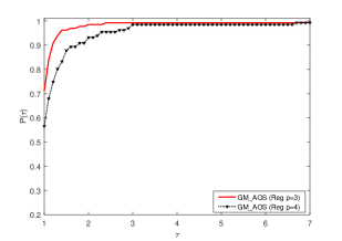
Figure 1: Performance profile based on $N_{iter}$(CUTEr145)

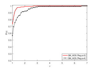
Figure 2: Performance profile based on $N_{f}$(CUTEr145)

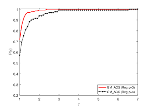
Figure 3: Performance profile based on $N_{g}$(CUTEr145)

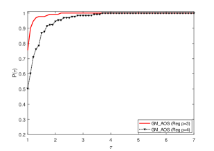
Figure 4: Performance profile based on $T_{cpu}$(CUTEr145)

GM_AOS (1.2)Liu2018Several and the BB method used the same line search as that in GM$\_$AOS (Reg). CGOPT(1.0), CG$\_$DESCENT (5.0) and BBQ used all default settings of parameters but the stopping conditions. Each test method is terminated if ${\left\|{{g_{k}}}\right\|_{\infty}}\leq{10^{-6}}$ or the iterations exceeds 140,000.

The performance profiles introduced by Dolan and Moré25 were used to display the performance of these methods. In the following figures, “$N_{iter}$”, “$N_{f}$”, “$N_{g}$” and “$T_{cpu}$” represent the number of iterations, the number of function evaluations, the number of gradient evaluations and CPU time (s), respectively.

We first compare GM$\_$AOS (Reg p=3) with GM$\_$AOS (Reg p=4) on the test set CUTEr145, and use the better one to compare with other test methods. As shown in Figs. 2-4, we see that GM$\_$AOS (Reg p=3) performs better than GM$\_$AOS (Reg p=4) in term of $N_{iter}$, $N_{f}$, $N_{g}$ and $T_{cpu}$. So we select GM$\_$AOS (Reg p=3) to compare with other test methods in the following numerical experiments.

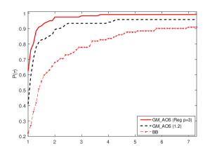
Figure 5: Performance profile based on $N_{iter}$(CUTEr145)

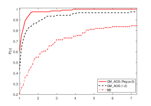
Figure 6: Performance profile based on $N_{f}$(CUTEr145)

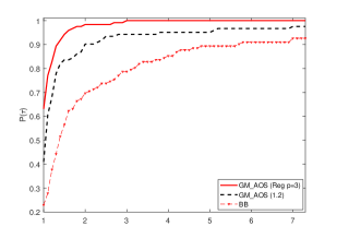
Figure 7: Performance profile based on $N_{g}$(CUTEr145).

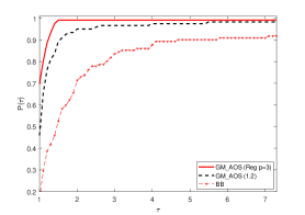
Figure 8: Performance profile based on $T_{cpu}$(CUTEr145).

The following numerical experiments are divided into four groups.

In the first group of the numerical experiments, we compare the performance of GM$\_$AOS (Reg p=3) with that of GM$\_$AOS (1.2) Liu2018Several and the BB method on the test set CUTEr145. Figs. 6-8 present the performance profiles on the test set CUTEr145. As shown in Figs. 6-8, we can observe that GM$\_$AOS (Reg p=3) performs better than GM$\_$AOS (1.2) and is superior much to the BB method, and GM$\_$AOS (1.2) outperforms the BB method. The first group of the numerical experiments indicates that the approximately optimal stepsize is extremely efficient.

In the third group of the numerical experiments, we compare the numerical performance of GM$\_$AOS (Reg p=3) and the BBQ method on the test set CUTEr145. In the numerical experiment, we do not compare the performance about the running time due to the fact that the BBQ method was implemented by Matlab code and GM$\_$AOS (Reg p=3) was implented by C code. As shown in Fig. 10, 10 and 11, we can observed that GM$\_$AOS (Reg p=3) is superior to the BBQ method for the test set CUTEr145 in term of the number of iteration, the number of funciton evaluation and the number of gradient evaluation, while the BBQ method has been regarded as the import advance for gradient method.

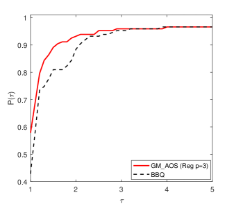
Figure 9: Performance profile based on $N_{iter}$

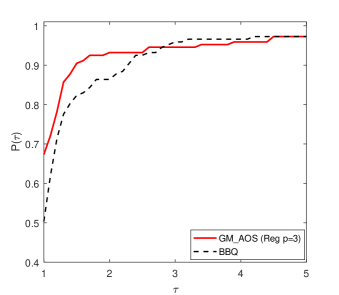
Figure 10: Performance profile based on $N_{f}$

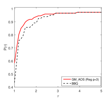
Figure 11: Performance profile based on $N_{g}$

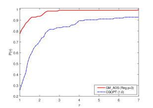
Figure 12: Performance profile based on $N_{f}$(CUTEr145)

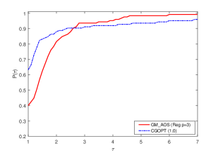
Figure 13: Performance profile based on $N_{g}$(CUTEr145)

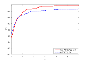
Figure 14: Performance profile based on $N_{f}+3N_{g}$(CUTEr145).

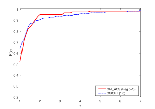
Figure 15: Performance profile based on $T_{cpu}$(CUTEr145).

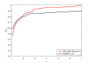
Figure 16: Performance profile based on $N_{iter}$(Andr80)

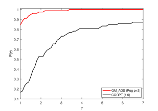
Figure 17: Performance profile based on $N_{f}$(Andr80)

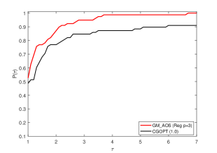
Figure 18: Performance profile based on $N_{g}$(Andr80).

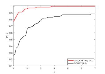
Figure 19: Performance profile based on $T_{cpu}$(Andr80).

In the second group of the numerical experiments, we compare the performance of GM_AOS (Reg p=3) with that of CGOPT (1.0) on the two test sets CUTEr145 and Andr80. Figs. 13-15 present the performance profiles on the test set CUTEr145. As shown in Fig. 13, we see that GM_AOS (Reg p=3) performs much better CGOPT (1.0) in term of $N_{f}$, since GM_AOS (Reg p=3) solves successfully about 79$\%$ test problems with the least function evaluations, while the percentage of CGOPT (1.0) is only about 38$\%$. Fig. 13 indicates that GM_AOS (Reg p=3) is at a disadvantage over CGOPT (1.0) in term of $N_{g}$, and Fig. 15 shows that GM_AOS (Reg p=3) outperforms slightly CGOPT (1.0) in term of $N_{f}+3N_{g}$ HagerLMCGDESCENT . We can observe from Fig. 15 that GM_AOS (Reg p=3) is as fast as CGOPT (1.0). Figs. 17-19 present the performance profiles on the test set Andr80. As shown in Figs. 17-19, we observe that GM_AOS (Reg p=3) illustrates huge advantage over CGOPT (1.0) on the test set Andr80. The second group of the numerical experiments indicates that GM_AOS (Reg p=3) is competitive to CGOPT (1.0) on the test set CUTEr145, and has a significant improvement over CGOPT (1.0) on the test set Andr80.

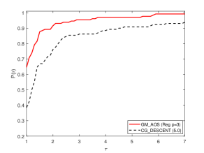
Figure 20: Performance profile based on $N_{f}$(CUTEr145)

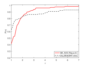
Figure 21: Performance profile based on $N_{g}$(CUTEr145)

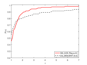
Figure 22: Performance profile based on $N_{f}+3N_{g}$(CUTEr145)

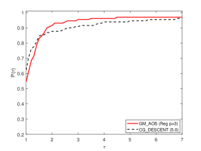
Figure 23: Performance profile based on $T_{cpu}$(CUTEr145)

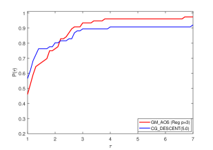
Figure 24: Performance profile based on $N_{iter}$(Andr80)

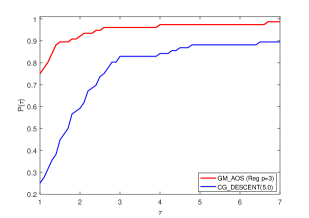
Figure 25: Performance profile based on $N_{f}$(Andr80)

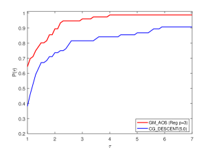
Figure 26: Performance profile based on $N_{g}$(Andr80)

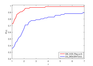
Figure 27: Performance profile based on $T_{cpu}$(Andr80)

In the fourth group of the numerical experiments, we compare the performance of GM_AOS (Reg p=3) with that of CG_DESCENT (5.0) on the two test sets CUTEr145 and Andr80. Figs. 21-23 present the performance profiles on the test set CUTEr145. As shown in Fig. 21, we see that GM_AOS (Reg p=3) performs better than CG_DESCENT (5.0) in term of $N_{f}$, since GM_AOS (Reg p=3) solves successfully about 65$\%$ test problems with the least function evaluations, while the percentage of CG_DESCENT (5.0) is only about 39$\%$. Fig. 21 shows that GM_AOS (Reg p=3) is at a disadvantage over than CG_DESCENT (5.0) in term of $N_{g}$, and Fig. 23 indicates that GM_AOS (Reg p=3) outperforms slightly CG_DESCENT (5.0) in term of $N_{f}+3N_{g}$ HagerLMCGDESCENT . We can observe from Fig. 23 that GM_AOS (Reg p=3) is as fast as CG_DESCENT (5.0). Figs. 25-27 present the performance profiles on the test set Andr80. As shown in Figs. 25-27, we see that GM_AOS (Reg p=3) is at a little disadvantage over CG_DESCENT (5.0) in term of $N_{iter}$, and has a significant performance boost over CG_DESCENT (5.0) in term of $N_{f}$ and $N_{g}$. We also can see that GM_AOS (Reg p=3) is faster much than CG_DESCENT (5.0). The third group of the numerical experiments indicates that GM_AOS (Reg p=3) is competitive to CG_DESCENT (5.0) on the test set CUTEr145, and has a significant improvement over CG_DESCENT (5.0) on the test set Andr80.

Table 1. The number of test problems

Method	$N_{\text{linsear}}=0$	$N_{\text{linsear}}\leq 1$	$N_{\text{linsear}}\leq 2$	$N_{\text{linsear}}\leq 3$	total problems
BB	41	46	48	50	145(CUTEr145)
GM_AOS (Reg p=3)	68	81	85	90	145(CUTEr145)
GM_AOS (Reg p=4)	51	57	60	62	80(Andr80)

As for the reasons for the suprising numerical effect of GM_AOS (Reg p=3), we think that they lie in two aspects: (i)The approximately optimal stepsize is generated by the approximation models including regularization models and quadratic models at the current iterate $x_{k}$, which implies that it is incorporated

properly into more second order or high order information of the objective function. (ii)The approximately optimal stepsize can readily satisfy Zhang-Hager line search directly in most cases compared to other stepsizes in gradient method, which implies that it require less much function evaluations and thus save much computational cost. This can be observed in Figs. 6, 13, 17, 21 and 25. More results can be seen in Table LABEL:table1. In Table LABEL:table1, $N_{\text{linsear}}$ represents the times that the stepsize is updated by (40) during all iterations of solving a test problem, namely, the times that Zhang-Hager line search is invoked during all iterations of solving a test problem. $N_{\text{linsear}}=0$ indicates the initial stepsize (approximately optimal stepsize or BB stepsize) satisfies Zhang-Hager line search (33) directly at all iterations and thus Zhang-Hager line search is not invoked at all. As shown in Table LABEL:table1, we can see that there are 68 (out of 145) problems for which Zhang-Hager line search is not invoked at all during the solving process, while the number for the BB method is only 41, and there are 90 (out of 145) problems for each of which the times that Zhang-Hager line search is invoked is less than or equal to 3, while the number for the BB method is only 50. We also can see that there are 51 (out of 80) problems for which Zhang-Hager line search is not invoked at all during the solving process. Table LABEL:table1 indicates that the approximately optimal stepsize in GM_AOS (Reg p=3) is easier much to meet Zhang-Hager line search (33) directly.

6 Conclusion and discussion

In this paper, we present two efficient gradient methods with approximately optimal stepsize for unconstrained optimization. In the proposed method, some approximation models including regularization models and quadratic models are exploited carefully to derive approximately optimal stepsize. The convergence of the proposed methods is analyzed. Extensive numerical results indicates that the proposed method GM$\_$AOS (Reg p=3) is superior to the BBQ method and other efficient gradient methods, and is competitive to two quite efficient and well-known conjugate gradient software packages CG$\_$DESCENT (5.0) and CGOPT (1.0) on the 145 test problems in the CUTEr library, has significant improvement over CG$\_$DESCENT (5.0) and CGOPT (1.0) on the 80 test problems collected by Andrei. As for the reason that GM$\_$AOS (Reg p=3) has so important improvement over CG$\_$DESCENT (5.0) and CGOPT (1.0) on Andr80 and is only competitive to CG$\_$DESCENT (5.0) and CGOPT (1.0) on CUTEr145, I think that it lies mainly in that most test problems in CUTEr145 is relatively difficult to solve compared to the test problems in Andr80. It seems that one can draw the following conclusion: Gradient methods with approximately optimal stepsize are sufficient for those test problems that are not very ill-conditioned.

Given that the facts: (i)the search direction $-g_{k}$ has low storage; (ii)the approximately optimal stepsize can be easily computed; (iii)the nonmonotone Armijo line search used can be easily implemented; (iv)the numerical effect is surprisingly nice, the gradient methods with approximately optimal stepsizes can become strong candidates for large scale unconstrained optimization and has potential in constrained optimization and some fields such as machine learning.

Though gradient methods with approximately optimal stepsize is surprisingly efficient, there are still some questions under investigation:

(i)Does gradient method with approximately optimal stepsize based on quadratic approximation model (21) possess Q-linear convergence for convex quadratic minimization? If yes, what conditions should be imposed on the distance $\left\|B_{k}-A\right\|$ ? Here $A$ is the Hessian matrix for strictly convex quadratic function.

(ii)It will be an interesting research for combining approximately optimal stepsize wih Cauchy stepsize in convex quadratic minimization. How should one combine approximately optimal stepsize with Cauchy stepsize for obtaining better convergence rate in convex quadratic minimization?

(iii)Can the type of gradient method with approximately optimal stepsize possess local R-linear convergence or better convergence rate when it is applied to general unconstrained optimization?

(iv)There are still a large room for improving numerical performance of gradient methods with approximately optimal stepsizes by exploiting other adaptive appriximation models based on the properties of the objective function.

References

• (1) Cauchy A. Méthode générale pour la résolution des systéms déquations simultanées. Comp. Rend. Sci. Paris. 1847, 25: 46-89.
• (2) Akaike H. On a successive transformation of probability distribution and its application to the analysis of the optimum gradient method. Ann. Inst. Statist. Math. 1959, 11: 1-17.
• (3) Barzilai J., Borwein J. M. Two-point step size gradient methods. IMA J. Numer. Anal. 1988, 8(1): 141-148.
• (4) Raydan M. On the Barzilai and Borwein choice of steplength for the gradient method. IMA J. Numer. Anal. 1993, 13(3): 321-326.
• (5) Dai Y. H., Liao L. Z. R-linear convergence of the Barzilai and Borwein gradient method. IMA J. Numer. Anal. 2002, 22(1): 1-10.
• (6) Li D. W., Sun R. Y. On a faster R-linear convergence rate of the Barzilai-Borwein method. arXiv preprint arXiv: 2101.00205, (2020).
• (7) Dai Y. H., Zhang H. C. An adaptive two-point stepsize gradient algorithm. Numer. Algorithms 2001, 27(4): 377-385.
• (8) Raydan M. The Barzilai and Borwein gradient method for the large scale unconstrained minimization problem. SIAM J. Optim. 1997, 7: 26-33.
• (9) Grippo L., Lamparillo F., Lucidi S. A nonmonotone line search technique for Newton’s method. SIAM J. Numer. Anal. 1986, 23: 707-716.
• (10) Dai Y. H., Yuan J. Y., Yuan Y. X. Modified two-point stepsize gradient methods for unconstrained optimization. Comput. Optim. Appl. 2002. 22(1): 103-109.
• (11) Biglari F., Solimanpur M. Scaling on the spectral gradient method. J. Optim. Theory Appl. 2013, 158(2): 626-635.
• (12) Zhang H. C., Hager W. W. A nonmonotone line search technique and its application to unconstrained optimization. SIAM J. Optim. 2004, 14(4): 1043-1056.
• (13) Liu, Z. X., Liu, H. W., Dong, X. L.: An efficient gradient method with approximate optimal stepsize for the strictly convex quadratic minimization problem. Optimization 2018, 67(3): 427-440.
• (14) Liu Z. X., Liu H. W. An efficient gradient method with approximate optimal stepsize for large-scale unconstrained optimization. Numer. Algorithms 2018, 78(1): 21-39.
• (15) Liu, Z. X., Liu, H. W.: Several efficient gradient methods with approximate optimal stepsizes for large scale unconstrained optimization. J. Comput. Appl. Math. 2018, 328: 400-413.
• (16) Andrei, N.: An unconstrained optimization test functions collection. Adv. Model. Optim. 2008, 10: 147-161.
• (17) Hager W. W., Zhang H. C. A new conjugate gradient method with guaranteed descent and anefficient linesearch. SIAM J. Optim. 2005, 16: 170-192.
• (18) Sun W. Y., Xu. D. A filter-trust-region method based on conic model for unconstrained optimization (in Chinese). Sci. Sin. Math. 2012, 55: 527-543.
• (19) Sun W. Y. Optimization methods for non-quadratic model. Asia-Pac. J. Oper. Res. 1996, 13: 43-63
• (20) Cartis C., Gould N. I., Toint P. L. Adaptive cubic regularisation methods for unconstrained optimization. Part I: motivation, convergence and numerical results. Math. Program. 2011, 127(2): 245-295.
• (21) Cartis C., Gould N. I., Toint P. L. Adaptive cubic regularisation methods for unconstrained optimization. Part II: worst-case function-and derivative-evaluation complexity. Math. Program. 2011, 130(2): 295-319.
• (22) Bianconcini T., Liuzzi G., Morini B. On the use of iterative methods in cubic regularization for unconstrained optimization. Comput. Optim. Appl. 2015, 60(1): 35-57.
• (23) Wei Z. X., Li L., Lu. S. Nonmontone adaptive cubic overestimation methods for unconstrained optimization. J. Guangxi Univ. 2009 34(1): 115-119.
• (24) Toint P L. A non-monotone trust-region algorithm for nonlinear optimization subject to convex constraints. Math. Program. 1997, 77(3): 69-94.
• (25) Bianconcini T., Sciandrone M. Q. A cubic regularization algorithm for unconstrained optimization using line search and nonmonotone techniques. Optim. Methods Softw. 2016, 31: 1008-1035.
• (26) Zhang J. Z., Deng N. Y., Chen L. H. New quasi-Newton equation and related methods for unconstrained optimization. J. Optim. Theory Appl. 1999, 102(1): 147-167.
• (27) Miladinović, M., Stanimirović, P., Miljković, S.: Scalar Correction Method for Solving Large Scale Unconstrained Minimization Problems. J. Optim. Theory Appl. 2011, 151(2): 304-320.
• (28) Birgin E. G., Martínez J. M., Raydan M. Nonmonotone spectral projected gradient methods for convex sets. SIAM J. Optim. 2000, 10: 1196-1211.
• (29) Dolan E. D., Moré J. J. Benchmarking optimization software with performance profiles. Math. Program. 2002, 91: 201-213.
• (30) Dai. Y. H., Hager, W. W., Schittkowski, K., et al.: The cyclic Barzilai-Borwein method for unconstrained optimization. IMA J. Numer. Anal. 2006, 26(3): 604-627.
• (31) Xiao, Y. H., Wang, Q. Y., Wang, D., et al.: Notes on the Dai-Yuan-Yuan modified spectral gradient method. J. Comput. Appl. Math. 2010, 234(10): 2986-2992.
• (32) Nosratipour, H., Fard, O. S., Borzabadi, A. H.: An adaptive nonmonotone global Barzilai-Borwein gradient method for unconstrained optimization. Optimization 2017, 66(4): 641-655.
• (33) Miladinović, M., Stanimirović, P., Miljković, S.: Scalar correction method for solving large scale unconstrained minimization problems. J. Optim. Theory Appl. 2011, 151(2): 304-320.
• (34) Liu, H. W., Liu, Z. X., Dong, X. L.: A new adaptive Barzilai and Borwein method for unconstrained optimization. Optim. Lett. 2018, 12(4): 845-873.
• (35) Gould, N. I. M., Orban, D., Toint, Ph.L.: CUTEr and SifDec: A constrained and unconstrained testing environment, revisited. ACM Trans. Math. Softw. 2003, 29(4): 373-394.
• (36) Dai, Y. H., Kou, C. X.: A nonlinear conjugate gradient algorithm with an optimal property and an improved Wolfe line search. SIAM J. Optim. 2013, 23(1): 296-320.
• (37) Hager, W. W., Zhang, H. C.: A new conjugate gradient method with guaranteed descent and an efficient line search. SIAM J. Optim. 16(1), 2005: 170-192.
• (38) Hager, W. W., Zhang, H. C.: Algorithm 851: CG$\_$DESCENT, a conjugate gradient method with guaranteed descent. ACM Trans. Math. Softw. 2006, 32(1): 113-137.
• (39) Cartis, C., Gould, N. I. M., Toint, P. L.: Adaptive cubic regularisation methods for unconstrained optimization. Part i: motivation, convergence and numerical results. Math. Program. 2011, 127: 245-295.
• (40) Gould, N. I. M., Porcelli, M.: Updating the regularization parameter in the adaptive cubic regularization algorithm. Comput. Optim. Appl. 2012, 53: 1-22.
• (41) Huang Y. K., Dai, Y. H., Liu X. W. Equipping Barzilai-Borwein method with two dimensional quadratic termination property, SIAM Journal on Optimization, 2021,31(4), 3068–3096.
• (42) Yuan Y X. A new stepsize for the steepest descent method, J. Comput. Math., 2006, 24:149-156