Jan Kochanowski University in Kielce
	Faculty of mathematics and natural sciences

Doctoral Thesis
EXACT SOLUTIONS
OF THE RELATIVISTIC
BOLTZMANN EQUATION
IN THE RELAXATION TIME
APPROXIMATION
Ewa Maksymiuk
The thesis prepared in the Institute of Physics
under supervision by prof. dr hab. Wojciech Florkowski
and auxiliary supervision by dr hab. Radosław Ryblewski
Kielce 2018

Abstract

This Thesis concentrates on the analysis of coupled RTA (relaxation time approximation) kinetic equations for bosons and fermions. Bosons are treated as massless particles, while fermions have a finite mass. Using analytic and numerical methods we find exact solutions for such a mixture in the case of one-dimensional, boost-invariant expansion (for systems which are transversally homogeneous). In this way, we generalize several earlier results obtained for one-component systems and classical particles.

Throughout the text, we refer to fermions and bosons as to quarks and gluons, respectively. There are, however, important differences between our particles and real quarks and gluons appearing in the QCD field-theoretic calculations. In particular, we assume that the relaxation times used in the kinetic equations are the same for bosons and fermions. Moreover, the common relaxation time used in the numerical calculations is independent of the momenta of colliding particles and taken to be a constant. Due to such simplifications, our approach cannot be treated as a truly realistic model for QGP. However, it includes most of the important aspects connected with the hydrodynamization and equilibration processes, which are the main topics studied in this work.

Our numerical results illustrate how a non-equilibrium mixture approaches hydrodynamic regime described by the Navier-Stokes equations. We determine appropriate forms of the viscous kinetic coefficients. The shear viscosity of a mixture turns out to be the sum of the shear viscosities of boson and fermion components, while the bulk viscosity is given by the formula derived earlier for a gas of fermions, however, with the thermodynamic coefficients characterizing the whole boson-fermion mixture. Consequently, we find that massless bosons do contribute in a non-trivial way to the bulk viscosity of a mixture (provided quarks are massive).

We further observe the hydrodynamization effect which takes place earlier in the shear sector than in the bulk one — the equalization of the longitudinal and transverse pressures takes place earlier than the equalization of the average and equilibrium pressures. The numerical studies of the ratio of the longitudinal and transverse pressures show that, to a good approximation, it depends on the ratio of the relaxation and evolution times only. We find that this behavior is connected with the existence of an attractor for conformal systems.

Our system of kinetic equations is subsequently used to construct a corresponding scheme of anisotropic hydrodynamics, which can be treated as an effective description of the underlying microscopic dynamics defined by the kinetic model. The comparisons between predictions of anisotropic hydrodynamics and exact solutions of the kinetic equations are used to validate our hydrodynamic approach.

Streszczenie

Niniejsza praca koncentruje się na analizie sprzężonych równań kinetycznych w tzw. przybliżeniu czasu relaksacji, opisujących mieszaninę bozonów i fermionów, przy czym bozony traktowane są jako cząstki bezmasowe, zaś fermiony posiadają skończoną masę. Użycie metod analitycznych i numerycznych umożliwia znalezienie dokładnych rozwiązań w przypadku takiej mieszaniny, podlegającej jednowymiarowej i boost-niezmienniczej ekspansji. Tym samym uogólnione zostały poprzednie wyniki, uzyskane dla układów składających się z cząstek jednego rodzaju, rządzonych statystyką klasyczną.

W całej pracy przez fermiony rozumie się kwarkami (oznaczone symbolem $Q$), zaś bozony nazywamy gluonami (oznaczone symbolem $G$). Należy jednak zwrócić uwagę na istotną różnicę pomiędzy cząstkami dyskutowanymi w pracy, a rzeczywistymi kwarkami i gluonami, pojawiającymi się w teoretycznych rachunkach QCD. Niniejsze rozwiązania opierają się na założeniu, że czasy relaksacji użyte w równaniu kinetycznym są takie same dla bozonów i fermionów. Co więcej, czas relaksacji używany w rachunkach numerycznych jest niezależny od pędu zderzających się cząstek i został przyjęty jako stały. W związku z tymi uproszczeniami, prezentowane podejście nie może być traktowane jako bardzo realistyczny model plazmy kwarkowo-gluonowej. Nie zmienia to jednak faktu, że niniejszy opis zawiera wiekszość ważnych aspektów związanych z procesami hydrodynamizacji i osią-gania równowagi, bądącymi najważniejszymi tematami poruszanymi w pracy.

Numeryczne rezultaty ilustrują w jaki sposób nierównowagowa mieszanina cząstek osiąga hydrodynamiczny obszar opisywany przez równania Naviera-Stokesa. Wyznaczone zostały odpowiednie formy współczynników kinetycznych. Lepkość dynamiczna mieszaniny (ang. shear viscosity) okazała się być sumą lepkości dynamicznych bozonów i fermionów. Z kolei w przypadku lepkości objętościowej (ang. bulk viscosity), danej przez formułę wyprowadzoną wcześniej dla gazu fermionów okazało się, że należy uwzględniać współczynniki termodynamiczne, charakteryzujące całą mieszaninę bozonów i fermionów. Tym samym bezmasowe bozony przyczyniają się w nietrywialny sposób do lepkości objętościowej.

W dalszej kolejności zaobserwowaliśmy efekty hydrodynamizacji, które następują wcześniej w sektorze dynamicznym niż objętościowym — wyrównanie się ciśnień podłuż-nego i poprzecznego ma miejsce wcześniej niż wyrównanie się ciśnienia średniego i równowa-gowego. Analiza numeryczna stosunku ciśniena podłużnego do poprzecznego pokazuje z bardzo dobrą dokładnością zależność jedynie od stosunku czasu relaksacji i czasu własnego ewolucji. Zachowanie to jest związane z istnieniem atraktora dla układów konforemnych.

Dyskutowany układ równań kinetycznych jest następnie użyty do konstrukcji odpowiedniego układu równań hydrodynamiki anizotropowej, która może być traktowana jako efektywny opis zasadniczej dynamiki mikroskopowej, definiowanej przez model kinetycz-ny. Porównania pomiędzy przewidywaniami hydrodynamiki anizotropowej i dokładnych rozwiązań równań kinetycznych są użyte do pozytywnego zweryfikowania naszego podejścia hydrodynamicznego.

I would like to thank and express the deepest gratitude and appreciation to my supervisor, Wojciech Florkowski, and to my co-supervisor, Radosław Ryblewski, for introducing me to the extremely interesting and beautiful branch of heavy ion physics, and for giving me an opportunity to work in very friendly atmosphere during my research.

My final thanks are directed for my beloved Michał, my sister Monika, my Parents, and all of my friends for their huge support.

RHIC	Relativistic Heavy-Ion Collider at Brookhaven National Laboratory
LHC	Large Hadron Collider at CERN
QCD	quantum chromodynamics
QGP	quark-gluon plasma
wQGP	weakly coupled QGP
sQGP	strongly coupled QGP
IS	Israel-Stewart (hydrodynamic equations)
NS	Navier-Stokes (hydrodynamic equations)
KT	kinetic theory
aHydro	anisotropic hydrodynamics
RTA	relaxation time approximation
RS	Romatschke-Strickland (ansatz for the distribution function)
EOS	equation of state
eq	label specifying local thermal equilibrium

Table 1: List of acronyms

$T^{\mu\nu\,{\rm}}$	energy-momentum tensor
$T$	effective temperature
$\mu$	effective chemical potential
$U^{\mu}$	flow vector defining the Landau hydrodynamic frame
$\Delta^{\mu\nu}$	operator projecting on the space orthogonal to $U^{\mu}$
$\Pi$	bulk pressure
${\cal E}$	energy density
${\cal S}$	entropy density
${\cal B}$	baryon number density
${\cal P}_{\rm eq}({\cal E})$	equilibrium pressure corresponding to the energy density ${\cal E}$
	(functional form ${\cal P}_{\rm eq}({\cal E})$ follows from the equation of state)
$\eta$	shear viscosity
$\zeta$	bulk viscosity
${\bar{\eta}}=\eta/{\cal S}$	ratio of shear viscosity and entropy density

Table 2: Symbols denoting physical concepts and variables

spacetime variables
$g_{\mu\nu}={\rm diag}(1,-1,-1,-1)$	metric tensor
$x^{\mu}=(x^{0},x^{1},x^{2},x^{3})=(t,x,y,z)$	space-time coordinates
$r=\sqrt{x^{2}+y^{2}}$	distance from the collision axis
$\phi=\arctan(y/x)$	azimuthal angle
$\theta=\arctan(r/z)$	polar angle
$\tau=\sqrt{t^{2}-z^{2}}$	proper (longitudinal) time
$\eta=\frac{1}{2}\ln\frac{t+z}{t-z}$	spacetime rapidity
$U^{\mu},X^{\mu},Y^{\mu},Z^{\mu}$	basis four-vectors
kinematical variables
describing a single particle
$p^{\mu}=(p^{0},p^{1},p^{2},p^{3})=(E_{p},p_{x},p_{y},p_{z})$	four-momentum
$p^{0}=p_{0}=E_{p}$	energy
$E_{p}=\sqrt{m^{2}+p^{2}}$	mass-shell energy
$p^{3}=-p_{3}=p_{z}=p_{L}$	longitudinal momentum of a particle
$p_{T}=\sqrt{p_{x}^{2}+p_{y}^{2}}$	transverse momentum of a particle
$\phi_{p}=\arctan(p_{y}/p_{x})$	momentum azimuthal angle

Table 3: Symbols of the physical quantities related to space, time, and momenta of particles.

anisotropic
energy-momentum tensors
$T^{\mu\nu}_{\rm a}$	leading-order energy-momentum tensor for aHydro
${\cal P}_{T}^{\rm a}$	transverse pressure
${\cal P}_{L}^{\rm a}$	longitudinal pressure
parameters of anisotropic
distribution functions
$\xi_{Q}$	anisotropy parameter for quarks
$\xi_{G}$	anisotropy parameter for gluons
$\Lambda_{Q}$	transverse-momentum scale for quarks
$\Lambda_{G}$	transverse-momentum scale for gluons
$\lambda$	the non-equilibrium chemical potential for quarks

Table 4: Symbols and concepts used in aHydro

Chapter 1 Introduction

1.1 Ultra-relativistic heavy-ion collisions
and quark-gluon plasma

The topics discussed in this Thesis belong to a broad physics field of ultra-relativistic heavy-ion collisions [1, 2, 3, 4, 5, 6, 7, 8, 9, 10, 11, 12, 13, 14, 15, 16, 17, 18]. This type of research combines the methods of high-energy physics of elementary particles with nuclear physics. However, a characteristic feature of heavy-ion collisions is that systems consisting of a large number of particles are produced in such processes, hence, theoretical tools based on the use of thermodynamics, statistical physics, hydrodynamics and/or kinetic theory concepts are commonly used to interpret the experimental results.

One of the conclusions of the experimental programs performed at RHIC ​ and the LHC is that relatively simple thermodynamic and/or hydrodynamic models are indeed quite successful in a description of the data [19, 20, 21, 22, 23]. This, in turn, leads to new questions about the applicability range of such methods. One of the persistent problems discussed in the context of heavy-ion collisions is why the particle abundances and spectra have thermal features. Is there enough time for such microscopic processes so that they can lead to a thermalized state? Another problem is applicability of hydrodynamics. Are the gradients of local hydrodynamic variables sufficiently small that hydrodynamics becomes a suitable framework for the determination of space-time evolution of the produced matter?

In the last years, at least partial answers to the questions mentioned above have been found. It seems that the timescales involved in heavy-ion collisions are sufficiently long so that the produced matter may emerge locally equilibrated at freeze-out. On the other hand, there is a growing evidence that hydrodynamics (at least in its modern formulations) may be applied in the situations where systems are far away from local equilibrium. In this way, relativistic hydrodynamics becomes a theoretical tool connecting early, non-equilibrium stages with the late, locally equilibrated system configurations.

One way of introducing the equations of relativistic hydrodynamics is that one starts from the underlying kinetic theory and derives the hydrodynamic equations by taking a specific set of the moments of the kinetic equation. In this case, the efficacy of the hydrodynamic approach can be verified by the comparisons of hydrodynamic predictions with the kinetic-theory results. Such methodology has been successfully used in the past [24, 25], and our present work contributes to this type of studies: herein we report in detail on the new exact solutions of the Boltzmann equation and compare our kinetic-theory results with the outcome of anisotropic hydrodynamics [26, 27] which represents one of the new hydrodynamic frameworks.

1.1.1 Searches for new phases of strongly interacting matter

The ultimate aim of the physics of ultra-relativistic heavy-ion collisions is the observation of new states of matter predicted by quantum chromodynamics (QCD) and by model calculations inspired by QCD. In fact, the experimental results collected at RHIC are treated now as the evidence for production of a strongly coupled quark-gluon plasma (sQGP) in the analyzed collisions. One source of this evidence is a very successful use of the viscous hydrodynamics to describe the data. Relativistic viscous hydrodynamics forms the basic ingredient of the models describing heavy-ion collisions at the top RHIC energies. It turns out that a small ratio of the shear viscosity $\eta$ to the entropy density ${\cal S}$ is required to reproduce well the data.  The smallness of the shear viscosity signals the presence of a strongly coupled fluid. Another signal of a strongly coupled system is the phenomenon of jet quenching.

We note that in heavy-ion collisions we deal with systems of quarks and gluons that always interact strongly, i.e., their fundamental interaction theory is QCD. However, because of the running of the QCD coupling constant, the interaction strength can have a different magnitude. By a strongly coupled QGP, we understand the quark-gluon system with an effective large coupling constant. As the matter of fact, one sometimes argues that the very concept of particles may be not adequate for such a system. On the other hand, by a weakly coupled quark-gluon plasma (wQGP) we mean an asymptotic state where the coupling constant is small. In the next two sections, we describe how the concepts of the quark-gluon plasma evolved in time.

1.1.2 Perturbative concept of quark-gluon plasma

Originally, the concepts of the quark-gluon plasma referred only to a weakly coupled plasma. The idea of formation of such a state in heavy-ion collisions was motivated by the phenomenon of the asymptotic freedom in QCD — densely packed quarks and gluons should interact weakly and form a kind of gas of particles with color charges. The name “quark-gluon plasma” was introduced by Shuryak in 1978 [29, 30].

The weakly coupled QGP has (in the leading order of the coupling) simple thermodynamic properties which follow directly from expressions for the Bose-Einstein (gluons) and Fermi-Dirac (quarks) gases. It has more effective degrees of freedom than a hadron gas and one expects the occurrence of a phase transition between the hadron gas and QGP as the system’s temperature and/or density increases.

The first heavy-ion experiments with relativistic beams were aiming at the creation of such an asymptotic QGP state. Several so-called QGP plasma signatures were proposed as the manifestation of the plasma formation (they included, for example, the phenomena of enhanced strangeness production [31] and $J/\psi$ suppression [32]). Although the physics interpretation of those signatures was not always quite straightforward, taken together, they motivated the physicists from CERN to announce in the year 2000 that a new state of matter was found[33].

1.1.3 Strongly coupled quark-gluon plasma

The experimental data coming from the RHIC experiments (which started, by the way, just after the CERN statement of 2000), together with their theoretical explanations, changed the paradigm of a weakly coupled QGP. This was possible due to an enormous progress made in both the experimental techniques (which delivered new high-quality data) and theoretical tools and models (which allowed for a quantitative description of the measurements). As we have mentioned above, the smallness of shear viscosity and the phenomenon of jet quenching observed at RHIC pointed out to a strongly-coupled character of QGP. Recent results from the LHC seem to confirm these findings suggesting that the beam energies available at the moment in the colliders are insufficient to reach the regime of a weakly-coupled plasma.

The fact that QGP behaves as a strongly coupled fluid has made possible application of the theoretical techniques designed to deal with such systems. In particular, several features of QGP have been explained in the framework of the so-called AdS/CFT correspondence [34, 35]. This approach explains, for example, the small value of the ratio of the shear viscosity to the entropy density, ${\bar{\eta}}=\eta/{\cal S}=1/(4\pi)$ [36] .

Although the AdS/CFT correspondence is suitable for the description of conformal systems rather than of QCD (where conformal symmetry is broken by the renormalization scale and the finite quark masses), its appealing feature is that it delivers exact solutions describing the time dynamics of strongly-coupled non-equilibrium systems. This allows for precise studies of physical systems that approach the hydrodynamic regime.

The use of the AdS/CFT correspondence is frequently confronted with the applications of the kinetic theory since the latter is regarded as an appropriate framework to describe weakly coupled systems. Nevertheless, both AdS/CFT and kinetic theory offer a possibility of analyzing the exact non-equilibrium dynamics. This makes the two approaches equally attractive to study the hydrodynamization and equilibration processes.

1.2 Hydrodynamic description of heavy-ion collisions

1.2.1 Standard model of heavy-ion collisions

Nowadays, one speaks very often about the standard model of heavy-ion collisions (for a recent review see, for example, Ref. [38]). According to this model, the space-time evolution of matter created in heavy-ion collisions can be separated into three different stages. The first stage is highly out of equilibrium and includes the hydrodynamization process which is understood as the approach to the physical regime where dynamics is well described by a viscous relativistic hydrodynamics. The second stage is fully described by hydrodynamics and includes the phase transition from the quark-gluon plasma to a hadron gas. This stage describes local equilibration of the system and ends when the interactions between hadrons become sufficiently weak, so the system enters the (third) stage called freeze-out [39]. The name “freeze-out” denotes freezing of the hadron momenta — noninteracting hadrons have momenta that no longer change in time. The process of freeze-out is commonly divided into at least two subprocesses: the chemical and thermal freeze-outs. The thermal or kinetic freeze-out corresponds to a genuine freeze-out process defined above. On the other hand, the chemical freeze-out corresponds to a transition where inelastic collisions between hadrons cease. The chemical freeze-out (when inelastic processes stop) precedes the thermal freeze-out (when both inelastic and elastic processes stop) .

It is worth mentioning that the standard model defined in this way has a block structure with elements that can be separately exchanged and/or modified. For example, the middle hydrodynamic stage can be described with different hydrodynamics frameworks. Earlier approaches based on the use of the perfect-fluid hydrodynamics are now replaced by sophisticated viscous-hydrodynamics codes.

In this work, we concentrate on the first stage of heavy-ion collisions where the produced matter is out of local thermodynamic equilibrium. Using the framework of the kinetic theory, we can analyze how the analyzed system approaches the regime described by viscous hydrodynamic equations. Certainly, our approach is very simplistic and cannot be treated as a realistic modeling of the early stages. Nevertheless, it contains all important features of non-equilibrium dynamics, allows for finding exact solutions, and can be used to study the phenomenon of hydrodynamization.

1.2.2 From perfect-fluid to the viscous hydrodynamic framework

Perfect-fluid hydrodynamics

Relativistic perfect fluid dynamics provides us with the simplest relativistic fluid dynamical equations[41, 42, 43, 44, 1, 12, 45, 46, 47, 48, 49]. The concept of viscous hydrodynamics is usually connected with an idea of gradient (hydrodynamic) expansion of the energy-momentum tensor [21]. The leading order of hydrodynamic expansion is identified with the perfect-fluid framework, where the gradients are absent and the whole theory follows from the perfect-fluid form of the energy-momentum tensor valid in local equilibrium,

$$T^{\mu\nu}_{\rm eq}=\left({\cal E}+{\cal P}_{\rm eq}\right)U^{\mu}U^{\nu}-g^{\mu\nu}{\cal P}_{\rm eq},$$ (1.1)

and the conservation laws for energy and momentum,

$$\partial_{\mu}T^{\mu\nu}_{\rm eq}=0.$$ (1.2)

Here ${\cal E}$ is the energy density and ${\cal P}_{\rm eq}$ is the equilibrium pressure corresponding to the energy density ${\cal E}_{\rm eq}={\cal E}$ . For systems with finite baryon number, Eqs. (1.1) and (1.2) should be supplemented by the conservation of the baryon number current

$$\partial_{\mu}({\cal B}\,U^{\mu})=0.$$ (1.3)

At this level, the main dynamic variables (hydrodynamic fields) are the local temperature $T(x)$ and three independent components of the flow four-vector $U^{\mu}(x)$, as well as the chemical potential $\mu(x)$ for systems containing a conserved charge such as the baryon number.

Navier-Stokes hydrodynamics

The inclusion of dissipative terms leads to a modification of the energy-momentum tensor (1.1) that can be written in the form

$$T^{\mu\nu}=T^{\mu\nu}_{\rm eq}+\pi^{\mu\nu}+\Pi\Delta^{\mu\nu}.$$ (1.4)

Here $\pi^{\mu\nu}$ is the shear stress tensor, $\Pi$ is the bulk pressure, and $\Delta^{\mu\nu}=g^{\mu\nu}-U^{\mu}U^{\nu}$ is the operator projecting vectors on the space perpendicular to $U$. Choosing the Landau hydrodynamic frame, where

$$T^{\mu\nu}U_{\nu}={\cal E}U^{\mu},$$ (1.5)

we demand that $\pi^{\mu\nu}U_{\nu}=0$. Moreover, the shear stress tensor should be symmetric and traceless (as the effects of the trace are included in the isotropic part related to the bulk pressure). This leaves five independent components in $\pi^{\mu\nu}$. These together with a one degree of freedom represented by $\Pi$ define six additional components of the symmetric energy-momentum tensor (in addition to $T$ and three independent components of $U^{\mu}$).

By including terms linear in gradients of $T$ and $U^{\mu}$, we obtain the Navier-Stokes theory where

$$\pi^{\mu\nu}=2\eta\sigma^{\mu\nu},\qquad\Pi=-\zeta\partial_{\mu}U^{\mu}.$$ (1.6)

Here $\eta$ and $\zeta$ are the shear and bulk viscosity coefficients, respectively, and $\sigma^{\mu\nu}$ is the shear flow tensor. The latter is defined through the expression

$$\sigma^{\mu\nu}=\Delta^{\mu\nu}_{\alpha\beta}\partial^{\alpha}U^{\beta},$$ (1.7)

where the projection operator $\Delta^{\mu\nu}_{\alpha\beta}$ has the form

$$\Delta^{\mu\nu}_{\alpha\beta}=\frac{1}{2}\left(\Delta^{\mu}_{\,\,\,\alpha}\Delta^{\nu}_{\,\,\,\beta}+\Delta^{\mu}_{\,\,\,\beta}\Delta^{\nu}_{\,\,\,\alpha}\right)-\frac{1}{3}\Delta^{\mu\nu}\Delta_{\alpha\beta}.$$ (1.8)

We note that the shear flow tensor is symmetric, orthogonal to $U^{\mu}$, and traceless. Hence, in the Navier-Stokes theory, these properties become immediately the properties of the shear stress tensor, due to the first relation in Eq. (1.6).

Israel-Stewart hydrodynamics

It turns out that the use of the form (1.4) with (1.6) directly in the conservation law (1.2) leads to instabilities and acausal behavior [50]. To remedy this situation, Israel and Stewart modified the hydrodynamic approach [51, 52] by upgrading both $\pi^{\mu\nu}$ and $\Pi$ to new independent hydrodynamic variables that satisfy the following equations

$$\dot{\pi}^{\langle\mu\nu\rangle}+\frac{\pi^{\mu\nu}}{\tau_{\pi}} = \beta_{\pi}\sigma^{\mu\nu},\qquad\tau_{\pi}\beta_{\pi}=2\eta,$$ (1.9)

$$\dot{\Pi}+\frac{\Pi}{\tau_{\Pi}} = -\beta_{\Pi}\partial_{\mu}U^{\mu},\qquad\tau_{\Pi}\beta_{\Pi}=\zeta.$$ (1.10)

The dot denotes here the convective derivative, $U^{\mu}\partial_{\mu}$, while the angular brackets denote contraction with the projector (1.8) (after the calculation of the derivative). The parameters $\tau_{\pi}$ and $\tau_{\Pi}$ are known as the relaxation times for viscous shear stress and bulk pressure, respectively. The coefficients $\beta_{\pi}$ and $\beta_{\Pi}$ are kinetic coefficients that relate the relaxation times with the viscosity coefficients, as described by the right-hand sides of (1.9) and (1.10).

Equations (1.9) and (1.10) are the simplest version of the hydrodynamic equations of the Israel-Stewart type. Nevertheless, they describe the main idea of treating dissipative terms as additional hydrodynamic variables. In practical calculations, one includes more terms on the right-hand sides of (1.9) and (1.10). Their appearance is controlled essentially by the powers of gradients. The shear stress tensor and the bulk pressure are treated, due to Eq. (1.6), as first-order terms. Hence, their derivatives are of the second order in gradients. Consequently, if we want to construct a second-order hydrodynamic theory, the right-hand sides of (1.9) and (1.10) should contain additional terms that are properly constructed products of $\pi^{\mu\nu}$ or $\Pi$ with $\sigma^{\mu\nu}$ or $\partial_{\mu}U^{\mu}$ [53, 54, 55, 56, 57, 58].

The hydrodynamic codes based on the Israel-Stewart approach are the most popular tools to model the expansion of matter produced in heavy-ion collisions. Our estimates of the magnitude of the shear and bulk viscosity follow mainly from such type of calculations.

New developments

One expects usually that $\pi^{\mu\nu}$ and $\Pi$ are small compared to the leading order (perfect-fluid) expressions. However, it turns out that the gradients present at the early stages of heavy-ion collisions are very large and, consequently, the gradient corrections become quite substantial. This observation has produced doubts if the standard viscous hydrodynamics is indeed a reliable tool for the description of heavy-ion collisions. This, in turn, initiated broad analyses of the hydrodynamic concepts, which brought very intriguing answers. One of the new points in this kind of studies is the observation that the early time dynamics of systems is determined by the existence of attractors which “lead the system” towards a hydrodynamic, Navier-Stokes regime [59]. This would correspond to the hydrodynamization process. On the other hand, a subsequent viscous evolution leads the system towards local equilibrium, thus, it is responsible for the process commonly known as thermalization.

1.2.3 Anisotropic hydrodynamics

The problem of “large gradient corrections” motivated also the construction of new hydrodynamic schemes that do not refer to the concept of gradient expansion. In 2010 two groups formulated independently the idea of anisotropic hydrodynamics (aHydro) [26, 27], what was the inspiration for the next important papers [60, 61, 62, 63, 64, 65, 66, 67, 68, 69, 70, 71, 72, 73, 74, 75, 76, 77, 78, 79, 80, 81, 82, 83]. This approach makes use of the kinetic-theory concepts and assumes that the phase-space distribution functions are highly anisotropic. Using simple parametrizations of such functions (in terms of the original or generalized Romatschke-Strickland form [84]) in the RTA kinetic equation, and taking appropriate moments of this equation, one can derive a hydrodynamic framework allowing for the description of systems far away from local equilibrium. The parameters defining anisotropic distributions play a role of hydrodynamic variables. For systems being close to local equilibrium, they can be connected with the shear stress tensor and the bulk pressure.

In constructing the framework of anisotropic hydrodynamics it is not completely obvious which moments of the kinetic equation should be taken into account (except for those leading directly to the conservation laws for energy, momentum, and baryon number). One way to solve this problem is to make comparisons of anisotropic-hydrodynamics predictions with the kinetic-theory results. This approach turned out to be very successful in the past for simple systems [24, 25, 85, 86]. In this work, we use this method to introduce and validate aHydro equations for mixtures. We emphasize that to do such comparisons we have to know exact solutions of the kinetic equation since this allows us for making precise comparisons.

1.3 Kinetic theory

Kinetic (or transport) theory is based on the Boltzmann kinetic equation that is usually very difficult to deal with, as it contains a complicated collision term. The latter accounts for the collisions between particles and has the form of a multidimensional integral. The standard treatment of the Boltzmann equation is that one makes involved numerical simulations describing the free motion of particles as well as their collisions.

Because of this technical difficulties, one quite often uses a simplified version of the kinetic equation with a simplified form of the collision term. This is known in the literature as the relaxation-time approximation (RTA) [87, 88, 89, 90]. The details of this approach will be given below. Here, we only state that the present Thesis is entirely based on this approximation, as it allows for finding exact solutions of the kinetic equation. Similarly to earlier works we also restrict ourselves to boost invariant systems [91, 92], as this is another important assumption that allows for the exact treatment of the dynamics.

For the sake of simplicity, we also assume that the relaxation time is constant and the same for different particles forming the interacting system. The use of a temperature dependent relaxation time, which is a natural choice for conformal theories, increases substantially the computational time but, otherwise, does not introduce any important restrictions for the performed calculations.

We usually consider below the systems consisting of two types of particles: massive fermions and massless bosons. We continue to call them quarks and gluons but it should be emphasized that due to the simplistic character of our kinetic model they differ in many respects from real (perturbative) quarks and gluons.

1.4 Specific aim of this work

A specific aim of this Thesis is to collect, summarize, and update several previous results on the exact solutions of the Boltzmann RTA equation and to clarify their relations to anisotropic hydrodynamics. These results were obtained by the author of this Thesis and collaborators, and have been already published in the following publications:

• W. Florkowski, E. Maksymiuk, R. Ryblewski, and M. Strickland, Exact solution of the (0+1)-dimensional Boltzmann equation for a massive gas, Phys. Rev. C89 (2014) 054908 [93].

• W. Florkowski and E. Maksymiuk, Exact solution of the (0+1)-dimensional Boltzmann equation for massive Bose-Einstein and Fermi-Dirac gases, J. Phys. G42 (2015) 045106 [94].

• W. Florkowski, E. Maksymiuk, R. Ryblewski, and L. Tinti, Anisotropic hydrodynamics for a mixture of quark and gluon fluids, Phys. Rev. C92 (2015) 054912 [95].

• W. Florkowski, E. Maksymiuk, and R. Ryblewski, Coupled kinetic equations for fermions and bosons in the relaxation-time approximation, Phys. Rev. C97 (2018) 024915 [96].

• W. Florkowski, E. Maksymiuk, and R. Ryblewski, Anisotropic-hydrodynamics approach to a quark-gluon fluid mixture, Phys. Rev. C97 (2018) 014904 [97].

• E. Maksymiuk, Exact solutions of the (0+1)-dimensional kinetic equation in the relaxation time approximation, J.Phys.Conf.Ser. 612 (2015) no.1, 012054.
  Conference: Hot Quarks 2014, Las Negras, Spain.

• E. Maksymiuk, Mixture of quark and gluon fluids described in terms of anisotropic hydrodynamics, Acta Phys.Polon.Supp. 10 (2017) 1171 (2017).
  Conference: 9th International Winter Workshop "Excited QCD" 2017, Sintra, Portugal.

• E. Maksymiuk, Kinetic equations and anisotropic hydrodynamics for quark and gluon fluids, EPJ Web Conf. 18 (2018) 20207.
  Conference: 6th International Conference on New Frontiers in Physics (ICNFP 2017), Crete, Greece.

The papers 1, 2 and 4 generalize the results obtained in Refs. [24, 25] to the case of massive particles that obey quantum statistics. The article 5 extends the previous results to the case of a mixture of massive fermions and massless bosons. The papers 3 and 5 construct a framework of anisotropic hydrodynamics for a mixture. The present work is dominantly based on 4 and 5.

The papers 6, 7 and 8 are conference proceedings.

1.5 Summary of the main results

• Using analytic and numerical methods we have found exact solutions of the coupled RTA kinetic equations for massless gluons and massive quarks. In this way we have generalized several previous results obtained for simple (one-component) systems, where particles usually obeyed classical statistics.

• The shear and bulk viscosities of a quark-gluon mixture have been found. It turns out that the shear viscosity $\eta$ is simply a sum of the quark and gluon shear viscosities, $\eta=\eta_{Q}+\eta_{G}$. On the other hand, the bulk viscosity of a mixture is given by the formula known for a massive quark gas, $\zeta$. Nevertheless, we find that $\zeta$ depends on thermodynamic coefficients characterizing the whole mixture rather than quarks alone, which means that massless gluons contribute in a non-trivial way to the bulk viscosity (provided the quarks are massive).

• We find that the hydrodynamization effect takes place earlier in the shear sector than in the bulk one — the equalization of the longitudinal, ${\cal P}_{L}$, and transverse, ${\cal P}_{T}$, pressures takes place earlier than the equalization of the average and equilibrium pressures.

• Our studies of the time evolution of the ratio of the longitudinal and transverse pressures indicate that, to a very good approximation, it depends on the ratio of the relaxation and evolution times only. This behavior is related to the presence of an attractor which was found and discussed earlier for conformal systems [59, 98, 99, 100, 101, 102].

• The results collected in this work confirm that aHydro is a very good approximation for the kinetic-theory results. We find that starting from the different initial condition aHydro reproduces very well the time dependence of several physical quantities, in particular, of the ratio of the longitudinal and transverse pressures. This brings further arguments in favor of using the framework of aHydro for phenomenological modeling of heavy-ion collisions.

1.6 Notation and units

In this section, we define our symbols for four-momenta of particles, space-time coordinates and units, see also Table 3.

1.6.1 Four-momentum parametrization

Due to ultra-relativistic speeds along the $z$-axis, the particle four-momentum is most often parametrized in the following way

$$p^{\mu} = \left(p^{0},p^{1},p^{2},p^{3}\right)=\left(E_{p},p_{x},p_{y},p_{z}\equiv p_{L}\right)$$ (1.11)

$$= \left(m_{T}\cosh y,\,\,p_{T}\!\cos\phi_{p},\,\,p_{T}\!\sin\phi_{p},\,\,m_{T}\sinh y\right),$$

where

$$m_{T}=\sqrt{m^{2}+p_{T}^{2}}$$ (1.12)

is the transverse mass, $p_{T}=\sqrt{p_{x}^{2}+p_{y}^{2}}$ is the transverse momentum,

$$y=\frac{1}{2}\ln\frac{E_{p}+p_{L}}{E_{p}-p_{L}}$$ (1.13)

is the longitudinal rapidity, and

$$\phi_{p}=\tan^{-1}\left(\frac{p_{y}}{p_{x}}\right)$$ (1.14)

is the azimuthal angle in the transverse plane. Due to the on-shell condition, $p^{2}=p^{\mu}p_{\mu}=m^{2}$, only three momentum variables, say, $p_{x}$, $p_{y}$ and $p_{z}$ (or, equivalently, $p_{T}$, $\phi_{p}$ and $y$) are treated as independent which for the momentum covariant integration measure implies

$$\int dP(\dots)=2\int d^{4}p\,\Theta(p^{0})\delta(p^{2}-m^{2})(\dots)=\int\frac{d^{3}p}{E_{p}}(\dots),$$ (1.15)

where $\Theta$ is the Heaviside step function.

1.6.2 Spacetime parametrization

In an analogous way, we parameterize the space-time coordinates 

$$x^{\mu} = \left(x^{0},x^{1},x^{2},x^{3}\right)=\left(t,x,y,z\right)$$ (1.16)

$$= \left(\tau\cosh\eta,r\cos\phi,r\sin\phi,\tau\sinh\eta\right),$$

where $\tau$ is the invariant time (often called the longitudinal proper time)

$$\tau=\sqrt{t^{2}-z^{2}},$$ (1.17)

and $\eta$ is the spacetime rapidity

$$\eta=\frac{1}{2}\ln\frac{t+z}{t-z}.$$ (1.18)

We further define the distance in the transverse plane $r$ and the angle $\phi$ through the equations

$$r=\sqrt{x^{2}+y^{2}},\quad\phi=\tan^{-1}\left(\frac{y}{x}\right).$$ (1.19)

For convenience, we use the following notation for the scalar product: $a\cdot b=a_{\mu}b^{\mu}=g_{\mu\nu}a^{\mu}b^{\nu}$ with the flat-space metric tensor

$$g^{\mu\nu}=\left(\begin{array}[]{cccc}1&0&0&0\\ 0&-1&0&0\\ 0&0&-1&0\\ 0&0&0&-1\end{array}\right),$$ (1.20)

satisfying $g^{\mu\nu}g_{\mu\nu}=4$.

1.6.3 Units

Throughout the text we use natural units with $c=\hbar=k_{B}=1$.

1.7 Text organization

The Thesis is organized as follows: In Chapt. 2 we introduce the system of kinetic equations and study their moments. This leads to two Landau matching conditions related to the baryon number and energy-momentum conservations. The form of the exact solutions of the kinetic equations is discussed in Chapt. 3. Numerical results for various physics observables, obtained with the exact solutions, are presented in Chapt. 4. The concept of anisotropic hydrodynamics is introduced in Chapt. 5. Numerical comparisons of the results obtained with aHydro and kinetic theory are presented in Chapt. 6. We conclude and summarize in Chapt. 7.

Chapter 2 Kinetic equations

2.1 Relaxation time approximation

In this Thesis, we analyze three coupled relativistic Boltzmann kinetic equations for quark (${Q^{+}}$), antiquark (${Q^{-}}$), and gluon (${G}$) phase-space distribution functions $f_{{\rm s}}(x,p)$  [103, 104, 105, 95],

$$p^{\mu}\partial_{\mu}\,f_{{\rm s}}(x,p) = {\cal C}\left[f_{{\rm s}}(x,p)\right],\quad{\rm s}={Q^{+}},{Q^{-}},{G}.$$ (2.1)

The left-hand sides of Eqs. (2.1) describe free motion of particles (they are often dubbed the drift or free-streaming terms), while the right-hand sides contain the collision terms ${\cal C}[f_{{\rm s}}(x,p)]$, which account for interactions in the system. In this work, the latter are included in the relaxation time approximation (RTA) [87, 88, 89], namely, we use the form

$${\cal C}\left[f_{\rm s}(x,p)\right] = p\cdot U\,\,\frac{f_{{\rm s},{\rm eq}}(x,p)-f_{\rm s}(x,p)}{\tau_{\rm eq}},$$ (2.2)

where we introduce the notation with “dot” for scalar product, $p\cdot U=p_{\mu}U^{\mu}=g_{\mu\nu}p^{\mu}U^{\nu}$. Here $\tau_{\rm eq}$ is the relaxation time and the four-vector $U^{\mu}(x)$ is the hydrodynamic flow of matter. We assume that $\tau_{\rm eq}$ is independent of momentum and the same for all particle species. Moreover, in numerical calculations we take $\tau_{\rm eq}$ to be a constant, which makes all the computations more straightforward and significantly faster.

The form of the collision term (2.2) has simple physical interpretation: the effect of the collisions on the actual distribution function $f_{\rm s}(x,p)$ is to bring it closer to the equilibrium distribution $f_{{\rm s},{\rm eq}}(x,p)$. The rate at which this process occurs is governed by the value of the relaxation time. The equilibrium distribution functions are defined through the values of the effective temperature and baryon chemical potential, which are chosen in such a way that the equilibrium and actual distribution functions yield the same densities of the conserved currents. This concept, essential for our whole framework, will be discussed in more detail below.

In general, kinetic equations of the form (2.1) may contain additional terms which describe the effects of interaction of particles with various mean fields (for example, electromagnetic or color fields). Such formulations of the kinetic theory are used, for example, in the context of the color-flux-tube model [106, 107, 90, 108, 109, 110, 111, 112]. In this work, the mean-field terms are not taken into account.

We note that a constant value of $\tau_{\rm eq}$ explicitly breaks the conformal symmetry of the system. The other source of breaking of conformality is a finite quark mass $m$. In the case of vanishing quark and gluon masses, and for zero baryon chemical potential, the conformal symmetry requires that the relaxation time scales inversely with the temperature, $\tau_{\rm eq}\sim 1/T$. This has been a common choice in other works that dealt with simpler, one-component systems at zero baryon density.

The form of the flow four-velocity $U^{\mu}(x)$, required also to characterize the equilibrium distributions is defined by choosing the Landau hydrodynamic frame, see Eq. (1.5). We note, however, that for one-dimensional boost-invariant systems studied here the structure of $U^{\mu}(x)$ follows directly from the symmetry arguments. This is discussed in the following section.

2.2 Boost invariance and four-vector basis

Following many studies originating from the seminal work by Bjorken [91], we investigate here the systems which are boost-invariant with respect to the longitudinal ($z$) direction (that agrees with the beam direction) and transversally homogeneous. In this case, the expansion is described by the following form of the hydrodynamic flow

$$U^{\mu} = (t/\tau,0,0,z/\tau),$$ (2.3)

where $\tau$ is the (longitudinal) proper time

$$\tau=\sqrt{t^{2}-z^{2}}.$$ (2.4)

One can easily check that $U\cdot U=1$, thus $U$ is timelike (note the mostly-minus convention of the metric). With the help of the space-time rapidity

$$\eta=\frac{1}{2}\ln\frac{t+z}{t-z}$$ (2.5)

the four-vector $U^{\mu}$ can be written in the form

$$U^{\mu}=(\cosh\eta,0,0,\sinh\eta).$$ (2.6)

By making an active Lorentz boost along the $z$-axis with arbitrary rapidity $\Delta y$, the four-velocity changes to

$$U^{\mu}=(\cosh(\eta+\Delta y),0,0,\sinh(\eta+\Delta y))=(\cosh\eta^{\prime},0,0,\sinh\eta^{\prime}),$$ (2.7)

where $\eta^{\prime}=\eta+\Delta y$. We thus see that the form of $U^{\mu}$ in the boosted (primed) frame is the same as in the original (unprimed) one. This property reflects the boost invariance of the expression (2.3).

For mathematical convenience, following Refs. [63, 68], in addition to $U^{\mu}$ we introduce three additional four-vectors ($X^{\mu},Y^{\mu}$ and $Z^{\mu}$) defined by the equations:

$$X^{\mu} = (0,1,0,0),$$ (2.8)

$$Y^{\mu} = (0,0,1,0),$$ (2.9)

$$Z^{\mu} = (z/\tau,0,0,t/\tau)=(\sinh\eta,0,0,\cosh\eta).$$ (2.10)

The four-vectors $X^{\mu},Y^{\mu}$ and $Z^{\mu}$ are space-like and orthogonal to $U^{\mu}$

$$X\cdot X = Y\cdot Y\,\,=\,\,Z\cdot Z\,\,=\,\,-1,$$ (2.11)

$$X\cdot U = Y\cdot U\,\,=\,\,Z\cdot U\,\,=\,\,0,$$ (2.12)

$$X\cdot Y = Y\cdot Z\,\,=\,\,Z\cdot X\,\,=\,\,0.$$ (2.13)

We note that at each spacetime point $x$ the four-vectors $U^{\mu},X^{\mu},Y^{\mu}$, and $Z^{\mu}$ form a vector basis.

2.3 Equilibrium distributions

In Eqs. (2.2) the functions $f_{{\rm s},{\rm eq}}(x,p)$ are equilibrium distribution functions, which take the Fermi-Dirac and Bose-Einstein forms for (anti)quarks and gluons, respectively, 

$$f_{{Q^{\pm}},{\rm eq}}(x,p) = h^{+}_{\rm eq}\left(\frac{p\cdot U\mp\mu}{T}\right),$$ (2.14)

$$f_{{G},{\rm eq}}(x,p) = h^{-}_{\rm eq}\left(\frac{p\cdot U}{T}\right).$$ (2.15)

Here $T(x)$ is the effective temperature, $\mu(x)$ is the effective chemical potential of quarks, and the functions $h^{\pm}_{\rm eq}$ are defined by the formula

$$h^{\pm}_{\rm eq}(a) = \left[\vphantom{\frac{}{}}\!\exp(a)\pm 1\right]^{-1}.$$ (2.16)

The same value of the temperature $T(x)$ appearing in Eqs. (2.14) and (2.15), as well as the same value of the chemical potential $\mu(x)$ appearing in the quark and antiquark distributions in Eq. (2.14) introduce interactions (coupling) between quarks, antiquarks and gluons – all particles evolve toward the same local equilibrium defined by $T(x)$ and $\mu(x)$. Besides this effect, there is no other coupling between quarks, antiquarks and gluons. Since the baryon number of quarks is 1/3, we can use the relation

$$\mu=\frac{\mu_{B}}{3},$$ (2.17)

with $\mu_{B}$ being the baryon chemical potential.

2.4 Anisotropic distributions

In the context of anisotropic hydrodynamics discussed below, it is useful to introduce the anisotropic Romatschke-Strickland (RS) phase-space distributions [84]. Their covariant forms appropriate for the Bjorken expansion read [103]:

$$f_{{Q^{\pm}},{\rm a}}(x,p)\!\!\! = \!\!\!h^{+}_{\rm eq}\left(\frac{\sqrt{\left(p\cdot U\right)^{2}+\xi_{Q}\left(p\cdot Z\right)^{2}}\mp\lambda}{\Lambda_{Q}}\right),\,\,\,\,$$ (2.18)

$$f_{{G},{\rm a}}(x,p)\!\!\! = \!\!\!h^{-}_{\rm eq}\left(\frac{\sqrt{\left(p\cdot U\right)^{2}+\xi_{G}\left(p\cdot Z\right)^{2}}}{\Lambda_{G}}\right).$$ (2.19)

Here $\xi_{Q}(x)=\xi_{Q^{+}}(x)=\xi_{Q^{-}}(x)$ is the quark anisotropy parameter, $\Lambda_{Q}(x)=\Lambda_{Q^{+}}(x)=\Lambda_{Q^{-}}(x)$ is the quark transverse-momentum scale, and $\lambda(x)$ is the non-equilibrium chemical potential of quarks. Similarly, $\xi_{G}(x)$ is the gluon anisotropy parameter and $\Lambda_{G}(x)$ is the gluon transverse-momentum scale. We note that the equilibrium distributions may be considered as the limiting case of the RS distributions for $\xi\to 0$, where also $\lambda\to\mu$, and $\Lambda\to T$.

The anisotropy parameters $\xi_{\rm s}$ vary in the range $-1<\xi_{\rm s}<\infty$, with the cases $\xi_{\rm s}<0$, $\xi_{\rm s}=0$ and $0<\xi_{\rm s}$ corresponding to the prolate, isotropic and oblate momentum distribution, respectively, see Fig. 2.1. We shall use the RS distributions also to define initial conditions for the kinetic equations that are solved exactly. The results of microscopic calculations suggest that the systems produced initially in heavy-ion collisions have transverse pressure much larger than the longitudinal one [113, 114, 115, 116, 117, 118, 119], which means that the initial distributions are most likely oblate.

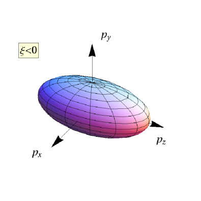
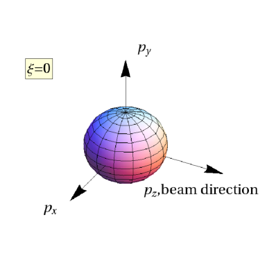
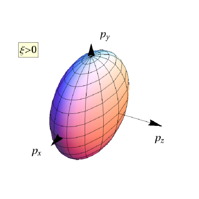
Figure 2.1: (Color online) Prolate (upper left part), isotropic (upper right part), and oblate (lower part) configurations of the distribution functions in momentum space.

2.5 Moments of the kinetic equations

For both the exact treatment of the kinetic equations (2.1) and construction of their approximation in the form of aHydro equations, it is necessary to consider moments of the kinetic equations in the momentum space. In this section, we clarify how such moments are defined. In the following section, we consider separately the zeroth and the first moments, as they are related to the baryon number and energy-momentum conservations.

In our approach, all particles are assumed to be on the mass shell, $p^{2}=p\cdot p=m^{2}$, hence we can use the momentum integration measure defined by Eq. (1.15). Gluons are always treated as massless particles, while quarks have a finite constant mass $m$.

We define the $n$-th moment operator (average) in the momentum space by the expression

$$\hat{{\cal I}}^{\mu_{1}\cdots\mu_{n}}(\dots)\equiv\int\!dP\,p^{\mu_{1}}p^{\mu_{2}}\cdots p^{\mu_{n}}(\dots),$$ (2.20)

with the zeroth moment operator defined by

$$\hat{{\cal I}}(\dots)\equiv\int\!dP\,(\dots).$$ (2.21)

Acting with $\hat{{\cal I}}^{\mu_{1}\cdots\mu_{n}}$ on the distribution functions $f_{\rm s}(x,p)$ and multiplying them by the degeneracy factors $k_{\rm s}$, one obtains the $n$-th moments of the distribution functions

$${\cal I}_{\rm s}^{\mu_{1}\cdots\mu_{n}} \equiv k_{\rm s}\,\hat{{\cal I}}^{\mu_{1}\cdots\mu_{n}}f_{\rm s}(x,p).$$ (2.22)

Here $k_{\rm s}\equiv g_{\rm s}/(2\pi)^{3}$, with $g_{{Q}}=g_{{Q^{\pm}}}=3\times 2\times N_{f}$ and $g_{G}=8\times 2$ being the internal degeneracy factors for (anti)quarks and gluons, respectively. In our calculations we assume that we deal with two (up and down) quark flavors with equal masses, which reflects the SU(2) isospin symmetry.

Using these definitions, the first, second, and third moments of the distribution functions read

$$N_{\rm s}^{\mu}(x) \equiv {\cal I}_{\rm s}^{\mu}=k_{\rm s}\int\!dP\,p^{\mu}f_{\rm s}(x,p),$$ (2.23)

$$T_{\rm s}^{\mu\nu}(x) \equiv {\cal I}_{\rm s}^{\mu\nu}=k_{\rm s}\int\!dP\,p^{\mu}p^{\nu}f_{\rm s}(x,p),$$ (2.24)

$$\Theta_{\rm s}^{\lambda\mu\nu}(x) \equiv {\cal I}_{\rm s}^{\lambda\mu\nu}=k_{\rm s}\int\!dP\,p^{\lambda}p^{\mu}p^{\nu}f_{\rm s}(x,p).$$ (2.25)

Equation (2.23) defines the particle number current, while Eq. (2.24) defines the energy-momentum tensor of the species “${\rm s}$”, respectively . In addition, we define the baryon number current

$$B^{\mu}(x) \equiv \sum_{\rm s}q_{\rm s}\,N_{\rm s}^{\mu}(x)=\frac{k_{{Q}}}{3}\int\!dP\,p^{\mu}\left[\vphantom{\frac{}{}}\!f_{Q^{+}}(x,p)-f_{Q^{-}}(x,p)\right],$$ (2.26)

where $q_{\rm s}=\left\{1/3,-1/3,0\right\}$ is the baryon number for quarks, antiquarks, and gluons, respectively. The total particle number current and total energy-momentum tensor read

$$N^{\mu}(x) = \sum_{\rm s}N_{\rm s}^{\mu}(x),$$ (2.27)

$$T^{\mu\nu}(x) = \sum_{\rm s}T_{\rm s}^{\mu\nu}(x).$$ (2.28)

We now consider the $n$-th moments of the kinetic equations (2.1), which are obtained by acting with the operator $\hat{{\cal I}}^{\mu_{1}\cdots\mu_{n}}$ given by (2.20) on their left- and right-hand sides and multiplying them by the degeneracy factors $k_{\rm s}$. The zeroth and first moments have the form

$$k_{\rm s}\,\hat{{\cal I}}p^{\mu}\partial_{\mu}f_{\rm s}(x,p) = k_{\rm s}\,\hat{{\cal I}}p^{\mu}U_{\mu}\frac{f_{{\rm s},{\rm eq}}(x,p)-f_{\rm s}(x,p)}{\tau_{\rm eq}},$$ (2.29)

$$k_{\rm s}\,\hat{{\cal I}}^{\nu}p^{\mu}\partial_{\mu}f_{\rm s}(x,p) = k_{\rm s}\,\hat{{\cal I}}^{\nu}p^{\mu}U_{\mu}\frac{f_{{\rm s},{\rm eq}}(x,p)-f_{\rm s}(x,p)}{\tau_{\rm eq}},\,\,\,\,\,\,$$ (2.30)

which, with the help of Eqs. (2.22)–(2.24), may be rewritten as

$$\partial_{\mu}{{N}}^{\mu}_{\rm s} = U_{\mu}\frac{{N}^{\mu}_{{\rm s},{\rm eq}}-{N}^{\mu}_{{\rm s}}}{\tau_{\rm eq}},$$ (2.31)

$$\partial_{\mu}{{T}}^{\mu\nu}_{\rm s} = U_{\mu}\frac{{T}^{\mu\nu}_{{\rm s},{\rm eq}}-{T}^{\mu\nu}_{{\rm s}}}{\tau_{\rm eq}}.$$ (2.32)

2.6 Landau matching conditions

Taking difference between ${\rm s}={Q^{+}}$ and ${\rm s}={Q^{-}}$ components of Eqs. (2.31) we obtain the baryon current evolution equation

$$\partial_{\mu}{{B}}^{\mu} = U_{\mu}\frac{{B}^{\mu}_{\rm eq}-{B}^{\mu}}{\tau_{\rm eq}}.$$ (2.33)

Similarly, by taking the sum over ${\rm s}$ components of Eqs. (2.32) and using Eq. (2.28) one gets the total energy and momentum conservation equation

$$\partial_{\mu}{{T}}^{\mu\nu} = U_{\mu}\frac{{T}^{\mu\nu}_{\rm eq}-{T}^{\mu\nu}}{\tau_{\rm eq}}.$$ (2.34)

In order to have the baryon number conserved it is required that the left-hand side of Eq. (2.33) vanishes, $\partial_{\mu}{{B}}^{\mu}=0$. The latter implies vanishing of the right-hand side of Eq. (2.33), which leads to the Landau matching condition for baryon current

$$U_{\mu}{B}^{\mu}_{\rm eq}=U_{\mu}{B}^{\mu}.$$ (2.35)

Analogously, the energy and momentum conservation means that the left-hand side of Eq. (2.34) vanishes, $\partial_{\mu}{{T}}^{\mu\nu}=0$. This condition results in vanishing of the right-hand side of Eq. (2.34), which leads to the Landau matching condition for energy and momentum

$$U_{\mu}{T}^{\mu\nu}_{\rm eq}=U_{\mu}{T}^{\mu\nu}.$$ (2.36)

Equations (2.35) and (2.36) have very natural physics interpretation. They tell us that the baryon number density ${\cal B}_{\rm eq}$ and the energy density ${\cal E}_{\rm eq}$ obtained with the reference equilibrium distribution functions $f_{{\rm s},{\rm eq}}(x,p)$ should be the same as ${\cal B}$ and ${\cal E}$ obtained with the actual nonequilibrium distributions $f_{{\rm s}}(x,p)$ . In a certain way, the Landau matching conditions define “the closest” equilibrium distributions to the actual ones — the former should render the same densities of the conserved currents as the latter. Using Eqs. (2.35) and (2.36), at any spacetime point $x$ we can determine effective temperature $T(x)$ and effective chemical potential $\mu(x)$, and use them to define the values of the equilibrium distribution functions. In this way, the kinetic equations (2.1) become a well-defined initial-value problem, which we aim to tackle in the following sections.

2.7 Tensor decomposition

We close this chapter with a section discussing algebraic structures of tensors used in our approach. Of special importance are the structures obtained for equilibrium and anisotropic RS distributions.

2.7.1 Basis vectors

For further use, it is convenient to treat the basis introduced in Sec. 2.2 in a more general way. To do so, we introduce the notation where $A$, $B$, $C$ $\in\left[U,X,Y,Z\right]$. In the local rest frame (LRF) we have

$$U^{\mu}_{\rm LRF}=(1,0,0,0),$$

$$X^{\mu}_{\rm LRF}=(0,1,0,0),$$

$$Y^{\mu}_{\rm LRF}=(0,0,1,0),$$

$$Z^{\mu}_{\rm LRF}=(0,0,0,1)\,.$$ (2.37)

Using Eqs. (2.7.1) one may express the metric tensor as [64]

$$g^{\mu\nu}=U^{\mu}U^{\nu}-\sum_{A\neq U}A^{\mu}A^{\nu}\,.$$ (2.38)

The projector on the space orthogonal to the four-velocity, $\Delta^{\mu\nu}\equiv g^{\mu\nu}-U^{\mu}U^{\nu}$, then takes the form

$$\Delta^{\mu\nu}=-\sum_{A\neq U}A^{\mu}A^{\nu}\,,$$ (2.39)

and satisfies the conditions $U_{\mu}\Delta^{\mu\nu}=0$, $\Delta^{\mu}_{\,\,\,\alpha}\Delta^{\alpha\nu}=\Delta^{\mu\nu}$ and $\Delta^{\mu}_{\,\,\,\mu}=3$. The basis (2.7.1) is a unit one in the sense that

$$A\cdot B=\begin{cases}\hphantom{-}0&\hbox{for }A\neq B,\\ \hphantom{-}1&\hbox{for }A=B=U,\\ -1&\hbox{for }A=B\neq U,\end{cases}$$ (2.40)

and complete so that any four-vector may be decomposed in the basis $\{A\}$. In particular, one may express the particle number flux as follows

$$N_{\rm s}^{\mu}(x) = \sum_{A}n_{A}^{{\rm s}}A^{\mu},$$ (2.41)

where the coefficients $n_{A}^{{\rm s}}$, due to Eqs. (2.40), are given by the projections

$$n_{A}^{{\rm s}} = A_{\mu}^{\,}N_{\rm s}^{\mu}(x)\,A^{2},$$ (2.42)

with $A^{2}=A\cdot A$ (note that $A^{2}=-1$ for space-like four-vectors of the basis (2.7.1)). The tensorial basis for the rank-two tensors is constructed using tensor products of the basis four-vectors $\{A\otimes B\}$. Thus the decomposition of the energy-momentum tensor takes the form

$$T_{\rm s}^{\mu\nu}(x) = \sum_{A,B}t_{AB}^{{\rm s}}A^{\mu}B^{\nu},$$ (2.43)

with the components of $T_{\rm s}^{\mu\nu}(x)$ defined as

$$t_{AB}^{{\rm s}} = A_{\mu}^{\,}B_{\nu}^{\,}T_{\rm s}^{\mu\nu}(x)\,A^{2}B^{2}.$$ (2.44)

Following similar methodology one can construct the tensorial basis for the rank-three tensors allowing to decompose $\Theta_{\rm s}^{\mu\nu\lambda}$ tensor as follows

$$\Theta_{\rm s}^{\mu\nu\lambda}(x) = \sum_{A,B,C}c_{ABC}^{{\rm s}}A^{\mu}B^{\nu}C^{\lambda},$$ (2.45)

where the coefficients $c_{ABC}^{{\rm s}}$ are defined through the expression

$$c_{ABC}^{{\rm s}} = A_{\mu}^{\,}B_{\nu}^{\,}C_{\lambda}^{\,}\Theta_{\rm s}^{\mu\nu\lambda}(x)\,A^{2}B^{2}C^{2}.$$ (2.46)

Using Eqs. (2.23)–(2.25) in Eqs. (2.42), (2.44) and (2.46) one gets

$$n_{A}^{{\rm s}} = k_{\rm s}\int\!dP\,\left(p\cdot A\right)A^{2}f_{\rm s}(x,p),$$ (2.47)

$$t_{AB}^{{\rm s}} = k_{\rm s}\int\!dP\,\left(p\cdot A\right)\left(p\cdot B\right)A^{2}B^{2}f_{\rm s}(x,p),$$ (2.48)

$$c_{ABC}^{{\rm s}} = k_{\rm s}\int\!dP\,\left(p\cdot A\right)\left(p\cdot B\right)\left(p\cdot C\right)A^{2}B^{2}C^{2}f_{\rm s}(x,p).$$ (2.49)

2.7.2 Equilibrium densities

In the case of equilibrium distribution functions $f_{{\rm s},{\rm eq}}(x,p)=f_{{\rm s},{\rm eq}}(p\cdot U(x))$, as defined by Eqs. (2.14) and (2.15), which, due to momentum isotropy, are invariant with respect to $SO(3)$ rotations in the three-momentum space, by the symmetry of the integrands in Eqs. (2.47)–(2.48) one has

$$n_{A}^{{\rm s},{\rm eq}} = k_{\rm s}\int\!dP\,\left(p\cdot A\right)A^{2}f_{{\rm s},{\rm eq}}=0\quad\hbox{if }A\neq U,$$ (2.50)

$$t_{AB}^{{\rm s},{\rm eq}} = k_{\rm s}\int\!dP\,\left(p\cdot A\right)\left(p\cdot B\right)A^{2}B^{2}f_{{\rm s},{\rm eq}}=0\quad\hbox{if }A\neq B.$$ (2.51)

Hence for the momentum-isotropic state Eqs. (2.41) and (2.43) have the following structure

$$N_{{\rm s},{\rm eq}}^{\mu}(x) = {\cal N}^{{\rm s},{\rm eq}}U^{\mu},$$ (2.52)

$$T_{{\rm s},{\rm eq}}^{\mu\nu}(x) = {\cal E}^{{\rm s},{\rm eq}}U^{\mu}U^{\nu}-{\cal P}^{{\rm s},{\rm eq}}\Delta^{\mu\nu},$$ (2.53)

with

$${\cal N}^{{\rm s},{\rm eq}}=n_{U}^{{\rm s},{\rm eq}},\quad{\cal E}^{{\rm s},{\rm eq}}=t_{UU}^{{\rm s},{\rm eq}},\quad{\cal P}^{{\rm s},{\rm eq}}=t_{XX}^{{\rm s},{\rm eq}}=t_{YY}^{{\rm s},{\rm eq}}=t_{ZZ}^{{\rm s},{\rm eq}},$$ (2.54)

being the particle density, energy density, and pressure in equilibrium, respectively. For a certain particle species ,,s”, Eqs. (2.52)–(2.53) define the energy-momentum tensor and the particle number flux of the perfect fluid, see Sec. 1.2.2. Explicit forms of these expressions are given in App. A.2 that uses results of App. A.1. Analogous calculation for the second moment (2.25), with the equilibrium distributions (2.14) and (2.15), gives

$$\Theta_{{\rm s},{\rm eq}}^{\mu\nu}(x) = \vartheta_{U}^{{\rm s},{\rm eq}}\,U^{\lambda}U^{\mu}U^{\nu}\,-\,\vartheta^{{\rm s},{\rm eq}}\,\left(U^{\lambda}\Delta^{\mu\nu}+U^{\mu}\Delta^{\lambda\nu}+U^{\nu}\Delta^{\lambda\mu}\right),$$ (2.55)

where $\vartheta_{U}^{{\rm s},{\rm eq}}=c_{UUU}^{{\rm s},{\rm eq}}$, and $\vartheta^{{\rm s},{\rm eq}}=c_{UXX}^{{\rm s},{\rm eq}}=c_{UYY}^{{\rm s},{\rm eq}}=c_{UZZ}^{{\rm s},{\rm eq}}$. The explicit expressions for variables $\vartheta$ are presented in App. B.

2.7.3 Anisotropic densities

The distributions defined by Eqs. (2.18) and (2.19) are invariant only with respect to $SO(2)$ rotations around the $z$ direction in the three-momentum space. In this case one still has

$$n_{A}^{{\rm s},{\rm a}} = 0\quad\hbox{if }A\neq U,$$ (2.56)

$$t_{AB}^{{\rm s},{\rm a}} = 0\quad\hbox{if }A\neq B,$$ (2.57)

however, in this case, Eqs. (2.23) and (2.24) have the following structure [120]

$$N_{{\rm s},{\rm a}}^{\mu}(x) = {\cal N}^{{\rm s},{\rm a}}U^{\mu},$$ (2.58)

$$T_{{\rm s},{\rm a}}^{\mu\nu}(x) = {\cal E}^{{\rm s},{\rm a}}U^{\mu}U^{\nu}-{\cal P}^{{\rm s},{\rm a}}_{T}\Delta_{T}^{\mu\nu}+{\cal P}^{{\rm s},{\rm a}}_{L}Z^{\mu}Z^{\nu},$$ (2.59)

with

$${\cal N}^{{\rm s},{\rm a}} = n_{U}^{{\rm s},{\rm a}},\quad{\cal E}^{{\rm s},{\rm a}}=t_{UU}^{{\rm s},{\rm a}},\quad{\cal P}^{{\rm s},{\rm a}}_{T}=t_{XX}^{{\rm s},{\rm a}}=t_{YY}^{{\rm s},{\rm a}},\quad{\cal P}^{{\rm s},{\rm a}}_{L}=t_{ZZ}^{{\rm s},{\rm a}}.$$ (2.60)

Here $\Delta_{T}^{\mu\nu}=-\left(X^{\mu}X^{\nu}+Y^{\mu}Y^{\nu}\right)$ is the projection operator on the direction orthogonal to $U$ and $Z$. Explicit forms of Eqs. (2.60) are given in App. A.1. For the anisotropic distributions (2.18) and (2.19) we also find that

$$\Theta_{{\rm s},{\rm a}}^{\lambda\mu\nu} = \vartheta_{U}^{{\rm s},{\rm a}}\,U^{\lambda}U^{\mu}U^{\nu}$$

$$- \,\vartheta_{T}^{{\rm s},{\rm a}}\,\left(U^{\lambda}\Delta^{\mu\nu}_{T}+U^{\mu}\Delta^{\lambda\nu}_{T}+U^{\nu}\Delta^{\lambda\mu}_{T}\right)$$

$$+ \,\vartheta_{L}^{{\rm s},{\rm a}}\,\left(U^{\lambda}Z^{\mu}Z^{\nu}+U^{\mu}Z^{\lambda}Z^{\nu}+U^{\nu}Z^{\lambda}Z^{\mu}\right),$$ (2.61)

where $\vartheta_{U}^{{\rm s},{\rm a}}=c_{UUU}^{{\rm s},{\rm a}}$, $\vartheta_{T}^{{\rm s},{\rm a}}=c_{UXX}^{{\rm s},{\rm a}}=c_{UYY}^{{\rm s},{\rm a}}$, and $\vartheta_{L}^{{\rm s},{\rm a}}=c_{UZZ}^{{\rm s},{\rm a}}$. For the explicit expressions for variables $\vartheta$ see App. B.

Chapter 3 Exact solutions of kinetic equations

In order to solve the Landau matching conditions (2.35) and (2.36) we need to know the form of the distribution functions $f_{{\rm s}}(x,p)$ that solve the kinetic equations (2.1). In general, such solutions are difficult to find, and (2.1) may be at best solved numerically. However, it is possible to find formal analytic solutions of Eqs. (2.1) in the case where the system is boost invariant and transversally homogeneous. Below, we discuss this case in more detail.

3.1 Białas-Czyż boost-invariant variables $w$ and $v$

In the case of the one-dimensional system exhibiting symmetries discussed above it is convenient to use the variables $w$ and $v$ which are defined as follows [107, 108]

$$w = tp_{L}-zE_{p}=-\,\tau\,p\cdot Z,$$ (3.1)

$$v = tE_{p}-zp_{L}=\tau\,p\cdot U.$$ (3.2)

We note that for $z=0$ the variable $w$ reduces to the longitudinal momentum multiplied by the time coordinate, whereas the $v$ variable is reduced to the energy multiplied by $t$.

Since particles are on the mass shell, the variables $w$ and $v$ are related by the formula

$$v(\tau,w,p_{T}) = \sqrt{w^{2}+\left(m^{2}+p_{T}^{\,2}\right)\tau^{2}}.$$ (3.3)

Equations (3.1) and (3.2) can be inverted to express the energy and longitudinal momentum of a particle in terms of $w$ and $v$, namely

$$E_{p}=\frac{vt+wz}{\tau^{2}},\quad p_{L}=\frac{wt+vz}{\tau^{2}}.$$ (3.4)

The Lorentz invariant momentum-integration measure can be then written as

$$dP=\frac{d^{3}p}{E_{p}}=\frac{dw\,d^{2}p_{T}}{v}.$$ (3.5)

For boost-invariant systems, all scalar functions of space and time, such as the effective temperature $T$ and quark chemical potential $\mu$ may depend only on $\tau$. In addition, one can check that the phase-space distribution functions, which are Lorentz scalars, may depend only on the variables $\tau$, $w$, and ${\boldsymbol{p}}_{T}$. We use these properties in the next section.

3.2 Formal solutions of the kinetic equations

With the help of the boost-invariant variables $w$, $v$ and ${\boldsymbol{p}}_{T}$ we can rewrite Eqs. (2.1) in a simple form [24, 25, 121, 122]

$$\frac{\partial f_{\rm s}\left(\tau,w,{\boldsymbol{p}}_{T}\right)}{\partial\tau} = \frac{f_{{\rm s},{\rm eq}}\left(\tau,w,p_{T}\right)-f_{\rm s}\left(\tau,w,{\boldsymbol{p}}_{T}\right)}{\tau_{\rm eq}},$$ (3.6)

where the boost-invariant versions of the equilibrium distribution functions are straightforward to find using (3.1) and (3.2), namely

$$f_{{Q^{\pm}},{\rm eq}}(\tau,w,p_{T}) = h^{+}_{\rm eq}\left(\frac{\sqrt{\left(\frac{w}{\tau}\right)^{2}+p_{T}^{2}+m^{2}}\mp\mu}{T}\,\right),$$ (3.7)

$$f_{{G},{\rm eq}}(\tau,w,p_{T}) = h^{-}_{\rm eq}\left(\frac{\sqrt{\left(\frac{w}{\tau}\right)^{2}+p_{T}^{2}}}{T}\,\right).$$ (3.8)

Below we assume that distribution functions $f_{\rm s}\left(\tau,w,{\boldsymbol{p}}_{T}\right)$ are even functions of $w$, and depend only on the magnitude of ${\boldsymbol{p}}_{T}$,

$$f_{\rm s}(\tau,w,p_{T})=f_{\rm s}(\tau,-w,p_{T}).$$ (3.9)

The formal solutions of Eqs. (3.6) have the following form [24, 25, 121, 122]

$$f_{\rm s}(\tau,w,p_{T}) = D(\tau,\tau_{0})f_{\rm s}^{0}(w,p_{T})+\int\limits_{\tau_{0}}^{\tau}\frac{d\tau^{\prime}}{\tau_{\rm eq}^{\prime}}\ D(\tau,\tau^{\prime})f_{{\rm s},{\rm eq}}(\tau^{\prime},w,p_{T}),$$ (3.10)

where $f_{\rm s}^{0}(w,p_{T})\equiv f_{\rm s}(\tau_{0},w,p_{T})$ is the initial distribution function — we have introduced here the notation $\tau_{\rm eq}^{\prime}=\tau_{\rm eq}(\tau^{\prime})$ for the general case where the equilibration time may depend on the proper time.

Perhaps at this stage, it is worth to clarify what we mean by the exact solutions of the kinetic equations. The exact solutions are high-accuracy numerical solutions of Eq. (3.10). They are usually obtained by the iterative method described in more detail below. Hence, the exact solutions are obtained with the help of combined analytic and numerical methods.

3.2.1 Damping function

In Eq. (3.10) we have introduced the damping function

$$D(\tau_{2},\tau_{1})=\mathrm{exp}\Bigg{[}-\int\limits_{\tau_{1}}^{\tau_{2}}\frac{d\tau^{\prime\prime}}{\tau_{\rm eq}(\tau^{\prime\prime})}\Bigg{]}.$$ (3.11)

The function $D(\tau_{2},\tau_{1})$ satisfies the two differential relations:

$$\frac{\partial D(\tau_{2},\tau_{1})}{\partial\tau_{2}}=-\frac{D(\tau_{2},\tau_{1})}{\tau_{\rm eq}(\tau_{2})},\quad\frac{\partial D(\tau_{2},\tau_{1})}{\partial\tau_{1}}=\frac{D(\tau_{2},\tau_{1})}{\tau_{\rm eq}(\tau_{1})},$$ (3.12)

and converges to unity if the two arguments are the same,

$$D(\tau,\tau)=1.$$ (3.13)

These properties imply the identity [105]

$$1=D(\tau,\tau_{0})+\int\limits_{\tau_{0}}^{\tau}\frac{d\tau^{\prime}}{\tau_{\rm eq}(\tau^{\prime})}D(\tau,\tau^{\prime}).$$ (3.14)

For a constant relaxation time used in this work Eq. (3.11) reduces to a simple exponential function

$$D(\tau_{2},\tau_{1})=\exp\left[-\frac{\tau_{2}-\tau_{1}}{\tau_{\rm eq}}\right].$$ (3.15)

3.2.2 Initial distributions

In what follows we assume that the initial distributions $f_{\rm s}^{0}(w,p_{T})$ are given by the anisotropic RS forms $f_{{\rm s},{\rm a}}^{0}(w,p_{T})$ which follow from Eqs. (2.18) and (2.19),

$$f_{{Q^{\pm}},{\rm a}}(\tau_{0},w,p_{T})=h^{+}_{\rm eq}\left(\frac{\sqrt{\left(1+\xi_{Q}^{0}\right)\left(\frac{w}{\tau_{0}}\right)^{2}+m^{2}+p_{T}^{2}}\mp\lambda^{0}}{\Lambda_{Q}^{0}}\right),$$ (3.16)

$$f_{{G},{\rm a}}(\tau_{0},w,p_{T})=h^{-}_{\rm eq}\left(\frac{\sqrt{\left(1+\xi_{G}^{0}\right)\left(\frac{w}{\tau_{0}}\right)^{2}+p_{T}^{2}}}{\Lambda_{G}^{0}}\,\right).$$

Here $\xi_{\rm s}^{0}\equiv\xi_{\rm s}(\tau_{0})$, $\Lambda_{\rm s}^{0}\equiv\Lambda_{\rm s}(\tau_{0})$, and $\lambda^{0}\equiv\lambda(\tau_{0})$ are initial parameters.

One may ask a question how much restrictive our assumption about the initial conditions is. By looking at the formal solution of the kinetic equation (3.10) and the form of the damping function (3.15) we conclude that the contribution from the initial condition is exponentially damped. Hence, the initial conditions seem to have little impact on the equilibration process, although they may affect the early hydrodynamization stage. In order to check such effects we perform calculations for various initial anisotropies. Below we shall consider three cases for quark and gluon initial distributions: oblate-oblate, prolate-oblate, and prolate-prolate (respectively for quarks and gluons); see Section  2.4.

3.2.3 Moments of the exact solution and their tensor structure

Knowledge about the forms of the exact distribution functions (3.10) allows us to calculate their moments using Eqs. (2.23)–(2.25) and their tensor decompositions using Eqs. (2.41)–(2.49). The symmetry of the momentum integrals of (3.10), in our case, is dictated by the $SO(2)$ symmetry in momentum space of the anisotropic RS forms of the initial distribution functions (3.16)–(3.2.2). As a result the exact energy-momentum tensor and particle number flux have the same tensor structure as the ones for the anisotropic RS distributions (2.58)–(2.59), namely

$$N_{{\rm s}}^{\mu}(x) = {\cal N}^{{\rm s}}U^{\mu},$$ (3.17)

$$T_{{\rm s}}^{\mu\nu}(x) = {\cal E}^{{\rm s}}U^{\mu}U^{\nu}-{\cal P}^{{\rm s}}_{T}\Delta_{T}^{\mu\nu}+{\cal P}^{{\rm s}}_{L}Z^{\mu}Z^{\nu},$$ (3.18)

where the thermodynamic quantities

$${\cal N}^{{\rm s}} = n_{U}^{{\rm s}},\quad{\cal E}^{{\rm s}}=t_{UU}^{{\rm s}},\quad{\cal P}^{{\rm s}}_{T}=t_{XX}^{{\rm s}}=t_{YY}^{{\rm s}},\quad{\cal P}^{{\rm s}}_{L}=t_{ZZ}^{{\rm s}},$$ (3.19)

are defined in the App. A.3.

3.3 Baryon number conservation

We turn now to a discussion of the conservation laws for baryon number, energy, and momentum. This is a crucial element of our approach. Using the expression for the baryon number current (2.26) and decompositions (2.52) and (3.17) one may rewrite Eq. (2.35) as

$${\cal B}^{\rm eq}={\cal B},$$ (3.20)

where we define the equilibrium and exact baryon number densities as

$${\cal B}^{\rm eq}=\frac{1}{3}\left({\cal N}^{{Q^{+}},{\rm eq}}-{\cal N}^{{Q^{-}},{\rm eq}}\right),\qquad{\cal B}=\frac{1}{3}\left({\cal N}^{{Q^{+}}}-{\cal N}^{Q^{-}}\right),$$ (3.21)

respectively. The explicit formula for ${\cal B}^{\rm eq}(\tau)$ is derived in App. A.2, see Eq. (A.33),

$${\cal B}^{\rm eq}(\tau)=\frac{16\pi k_{Q}T^{3}}{3}\sinh\left(\frac{\mu}{T}\right)\,{\cal H}_{\cal B}\left(\frac{m}{T},\frac{\mu}{T}\right),$$ (3.22)

where the function ${\cal H}_{\cal B}$ is defined by Eq. (A.21). The formula for ${\cal B}(\tau)$ is more complicated and is given in App. A.3, see Eq. (A.3). It contains an integral over the time history of the functions $T^{\prime}\equiv T(\tau^{\prime})$ and $\mu^{\prime}\equiv\mu(\tau^{\prime})$ in the range $\tau_{0}\leq\tau^{\prime}\leq\tau$. Consequently, Eq. (3.20) becomes an integral equation

$$T^{3}\sinh\left(\frac{\mu}{T}\right)\,{\cal H}_{\cal B}\left(\frac{m}{T},\frac{\mu}{T}\right) = \frac{\tau_{0}\left(\Lambda_{Q}^{0}\right)^{3}}{\tau\sqrt{1+\xi_{Q}^{0}}}\sinh\left(\frac{\lambda^{0}}{\Lambda_{Q}^{0}}\right)\,{\cal H}_{\cal B}\left(\frac{m}{\Lambda_{Q}^{0}},\frac{\lambda^{0}}{\Lambda_{Q}^{0}}\right)D(\tau,\tau_{0})$$ (3.23)

$$+\int\limits_{\tau_{0}}^{\tau}\frac{d\tau^{\prime}}{\tau_{\rm eq}^{\prime}}\ D(\tau,\tau^{\prime})\frac{\tau^{\prime}\left(T^{\prime}\right)^{3}}{\tau}\sinh\left(\frac{\mu^{\prime}}{T^{\prime}}\right)\,{\cal H}_{\cal B}\left(\frac{m}{T^{\prime}},\frac{\mu^{\prime}}{T^{\prime}}\right).$$

Equation (3.23) is a single equation for two functions, $T(\tau)$ and $\mu(\tau)$. The second necessary equation required for their determination is obtained from the Landau matching condition for the energy, which we discuss in the next section.

Meanwhile, it is interesting to notice that Eq. (3.23) can be rewritten as an integral equation for the function ${\cal B}(\tau)$, namely

$${\cal B}(\tau)=\frac{\tau_{0}}{\tau}{\cal B}(\tau_{0})D(\tau,\tau_{0})+\int\limits_{\tau_{0}}^{\tau}\frac{d\tau^{\prime}}{\tau_{\rm eq}^{\prime}}\frac{\tau^{\prime}}{\tau}{\cal B}(\tau^{\prime})\,D(\tau,\tau^{\prime}).$$ (3.24)

By differentiating (3.24) with respect to $\tau$ we get

$$\frac{d{\cal B}(\tau)}{d\tau}+\frac{{\cal B}(\tau)}{\tau}=0,$$ (3.25)

which is nothing else but the form of baryon number conservation law valid for the Bjorken geometry (in the original Bjorken paper [91] the same equation was obtained for the conserved entropy current). Equation (3.25) has a scaling solution

$${\cal B}(\tau)=\frac{\tau_{0}}{\tau}\,{\cal B}(\tau_{0}).$$ (3.26)

Combining (3.20) and (3.22) with (3.26) we find the equation

$$\sinh\left(\frac{\mu}{T}\right)\,{\cal H}_{\cal B}\left(\frac{m}{T},\frac{\mu}{T}\right)=\frac{3\tau_{0}{\cal B}(\tau_{0})}{16\pi k_{Q}\tau T^{3}},$$ (3.27)

which allows determining $\mu$ in terms of $T$ and $\tau$ for a given initial baryon number density. Unfortunately, in the general case we study (Fermi-Dirac statistics for quarks), Eq. (3.27) is an implicit equation for $\mu$. The situation simplifies in the case of classical statistics, where the function ${\cal H}_{\cal B}$ becomes independent of $\mu$. In this case, Eq. (3.27) can be used directly to determine $\mu$.

3.4 Energy-momentum conservation

Using the expression for the energy-momentum tensor (2.28) and decompositions (2.53) and (3.18) one may rewrite Eq. (2.36) as

$${\cal E}^{\rm eq}={\cal E},$$ (3.28)

where ${\cal E}^{\rm eq}$ and ${\cal E}$ contain contributions from quarks, antiquarks, and gluons

$${\cal E}^{\rm eq}={\cal E}^{{Q^{+}},{\rm eq}}+{\cal E}^{{Q^{-}},{\rm eq}}+{\cal E}^{G,{\rm eq}},$$ (3.29)

$${\cal E}={\cal E}^{{Q^{+}}}+{\cal E}^{Q^{-}}+{\cal E}^{G}.$$ (3.30)

Using Eqs. (A.26), (A.30), (A.3), and (LABEL:eq:eg) we obtain

$$T^{4}\left[\tilde{{\cal H}}^{+}\left(1,\frac{m}{T},-\frac{\mu}{T}\right)+\tilde{{\cal H}}^{+}\left(1,\frac{m}{T},+\frac{\mu}{T}\right)+r\tilde{{\cal H}}^{-}\left(1,0,0\right)\right]$$

$$=\left(\Lambda_{Q}^{0}\right)^{4}\left[\tilde{{\cal H}}^{+}\left(\frac{\tau_{0}}{\tau\sqrt{1+\xi_{Q}^{0}}},\frac{m}{\Lambda_{Q}^{0}},-\frac{\lambda^{0}}{\Lambda_{Q}^{0}}\right)+\tilde{{\cal H}}^{+}\left(\frac{\tau_{0}}{\tau\sqrt{1+\xi_{Q}^{0}}},\frac{m}{\Lambda_{Q}^{0}},+\frac{\lambda^{0}}{\Lambda_{Q}^{0}}\right)\right]D(\tau,\tau_{0})$$

$$+\int\limits_{\tau_{0}}^{\tau}\frac{d\tau^{\prime}}{\tau_{\rm eq}^{\prime}}\ D(\tau,\tau^{\prime})\left(T^{\prime}\right)^{4}\left[\tilde{{\cal H}}^{+}\left(\frac{\tau^{\prime}}{\tau},\frac{m}{T^{\prime}},-\frac{\mu^{\prime}}{T^{\prime}}\right)+\tilde{{\cal H}}^{+}\left(\frac{\tau^{\prime}}{\tau},\frac{m}{T^{\prime}},+\frac{\mu^{\prime}}{T^{\prime}}\right)\right]$$ (3.31)

$$+r\left[\left(\Lambda_{G}^{0}\right)^{4}\tilde{{\cal H}}^{-}\left(\frac{\tau_{0}}{\tau\sqrt{1+\xi_{Q}^{0}}},0,0\right)D(\tau,\tau_{0})+\int\limits_{\tau_{0}}^{\tau}\frac{d\tau^{\prime}}{\tau_{\rm eq}^{\prime}}\ D(\tau,\tau^{\prime})\left(T^{\prime}\right)^{4}\tilde{{\cal H}}^{-}\left(\frac{\tau^{\prime}}{\tau},0,0\right)\right],$$

where the functions $\tilde{{\cal H}}^{\pm}$ are defined by Eqs. (A.9) and $r$ is the ratio of the degeneracy factors

$$r=\frac{k_{G}}{k_{Q}}=\frac{g_{G}}{g_{Q}}=\frac{4}{3}.$$ (3.32)

Equations (3.23) and (3.31) are two integral equations that are sufficient to determine the proper-time dependence of the functions $T(\tau)$ and $\mu(\tau)$. This is done usually by the iterative method [109]. The two initial, to large extent arbitrary input functions $T_{\rm in}(\tau)$ and $\mu_{\rm in}(\tau)$ are used on the right-hand sides of (3.23) and (3.31) and the new values $T_{\rm out}(\tau)$ and $\mu_{\rm out}(\tau)$ are calculated from the left-hand sides. In the next iteration the new values are used as $T_{\rm in}(\tau)$ and $\mu_{\rm in}(\tau)$ on the right-hand sides to get updated values of $T_{\rm out}(\tau)$ and $\mu_{\rm out}(\tau)$. Such procedure is repeated until the updated values agree well with the initial values. We have found that the results converge with about 50 iterations if the final proper time is 5.0 fm. The time of the calculations grows quadratically with the final proper time.

Our use of the two coupled integral equations is similar to the case studied previously in [123]. We find that it is more straightforward than using (3.31) together with (3.27). However, the situation is different in the case of classical statistics, where (3.27) can be used to determine $\mu/T$ analytically. In this case, the expression for $\mu/T$ obtained from (3.27) may be substituted into (3.31) and we are left with a single integral equation for the function $T(\tau)$.

One may check, using (A.18) and (A.19), that Eq. (3.31) is consistent with the formula

$$\frac{d{\cal E}}{d\tau}=-\frac{{\cal E}+{\cal P}_{L}}{\tau},$$ (3.33)

where ${\cal P}_{L}={\cal P}_{L}^{{Q^{+}}}+{\cal P}_{L}^{Q^{-}}+{\cal P}_{L}^{G}$ is the total longitudinal pressure of the system. Equation (3.33) holds in general for the Bjorken expansion. It follows directly from the conservation law in the form $\partial_{\mu}T^{\mu\nu}=0$.

3.5 Basic observables

If the functions $T(\tau)$ and $\mu(\tau)$ are known, one can calculate all interesting observables using the formal expression for the solution of the kinetic equations. Above, we used the moments corresponding to baryon number and energy-momentum conservation. We have also introduced the longitudinal pressure ${\cal P}_{L}$ in Eq. (3.33). In a similar way one can calculate the transverse pressure ${\cal P}_{T}$. The difference between the longitudinal and transverse pressures shows how far our system is from local equilibrium. Analogous information can be obtained from the difference between the equilibrium, ${\cal P}_{\rm eq}$, and average, $(2{\cal P}_{T}+{\cal P}_{L})/3$, pressures. Analysis of such quantities will be presented in the following chapters in order to gain information about hydrodynamization and thermalization processes taking place in a non-equilibrium mixture.

Chapter 4 Numerical results with exact solutions

In this chapter, we present our main results obtained with exact solutions of the kinetic equations. In particular, we discuss here the hydrodynamization process and scaling properties of the ratio of longitudinal and transverse pressures.

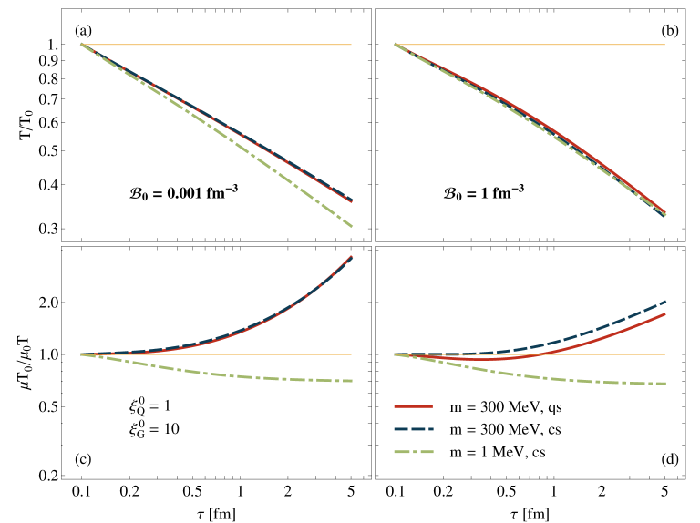
Figure 4.1: (Color online) Effective temperature $T$ (upper panels) and $\mu/T$ ratio (lower panels), shown as functions of the proper time $\tau$ and normalized to unity at the initial proper time $\tau=\tau_{0}$. Results correspond to the initial oblate-oblate configuration with the values of anisotropy parameters given in the figure. Three different types of lines correspond to three different choices of the statistics and the quark mass (the label “cs” denotes classical statistics used for both quarks and gluons, while the label “qs” denotes the use of Fermi-Dirac and Bose-Einstein statistics for quarks and gluons, respectively). Other parameters of the calculations are shown in the figure and discussed in the text.

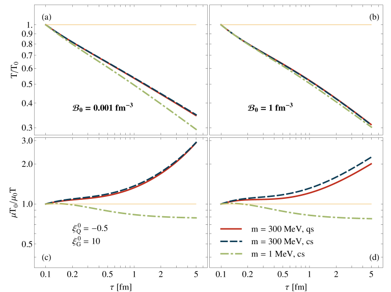
Figure 4.2: (Color online) Same as Fig. 4.1 but for the initial prolate-oblate configuration with the parameters given in the figure.

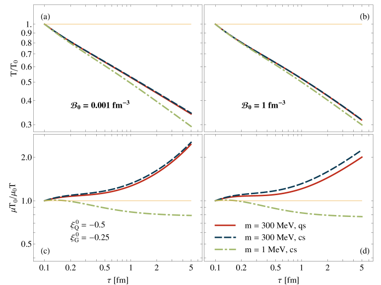
Figure 4.3: (Color online) Same as Figs. 4.1 and 4.2 but for the initial prolate-prolate configuration with the parameters given in the figure.

4.1 Initial conditions

In all the cases presented in this work, we use a constant equilibration time $\tau_{\rm eq}=0.25$ fm, which is the same for quark and gluon components.  The starting proper time is $\tau_{0}=0.1$ fm and the evolution continues till $\tau_{f}=5.0$ fm (or $\tau_{f}=10$ fm in several cases). The initial transverse momentum scales of quarks and gluons are taken identical: $\Lambda_{{Q}}^{0}=\Lambda_{{G}}^{0}=1$ GeV. The initial non-equilibrium chemical potential $\lambda_{0}$ is chosen in such a way that the initial baryon number density is either ${\cal B}_{0}~{}=$ 0.001 fm^-3 or ${\cal B}_{0}=$ 1 fm^-3, see Eq. (A.3).

Other initial conditions define different values of the anisotropy parameters. We use three sets of the values for $\xi_{{Q}}^{0}$ and $\xi_{{G}}^{0}$: i) $\xi_{{Q}}^{0}=1$ and $\xi_{{G}}^{0}=10$, ii) $\xi_{{Q}}^{0}=-0.5$ and $\xi_{{G}}^{0}=10$, and iii) $\xi_{{Q}}^{0}=-0.5$ and $\xi_{{G}}^{0}=-0.25$. They correspond to oblate-oblate, prolate-oblate, and prolate-prolate initial momentum distributions of quarks and gluons, respectively. Such initial values for $\xi_{{Q}}^{0}$ and $\xi_{{G}}^{0}$ were used previously in Ref. [95]. We note that different values of $\xi_{{Q}}^{0}$, $\xi_{{G}}^{0}$, and $\lambda_{0}$ imply different initial energy and baryon number densities, hence, due to matching conditions, also different initial values of $T_{0}$ and $\mu_{0}$. We also note that the oblate-oblate initial configuration is supported by the microscopic calculations which suggest that the initial transverse pressure is much higher than the longitudinal one [113, 114, 115, 116, 117, 118, 119].

We also perform our calculations for three different choices of the particle statistics and the quark mass: in the first case both quarks and gluons are described by the classical, Boltzmann statistics  and the quark mass is equal to 1 MeV , in the second case we use again the classical statistics but the quark mass is 300 MeV, finally, in the third case the quarks are described by the Fermi-Dirac statistics and have the mass of 300 MeV, while the gluons are described by the Bose-Einstein statistics. The gluon mass is always set equal to zero. The case with classical statistics, ${\cal B}_{0}=$ 0.001 fm^-3, and negligibly small quark mass of 1 MeV agrees well with the exact massless case studied in Ref. [95].This agreement is used as one of the checks of our present approach.

We note that the values of the initial conditions used in this work are to large extent arbitrary, as we want to analyze here only general features of the solutions of Eqs. (2.1) within a large span of the parameter space. With more specific systems in mind, one can freely amend the values of the initial parameters.

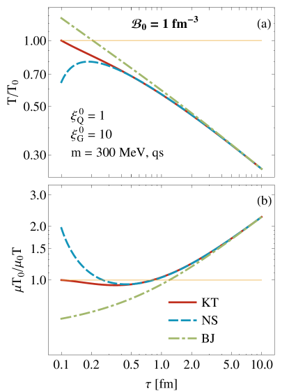
Figure 4.4: (Color online) Proper-time dependence of the ratios $T/T_{0}$ (a) and $\mu T_{0}/(\mu_{0}T)$ (b) obtained in the range $\tau_{0}<\tau<10$ fm from: kinetic theory (red solid lines), perfect-fluid hydrodynamics (green dot-dashed lines), and Navier-Stokes hydrodynamics (blue dashed lines). All results are normalized to the initial values $T_{0}$ and $\mu_{0}$ used in the kinetic theory. The initial values of temperature and chemical potential in the hydrodynamic calculations are chosen in such a way that the final values of $T$ and $\mu$ agree with the values found in the kinetic-theory calculation. The calculations are done for the oblate-oblate initial conditions with a finite quark mass of 300 MeV, quantum statistics, and ${\cal B}_{0}=$ 1 fm^-3.

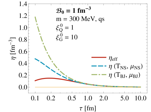
Figure 4.5: (Color online) Effective shear viscosity $\eta_{\rm eff}$ defined by Eq. (4.1) (red solid line) and the shear viscosity coefficients $\eta$ calculated using Eq. (4.2) for the two $T(\tau)$ and $\mu(\tau)$ profiles, found from the perfect-fluid hydrodynamics (green dot-dashed line) and from the Navier-Stokes equations (blue dashed line). The effective shear viscosity agrees well with the standard definition of $\eta$ for $\tau>0.5$ fm. The initial conditions are the same as in Fig. 4.4.

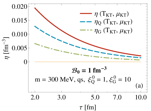
Figure 4.6: (Color online) Proper-time dependence of the shear viscosity of the mixture (red solid line), of the quark component (blue dashed line), and of the gluon component (green dot-dashed line), see Eqs. (4.2), (4.3) and (4.4), respectively, calculated within the kinetic theory. The initial conditions are the same as in Fig. 4.4.

4.2 Proper-time dependence of $T$ and $\mu/T$

Figures 4.1, 4.2 and 4.3 show the proper-time dependence of the effective temperature $T$ and $\mu/T$ ratio, which are normalized to unity at the initial time $\tau=\tau_{0}$. The two upper panels, (a) and (b), show temperature profiles, while the two lower panels, (c) and (d), show $\mu/T$. The two left panels, (a) and (c), correspond to the case ${\cal B}_{0}=$ 0.001 fm^-3, and the two right panels, (b) and (d), describe the case ${\cal B}_{0}=$ 1 fm^-3. The three figures correspond to three different initial conditions specified by the initial anisotropy parameters. Figures  4.1, 4.2, and 4.3 illustrate the effects of the finite mass and quantum statistics on the time evolution of $T$ and $\mu/T$.

We observe that the inclusion of the finite mass (for either classical or quantum statistics) has an important effect on the $\mu/T$ ratio. For $m=300$ MeV it asymptotically increases with time, while in the $m=1$ MeV case it approaches a constant, which is expected for the massless system in the Bjorken model assuming local equilibrium. The finite mass has a significant effect on the time dependence of the effective temperature. The latter decreases more slowly in the massive cases (especially in the ${\cal B}_{0}=$ 0.001 fm^-3 case). The effects of quantum statistics are most visible in the $\mu/T$ proper-time dependence.

To analyze the proper-time dependence of $T$ and $\mu/T$ in more detail, in Fig. 4.4 we compare the kinetic-theory (KT) results for the quantum, massive, and oblate-oblate case with hydrodynamic calculations. The latter are performed for the Bjorken perfect-fluid (BJ) and Navier-Stokes (NS) versions, see Appendix C for definitions of these frameworks. The initial values of temperature and chemical potential in the hydrodynamic calculations are chosen in such a way that the final values of $T$ and $\mu$ agree with the values found in the kinetic-theory calculation. Although such matching is required only for the last moment of the time evolution, we see that the hydrodynamic calculations approximate very well the kinetic-theory results within a few last fermis of the time evolution. As expected, we see that the Navier-Stokes approach reproduces better the exact kinetic-theory result, compared to the perfect-fluid calculation.

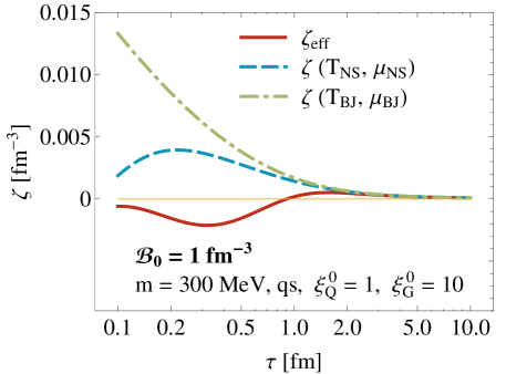
Figure 4.7: (Color online) Effective bulk viscosity $\zeta_{\rm eff}$ defined by Eq. (4.5) (red line) and the bulk viscosity coefficient $\zeta$ calculated with the help of Eq. (4.7) for the two $T(\tau)$ and $\mu(\tau)$ profiles, found from the perfect-fluid hydrodynamics (green dot-dashed line) and from the Navier-Stokes equations (blue dashed line). We find that the effective bulk viscosity agrees with the standard definition of $\zeta$ for $\tau>2$ fm. The initial conditions are the same as in Fig. 4.4.

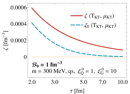
Figure 4.8: (Color online) Bulk viscosity coefficient $\zeta$ calculated with the help of Eq. (4.7) with the thermodynamic coefficients $\kappa_{1}$ and $\kappa_{2}$ determined for the whole quark-gluon system (red solid line) and the coefficient $\zeta_{0}$ obtained from Eq. (4.7) with $\kappa_{1}$ and $\kappa_{2}$ determined only for the quark component (blue dashed line). The initial conditions are the same as in Fig. 4.4.

4.3 Hydrodynamization

4.3.1 Shear sector

The results shown in Fig. 4.4 suggest that the non-equilibrium dynamics of the system enters rather fast the hydrodynamic regime described by the NS equations (at the stage where deviations from local equilibrium are still substantial). Such a phenomenon was identified first in the context of AdS/CFT calculations [116] and is known now as the hydrodynamization process. To illustrate this behavior in our case, we show in Fig. 4.5 the proper-time dependence of the effective shear viscosity coefficient $\eta_{\rm eff}$ defined by the expression [25] 

$$\eta_{\rm eff}=\frac{\tau}{2}\left({\cal P}_{T}-{\cal P}_{L}\right),$$ (4.1)

see Eqs. C.3. The effective shear viscosity (solid red line in Fig. 4.5) is compared with the standard shear viscosity coefficient, $\eta$, valid for the system close to equilibrium. For the quark-gluon mixture the latter is defined as the sum of the quark and gluon coefficients, 

$$\eta=\eta_{Q}+\eta_{G},$$ (4.2)

where following [125], see also [126, 127, 128], we use

$$\eta_{Q}=\frac{g_{Q}\tau_{\rm eq}}{15T}\int\limits_{0}^{\infty}\frac{dp\,p^{6}}{2\pi^{2}(m^{2}+p^{2})}\left[f_{{Q^{+}},{\rm eq}}\left(1-f_{{Q^{+}},{\rm eq}}\right)+f_{{Q^{-}},{\rm eq}}\left(1-f_{{Q^{-}},{\rm eq}}\right)\right],$$ (4.3)

$$\eta_{G}=\frac{g_{G}\tau_{\rm eq}}{15T}\int\limits_{0}^{\infty}\frac{dp\,p^{4}}{2\pi^{2}}f_{{G},{\rm eq}}\left(1+f_{{G},{\rm eq}}\right).$$ (4.4)

The coefficient $\eta$ is calculated as a function of $T$ and $\mu$ obtained either from the perfect-fluid (green dot-dashed line in Fig. 4.5) or NS hydrodynamic calculation (blue dashed line in Fig. 4.5). In the two cases, we find that $\eta_{\rm eff}$ agrees very well with $\eta$ for $\tau>0.5$ fm which is about two times the relaxation time. Thus, in the shear sector, we observe a very fast approach to the hydrodynamic NS regime. It is important to notice that the agreement with the NS description is reached when $\eta$ is significantly different from zero, which supports the idea that the hydrodynamic description becomes appropriate before the system thermalizes, i.e., before the state of local thermal equilibrium with ${\cal P}_{T}\approx{\cal P}_{L}$ is reached.

In Fig. 4.6 we show the proper-time dependence of the shear viscosity of the mixture (red solid line) using the kinetic theory results and compare it with the shear viscosity of the quark component (blue dashed line) and the gluon component (green dot-dashed line), see Eqs. (4.2), (4.3) and (4.4), respectively. The initial conditions are the same as in Fig. 4.4. The results shown in Fig. 4.6 show that the shear viscosity of the mixture is dominated by the shear viscosity of quarks.

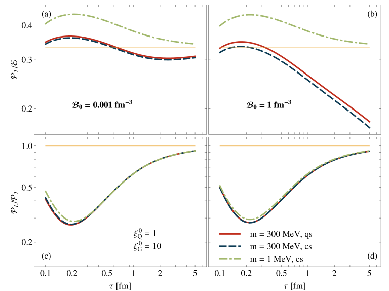
Figure 4.9: (Color online) ${\cal P}_{T}/{\cal E}$ (upper panels) and ${\cal P}_{L}/{\cal P}_{T}$ (lower panels) for the initially oblate-oblate system. Green dot-dashed lines correspond to “massless” quarks and classical distribution functions, navy blue dashed lines correspond to the massive quarks and classical distribution functions, while red solid lines are for massive quarks and quantum distributions. Left (right) panels describe the results for ${\cal B}_{0}=$ 0.001 fm^-3 (${\cal B}_{0}=$ 1 fm^-3).

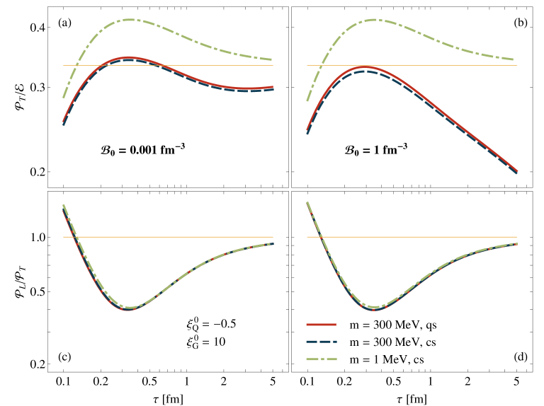
Figure 4.10: (Color online) Same as Fig. 4.9 but for the initially prolate-oblate system.

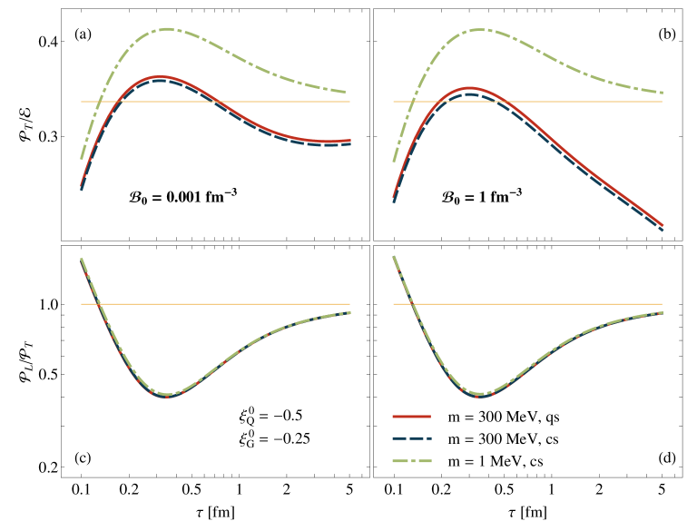
Figure 4.11: (Color online) Same as Fig. 4.9 but for the initially prolate-prolate system.

4.3.2 Bulk sector

Similarly to the shear-viscosity effects, we can analyze the bulk sector, where we define the effective bulk viscosity by the expression

$$\zeta_{\rm eff}=-\tau\Pi,$$ (4.5)

where $\Pi$ is the exact bulk pressure

$$\Pi=\frac{1}{3}\left({\cal P}_{L}+2{\cal P}_{T}-3{\cal P}^{\rm eq}\right).$$ (4.6)

In Fig. 4.7 the time dependence of the effective bulk viscosity is compared with the time dependence of the bulk viscosity coefficient given by the expression

$$\zeta = \frac{g_{Q}m^{2}\tau_{\rm eq}}{3T}\int\limits_{0}^{\infty}\frac{dp\,p^{2}}{2\pi^{2}}\left[\left(f_{{Q^{+}},{\rm eq}}\left(1-f_{{Q^{+}},{\rm eq}}\right)+f_{{Q^{-}},{\rm eq}}\left(1-f_{{Q^{-}},{\rm eq}}\right)\right)\left(\kappa_{1}-\frac{p^{2}}{3(m^{2}+p^{2})}\right)\right.$$ (4.7)

$$\hskip 99.58464pt\left.+\left(f_{{Q^{+}},{\rm eq}}\left(1-f_{{Q^{+}},{\rm eq}}\right)-f_{{Q^{-}},{\rm eq}}\left(1-f_{{Q^{-}},{\rm eq}}\right)\right)\frac{\kappa_{2}}{\sqrt{m^{2}+p^{2}}}\right],$$

where $\kappa_{1}$ and $\kappa_{2}$ are defined by the thermodynamic derivatives

$$\kappa_{1}(T,\mu)=\left(\frac{\partial{\cal P}^{{\rm eq}}}{\partial{\cal E}^{{\rm eq}}}\right)_{{\cal B}^{{\rm eq}}},\qquad\kappa_{2}(T,\mu)=\frac{1}{3}\left(\frac{\partial{\cal P}^{{\rm eq}}}{\partial{\cal B}^{{\rm eq}}}\right)_{{\cal E}^{{\rm eq}}}.$$ (4.8)

For a simple fluid with zero baryon density, the coefficient $\kappa_{1}$ becomes equal to the sound velocity squared. The steps leading to Eq. (4.7) are described in more detail in Appendix D. The form of (4.7) agrees with that given in [125] for fermions. There is, however, one important difference between our approach and that of [125]. In Ref. [125] a simple system of fermions is considered and (4.7) includes the derivatives (4.8) where only fermionic thermodynamic functions appear. In our case, we deal with a mixture and we have checked that (4.8) should include the total thermodynamic functions being the sums of quark and gluon contributions. Thus, although the bulk viscosity of a quark-gluon mixture is given by the formula known for massive quarks (and $\zeta=0$ if $m=0$), the use of the full thermodynamic functions in Eqs. (4.8) means that although gluons are considered massless they contribute to the bulk viscosity of the full system.

Similarly, as in the shear sector, we can see in Fig. 4.7 that $\zeta_{\rm eff}(\tau)$ approaches $\zeta(\tau)$, however, the agreement is reached for significantly larger times, $\tau>2$ fm. This means that the hydrodynamization of the bulk sector is slower and takes place after the hydrodynamization of the shear sector. Observations that the hydrodynamization in the shear sector may happen before the hydrodynamization in the bulk sector have been done recently in Ref. [129] within the gauge/gravity correspondence with the breaking of conformality, where the hydrodynamization in the bulk sector has been dubbed the EoSization process [130]. In this scenario first ${\cal P}_{L}$ and ${\cal P}_{T}$ tend to a common value ${\bar{\cal P}}\neq{\cal P}^{\rm eq}$ and, subsequently, ${\bar{\cal P}}$ approaches ${\cal P}^{\rm eq}$, which signals establishing equation of state (EOS) of the system.

To visualize the importance of the gluon degrees of freedom in expressions (4.8) for the bulk viscosity of the mixture in Fig. 4.8 we show the bulk viscosity coefficient $\zeta$ and compare it with the coefficient $\zeta_{0}$ that has been calculated in the same way as $\zeta$ except that the thermodynamic coefficients $\kappa_{1}$ and $\kappa_{2}$ of the former were calculated only for the quark component. We find that neglecting the gluon contribution in $\kappa_{1}$ and $\kappa_{2}$ changes substantially the values of $\zeta$ making it significantly smaller. This finding indicates that gluons, although, massless, contribute to the bulk viscosity of a quark-gluon mixture. The necessary requirement for this effect is, however, that quarks are massive.

4.3.3 ${\cal P}_{T}/{\cal E}$ and ${\cal P}_{L}/{\cal P}_{T}$

Figures 4.9, 4.10, and 4.11 correspond to Figs. 4.1, 4.2, and 4.3, respectively, and show the time dependence of the ratios ${\cal P}_{T}/{\cal E}$ (upper panels) and ${\cal P}_{L}/{\cal P}_{T}$ (lower panels). In the case of quarks with a very small mass (green dot-dashed lines) the ratios ${\cal P}_{T}/{\cal E}$ tend to 1/3 as expected for massless systems approaching local equilibrium. The ratios ${\cal P}_{L}/{\cal P}_{T}$ in all studied cases tend to unity which again reflects equilibration of the system. Interestingly, the ratios ${\cal P}_{L}/{\cal P}_{T}$ very weakly depend on the quark mass and the choice of the statistics.

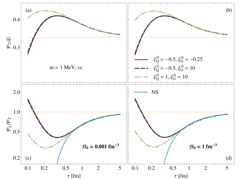
Figure 4.12: (Color online) ${\cal P}_{T}/{\cal E}$ (upper panels) and ${\cal P}_{L}/{\cal P}_{T}$ (lower panels) for “massless” quarks and classical distribution functions. Green dot-dashed, navy blue dashed, and red solid lines describe the results for the oblate-oblate, prolate-oblate, and prolate-prolate initial conditions. The blue dotted line describes $({\cal P}_{L}/{\cal P}_{T})_{\rm NS}$ obtained from the Navier-Stokes hydrodynamics. Left (right) panels describe the results for ${\cal B}_{0}=$ 0.001 fm^-3 (${\cal B}_{0}=$ 1 fm^-3).

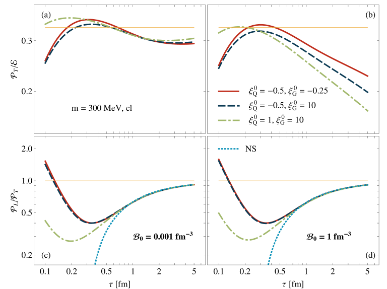
Figure 4.13: (Color online) Same as Fig. 4.12 but for massive quarks and classical statistics.

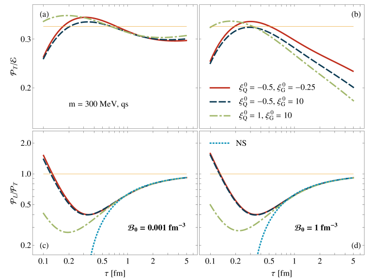
Figure 4.14: (Color online) Same as Fig. 4.12 but for massive quarks and quantum statistics.

4.4 Scaling properties

Each panel of Figs. 4.9, 4.10, and 4.11 shows our results obtained for different values of the quark mass and particle statistics but for the same initial anisotropies. In Figs. 4.12, 4.13, and 4.14 we rearrange this information showing in each panel our results obtained for different initial anisotropies, i.e., for oblate-oblate, prolate-oblate, and prolate-prolate initial quark and gluon distributions. Figures 4.12, 4.13, and 4.14 collect the results for different mass and statistics. The most striking feature of our results presented in these figures is that the ${\cal P}_{L}/{\cal P}_{T}$ ratios (shown in lower panels) converge to the same values, although they describe the system evolutions starting from completely different initial conditions.

The origin of this behavior can be found if we analyze the NS formula for the ${\cal P}_{L}/{\cal P}_{T}$ ratio. Let us first consider the massless case where we may neglect the bulk viscosity and write

$$\left(\frac{{\cal P}_{L}}{{\cal P}_{T}}\right)_{\rm NS}=\frac{{\cal P}^{{Q},\rm eq}-4\eta_{Q}/(3\tau)+{\cal P}^{{G},\rm eq}-4\eta_{G}/(3\tau)}{{\cal P}^{{Q},\rm eq}+2\eta_{Q}/(3\tau)+{\cal P}^{{G},\rm eq}+2\eta_{G}/(3\tau)}.$$ (4.9)

Assuming in addition that the baryon number density is zero, we may use the following relations connecting the shear viscosity with equilibrium pressure :

$$\eta_{Q}=\frac{4}{5}\tau_{\rm eq}{\cal P}^{{Q},\rm eq},\quad\eta_{G}=\frac{4}{5}\tau_{\rm eq}{\cal P}^{{G},\rm eq}.$$ (4.10)

It is interesting to note that the coefficient 4/5 is the same for quarks and gluons, hence

$$\left(\frac{{\cal P}_{L}}{{\cal P}_{T}}\right)_{\rm NS}=\frac{1-16\tau_{\rm eq}/(15\tau)}{1+8\tau_{\rm eq}/(15\tau)},$$ (4.11)

which explains the late-time dependence of ${\cal P}_{L}/{\cal P}_{T}$ on the proper time only, observed in panel (c) of Fig. 4.12. We note that if the relaxation time is inversely proportional to the temperature, Eq. (4.11) indicates that $\left({\cal P}_{L}/{\cal P}_{T}\right)_{\rm NS}$ depends on the product of $\tau$ and $T$, which is expected for conformal systems and related to the existence of a hydrodynamic attractor for such systems [59, 98, 99, 100, 101, 102]. It turns out that the inclusion of the finite mass and baryon chemical potential (with the values studied in this work) affects very little Eqs. (4.10) connecting the shear viscosity with pressure. The main difference is that the coefficient 4/5 is slightly changed. It should be replaced by an effective value obtained for the studied range of $T$ and $\mu$.

To analyze the $\left({\cal P}_{L}/{\cal P}_{T}\right)_{\rm NS}$ ratio in a general case in Fig. 4.15 we plot it as a function of two variables, $\tau_{\rm eq}/\tau$ and $m/T$, for a fixed value of $\mu$. The left panel of Fig. 4.15 shows the contour plot of $\left({\cal P}_{L}/{\cal P}_{T}\right)_{\rm NS}$ in the case where quantum statistics are used and $\mu=0$. The fact that the contour (red dashed) lines have horizontal shapes indicates that $\left({\cal P}_{L}/{\cal P}_{T}\right)_{\rm NS}$ depends effectively only on $\tau_{\rm eq}/\tau$ ratio (except for the region where $\tau\approx\tau_{\rm eq}$ and $T\approx m/5$). The red dashed lines overlap with solid black lines corresponding to the result for the case of classical statistics. It shows that quantum statistics have a negligible effect on $\left({\cal P}_{L}/{\cal P}_{T}\right)_{\rm NS}$ in the studied, rather broad range of $\tau_{\rm eq}/\tau$ and $m/T$. These observations explain similarities of the close-to-equilibrium behavior of $\left({\cal P}_{L}/{\cal P}_{T}\right)_{\rm NS}$ in the left panels of Figs. 4.9, 4.10, and 4.11. The right panel of Fig. 4.15 shows the contour plot of $\left({\cal P}_{L}/{\cal P}_{T}\right)_{\rm NS}$ for $\mu/T=2$. In this case, we find again a weak dependence on $m/T$ as compared to the case of classical statistics and $\mu=0$ represented by the solid black lines. Again this helps to understand the similarities of the right and left panels of Figs. 4.9, 4.10, and 4.11.

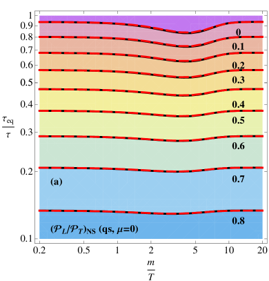
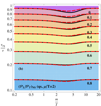
Figure 4.15: (Color online) Contour plots of $({\cal P}_{L}/{\cal P}_{T})_{\rm NS}$ obtained for the Navier-Stokes hydrodynamics for $\mu=0$ (a) and $\mu/T=2$ (b). In the two cases quarks and gluons are described by quantum statistics. The solid black lines together with the contour shading represent the classical baryon-free system.

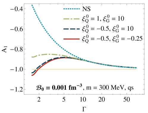
Figure 4.16: (Color online) The quantity $A_{1}$ plotted as a function of $\Gamma$ for three different initial anisotropies, finite quark mass, and quantum statistics.

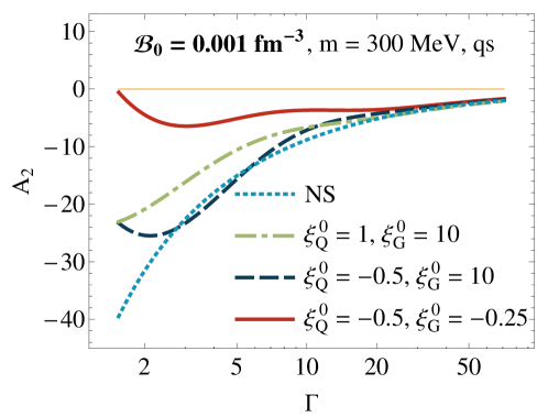
Figure 4.17: (Color online) Same as Fig. 4.16 but for $A_{2}$ vs. $\Gamma$.

4.4.1 Remarks on non-conformal attractors

In a very recent paper [131] it has been suggested by Romatschke to look for attractor behavior by studying the quantities

$$A_{1}=\frac{\tau d{\cal E}}{({\cal E}+{\cal P}_{\rm eq})d\tau}$$ (4.12)

and

$$A_{2}=\frac{2{\cal P}_{T}+{\cal P}_{L}-3{\cal P}_{\rm eq}}{\zeta T}$$ (4.13)

as functions of the variable

$$\Gamma=\tau\left[\frac{4}{3}\frac{\eta}{{\cal E}+{\cal P}_{\rm eq}}+\frac{\zeta}{{\cal E}+{\cal P}_{\rm eq}}\right]^{-1}.$$ (4.14)

Note that in Eqs. (4.12)–(4.14) we used boost invariance to simplify our notation.

In Fig. 4.16 we show the function $A_{1}(\Gamma)$ obtained for three different initial anisotropies studied in this work. To get the connection with [131] we consider the case with negligible baryon number density. Otherwise, we include the finite mass of quarks and quantum statistics. Figure  4.16 shows that first the lines corresponding to three different initial conditions converge and later approach the Navier-Stokes line. This observation supports the existence of a non-conformal attractor for $A_{1}$ in our system.

Figure 4.17 shows similar results as Fig. 4.16 but for $A_{2}(\Gamma)$. In this case, the lines corresponding to different initial conditions converge with each other only in the NS regime. Hence, our present results are insufficient to demonstrate the existence of an attractor for $A_{2}$. Further study of this behavior is planned for our future investigations.

Chapter 5 Anisotropic hydrodynamics for a mixture

5.1 Anisotropic-hydrodynamics concept

In this Thesis, following the main ideas of anisotropic hydrodynamics (aHydro) [26, 27], we make an assumption that the exact solutions, $f_{{\rm s}}(x,p)$, of the kinetic equations (2.1) are very well approximated by the RS anisotropic distributions [84].

The use of the RS ansatz for the quark and gluon distributions means that we deal with seven unknown functions: $\xi_{Q},\Lambda_{Q},\xi_{G},\Lambda_{G},\lambda,\mu$, and $T$. Their time dependence will be determined by using a properly selected set of moments of Eqs. (2.1). In this work we follow Ref. [95] and use two equations constructed from the zeroth moments, one from the first moment, and two from the second moments. In addition, we use the Landau matching conditions that guarantee the baryon number and energy-momentum conservation .

5.2 Zeroth moments

The zeroth moments of the kinetic equations (2.1) give three scalar equations

$$\partial_{\mu}\left({\cal N}_{{Q^{\pm}},\rm a}U^{\mu}\right) = \frac{{\cal N}_{{Q^{\pm}},\rm eq}-{\cal N}_{{Q^{\pm}},\rm a}}{\tau_{\rm eq}},$$ (5.1)

$$\partial_{\mu}\left({\cal N}_{{G},\rm a}U^{\mu}\right) = \frac{{\cal N}_{{G},\rm eq}-{\cal N}_{{G},\rm a}}{\tau_{\rm eq}}.$$ (5.2)

To construct the hydrodynamic framework, we cannot use all the equations listed in (5.1) and (5.2), since this would lead to the overdetermined system . Therefore, following Ref. [95], we use only two equations constructed as linear combinations of (5.1) and (5.2). The first equation is obtained from the difference of the quark (${Q^{+}}$) and antiquark (${Q^{-}}$) components in Eqs. (5.1),

$$\frac{d}{d\tau}\left({\cal N}_{{Q^{+}},\rm a}-{\cal N}_{{Q^{-}},\rm a}\right)+\frac{{\cal N}_{{Q^{+}},\rm a}-{\cal N}_{{Q^{-}},\rm a}}{\tau} = \frac{{\cal N}_{{Q^{+}},\rm eq}-{\cal N}_{{Q^{-}},\rm eq}-\left({\cal N}_{{Q^{+}},\rm a}-{\cal N}_{{Q^{-}},\rm a}\right)}{\tau_{\rm eq}},$$ (5.3)

while the second equation is a linear combination of Eqs. (5.1) and (5.2),

$$\alpha\left(\frac{d{\cal N}_{Q,\rm a}}{d\tau}+\frac{{\cal N}_{{Q},\rm a}}{\tau}\right)+(1-\alpha)\left(\frac{d{\cal N}_{G,\rm a}}{d\tau}+\frac{{\cal N}_{{G},\rm a}}{\tau}\right)$$

$$=\alpha\,\frac{{\cal N}_{{Q},\rm eq}-{\cal N}_{{Q},\rm a}}{\tau_{\rm eq}}+(1-\alpha)\,\frac{{\cal N}_{{G},\rm eq}-{\cal N}_{{G},\rm a}}{\tau_{\rm eq}},$$ (5.4)

where the parameter $\alpha$ is a constant taken from the range $0\leq\alpha\leq 1$. To denote the sums of the contributions from quarks and antiquarks we use the symbol ${Q}$, for example

$$N_{Q}^{\mu}=N_{Q^{-}}^{\mu}+N_{Q^{+}}^{\mu},\quad{\cal N}_{{Q}}={\cal N}_{{Q^{-}}}+{\cal N}_{{Q^{+}}}.$$ (5.5)

By doing comparisons between the predictions of the kinetic theory and the results obtained with aHydro one can check which value of $\alpha$ is optimal. In Ref. [95] we found that the best cases corresponded to either $\alpha=0$ or $\alpha=1$. One may understand this behavior, since such values of $\alpha$ do not introduce any direct coupling between the quark and gluon sectors except for that included by the energy-momentum conservation, which is accounted for by the first moment — such a situation takes place in the case where kinetic equations are treated exactly. Our present investigations of more complex systems also favor the values $\alpha=0$ and $\alpha=1$. We return to this discussion in Chapter 6.

5.2.1 Baryon number conservation

Equation (5.3) leads directly to the constraint on the baryon number density

$$\frac{d{\cal B}_{\rm a}(\tau)}{d\tau}+\frac{{\cal B}_{\rm a}(\tau)}{\tau}=\frac{{\cal B}_{\rm eq}-{\cal B}_{\rm a}}{\tau_{\rm eq}}.$$ (5.6)

The conservation of the baryon number requires that both the left- and the right-hand sides of (5.6) vanish. This leads to two equations

$${\cal B}_{\rm a}(\tau)=\frac{{\cal B}_{\rm 0}\tau_{0}}{\tau}$$ (5.7)

and

$${\cal B}_{\rm a}(\tau)={\cal B}_{\rm eq}(\tau),$$ (5.8)

which lead to

$$\frac{\Lambda_{Q}^{3}}{\sqrt{1+\xi_{Q}}}\sinh\left(\frac{\lambda}{\Lambda_{Q}}\right)\,{\cal H}_{\cal B}\left(\frac{m}{\Lambda_{Q}},\frac{\lambda}{\Lambda_{Q}}\right)=T^{3}\sinh\left(\frac{\mu}{T}\right)\,{\cal H}_{\cal B}\left(\frac{m}{T},\frac{\mu}{T}\right)$$ (5.9)

and

$$\frac{16\pi k_{Q}T^{3}}{3}\sinh\left(\frac{\mu}{T}\right)\,{\cal H}_{\cal B}\left(\frac{m}{T},\frac{\mu}{T}\right)=\frac{{\cal B}_{\rm 0}\tau_{0}}{\tau}.$$ (5.10)

The function ${\cal H}_{\cal B}$ is defined explicitly in App. A.1.

The last two equations can be used to determine $\lambda$ and $\mu$ in terms of ${\cal B}_{\rm 0}\tau_{0}/\tau$, $T$, $\Lambda_{Q}$, and $\xi_{Q}$. Thus, in the following equations we may treat $\lambda$ and $\mu$ as known functions of other hydrodynamic variables. 

5.2.2 Sum of the zeroth moments

Equation (5.4) can be written in the form

$$\frac{d}{d\tau}\left[\alpha\Lambda_{Q}^{3}\left(\tilde{{\cal H}}_{\cal N}^{+}\left(\frac{1}{\sqrt{1+\xi_{Q}}},\frac{m}{\Lambda_{Q}},-\frac{\lambda}{\Lambda_{Q}}\right)+\tilde{{\cal H}}_{\cal N}^{+}\left(\frac{1}{\sqrt{1+\xi_{Q}}},\frac{m}{\Lambda_{Q}},+\frac{\lambda}{\Lambda_{Q}}\right)\right)\right.$$ (5.11)

$$\hskip 85.35826pt\left.+\,(1-\alpha)\,r\,\Lambda_{G}^{3}\tilde{{\cal H}}_{\cal N}^{-}\left(\frac{1}{\sqrt{1+\xi_{G}}},0,0\right)\right]$$

$$+\left(\frac{1}{\tau}+\frac{1}{\tau_{\rm eq}}\right)\left[\alpha\Lambda_{Q}^{3}\left(\tilde{{\cal H}}_{\cal N}^{+}\left(\frac{1}{\sqrt{1+\xi_{Q}}},\frac{m}{\Lambda_{Q}},-\frac{\lambda}{\Lambda_{Q}}\right)+\tilde{{\cal H}}_{\cal N}^{+}\left(\frac{1}{\sqrt{1+\xi_{Q}}},\frac{m}{\Lambda_{Q}},+\frac{\lambda}{\Lambda_{Q}}\right)\right)\right.$$

$$\hskip 85.35826pt\left.+\,(1-\alpha)\,r\,\Lambda_{G}^{3}\tilde{{\cal H}}_{\cal N}^{-}\left(\frac{1}{\sqrt{1+\xi_{G}}},0,0\right)\right]$$

$$= \frac{T^{3}}{\tau_{\rm eq}}\left[\alpha\left(\tilde{{\cal H}}_{\cal N}^{+}\left(1,\frac{m}{T},-\frac{\mu}{T}\right)+\tilde{{\cal H}}_{\cal N}^{+}\left(1,\frac{m}{T},+\frac{\mu}{T}\right)\right)+\,(1-\alpha)\,r\,\tilde{{\cal H}}_{\cal N}^{-}\left(1,0,0\right)\right].$$

Here we have introduced again the ratio of the internal degeneracies

$$r=\frac{k_{G}}{k_{Q}}=\frac{g_{G}}{g_{Q}}=\frac{4}{3}.$$ (5.12)

The functions $\tilde{{\cal H}}_{\cal N}^{\pm}$ are defined explicitly in App. A.1.

5.3 First moments

By considering sum over “s” of the first moments of the kinetic equations (2.1) we have

$$\partial_{\mu}{{T}}^{\mu\nu}_{\rm a} = U_{\mu}\frac{{T}^{\mu\nu}_{\rm eq}-{T}^{\mu\nu}_{\rm a}}{\tau_{\rm eq}}.$$ (5.13)

The energy-momentum conservation requires that the right-hand side of Eq. (5.13) vanishes, which leads to the Landau matching for the energy density

$${\cal E}_{\rm a}={\cal E}^{\rm eq},$$ (5.14)

where ${\cal E}_{\rm a}={\cal E}^{{Q},{\rm a}}+{\cal E}^{{G},{\rm a}}$ and ${\cal E}^{\rm eq}={\cal E}^{{Q},{\rm eq}}+{\cal E}^{G,{\rm eq}}$ contain contributions from quarks, antiquarks, and gluons. In the explicit notation, we obtain

$$\Lambda_{Q}^{4}\left(\tilde{{\cal H}}^{+}\left(\frac{1}{\sqrt{1+\xi_{Q}}},\frac{m}{\Lambda_{Q}},-\frac{\lambda}{\Lambda_{Q}}\right)+\tilde{{\cal H}}^{+}\left(\frac{1}{\sqrt{1+\xi_{Q}}},\frac{m}{\Lambda_{Q}},+\frac{\lambda}{\Lambda_{Q}}\right)\right)$$

$$\hskip 56.9055pt+\,r\,\Lambda_{G}^{4}\tilde{{\cal H}}^{-}\left(\frac{1}{\sqrt{1+\xi_{G}}},0,0\right)$$

$$=T^{4}\left(\tilde{{\cal H}}^{+}\left(1,\frac{m}{T},-\frac{\mu}{T}\right)+\tilde{{\cal H}}^{+}\left(1,\frac{m}{T},+\frac{\mu}{T}\right)+r\,\tilde{{\cal H}}^{-}\left(1,0,0\right)\right),$$ (5.15)

where the functions $\tilde{{\cal H}}^{\pm}$ are defined explicitly in App. A.1.

On the other hand, the left-hand side of Eq. (5.13) leads to the equation expressing the energy-momentum conservation of the form

$$\frac{d{\cal E}_{\rm a}}{d\tau}=-\frac{{\cal E}_{\rm a}+{\cal P}^{\rm a}_{L}}{\tau},$$ (5.16)

where ${\cal P}^{\rm a}_{L}={\cal P}_{L}^{{Q},{\rm a}}+{\cal P}_{L}^{G,{\rm a}}$ is the total longitudinal momentum of the system. This leads to the equation

$$\frac{d}{d\tau}\left[\Lambda_{Q}^{4}\left(\tilde{{\cal H}}^{+}\left(\frac{1}{\sqrt{1+\xi_{Q}}},\frac{m}{\Lambda_{Q}},-\frac{\lambda}{\Lambda_{Q}}\right)+\tilde{{\cal H}}^{+}\left(\frac{1}{\sqrt{1+\xi_{Q}}},\frac{m}{\Lambda_{Q}},+\frac{\lambda}{\Lambda_{Q}}\right)\right)\right.$$

$$\left.\hskip 56.9055pt+\,r\,\Lambda_{G}^{4}\tilde{{\cal H}}^{-}\left(\frac{1}{\sqrt{1+\xi_{G}}},0,0\right)\right]$$

$$=-\frac{1}{\tau}\left[\Lambda_{Q}^{4}\left(\tilde{{\cal H}}^{+}\left(\frac{1}{\sqrt{1+\xi_{Q}}},\frac{m}{\Lambda_{Q}},-\frac{\lambda}{\Lambda_{Q}}\right)+\tilde{{\cal H}}^{+}\left(\frac{1}{\sqrt{1+\xi_{Q}}},\frac{m}{\Lambda_{Q}},+\frac{\lambda}{\Lambda_{Q}}\right)\right)\right.$$

$$\hskip 34.14322pt+\Lambda_{Q}^{4}\left(\tilde{{\cal H}}^{+}_{L}\left(\frac{1}{\sqrt{1+\xi_{Q}}},\frac{m}{\Lambda_{Q}},-\frac{\lambda}{\Lambda_{Q}}\right)+\tilde{{\cal H}}^{+}_{L}\left(\frac{1}{\sqrt{1+\xi_{Q}}},\frac{m}{\Lambda_{Q}},+\frac{\lambda}{\Lambda_{Q}}\right)\right)$$

$$\left.\hskip 56.9055pt+\,r\,\Lambda_{G}^{4}\left(\tilde{{\cal H}}^{-}\left(\frac{1}{\sqrt{1+\xi_{G}}},0,0\right)+\tilde{{\cal H}}^{-}_{L}\left(\frac{1}{\sqrt{1+\xi_{G}}},0,0\right)\right)\right],$$ (5.17)

where the functions $\tilde{{\cal H}}_{L}^{\pm}$ are again defined in App. A.1. We note that Eqs. (5.15) and (5.17) couple the quark and gluon hydrodynamic parameters in the way similar to that known from the exact treatment of the kinetic equations.

5.4 Second moments

In order to close the system of dynamical equations, we finally consider the second moments of the kinetic equations (2.1),

$$\partial_{\lambda}{{\Theta}}_{{\rm s},{\rm a}}^{\lambda\mu\nu} = U_{\lambda}\frac{{\Theta}^{\lambda\mu\nu}_{{\rm s},{\rm eq}}-{\Theta}^{\lambda\mu\nu}_{{\rm s},{\rm a}}}{\tau_{\rm eq}}.$$ (5.18)

Using tensor decompositions (2.55) and (2.61) and performing the projections of Eqs. (5.18) on the basis four-vectors, one obtains, however, an overdetermined system of equations. A possible remedy to this problem was proposed in Ref. [68] where a selection rule for equations was proposed, see also [70]. In this work, we select the same combinations of the second moments of the Boltzmann equations as in Ref. [95], which follows the methodology of Refs. [68, 70]. This implies that we use the equations of the form

$$\frac{d}{d\tau}\ln\vartheta_{T}^{{Q},{\rm a}}-\frac{d}{d\tau}\ln\vartheta_{L}^{{Q},{\rm a}}-\frac{2}{\tau}=\frac{\vartheta^{{Q},{\rm eq}}}{\tau_{\rm eq}}\left[\frac{1}{\vartheta_{T}^{{Q},{\rm a}}}-\frac{1}{\vartheta_{L}^{{Q},{\rm a}}}\right],$$ (5.19)

$$\frac{d}{d\tau}\ln\vartheta_{T}^{{G},{\rm a}}-\frac{d}{d\tau}\ln\vartheta_{L}^{{G},{\rm a}}-\frac{2}{\tau}=\frac{\vartheta^{{G},{\rm eq}}}{\tau_{\rm eq}}\left[\frac{1}{\vartheta_{T}^{{G},{\rm a}}}-\frac{1}{\vartheta_{L}^{{G},{\rm a}}}\right].$$ (5.20)

It has been demonstrated in Ref. [68] that such forms are consistent with the Israel-Stewart theory for systems being close to local equilibrium. The explicit expressions for the functions $\vartheta$ are given in the Appendix B. Using Eqs. (5.19) and (5.20) we find

$$\frac{1}{1+\xi_{Q}}\frac{d\xi_{Q}}{d\tau}-\frac{2}{\tau}=-\frac{\xi_{Q}(1+\xi_{Q})^{1/2}}{\tau_{\rm eq}}\frac{T^{5}}{\Lambda_{Q}^{5}}\frac{\tilde{{\cal H}}_{\vartheta}^{+}\left(\frac{m}{T},-\frac{\mu}{T}\right)+\tilde{{\cal H}}_{\vartheta}^{+}\left(\frac{m}{T},+\frac{\mu}{T}\right)}{\tilde{{\cal H}}_{\vartheta}^{+}\left(\frac{m}{\Lambda_{Q}},-\frac{\lambda}{\Lambda_{Q}}\right)+\tilde{{\cal H}}_{\vartheta}^{+}\left(\frac{m}{\Lambda_{Q}},+\frac{\lambda}{\Lambda_{Q}}\right)},$$ (5.21)

$$\frac{1}{1+\xi_{G}}\frac{d\xi_{G}}{d\tau}-\frac{2}{\tau}=-\frac{\xi_{G}(1+\xi_{G})^{1/2}}{\tau_{\rm eq}}\frac{T^{5}}{\Lambda_{G}^{5}},$$ (5.22)

with the function $\tilde{{\cal H}}_{\vartheta}^{+}$ defined by Eq. (B.12).

Chapter 6 Numerical results for anisotropic hydrodynamics

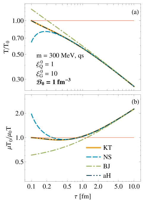
Figure 6.1: (Color online) Proper-time dependence of the effective temperature (a) and the effective baryon chemical potential (b). The exact kinetic-theory result (KT, brown solid line) is compared with the aHydro (aH, navy blue double-dot-dashed line), Navier-Stokes (NS, blue dashed line), and perfect-fluid (BJ, green dot-dashed line) results, respectively. The kinetic and aHydro calculations start with the same initial conditions. The NS and BJ calculations are adjusted to reproduce the late time behavior of the KT calculation.

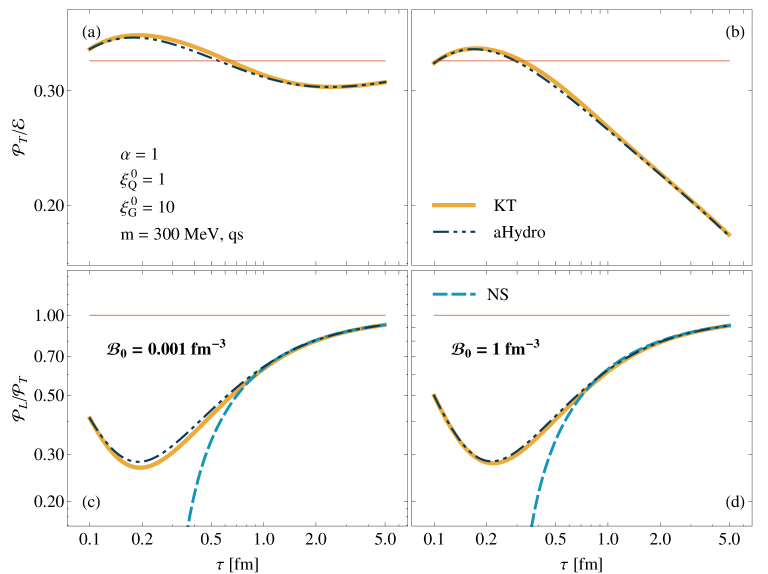
Figure 6.2: (Color online) Proper-time dependence of the ${\cal P}_{T}/{\cal E}$ (a) and ${\cal P}_{L}/{\cal P}_{T}$ (b) ratios for the initial oblate-oblate configuration. Notation the same as in Fig. 6.1.

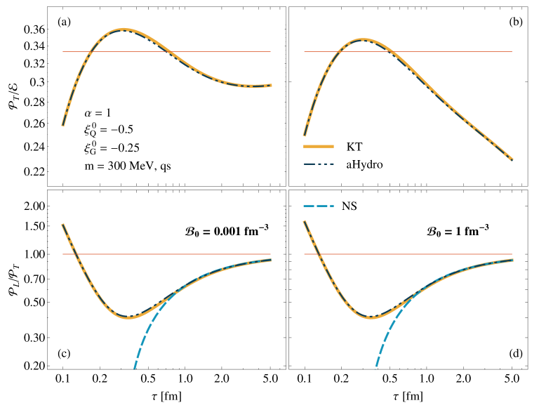
Figure 6.3: (Color online) Same as Fig. 6.2 but for the prolate-prolate initial configuration.

Equations (5.9), (5.10), (5.11), (5.15), (5.17), (5.21) and (5.22) are seven equations for seven unknown functions of the proper time: $\xi_{Q}(\tau),\Lambda_{Q}(\tau),\xi_{G}(\tau),\Lambda_{G}(\tau),\lambda(\tau),\mu(\tau)$, and $T(\tau)$. Three equations [(5.9), (5.10) and (5.15)] are algebraic but one can differentiate them with respect to proper time and use them together with the remaining four equations [(5.11), (5.17), (5.21) and (5.22)] as a system of seven ordinary differential equations of the first order. Such equations require initial values which we choose in a similar way as in [96]. The initial values of the anisotropy parameters correspond to the two options: i) $\xi_{{Q}}^{0}=1$ and $\xi_{{G}}^{0}=10$, and ii) $\xi_{{Q}}^{0}=-0.5$ and $\xi_{{G}}^{0}=-0.25$. Such values correspond to oblate-oblate and prolate-prolate initial momentum distributions of quarks and gluons, respectively. The same initial values for $\xi_{{Q}}^{0}$ and $\xi_{{G}}^{0}$ were used before also in Ref. [95]. The initial transverse momentum scales of quarks and gluons are assumed to be the same and equal to $\Lambda_{{Q}}^{0}=\Lambda_{{G}}^{0}=1$ GeV. The gluons are treated as massless, while quarks have a finite mass of 300 MeV. The initial non-equilibrium chemical potential $\lambda_{0}$ is chosen in such a way that the initial baryon number density is ${\cal B}_{0}=$ 1 fm^-3. The initial proper time is $\tau_{0}=$ 0.1 fm and the relaxation time is $\tau_{\rm eq}=$ 0.25 fm. The results shown in this section were obtained with $\alpha=0$ in Eq. (5.4). We comment on this choice below.

In Fig. 6.1 we show the proper-time dependence of the effective temperature (a) and the effective baryon chemical potential (b). The exact kinetic-theory result (KT, brown solid line) is compared with the aHydro (aH, navy blue double-dot-dashed line), Navier-Stokes (NS, blue dashed line), and perfect-fluid (BJ, green dot-dashed line) results, respectively. The kinetic and aHydro calculations start with the same initial conditions corresponding to oblate-oblate configuration defined above. The NS and BJ calculations are adjusted in such a way as to reproduce the late time behavior of the KT calculation. We observe that the KT and aHydro results agree very well during the whole evolution process. On the other hand, the NS and BJ results can reproduce the KT result only when the system approaches local equilibrium. As expected, the NS framework coincides with the KT result much earlier than BJ.

If the functions $\xi_{Q}(\tau),\Lambda_{Q}(\tau),\xi_{G}(\tau),\Lambda_{G}(\tau),\lambda(\tau),\mu(\tau)$, and $T(\tau)$ are known, we may determine the anisotropic RS distribution functions for quarks and gluons and, subsequently, use these distributions to calculate various physical observables. In Fig. 6.2 we show the proper-time dependence of the ${\cal P}_{T}/{\cal E}$ (a) and ${\cal P}_{L}/{\cal P}_{T}$ (b) ratios for the initial oblate-oblate configuration, for which the functions $T(\tau)$ and $\mu(\tau)$ are shown in Fig. 6.1. We find that aHydro reproduces very well the kinetic-theory results.

Similar, very good agreement between the KT and aHydro results is shown in Fig. 6.3 for the prolate-prolate initial conditions with $\xi_{{Q}}^{0}=-0.5$ and $\xi_{{G}}^{0}=-0.25$. Other studied cases, not shown here, also confirm very good performance of anisotropic hydrodynamics as an approximation for the kinetic theory (as far as the observables studied in this work are considered). We note that we have achieved excellent agreement with the parameter $\alpha$ set equal to zero in Eq. (5.4). Similar consistent results can be found also in the case $\alpha=1$. On the other hand, choosing a finite value of $\alpha$ from the range $0<\alpha<1$ spoils the agreement. This behavior was already observed in [95] where the case with massless particles and classical statistics was studied. Apparently, the values $0<\alpha<1$ introduce a redundant coupling between quarks and gluons, which is absent in the RTA kinetic theory.

Chapter 7 Summary

In this work, we have solved a system of coupled kinetic equations for quarks, antiquarks and gluons in the relaxation time approximation. We have generalized previous results by including the finite quark mass, the quantum statistics for both quarks and gluons, and the finite baryon number. We have compared the results of the numerical calculations with the first-order hydrodynamic calculations to demonstrate the hydrodynamization process. We have found that equalization of the longitudinal and transverse pressures takes place earlier than equalization of the average and equilibrium pressures. We have determined the shear and bulk viscosities of a mixture and find that the shear viscosity is a sum of the quark and gluon shear viscosities, while the bulk viscosity of a mixture is given by the formula known for a massive quark gas. However, the bulk viscosity depends on thermodynamic coefficients characterizing the whole mixture rather than quarks alone, which means that massless gluon do contribute to the bulk viscosity (if quarks are massive).

Appendix A Generalized thermodynamic functions

In this section, we present explicit expressions for various physical quantities such as the particle and energy densities or the transverse and longitudinal pressures. These expressions are obtained with the use of different distribution functions which not necessarily correspond to local equilibrium. Thus, we call them generalized thermodynamic functions — in local equilibrium they become standard thermodynamic functions satisfying well known thermodynamic identities. We start with the anisotropic RS distributions, as other cases can be easily worked out if the results for the RS distributions are known.

A.1 Anisotropic distributions

The forms of the generalized thermodynamic functions for anisotropic distributions (2.18) and (2.19) are given by the following integrals:

$${\cal N}^{{\rm s},{\rm a}}\equiv n_{U}^{{\rm s},{\rm a}} = k_{\rm s}\int\!dP\,\left(p\cdot U\right)f_{{\rm s},{\rm a}}\left[\vphantom{\frac{}{}}\!\,p\cdot U,\,p\cdot Z\right],$$ (A.1)

$${\cal E}^{{\rm s},{\rm a}}\equiv t_{UU}^{{\rm s},{\rm a}} = k_{\rm s}\int dP\,\left(p\cdot U\right)^{2}f_{{\rm s},{\rm a}}\left[\vphantom{\frac{}{}}\!\,p\cdot U,\,p\cdot Z\right],$$ (A.2)

$${\cal P}^{{\rm s},{\rm a}}_{T}\equiv t_{AA}^{{\rm s},{\rm a}} = k_{\rm s}\int dP\,\left(p\cdot X\right)^{2}f_{{\rm s},{\rm a}}\left[\vphantom{\frac{}{}}\!\,p\cdot U,\,p\cdot Z\right]\qquad(A\neq U,Z)$$ (A.3)

$$= k_{\rm s}\int dP\,\left(p\cdot Y\right)^{2}f_{{\rm s},{\rm a}}\left[\vphantom{\frac{}{}}\!\,p\cdot U,\,p\cdot Z\right]$$

$$= -\frac{k_{\rm s}}{2}\int dP\,(p\cdot\Delta_{T}\cdot p)f_{{\rm s},{\rm a}}\left[\vphantom{\frac{}{}}\!\,p\cdot U,\,p\cdot Z\right],$$

$${\cal P}^{{\rm s},{\rm a}}_{L}\equiv t_{ZZ}^{{\rm s},{\rm a}} = k_{\rm s}\int dP\,\left(p\cdot Z\right)^{2}f_{{\rm s},{\rm a}}\left[\vphantom{\frac{}{}}\!\,p\cdot U,\,p\cdot Z\right].$$ (A.4)

The explicit calculations lead to the following expressions for quarks and antiquarks

$${\cal N}^{{Q^{\pm}},{\rm a}} = 4\pi k_{Q}\Lambda_{Q}^{3}\tilde{{\cal H}}_{\cal N}^{+}\left(\frac{1}{\sqrt{1+\xi_{Q}}},\frac{m}{\Lambda_{Q}},\mp\frac{\lambda}{\Lambda_{Q}}\right),$$ (A.5)

$${\cal E}^{{Q^{\pm}},{\rm a}} = 2\pi k_{Q}\Lambda_{Q}^{4}\tilde{{\cal H}}^{+}\left(\frac{1}{\sqrt{1+\xi_{Q}}},\frac{m}{\Lambda_{Q}},\mp\frac{\lambda}{\Lambda_{Q}}\right),$$ (A.6)

$${\cal P}^{{Q^{\pm}},{\rm a}}_{T} = \pi k_{Q}\Lambda_{Q}^{4}\tilde{{\cal H}}_{T}^{+}\left(\frac{1}{\sqrt{1+\xi_{Q}}},\frac{m}{\Lambda_{Q}},\mp\frac{\lambda}{\Lambda_{Q}}\right),$$ (A.7)

$${\cal P}^{{Q^{\pm}},{\rm a}}_{L} = 2\pi k_{Q}\Lambda_{Q}^{4}\tilde{{\cal H}}_{L}^{+}\left(\frac{1}{\sqrt{1+\xi_{Q}}},\frac{m}{\Lambda_{Q}},\mp\frac{\lambda}{\Lambda_{Q}}\right),$$ (A.8)

where functions $\tilde{{\cal H}}\left(a,y,z\right)$ are defined by the integrals:

$$\tilde{{\cal H}}_{\cal N}^{\pm}\left(a,y,z\right) \equiv \int\limits_{0}^{\infty}r^{2}dr\,h^{{}^{\pm}}_{\rm eq}\left(\sqrt{r^{2}+y^{2}}+z\right)a,$$ (A.9)

$$\tilde{{\cal H}}^{\pm}\left(a,y,z\right) \equiv \int\limits_{0}^{\infty}r^{3}dr\,h^{{}^{\pm}}_{\rm eq}\left(\sqrt{r^{2}+y^{2}}+z\right){\cal H}_{2}\left(a,\frac{y}{r}\right),$$

$$\tilde{{\cal H}}_{T}^{\pm}\left(a,y,z\right) \equiv \int\limits_{0}^{\infty}r^{3}dr\,h^{{}^{\pm}}_{\rm eq}\left(\sqrt{r^{2}+y^{2}}+z\right){\cal H}_{2T}\left(a,\frac{y}{r}\right),$$

$$\tilde{{\cal H}}_{L}^{\pm}\left(a,y,z\right) \equiv \int\limits_{0}^{\infty}r^{3}dr\,h^{{}^{\pm}}_{\rm eq}\left(\sqrt{r^{2}+y^{2}}+z\right){\cal H}_{2L}\left(a,\frac{y}{r}\right),$$

and the functions ${\cal H}_{2}(a,b)$ were introduced in [93]:

$${\cal H}_{2}\left(a,b\right) \equiv a\int\limits_{0}^{\pi}d\varphi\,\sin\varphi\sqrt{a^{2}\cos^{2}\varphi+\sin^{2}\varphi+b^{2}},$$ (A.10)

$${\cal H}_{2T}\left(a,b\right) \equiv a\int\limits_{0}^{\pi}d\varphi\,\frac{\sin^{3}\varphi}{\sqrt{a^{2}\cos^{2}\varphi+\sin^{2}\varphi+b^{2}}},$$

$${\cal H}_{2L}\left(a,b\right) \equiv a^{3}\int\limits_{0}^{\pi}d\varphi\,\frac{\sin\varphi\,\cos^{2}\varphi}{\sqrt{a^{2}\cos^{2}\varphi+\sin^{2}\varphi+b^{2}}}.$$

The integrals in (A.10) are analytic and give [93]:

$${\cal H}_{2}(a,b)\!\! = \!\!\frac{a}{\sqrt{a^{2}-1}}\left((1+b^{2})\tanh^{-1}\sqrt{\frac{a^{2}-1}{a^{2}+b^{2}}}+\sqrt{(a^{2}-1)(a^{2}+b^{2})}\,\right),$$ (A.11)

$${\cal H}_{2T}(a,b)\!\! = \!\!\frac{a}{(a^{2}-1)^{3/2}}\left(\left(b^{2}+2a^{2}-1\right)\tanh^{-1}\sqrt{\frac{a^{2}-1}{a^{2}+b^{2}}}-\sqrt{(a^{2}-1)(a^{2}+b^{2})}\right),$$ (A.12)

$${\cal H}_{2L}(a,b)\!\! = \!\!\frac{a^{3}}{(a^{2}-1)^{3/2}}\left(-(1+b^{2})\tanh^{-1}\sqrt{\frac{a^{2}-1}{a^{2}+b^{2}}}+\sqrt{(a^{2}-1)(a^{2}+b^{2})}\,\,\right).$$ (A.13)

With $b=0$ the functions ${\cal H}_{2}(a,b)$, ${\cal H}_{2T}(a,b)$ and ${\cal H}_{2L}(a,b)$ reduce to the functions ${\cal H}(a)$, ${\cal H}_{T}(a)$ and ${\cal H}_{L}(a)$ used in [24, 25].

For gluons one has:

$${\cal N}^{{G},{\rm a}} = 4\pi k_{G}\Lambda_{G}^{3}\tilde{{\cal H}}_{\cal N}^{-}\left(\frac{1}{\sqrt{1+\xi_{G}}},0,0\right)=8\pi\zeta(3)k_{G}\Lambda_{G}^{3}\frac{1}{\sqrt{1+\xi_{G}}},$$ (A.14)

$${\cal E}^{{G},{\rm a}} = 2\pi k_{G}\Lambda_{G}^{4}\tilde{{\cal H}}^{-}\left(\frac{1}{\sqrt{1+\xi_{G}}},0,0\right)=\frac{2\pi^{5}}{15}k_{G}\Lambda_{G}^{4}{\cal H}\left(\frac{1}{\sqrt{1+\xi_{G}}}\right),$$ (A.15)

$${\cal P}^{{G},{\rm a}}_{T} = \pi k_{G}\Lambda_{G}^{4}\tilde{{\cal H}}_{T}^{-}\left(\frac{1}{\sqrt{1+\xi_{G}}},0,0\right)=\frac{\pi^{5}}{15}k_{G}\Lambda_{G}^{4}{\cal H}_{T}\left(\frac{1}{\sqrt{1+\xi_{G}}}\right),$$ (A.16)

$${\cal P}^{{G},{\rm a}}_{L} = 2\pi k_{G}\Lambda_{G}^{4}\tilde{{\cal H}}_{L}^{-}\left(\frac{1}{\sqrt{1+\xi_{G}}},0,0\right)=\frac{2\pi^{5}}{15}k_{G}\Lambda_{G}^{4}{\cal H}_{L}\left(\frac{1}{\sqrt{1+\xi_{G}}}\right),$$ (A.17)

where $\zeta$ is the Riemann zeta function . The expressions on the right-hand sides of Eqs. (A.14)–(A.17) hold for the Bose-Einstein statistics. Note that in the case of massless gluons the integrals (A.10) are done for $b=0$ and can be factorized in Eqs. (A.9). The functions ${\cal H}$, ${\cal H}_{T}$, and ${\cal H}_{L}$ in Eqs. (A.15)–(A.17) are defined in [24, 25].

It is useful to notice that the functions ${\cal H}_{2}$ and ${\cal H}_{2L}$ are related by the expression

$$\frac{\partial{\cal H}_{2}\left(a,b\right)}{\partial a}=\frac{{\cal H}_{2}\left(a,b\right)+{\cal H}_{2L}\left(a,b\right)}{a},$$ (A.18)

hence, we also have

$$\frac{\partial\tilde{{\cal H}}^{\pm}\left(a,y,z\right)}{\partial a}=\frac{\tilde{{\cal H}}^{\pm}\left(a,y,z\right)+\tilde{{\cal H}}^{\pm}\left(a,y,z\right)}{a}.$$ (A.19)

We can use (A.19) to derive (3.33) from (3.31).

We close this section with the formula for the baryon number density valid for anisotropic RS systems

$${\cal B}^{\rm a} = \frac{{\cal N}^{{Q^{+}},{\rm a}}-{\cal N}^{{Q^{-}},{\rm a}}}{3}=\frac{16\pi k_{Q}\Lambda_{Q}^{3}}{3\sqrt{1+\xi_{Q}}}\sinh\left(\frac{\lambda}{\Lambda_{Q}}\right)\,{\cal H}_{\cal B}\left(\frac{m}{\Lambda_{Q}},\frac{\lambda}{\Lambda_{Q}}\right),$$ (A.20)

where

$${\cal H}_{\cal B}\left(y,z\right) \equiv \frac{1}{4}\int\limits_{0}^{\infty}r^{2}dr\left[\frac{1}{\cosh\sqrt{r^{2}+y^{2}}+\cosh z}\right].$$ (A.21)

A.2 Isotropic distributions

The forms of the thermodynamic functions for the isotropic equilibrium state are commonly known, nevertheless, we quote them here for completeness. They are given by the formulas

$${\cal N}^{{\rm s},{\rm eq}}\equiv n_{U}^{{\rm s},{\rm eq}} = k_{\rm s}\int\!dP\,\left(p\cdot U\right)f_{{\rm s},{\rm eq}}(p\cdot U),$$ (A.22)

$${\cal E}^{{\rm s},{\rm eq}}\equiv t_{UU}^{{\rm s},{\rm eq}} = k_{\rm s}\int dP\,\left(p\cdot U\right)^{2}f_{{\rm s},{\rm eq}}(p\cdot U),$$ (A.23)

$${\cal P}^{{\rm s},{\rm eq}}\equiv t_{AA}^{{\rm s},{\rm eq}} = k_{\rm s}\int\!dP\,\left(p\cdot A\right)^{2}f_{{\rm s},{\rm eq}}(p\cdot U)$$ (A.24)

$$= -\frac{k_{\rm s}}{3}\int\!dP\,(p\cdot\Delta\cdot p)f_{{\rm s},{\rm eq}}(p\cdot U),\quad(A\neq U).$$

The explicit expressions for quarks and antiquarks may be obtained from Eqs. (A.5)–(A.8) as a special case of $\xi_{\rm s}\to 0$, $\Lambda_{\rm s}\to T$, and $\lambda_{\rm s}\to\mu$,

$${\cal N}^{{Q^{\pm}},{\rm eq}}\!\! = \!\!4\pi k_{Q}T^{3}\tilde{{\cal H}}_{\cal N}^{+}\left(1,\frac{m}{T},\mp\frac{\mu}{T}\right),$$ (A.25)

$${\cal E}^{{Q^{\pm}},{\rm eq}}\!\! = \!\!2\pi k_{Q}T^{4}\tilde{{\cal H}}^{+}\left(1,\frac{m}{T},\mp\frac{\mu}{T}\right),$$ (A.26)

$${\cal P}^{{Q^{\pm}},{\rm eq}}_{T}\!\! = \!\!\pi k_{Q}T^{4}\tilde{{\cal H}}_{T}^{+}\left(1,\frac{m}{T},\mp\frac{\mu}{T}\right),$$ (A.27)

$${\cal P}^{{Q^{\pm}},{\rm eq}}_{L}\!\! = \!\!2\pi k_{Q}T^{4}\tilde{{\cal H}}_{L}^{+}\left(1,\frac{m}{T},\mp\frac{\mu}{T}\right).$$ (A.28)

Note that ${\cal H}_{2L}(1,b)=2/\left(3\sqrt{1+b^{2}}\right)$ and ${\cal H}_{2T}(1,b)=4/\left(3\sqrt{1+b^{2}}\right)$ which means that ${\cal P}^{{Q^{\pm}},{\rm eq}}_{T}={\cal P}^{{Q^{\pm}},{\rm eq}}_{L}\equiv{\cal P}^{{Q^{\pm}},{\rm eq}}$, as expected for the isotropic state. Analogous results may be obtained for gluons

$${\cal N}^{{G},{\rm eq}}\!\! = \!\!4\pi k_{G}T^{3}\tilde{{\cal H}}_{\cal N}^{-}\left(1,0,0\right)=8\pi\zeta(3)k_{G}T^{3},$$ (A.29)

$${\cal E}^{{G},{\rm eq}}\!\! = \!\!2\pi k_{G}T^{4}\tilde{{\cal H}}^{-}\left(1,0,0\right)=\frac{4\pi^{5}}{15}k_{G}T^{4},$$ (A.30)

$${\cal P}^{{G},{\rm eq}}_{T}\!\! = \!\!\pi k_{G}T^{4}\tilde{{\cal H}}_{T}^{-}\left(1,0,0\right)=\frac{4\pi^{5}}{45}k_{G}T^{4},$$ (A.31)

$${\cal P}^{{G},{\rm eq}}_{L}\!\! = \!\!2\pi k_{G}T^{4}\tilde{{\cal H}}_{L}^{-}\left(1,0,0\right)=\frac{4\pi^{5}}{45}k_{G}T^{4},$$ (A.32)

where to get the last expressions on the right-hand sides we again assumed the Bose-Einstein statistics. Here, similarly as for quarks ${\cal P}^{{G},{\rm eq}}_{T}={\cal P}^{{G},{\rm eq}}_{L}\equiv{\cal P}^{{G},{\rm eq}}$. Similarly to the anisotropic case the baryon number density is

$${\cal B}^{\rm eq} = \frac{{\cal N}^{{Q^{+}},{\rm eq}}-{\cal N}^{{Q^{-}},{\rm eq}}}{3}=\frac{16\pi k_{Q}T^{3}}{3}\sinh\left(\frac{\mu}{T}\right)\,{\cal H}_{\cal B}\left(\frac{m}{T},\frac{\mu}{T}\right).$$ (A.33)

with ${\cal H}_{\cal B}\left(y,z\right)$ given in Eq. (A.21).

A.3 Exact distributions

For the solutions of Eqs. (3.6) of the form (3.10) the thermodynamic variables have the forms

$${\cal N}^{{\rm s}} = k_{\rm s}\int\!dP\,\left(p\cdot U\right)f_{{\rm s}}\left[\vphantom{\frac{}{}}\!\,p\cdot U,p\cdot Z\right],$$

$${\cal E}^{{\rm s}} = k_{\rm s}\int dP\,\left(p\cdot U\right)^{2}f_{{\rm s}}\left[\vphantom{\frac{}{}}\!\,p\cdot U,p\cdot Z\right],$$ (A.34)

$${\cal P}^{{\rm s}}_{T} = k_{\rm s}\int dP\,\left(p\cdot A\right)^{2}f_{{\rm s}}\left[\vphantom{\frac{}{}}\!\,p\cdot U,p\cdot Z\right]\qquad(A\neq U,Z),$$

$${\cal P}^{{\rm s}}_{L} = k_{\rm s}\int dP\,\left(p\cdot Z\right)^{2}f_{{\rm s}}\left[\vphantom{\frac{}{}}\!\,p\cdot U,p\cdot Z\right].$$

Using the above definitions and repeating the calculation from Sec. A.1, gives

$${\cal N}^{{Q^{\pm}}} = 4\pi k_{Q}\left[\left(\Lambda_{Q}^{0}\right)^{3}\tilde{{\cal H}}_{\cal N}^{+}\left(\frac{\tau_{0}}{\tau\sqrt{1+\xi_{Q}^{0}}},\frac{m}{\Lambda_{Q}^{0}},\mp\frac{\lambda^{0}}{\Lambda_{Q}^{0}}\right)D(\tau,\tau_{0})\right.$$

$$\left.\hskip 142.26378pt+\int\limits_{\tau_{0}}^{\tau}\frac{d\tau^{\prime}}{\tau_{\rm eq}^{\prime}}\ D(\tau,\tau^{\prime})\left(T^{\prime}\right)^{3}\tilde{{\cal H}}_{\cal N}^{+}\left(\frac{\tau^{\prime}}{\tau},\frac{m}{T^{\prime}},\mp\frac{\mu^{\prime}}{T^{\prime}}\right)\right],$$

$${\cal E}^{{Q^{\pm}}} = 2\pi k_{Q}\left[\left(\Lambda_{Q}^{0}\right)^{4}\tilde{{\cal H}}^{+}\left(\frac{\tau_{0}}{\tau\sqrt{1+\xi_{Q}^{0}}},\frac{m}{\Lambda_{Q}^{0}},\mp\frac{\lambda^{0}}{\Lambda_{Q}^{0}}\right)D(\tau,\tau_{0})\right.$$

$$\left.\hskip 142.26378pt+\int\limits_{\tau_{0}}^{\tau}\frac{d\tau^{\prime}}{\tau_{\rm eq}^{\prime}}\ D(\tau,\tau^{\prime})\left(T^{\prime}\right)^{4}\tilde{{\cal H}}^{+}\left(\frac{\tau^{\prime}}{\tau},\frac{m}{T^{\prime}},\mp\frac{\mu^{\prime}}{T^{\prime}}\right)\right],$$

$${\cal P}^{{Q^{\pm}}}_{T} = \pi k_{Q}\left[\left(\Lambda_{Q}^{0}\right)^{4}\tilde{{\cal H}}_{T}^{+}\left(\frac{\tau_{0}}{\tau\sqrt{1+\xi_{Q}^{0}}},\frac{m}{\Lambda_{Q}^{0}},\mp\frac{\lambda^{0}}{\Lambda_{Q}^{0}}\right)D(\tau,\tau_{0})\right.$$

$$\left.\hskip 142.26378pt+\int\limits_{\tau_{0}}^{\tau}\frac{d\tau^{\prime}}{\tau_{\rm eq}^{\prime}}\ D(\tau,\tau^{\prime})\left(T^{\prime}\right)^{4}\tilde{{\cal H}}_{T}^{+}\left(\frac{\tau^{\prime}}{\tau},\frac{m}{T^{\prime}},\mp\frac{\mu^{\prime}}{T^{\prime}}\right)\right],$$

$${\cal P}^{{Q^{\pm}}}_{L} = 2\pi k_{Q}\left[\left(\Lambda_{Q}^{0}\right)^{4}\tilde{{\cal H}}_{L}^{+}\left(\frac{\tau_{0}}{\tau\sqrt{1+\xi_{Q}^{0}}},\frac{m}{\Lambda_{Q}^{0}},\mp\frac{\lambda^{0}}{\Lambda_{Q}^{0}}\right)D(\tau,\tau_{0})\right.$$

$$\left.\hskip 142.26378pt+\int\limits_{\tau_{0}}^{\tau}\frac{d\tau^{\prime}}{\tau_{\rm eq}^{\prime}}\ D(\tau,\tau^{\prime})\left(T^{\prime}\right)^{4}\tilde{{\cal H}}_{L}^{+}\left(\frac{\tau^{\prime}}{\tau},\frac{m}{T^{\prime}},\mp\frac{\mu^{\prime}}{T^{\prime}}\right)\right],$$

for quarks and

$${\cal N}^{{G}} = 4\pi k_{G}\left[\left(\Lambda_{G}^{0}\right)^{3}\tilde{{\cal H}}_{\cal N}^{-}\left(\frac{\tau_{0}}{\tau\sqrt{1+\xi_{G}^{0}}},0,0\right)D(\tau,\tau_{0})+\int\limits_{\tau_{0}}^{\tau}\frac{d\tau^{\prime}}{\tau_{\rm eq}^{\prime}}\ D(\tau,\tau^{\prime})\left(T^{\prime}\right)^{3}\tilde{{\cal H}}_{\cal N}^{-}\left(\frac{\tau^{\prime}}{\tau},0,0\right)\right],$$

$${\cal E}^{{G}} = 2\pi k_{G}\left[\left(\Lambda_{G}^{0}\right)^{4}\tilde{{\cal H}}^{-}\left(\frac{\tau_{0}}{\tau\sqrt{1+\xi_{G}^{0}}},0,0\right)D(\tau,\tau_{0})+\int\limits_{\tau_{0}}^{\tau}\frac{d\tau^{\prime}}{\tau_{\rm eq}^{\prime}}\ D(\tau,\tau^{\prime})\left(T^{\prime}\right)^{4}\tilde{{\cal H}}^{-}\left(\frac{\tau^{\prime}}{\tau},0,0\right)\right],$$

$${\cal P}^{{G}}_{T} = \pi k_{G}\left[\left(\Lambda_{G}^{0}\right)^{4}\tilde{{\cal H}}_{T}^{-}\left(\frac{\tau_{0}}{\tau\sqrt{1+\xi_{G}^{0}}},0,0\right)D(\tau,\tau_{0})+\int\limits_{\tau_{0}}^{\tau}\frac{d\tau^{\prime}}{\tau_{\rm eq}^{\prime}}\ D(\tau,\tau^{\prime})\left(T^{\prime}\right)^{4}\tilde{{\cal H}}_{T}^{-}\left(\frac{\tau^{\prime}}{\tau},0,0\right)\right],$$

$${\cal P}^{{G}}_{L} = 2\pi k_{G}\left[\left(\Lambda_{G}^{0}\right)^{4}\tilde{{\cal H}}_{L}^{-}\left(\frac{\tau_{0}}{\tau\sqrt{1+\xi_{G}^{0}}},0,0\right)D(\tau,\tau_{0})+\int\limits_{\tau_{0}}^{\tau}\frac{d\tau^{\prime}}{\tau_{\rm eq}^{\prime}}\ D(\tau,\tau^{\prime})\left(T^{\prime}\right)^{4}\tilde{{\cal H}}_{L}^{-}\left(\frac{\tau^{\prime}}{\tau},0,0\right)\right],$$

for gluons. We define the baryon number density for the exact solution of the kinetic equation as follows

$${\cal B} = \frac{16\pi k_{Q}}{3}\left[\frac{\tau_{0}\left(\Lambda_{Q}^{0}\right)^{3}}{\tau\sqrt{1+\xi_{Q}^{0}}}\sinh\left(\frac{\lambda^{0}}{\Lambda_{Q}^{0}}\right)\,{\cal H}_{\cal B}\left(\frac{m}{\Lambda_{Q}^{0}},\frac{\lambda^{0}}{\Lambda_{Q}^{0}}\right)D(\tau,\tau_{0})\right.$$

$$\left.\hskip 142.26378pt+\int\limits_{\tau_{0}}^{\tau}\frac{d\tau^{\prime}}{\tau_{\rm eq}^{\prime}}\ D(\tau,\tau^{\prime})\frac{\tau^{\prime}\left(T^{\prime}\right)^{3}}{\tau}\sinh\left(\frac{\mu^{\prime}}{T^{\prime}}\right)\,{\cal H}_{\cal B}\left(\frac{m}{T^{\prime}},\frac{\mu^{\prime}}{T^{\prime}}\right)\right].$$

Appendix B Second moments of the distribution function

The second moment of the distribution function is expressed by the momentum integral

$$\Theta_{\rm s}^{\lambda\mu\nu}(x) = k_{\rm s}\int\!dP\,p^{\lambda}p^{\mu}p^{\nu}f_{\rm s}(x,p).$$ (B.1)

The latter may be decomposed in the tensorial basis contructed using the tensor products of the basis four-vectors $A^{\mu}_{(\alpha)}=\{U^{\mu},X^{\mu},Y^{\mu},Z^{\mu}\}$,

$$\Theta_{\rm s}^{\lambda\mu\nu}(x) = \sum_{A,B,C}c_{ABC}^{{\rm s}}A^{\lambda}B^{\mu}C^{\nu},$$ (B.2)

where the coefficients $c_{ABC}^{{\rm s}}$ are defined through the expression

$$c_{ABC}^{{\rm s}} = A_{\lambda}^{\,}B_{\mu}^{\,}C_{\nu}^{\,}\Theta_{\rm s}^{\lambda\mu\nu}(x)\,A^{2}B^{2}C^{2}.$$ (B.3)

Using Eq. (B.1) one thus has

$$c_{ABC}^{{\rm s}} = k_{\rm s}\int\!dP\,\left(p\cdot A\right)\left(p\cdot B\right)\left(p\cdot C\right)A^{2}B^{2}C^{2}f_{\rm s}(x,p).$$ (B.4)

For the distribution functions specified in Eqs. (2.14) and (2.15) and Eqs. (2.18) and (2.19), due to the symmetry arguments, the only non-vanishing coefficients $c_{ABC}^{{\rm s}}$ out of those in Eq. (B.4) are the ones with an even number of each spatial index of $p^{\mu}$ which means that Eq. (B.2) may be expressed as follows

$$\Theta_{\rm s}^{\lambda\mu\nu}(x) = c_{UUU}^{{\rm s}}U^{\lambda}U^{\mu}U^{\nu}+\sum_{A}c_{UAA}^{{\rm s}}(U^{\lambda}A^{\mu}A^{\nu}+A^{\lambda}U^{\mu}A^{\nu}+A^{\lambda}A^{\mu}U^{\nu}).$$ (B.5)

B.1 Anisotropic distributions

For the anisotropic distribution functions, one may exploit the SO(2) symmetry of the Eqs. (2.18)-(2.19) in transverse momentum plane and write

$$\Theta_{{\rm s},{\rm a}}^{\lambda\mu\nu} = \vartheta_{U}^{{\rm s},{\rm a}}\,U^{\lambda}U^{\mu}U^{\nu}$$ (B.6)

$$- \,\vartheta_{T}^{{\rm s},{\rm a}}\,\left(U^{\lambda}\Delta^{\mu\nu}_{T}+U^{\mu}\Delta^{\lambda\nu}_{T}+U^{\nu}\Delta^{\lambda\mu}_{T}\right)$$ (B.7)

$$+ \,\vartheta_{L}^{{\rm s},{\rm a}}\,\left(U^{\lambda}Z^{\mu}Z^{\nu}+U^{\mu}Z^{\lambda}Z^{\nu}+U^{\nu}Z^{\lambda}Z^{\mu}\right),$$ (B.8)

where $\vartheta_{U}^{{\rm s},{\rm a}}\equiv c_{UUU}^{{\rm s},{\rm a}}$, $\vartheta_{T}^{{\rm s},{\rm a}}\equiv c_{UXX}^{{\rm s},{\rm a}}=c_{UYY}^{{\rm s},{\rm a}}$, and $\vartheta_{L}^{{\rm s},{\rm a}}\equiv c_{UZZ}^{{\rm s},{\rm a}}$.

For quarks explicit calculation gives

$$\vartheta_{U}^{{Q^{\pm}},{\rm a}} = \frac{4\pi k_{Q}\Lambda_{Q}^{5}}{3}\frac{(3+2\xi_{Q})}{(1+\xi_{Q})^{3/2}}\tilde{{\cal H}}_{\vartheta}^{+}\left(\frac{m}{\Lambda_{Q}},\mp\frac{\lambda}{\Lambda_{Q}}\right)+m^{2}{\cal N}^{{Q^{\pm}},{\rm a}},$$ (B.9)

$$\vartheta_{T}^{{Q^{\pm}},{\rm a}} = \frac{4\pi k_{Q}\Lambda_{Q}^{5}}{3}\frac{1}{\sqrt{1+\xi_{Q}}}\tilde{{\cal H}}_{\vartheta}^{+}\left(\frac{m}{\Lambda_{Q}},\mp\frac{\lambda}{\Lambda_{Q}}\right),$$ (B.10)

$$\vartheta_{L}^{{Q^{\pm}},{\rm a}} = \frac{4\pi k_{Q}\Lambda_{Q}^{5}}{3}\frac{1}{(1+\xi_{Q})^{3/2}}\tilde{{\cal H}}_{\vartheta}^{+}\left(\frac{m}{\Lambda_{Q}},\mp\frac{\lambda}{\Lambda_{Q}}\right),$$ (B.11)

where

$$\tilde{{\cal H}}_{\vartheta}^{\pm}\left(y,z\right) \equiv \int\limits_{0}^{\infty}r^{4}dr\,h^{{}^{\pm}}_{\rm eq}\left(\sqrt{r^{2}+y^{2}}+z\right).$$ (B.12)

Analogous expressions hold for gluons where the integral in Eq. (B.12) yields $\tilde{{\cal H}}_{\vartheta}^{\pm}\left(0,0\right)=24\zeta(5)$ with $\zeta$ being the Riemann zeta function.

B.2 Isotropic distributions

For the equilibrium distribution functions the SO(3) symmetry of the Eqs. (2.14)-(2.15) in the momentum space allows one to write

$$\Theta_{{\rm s},{\rm eq}}^{\lambda\mu\nu} = \vartheta_{U}^{{\rm s},{\rm eq}}\,U^{\lambda}U^{\mu}U^{\nu}-\vartheta^{{\rm s},{\rm eq}}\,\left(U^{\lambda}\Delta^{\mu\nu}+U^{\mu}\Delta^{\lambda\nu}+U^{\nu}\Delta^{\lambda\mu}\right)$$ (B.13)

where $\vartheta_{U}^{{\rm s},{\rm eq}}\equiv c_{UUU}^{{\rm s},{\rm a}}$, and $\vartheta^{{\rm s},{\rm eq}}\equiv c_{UXX}^{{\rm s},{\rm eq}}=c_{UYY}^{{\rm s},{\rm eq}}=c_{UZZ}^{{\rm s},{\rm eq}}$ are obtained from expressions (B.9)-(B.11) taking the limit $\xi_{s}\to 0$ where $\Lambda_{s}\to T$.

Appendix C Navier-Stokes hydrodynamics

The results of our kinetic-theory calculations are compared with the viscous hydrodynamic results obtained by solving the Navier-Stokes (NS) hydrodynamic equations. The latter have the form

$$\frac{d}{d\tau}\left({\cal E}^{{Q},{\rm eq}}+{\cal E}^{{G},{\rm eq}}\right) = -\frac{{\cal E}^{{Q},{\rm eq}}+{\cal E}^{{G},{\rm eq}}+{\cal P}^{{Q},{\rm eq}}+{\cal P}^{{G},{\rm eq}}+\Pi_{\rm NS}-\pi_{\rm NS}}{\tau},$$ (C.1)

$$\frac{d{\cal B}^{{\rm eq}}}{d\tau}+\frac{{\cal B}^{{\rm eq}}}{\tau} = 0.$$ (C.2)

Here ${\cal E}^{{Q},{\rm eq}}={\cal E}^{{Q^{+}},{\rm eq}}+{\cal E}^{{Q^{-}},{\rm eq}}$ is the equilibrium energy density of quarks and antiquarks, ${\cal P}^{{Q},{\rm eq}}={\cal P}^{{Q^{+}},{\rm eq}}+{\cal P}^{{Q^{-}},{\rm eq}}$ is the equilibrium pressure of quarks and antiquarks, $\Pi_{\rm NS}$ is the bulk pressure, and $\pi_{\rm NS}$ is the shear pressure (both used in the close-to-equilibrium limit). All the functions appearing in (C.1) and (C.2) depend on $T$ and $\mu$, hence Eqs. (C.1) and (C.2) are two coupled equations that can be used to determine $T(\tau)$ and $\mu(\tau)$. One can easily notice that Eq. (C.1) may be written in the form of Eq. (3.33) once we identify

$${\cal P}_{L} = {\cal P}^{\rm eq}-\pi_{\rm NS}+\Pi_{\rm NS},$$ (C.3)

$${\cal P}_{T} = {\cal P}^{\rm eq}+\frac{1}{2}\pi_{\rm NS}+\Pi_{\rm NS},$$

where ${\cal P}^{{\rm eq}}={\cal P}^{{Q},{\rm eq}}+{\cal P}^{{G},{\rm eq}}$. Within NS approach, the shear and bulk pressures are expressed by the kinetic coefficients $\eta$ and $\zeta$,

$$\pi_{\rm NS}=\frac{4\eta}{3\tau}=\frac{4(\eta_{Q}+\eta_{G})}{3\tau},$$ (C.4)

$$\Pi_{\rm NS}=-\frac{\zeta}{\tau}.$$ (C.5)

The expressions for $\eta_{Q}$, $\eta_{G}$, and $\zeta$ are given by Eqs. (4.3), (4.4), and (4.7).

For the moment let us denote $T(\tau)$ and $\mu(\tau)$ obtained from the kinetic theory as $T_{\rm KT}(\tau)$ and $\mu_{\rm KT}(\tau)$, while those obtained from the NS hydrodynamics as $T_{\rm NS}(\tau)$ and $\mu_{\rm NS}(\tau)$. We expect that $T_{\rm KT}(\tau)$ and $\mu_{\rm KT}(\tau)$ agree well with $T_{\rm NS}(\tau)$ and $\mu_{\rm NS}(\tau)$ in the late stages of the evolution when the system approaches local equilibrium. To check this behavior we choose such initial conditions for hydrodynamic equations (C.1) and (C.2) that for the final time $\tau=\tau_{f}$ we match the temperature and chemical potential in the two approaches: $T_{\rm NS}(\tau_{f})=T_{\rm KT}(\tau_{f})$, $\mu_{\rm NS}(\tau_{f})=\mu_{\rm KT}(\tau_{f})$. Then, we check if the functions $T_{\rm NS}(\tau)$ and $\mu_{\rm NS}(\tau)$ smoothly approach $T_{\rm KT}(\tau)$ and $\mu_{\rm KT}(\tau)$ if $\tau\to\tau_{f}$. By neglecting the bulk and shear pressures in (C.1) we can also make a comparison with perfect fluid hydrodynamics and check if the system approaches local equilibrium.

Appendix D Shear and bulk viscosities for mixtures

In this section, we present details of our method used to calculate the shear and bulk viscosity coefficients for a quark-gluon mixture. We follow the treatment of Refs. [132, 133], where the bulk viscosity was obtained for the Gribov-Zwanziger plasma. Analyzing a boost-invariant system, we deal with a simple structure of hydrodynamic equations, which facilitates the calculations.

D.1 Landau matching conditions in the case of boost invariant geometry

In the first order of the gradient expansion, the non-equilibrium corrections to the equilibrium distribution function have the form

$$\delta f_{Q^{\pm}}=-\tau_{\rm eq}\frac{\partial f_{{Q^{\pm}},{\rm eq}}}{\partial\tau},\quad\delta f_{G}=-\tau_{\rm eq}\frac{\partial f_{{G},{\rm eq}}}{\partial\tau}.$$ (D.1)

Using the form of $f_{{Q^{\pm}},{\rm eq}}$ and $f_{{G},{\rm eq}}$ for boost-invariant geometry (3.7)–(3.8) we find

$$\delta f_{Q^{\pm}} = -\tau_{\rm eq}f_{{Q^{\pm}},{\rm eq}}\left(1-f_{{Q^{\pm}},{\rm eq}}\right)\left[\frac{w^{2}}{v\tau^{2}T}\pm\frac{d\mu}{Td\tau}+\left(\frac{v}{\tau}\mp\mu\right)\frac{d\ln T}{Td\tau}\right],$$ (D.2)

$$\delta f_{G} = -\tau_{\rm eq}f_{{G},{\rm eq}}\left(1+f_{{G},{\rm eq}}\right)\left[\frac{w^{2}}{v\tau^{2}T}+\frac{v}{\tau}\frac{d\ln T}{Td\tau}\right].$$ (D.3)

The Landau matching conditions for the energy and momentum read

$$\int\frac{dwd^{2}p_{T}}{v}\,\frac{v^{2}}{\tau^{2}}\left[k_{Q}\left(\delta f_{Q^{+}}+\delta f_{Q^{-}}\right)+k_{G}\delta f_{G}\right]=0,$$ (D.4)

$$\int\frac{dwd^{2}p_{T}}{v}\,\frac{v^{2}}{3\tau^{2}}\left[k_{Q}\left(\delta f_{Q^{+}}-\delta f_{Q^{-}}\right)\right]=0.$$ (D.5)

Using (D.2) and (D.3) we rewrite (D.4) and (D.5) as

$$\int\frac{dwd^{2}p_{T}}{v}\,\frac{v^{2}}{\tau^{2}}\,f_{3S}\,\frac{w^{2}}{v\tau^{2}T}+\int\frac{dwd^{2}p_{T}}{v}\,\frac{v^{2}}{\tau^{2}}\,f_{2D}\,\frac{d\mu}{Td\tau}$$

$$+\int\frac{dwd^{2}p_{T}}{v}\,\frac{v^{2}}{\tau^{2}}\,f_{3S}\,\frac{v}{T\tau}\,\frac{d\ln T}{d\tau}-\int\frac{dwd^{2}p_{T}}{v}\,\frac{v^{2}}{\tau^{2}}\,f_{2D}\,\frac{\mu}{T}\frac{d\ln T}{d\tau}=0$$ (D.6)

and

$$\int\frac{dwd^{2}p_{T}}{v}\,\frac{v^{2}}{\tau^{2}}\,f_{2D}\,\frac{w^{2}}{v\tau^{2}T}+\int\frac{dwd^{2}p_{T}}{v}\,\frac{v^{2}}{\tau^{2}}\,f_{2S}\,\frac{d\mu}{Td\tau}$$

$$+\int\frac{dwd^{2}p_{T}}{v}\,\frac{v^{2}}{\tau^{2}}\,f_{2D}\,\frac{v}{T\tau}\,\frac{d\ln T}{d\tau}-\int\frac{dwd^{2}p_{T}}{v}\,\frac{v^{2}}{\tau^{2}}\,f_{2S}\,\frac{\mu}{T}\frac{d\ln T}{d\tau}=0,$$ (D.7)

where

$$f_{3S} = k_{Q}\left[f_{{Q^{+}},{\rm eq}}\left(1-f_{{Q^{+}},{\rm eq}}\right)+f_{{Q^{-}},{\rm eq}}\left(1-f_{{Q^{-}},{\rm eq}}\right)\right]+k_{G}f_{{G},{\rm eq}}\left(1+f_{{G},{\rm eq}}\right),$$

$$f_{2S} = k_{Q}\left[f_{{Q^{+}},{\rm eq}}\left(1-f_{{Q^{+}},{\rm eq}}\right)+f_{{Q^{-}},{\rm eq}}\left(1-f_{{Q^{-}},{\rm eq}}\right)\right],$$

$$f_{2D} = k_{Q}\left[f_{{Q^{+}},{\rm eq}}\left(1-f_{{Q^{+}},{\rm eq}}\right)-f_{{Q^{-}},{\rm eq}}\left(1-f_{{Q^{-}},{\rm eq}}\right)\right].$$ (D.8)

By introducing the “averaged” values defined as

$$\langle...\rangle_{\alpha}\equiv\int\frac{dwd^{2}p_{T}}{v}...f_{\alpha},$$ (D.9)

where $\alpha=3S,2S,2D$, we rewrite (D.6) and (D.7) in the compact form

$$\langle w^{2}\rangle_{3S}+\langle v^{2}\rangle_{3S}\frac{d\ln T}{d\ln\tau}+\langle v\rangle_{2D}\tau^{2}T\frac{d}{d\tau}\left(\frac{\mu}{T}\right) = 0,$$

$$\langle\frac{w^{2}}{v}\rangle_{2D}+\langle v\rangle_{2D}\frac{d\ln T}{d\ln\tau}+\langle 1\rangle_{2S}\tau^{2}T\frac{d}{d\tau}\left(\frac{\mu}{T}\right) = 0.$$ (D.10)

To proceed further it is convenient to introduce the notation

$$A=\langle w^{2}\rangle_{3S},\,\,B=\langle v^{2}\rangle_{3S},\,\,C=\langle v\rangle_{2D},\,\,D=\langle\frac{w^{2}}{v}\rangle_{2D},\,\,E=\langle 1\rangle_{2S}.$$ (D.11)

Then, we find the proper-time derivatives of $T$ and $\mu/T$ expressed by the coefficients (D.11)

$$\frac{d\ln T}{d\ln\tau}=\frac{AE-CD}{C^{2}-BE},\quad\tau^{2}T\frac{d}{d\tau}\left(\frac{\mu}{T}\right)=\frac{DB-AC}{C^{2}-BE}.$$ (D.12)

The coefficients (D.11) can be used also to express various thermodynamic derivatives. After straightforward calculations, where $T$ and $\mu$ are treated as independent thermodynamic variables, we find

$$\frac{\partial{\cal P}^{\rm eq}}{\partial T} = \frac{\partial{\cal P}^{{Q^{+}},\rm eq}}{\partial T}+\frac{\partial{\cal P}^{{Q^{-}},\rm eq}}{\partial T}+\frac{\partial{\cal P}^{{G},\rm eq}}{\partial T}=\frac{A}{\tau^{3}T^{2}}-\frac{D\mu}{\tau^{2}T^{2}},$$

$$\frac{\partial{\cal P}^{\rm eq}}{\partial\mu} = \frac{\partial{\cal P}^{{Q^{+}},\rm eq}}{\partial\mu}+\frac{\partial{\cal P}^{{Q^{-}},\rm eq}}{\partial\mu}=\frac{D}{\tau^{2}T},$$

$$\frac{\partial{\cal E}^{\rm eq}}{\partial T} = \frac{\partial{\cal E}^{{Q^{+}},\rm eq}}{\partial T}+\frac{\partial{\cal E}^{{Q^{-}},\rm eq}}{\partial T}+\frac{\partial{\cal E}^{{G},\rm eq}}{\partial T}=\frac{B}{\tau^{3}T^{2}}-\frac{C\mu}{\tau^{2}T^{2}},$$

$$\frac{\partial{\cal E}^{\rm eq}}{\partial\mu} = \frac{\partial{\cal E}^{{Q^{+}},\rm eq}}{\partial\mu}+\frac{\partial{\cal E}^{{Q^{-}},\rm eq}}{\partial\mu}=\frac{C}{\tau^{2}T},$$

$$\frac{\partial{\cal B}^{\rm eq}}{\partial T} = =\frac{C}{3\tau^{2}T^{2}}-\frac{E\mu}{3\tau T^{2}},$$

$$\frac{\partial{\cal B}^{\rm eq}}{\partial\mu} = =\frac{E\mu}{3\tau T}.$$ (D.13)

Using (D.13) we find that

$$\kappa_{1}(T,\mu)\!\! = \!\!\left(\frac{\partial{\cal P}^{\rm eq}}{\partial{\cal E}^{\rm eq}}\right)_{{\cal B}^{\rm eq}}=\frac{\partial({\cal P}^{\rm eq},{\cal B}^{\rm eq})}{\partial({\cal E}^{\rm eq},{\cal B}^{\rm eq})}=-\frac{AE-CD}{C^{2}-BE}=-\frac{d\ln T}{d\ln\tau},$$

$$\kappa_{2}(T,\mu)\!\! = \!\!\frac{1}{3}\left(\frac{\partial{\cal P}^{\rm eq}}{\partial{\cal B}^{\rm eq}}\right)_{{\cal E}^{\rm eq}}=\frac{1}{3}\frac{\partial({\cal P}^{\rm eq},{\cal E}^{\rm eq})}{\partial({\cal B}^{\rm eq},{\cal E}^{\rm eq})}=-\frac{DB-AC}{\tau(C^{2}-BE)}=-\tau T\frac{d}{d\tau}\left(\frac{\mu}{T}\right).$$ (D.14)

D.2 Shear viscosity

The shear viscosity can be obtained from the formula $\eta=\tau({\cal P}_{T}-{\cal P}_{L})_{\rm NS}/2$, which in close-to-equilibrium situations leads to the expression

$$\eta = \frac{\tau}{2}\left({\cal P}_{T}-{\cal P}_{L}\right)_{\rm NS}$$ (D.15)

$$= \frac{\tau}{2}\int\frac{dwd^{2}p_{T}}{v}\left[\left(\frac{p_{T}^{2}}{2}-\frac{w^{2}}{\tau^{2}}\right)\left[k_{Q}(f_{{Q^{+}},{\rm eq}}+\delta f_{Q^{+}}+f_{{Q^{-}},{\rm eq}}+\delta f_{Q^{-}})+k_{G}(f_{{G},{\rm eq}}+\delta f_{G})\right]\right]$$

$$= \frac{\tau}{2}\int\frac{dwd^{2}p_{T}}{v}\left[\left(\frac{p_{T}^{2}}{2}-\frac{w^{2}}{\tau^{2}}\right)\left[k_{Q}(\delta f_{Q^{+}}+\delta f_{{Q^{-}}})+k_{G}\delta f_{G}\right]\right].$$

Here we used the property that the equilibrium distributions are isotropic and do not contribute to the integral (D.15). Using Eqs. (D.2) and (D.3) we find

$$\eta = -\frac{\tau_{\rm eq}}{2}\int\frac{dwd^{2}p_{T}}{v}\left[\left(\frac{p_{T}^{2}}{2}-\frac{w^{2}}{\tau}\right)\frac{w^{2}}{v\tau T}\right]f_{3S},$$ (D.16)

where the terms containing derivatives of $T$ and $\mu$ dropped out again due to symmetry reasons. Equation (D.16) can be rewritten as

$$\eta = -\frac{\tau_{\rm eq}}{2}\int\frac{d^{3}p}{E_{p}}\left[\left(p_{x}^{2}-p_{z}^{2}\right)\frac{p_{z}^{2}}{E_{p}T}\right]f_{3S}$$ (D.17)

$$= -\frac{\tau_{\rm eq}}{2T}\int\limits\frac{2\pi dp\,p^{6}}{E_{p}^{2}}\int\limits_{0}^{\pi}\sin\theta d\theta\left[\left(\frac{\sin^{2}\theta}{2}-\cos^{2}\theta\right)\cos^{2}\theta\right]f_{3S}.$$ (D.18)

The integral over the angle $\theta$ gives $-4/15$, hence the final result is

$$\eta = \frac{4\pi\tau_{\rm eq}}{15T}\int\frac{dp\,p^{6}}{E_{p}^{2}}f_{3S},$$ (D.19)

which leads to Eqs. (4.2), (4.3) and (4.4).

For massless quarks, Eq. (4.3) gives $\eta_{Q}=7g_{Q}\pi^{2}T^{4}\tau_{\rm eq}/450$ and $\eta_{Q}=8g_{Q}T^{4}\tau_{\rm eq}/(5\pi^{2})$ for Fermi-Dirac and Boltzmann statistics, respectively. The corresponding values of pressure are: $P^{{Q},\rm eq}=7g_{Q}\pi^{2}T^{4}/360$ and $P^{{Q},\rm eq}=2g_{Q}T^{4}/\pi^{2}$, hence, for the two statistics we find $\eta_{Q}=4P^{{Q},\rm eq}/5$. In a similar way, from (4.4) we find for massless gluons: $\eta_{G}=2g_{G}\pi^{2}T^{4}\tau_{\rm eq}/225$ and $\eta_{G}=4g_{G}T^{4}\tau_{\rm eq}/(5\pi^{2})$ for Bose-Einstein and Boltzmann statistics. The corresponding pressures are: $P^{{G},\rm eq}=g_{G}\pi^{2}T^{4}/90$ and $P^{{G},\rm eq}=g_{G}T^{4}/\pi^{2}$, which gives again the relation $\eta_{G}=4P^{{G},\rm eq}/5$.

D.3 Bulk viscosity

The bulk pressure is the difference between the average exact pressure, $({\cal P}_{L}+2{\cal P}_{T})/3$, in the system and the reference equilibrium pressure, ${\cal P}^{\rm eq}$. Close to local equilibrium, it can be defined by the following formula

$$\Pi_{\rm NS} = \frac{1}{3}\left({\cal P}_{L}+2{\cal P}_{T}-3{\cal P}^{\rm eq}\right)_{\rm NS}$$ (D.20)

$$= \frac{1}{3}\int\frac{dwd^{2}p_{T}}{v}\left[\left(\frac{w^{2}}{\tau^{2}}+p_{T}^{2}\right)\left[k_{Q}(f_{{Q^{+}},{\rm eq}}+\delta f_{Q^{+}}+f_{{Q^{-}},{\rm eq}}+\delta f_{Q^{-}})+k_{G}(f_{{G},{\rm eq}}+\delta f_{G})\right]\right.$$

$$\left.\hskip 85.35826pt-3\,\frac{w^{2}}{\tau^{2}}\,\left[k_{Q}(f_{{Q^{+}},{\rm eq}}+f_{{Q^{-}},{\rm eq}}+\delta f_{Q^{-}})+k_{G}f_{{G},{\rm eq}}\right]\right]$$

$$= \frac{1}{3}\int\frac{dwd^{2}p_{T}}{v}\left[\left(\frac{w^{2}}{\tau^{2}}+p_{T}^{2}\right)\left[k_{Q}(\delta f_{Q^{+}}+\delta f_{{Q^{-}}})+k_{G}\delta f_{G}\right]\right].$$

To get the last line in (D.20), we have used the fact that equilibrium distributions are isotropic. It is interesting to notice that (D.20) can be also written as

$$\Pi_{\rm NS} = \frac{1}{3}\int\frac{dwd^{2}p_{T}}{v}\left[\left(\frac{w^{2}}{\tau^{2}}+p_{T}^{2}+m^{2}-m^{2}\right)\left[k_{Q}(\delta f_{Q^{+}}+\delta f_{{Q^{-}}})+k_{G}\delta f_{G}\right]\right]$$ (D.21)

$$= -\frac{m^{2}}{3}\int\frac{dwd^{2}p_{T}}{v}\left[k_{Q}(\delta f_{Q^{+}}+\delta f_{{Q^{-}}})\right],$$

where we used the Landau matching condition (D.4) and the fact that gluons are massless.

Using the notation introduced above we find

$$\Pi_{\rm NS} = -\frac{\tau_{\rm eq}}{3}\int\frac{dwd^{2}p_{T}}{v}\left(\frac{w^{2}}{\tau^{2}}+p_{T}^{2}\right)\left[f_{3S}\left(\frac{w^{2}}{v\tau^{2}T}+\frac{v}{\tau^{2}T}\frac{d\ln T}{d\ln\tau}\right)\right]$$ (D.22)

$$-\frac{\tau_{\rm eq}}{3}\int\frac{dwd^{2}p_{T}}{v}\left(\frac{w^{2}}{\tau^{2}}+p_{T}^{2}\right)f_{2D}\frac{d}{d\tau}\left(\frac{\mu}{T}\right)$$

$$= -\frac{\tau_{\rm eq}}{3}\int\frac{dwd^{2}p_{T}}{v}\left(\frac{w^{2}}{\tau^{2}}+p_{T}^{2}\right)\left[f_{3S}\left(\frac{w^{2}}{v\tau^{2}T}-\frac{v}{\tau^{2}T}\,\kappa_{1}\right)\right]$$

$$+\frac{\tau_{\rm eq}}{3\tau T}\int\frac{dwd^{2}p_{T}}{v}\left(\frac{w^{2}}{\tau^{2}}+p_{T}^{2}\right)f_{2D}\,\kappa_{2}.$$

Due to boost-invariance, the integral above can be done in the plane $z=0$, where $w=p_{L}t$, $v=E_{p}t$. Since $f_{3S}$ and $f_{2D}$ are isotropic, we obtain

$$\Pi_{\rm NS} = -\frac{\tau_{\rm eq}}{3\tau T}\int d^{3}p\,p^{2}\left[f_{3S}\left(\frac{p^{2}}{3E^{2}_{p}}-\,\kappa_{1}\right)\right]+\frac{\tau_{\rm eq}}{3\tau T}\int\frac{d^{3}p}{E_{p}}p^{2}f_{2D}\,\kappa_{2}.$$ (D.23)

For the Bjorken flow we have $\partial_{\mu}U^{\mu}=1/\tau$, thus the Navier–Stokes relation $\Pi_{\rm NS}=-\zeta\partial_{\mu}U^{\mu}$ allows us to identify the bulk pressure as

$$\zeta = \frac{\tau_{\rm eq}}{3T}\int d^{3}p\,p^{2}\left[f_{3S}\left(\frac{p^{2}}{3E^{2}_{p}}-\,\kappa_{1}\right)\right]-\frac{\tau_{\rm eq}}{3T}\int\frac{d^{3}p}{E_{p}}p^{2}f_{2D}\,\kappa_{2}.$$ (D.24)

Similarly, starting from (D.21) we find

$$\zeta = \frac{\tau_{\rm eq}m^{2}}{3T}\int d^{3}p\left[f_{2S}\left(\kappa_{1}-\frac{p^{2}}{3E^{2}_{p}}\right)\right]+\frac{\tau_{\rm eq}m^{2}}{3T}\int\frac{d^{3}p}{E_{p}}f_{2D}\,\kappa_{2},$$ (D.25)

which leads to (4.7).

Kielce, dnia 1.09.2018

Oświadczenie

Przedkładając pracę doktorską pod tytułem

Exact solutions of the relativistic Boltzmann equation in the relaxation time approximation

oświadczam, że pracę napisałam samodzielnie, praca nie stanowi istotnego fragmentu lub innych elementów cudzego utworu, nie narusza żadnych innych istniejących praw autorskich, wykorzystane w pracy materiały źródłowe zastosowane zostały z zachowaniem zasad prawa cytatu, przedstawiona praca w całości ani też w części nie była wcześniej podstawą do ubiegania się o nadanie stopnia naukowego doktora, zaś wersja elektroniczna (na nośniku elektronicznym i/lub w systemie Wirtualna Uczelnia) pracy jest tożsama z wersją drukowaną.

Wyrażam zgodę na udostępnianie mojej pracy doktorskiej przez Uniwersytet Jana Kochanowskiego w Kielcach dla celów naukowych i dydaktycznych.

Nie wyrażam zgody na upowszechnianie mojej daty urodzenia przez Uniwersytet Jana Kochanowskiego w Kielcach, w celu tworzenia autorskich rekordów wzorcowych w katalogach bibliotecznych i bazach danych.

Prawdziwość powyższego oświadczenia potwierdzam własnoręcznym podpisem.

Bibliography

- [1] Horst Stoecker and W. Greiner. High-Energy Heavy Ion Collisions: Probing the Equation of State of Highly Excited Hadronic Matter. Phys. Rept., 137:277–392, 1986.
- [2] Rudolph C. Hwa. Quark-Gluon Plasma. WORLD SCIENTIFIC, 1990.
- [3] Cheuk-Yin Wong. Introduction to High-Energy Heavy-Ion Collisions. WORLD SCIENTIFIC, 1994.
- [4] Berndt Muller. Physics and signatures of the quark-gluon plasma. Rept. Prog. Phys., 58:611–636, 1995.
- [5] Rudolph C. Hwa. Quark-Gluon Plasma 2. WORLD SCIENTIFIC, 1995.
- [6] Stanislaw Mrowczynski. Quark - gluon plasma. Acta Phys. Polon., B29:3711, 1998.
- [7] Jean Letessier and Johann Rafelski. Hadrons and Quark–Gluon Plasma. Cambridge Monographs on Particle Physics, Nuclear Physics and Cosmology. Cambridge University Press, 2002.
- [8] Rudolph C. Hwa and Xin-Nian Wang. Quark–Gluon Plasma 3. WORLD SCIENTIFIC, 2004.
- [9] Kohsuke Yagi, Tetsuo Hatsuda, and Yasuo Miake. Quark-gluon plasma: From big bang to little bang. Camb. Monogr. Part. Phys. Nucl. Phys. Cosmol., 23:1–446, 2005.
- [10] Ramona Vogt. Ultrarelativistic heavy-ion collisions. Elsevier, Amsterdam, 2007.
- [11] Jerzy Bartke. Introduction to Relativistic Heavy Ion Physics. WORLD SCIENTIFIC, 2008.
- [12] Wojciech Florkowski. Phenomenology of Ultra-Relativistic Heavy-Ion Collisions. 2010.
- [13] Rudolph C. Hwa and Xin-Nian Wang. Quark-Gluon Plasma 4. WORLD SCIENTIFIC, 2010.
- [14] Asis K. Chaudhuri. A short course on Relativistic Heavy Ion Collisions. IOPP, 2014.
- [15] Xin-Nian Wang. Quark–Gluon Plasma 5. WORLD SCIENTIFIC, 2016.
- [16] Helmut Satz. Extreme States of Matter in Strong Interaction Physics. Lect. Notes Phys., 945:pp.1–288, 2018.
- [17] Rajeev S. Bhalerao. Relativistic heavy-ion collisions. In Proceedings, 1st Asia-Europe-Pacific School of High-Energy Physics (AEPSHEP): Fukuoka, Japan, October 14-27, 2012, pages 219–239, 2014.
- [18] Wit Busza, Krishna Rajagopal, and Wilke van der Schee. Heavy Ion Collisions: The Big Picture, and the Big Questions. 2018.
- [19] Amaresh Jaiswal and Victor Roy. Relativistic hydrodynamics in heavy-ion collisions: general aspects and recent developments. Adv. High Energy Phys., 2016:9623034, 2016.
- [20] Li Yan. A flow paradigm in heavy-ion collisions. Chin. Phys., C42(4):042001, 2018.
- [21] Wojciech Florkowski, Michal P. Heller, and Michal Spalinski. New theories of relativistic hydrodynamics in the LHC era. Rept. Prog. Phys., 81(4):046001, 2018.
- [22] Mubarak Alqahtani, Mohammad Nopoush, and Michael Strickland. Relativistic anisotropic hydrodynamics. Prog. Part. Nucl. Phys., 101:204–248, 2018.
- [23] Paul Romatschke and Ulrike Romatschke. Relativistic Fluid Dynamics In and Out of Equilibrium – Ten Years of Progress in Theory and Numerical Simulations of Nuclear Collisions. 2017.
- [24] Wojciech Florkowski, Radoslaw Ryblewski, and Michael Strickland. Anisotropic Hydrodynamics for Rapidly Expanding Systems. Nucl. Phys., A916:249–259, 2013.
- [25] Wojciech Florkowski, Radoslaw Ryblewski, and Michael Strickland. Testing viscous and anisotropic hydrodynamics in an exactly solvable case. Phys. Rev., C88:024903, 2013.
- [26] Wojciech Florkowski and Radoslaw Ryblewski. Highly-anisotropic and strongly-dissipative hydrodynamics for early stages of relativistic heavy-ion collisions. Phys. Rev., C83:034907, 2011.
- [27] Mauricio Martinez and Michael Strickland. Dissipative Dynamics of Highly Anisotropic Systems. Nucl. Phys., A848:183–197, 2010.
- [28] Huichao Song, Steffen A. Bass, Ulrich Heinz, Tetsufumi Hirano, and Chun Shen. 200 A GeV Au+Au collisions serve a nearly perfect quark-gluon liquid. Phys. Rev. Lett., 106:192301, 2011. [Erratum: Phys. Rev. Lett.109,139904(2012)].
- [29] Edward V. Shuryak. Quark-Gluon Plasma and Hadronic Production of Leptons, Photons and Psions. Phys. Lett., 78B:150, 1978. [Yad. Fiz.28,796(1978)].
- [30] Edward V. Shuryak. Quantum Chromodynamics and the Theory of Superdense Matter. Phys. Rept., 61:71–158, 1980.
- [31] Johann Rafelski and Berndt Muller. Strangeness Production in the Quark - Gluon Plasma. Phys. Rev. Lett., 48:1066, 1982. [Erratum: Phys. Rev. Lett.56,2334(1986)].
- [32] Tetsuo Matsui and Helmut Satz. Suppression by Quark-Gluon Plasma Formation. Phys. Lett., B178:416–422, 1986.
- [33] New State of Matter created at CERN. Un nouvel état de la matière. (PRESSCUT-2000-210. CERN-PR-2000-01-EN. CERN-PR-2000-01-FR):mult. p, 2000. Issued on 10 Feb 2000.
- [34] Jorge Casalderrey-Solana, Hong Liu, David Mateos, Krishna Rajagopal, and Urs Achim Wiedemann. Gauge/String Duality, Hot QCD and Heavy Ion Collisions. 2011.
- [35] Michal P. Heller. Holography, Hydrodynamization and Heavy-Ion Collisions. Acta Phys. Polon., B47:2581, 2016.
- [36] Pavel Kovtun, Dam T. Son, and Andrei O. Starinets. Viscosity in strongly interacting quantum field theories from black hole physics. Phys. Rev. Lett., 94:111601, 2005.
- [37] Pawel Danielewicz and Miklos Gyulassy. Dissipative Phenomena in Quark Gluon Plasmas. Phys. Rev., D31:53–62, 1985.
- [38] Wojciech Florkowski. Hydrodynamic description of ultrarelativistic heavy-ion collisions. In 53rd Winter School of Theoretical Physics: Understanding the Origin of Matter from QCD Karpacz, Poland, February 26-March 4, 2017, 2017.
- [39] Radoslaw Ryblewski. Monte-Carlo statistical hadronization in relativistic heavy-ion collisions. In 53rd Winter School of Theoretical Physics: Understanding the Origin of Matter from QCD Karpacz, Poland, February 26-March 4, 2017, 2017.
- [40] Wojciech Broniowski and Wojciech Florkowski. Explanation of the RHIC p(T) spectra in a thermal model with expansion. Phys. Rev. Lett., 87:272302, 2001.
- [41] Lev D. Landau and Evgenij M. Lifshitz. Fluid Mechanics, Second Edition: Volume 6 (Course of Theoretical Physics). 1987.
- [42] Charles W. Misner, K. S. Thorne, and J. A. Wheeler. Gravitation. W. H. Freeman, San Francisco, 1973.
- [43] Sybren R. de Groot, Willem A. van Leeuwen, and Christianus G. van Weert. Relativistic Kinetic Theory: Principles and Applications. 1980.
- [44] Luciano Rezzolla and Olindo Zanotti. Relativistic Hydrodynamics. OUP Oxford, 2013.
- [45] Dirk H. Rischke. Fluid dynamics for relativistic nuclear collisions. Lect. Notes Phys., 516:21, 1999. [,21(1998)].
- [46] Peter F. Kolb and Ulrich W. Heinz. Hydrodynamic description of ultrarelativistic heavy ion collisions. pages 634–714, 2003.
- [47] Pasi Huovinen and Pentti V. Ruuskanen. Hydrodynamic Models for Heavy Ion Collisions. Ann. Rev. Nucl. Part. Sci., 56:163–206, 2006.
- [48] Paul Romatschke. New Developments in Relativistic Viscous Hydrodynamics. Int. J. Mod. Phys., E19:1–53, 2010.
- [49] Charles Gale, Sangyong Jeon, and Bjoern Schenke. Hydrodynamic Modeling of Heavy-Ion Collisions. Int. J. Mod. Phys., A28:1340011, 2013.
- [50] William A. Hiscock and Lee Lindblom. Generic instabilities in first-order dissipative relativistic fluid theories. Phys.Rev., D31:725–733, 1985.
- [51] Werner Israel. Nonstationary irreversible thermodynamics: A Causal relativistic theory. Annals Phys., 100:310–331, 1976.
- [52] Werner Israel and John M. Stewart. Transient relativistic thermodynamics and kinetic theory. Annals Phys., 118:341–372, 1979.
- [53] Amaresh Jaiswal, Radoslaw Ryblewski, and Michael Strickland. Transport coefficients for bulk viscous evolution in the relaxation time approximation. Phys. Rev., C90(4):044908, 2014.
- [54] Gabriel S. Denicol, Wojciech Florkowski, Radoslaw Ryblewski, and Michael Strickland. Shear-bulk coupling in nonconformal hydrodynamics. Phys. Rev., C90(4):044905, 2014.
- [55] Chandrodoy Chattopadhyay, Amaresh Jaiswal, Subrata Pal, and Radoslaw Ryblewski. Relativistic third-order viscous corrections to the entropy four-current from kinetic theory. Phys. Rev., C91(2):024917, 2015.
- [56] Wojciech Florkowski, Amaresh Jaiswal, Ewa Maksymiuk, Radoslaw Ryblewski, and Michael Strickland. Relativistic quantum transport coefficients for second-order viscous hydrodynamics. Phys. Rev., C91:054907, 2015.
- [57] Leonardo Tinti, Amaresh Jaiswal, and Radoslaw Ryblewski. Quasiparticle second-order viscous hydrodynamics from kinetic theory. Phys. Rev., D95(5):054007, 2017.
- [58] Wojciech Florkowski, Radoslaw Ryblewski, Michael Strickland, and Leonardo Tinti. Non-boost-invariant dissipative hydrodynamics. Phys. Rev., C94(6):064903, 2016.
- [59] Michal P. Heller and Michal Spalinski. Hydrodynamics Beyond the Gradient Expansion: Resurgence and Resummation. Phys. Rev. Lett., 115(7):072501, 2015.
- [60] Radoslaw Ryblewski and Wojciech Florkowski. Non-boost-invariant motion of dissipative and highly anisotropic fluid. J. Phys., G38:015104, 2011.
- [61] Radoslaw Ryblewski and Wojciech Florkowski. Highly-anisotropic and strongly-dissipative hydrodynamics with transverse expansion. Eur. Phys. J., C71:1761, 2011.
- [62] Radoslaw Ryblewski and Wojciech Florkowski. Highly anisotropic hydrodynamics – discussion of the model assumptions and forms of the initial conditions. Acta Phys. Polon., B42:115–138, 2011.
- [63] Wojciech Florkowski and Radoslaw Ryblewski. Projection method for boost-invariant and cylindrically symmetric dissipative hydrodynamics. Phys. Rev., C85:044902, 2012.
- [64] Mauricio Martinez, Radoslaw Ryblewski, and Michael Strickland. Boost-Invariant (2+1)-dimensional Anisotropic Hydrodynamics. Phys. Rev., C85:064913, 2012.
- [65] Radoslaw Ryblewski and Wojciech Florkowski. Highly-anisotropic hydrodynamics in 3+1 space-time dimensions. Phys. Rev., C85:064901, 2012.
- [66] Radoslaw Ryblewski. Anisotropic hydrodynamics for ultra-relativistic heavy-ion collisions. J. Phys., G40:093101, 2013.
- [67] Dennis Bazow, Ulrich W. Heinz, and Michael Strickland. Second-order (2+1)-dimensional anisotropic hydrodynamics. Phys. Rev., C90(5):054910, 2014.
- [68] Leonardo Tinti and Wojciech Florkowski. Projection method and new formulation of leading-order anisotropic hydrodynamics. Phys. Rev., C89(3):034907, 2014.
- [69] Wojciech Florkowski, Radoslaw Ryblewski, Michael Strickland, and Leonardo Tinti. Leading-order anisotropic hydrodynamics for systems with massive particles. Phys. Rev., C89(5):054909, 2014.
- [70] Mohammad Nopoush, Radoslaw Ryblewski, and Michael Strickland. Bulk viscous evolution within anisotropic hydrodynamics. Phys. Rev., C90(1):014908, 2014.
- [71] Michael Strickland. Anisotropic Hydrodynamics: Three lectures. Acta Phys. Polon., B45(12):2355–2394, 2014.
- [72] Mohammad Nopoush, Michael Strickland, Radoslaw Ryblewski, Dennis Bazow, Ulrich Heinz, and Mauricio Martinez. Leading-order anisotropic hydrodynamics for central collisions. Phys. Rev., C92(4):044912, 2015.
- [73] Leonardo Tinti. Anisotropic matching principle for the hydrodynamics expansion. Phys. Rev., C94(4):044902, 2016.
- [74] Dennis Bazow, Ulrich W. Heinz, and Mauricio Martinez. Nonconformal viscous anisotropic hydrodynamics. Phys. Rev., C91(6):064903, 2015.
- [75] Michael Strickland, Mohammad Nopoush, and Radoslaw Ryblewski. Anisotropic hydrodynamics for conformal Gubser flow. Nucl. Phys., A956:268–271, 2016.
- [76] Mubarak Alqahtani, Mohammad Nopoush, and Michael Strickland. Quasiparticle equation of state for anisotropic hydrodynamics. Phys. Rev., C92(5):054910, 2015.
- [77] Marcus Bluhm and Thomas Schaefer. Dissipative fluid dynamics for the dilute Fermi gas at unitarity: Anisotropic fluid dynamics. Phys. Rev., A92(4):043602, 2015.
- [78] Marcus Bluhm and Thomas Schaefer. Model-independent determination of the shear viscosity of a trapped unitary Fermi gas: Application to high temperature data. Phys. Rev. Lett., 116(11):115301, 2016.
- [79] Etele Molnar, Harri Niemi, and Dirk H. Rischke. Derivation of anisotropic dissipative fluid dynamics from the Boltzmann equation. Phys. Rev., D93(11):114025, 2016.
- [80] Etele Molnar, Harri Niemi, and Dirk H. Rischke. Closing the equations of motion of anisotropic fluid dynamics by a judicious choice of a moment of the Boltzmann equation. Phys. Rev., D94(12):125003, 2016.
- [81] Mubarak Alqahtani, Mohammad Nopoush, and Michael Strickland. Quasiparticle anisotropic hydrodynamics for central collisions. Phys. Rev., C95(3):034906, 2017.
- [82] Mubarak Alqahtani, Mohammad Nopoush, Radoslaw Ryblewski, and Michael Strickland. (3+1)D Quasiparticle Anisotropic Hydrodynamics for Ultrarelativistic Heavy-Ion Collisions. Phys. Rev. Lett., 119(4):042301, 2017.
- [83] Mubarak Alqahtani, Mohammad Nopoush, Radoslaw Ryblewski, and Michael Strickland. Anisotropic hydrodynamic modeling of 2.76 TeV Pb-Pb collisions. Phys. Rev., C96(4):044910, 2017.
- [84] Paul Romatschke and Michael Strickland. Collective modes of an anisotropic quark gluon plasma. Phys. Rev., D68:036004, 2003.
- [85] Leonardo Tinti, Radoslaw Ryblewski, Wojciech Florkowski, and Michael Strickland. Testing different formulations of leading-order anisotropic hydrodynamics. Nucl. Phys., A946:29–48, 2016.
- [86] Wojciech Florkowski, Radoslaw Ryblewski, and Michał Spaliński. Gradient expansion for anisotropic hydrodynamics. Phys. Rev., D94(11):114025, 2016.
- [87] Prabhu L. Bhatnagar, Eilam P. Gross, and Max Krook. A Model for Collision Processes in Gases. 1. Small Amplitude Processes in Charged and Neutral One-Component Systems. Phys. Rev., 94:511–525, 1954.
- [88] James L. Anderson and H. R. Witting. A relativistic relaxation-time model for the Boltzmann equation. Physica, 74:466, 1974.
- [89] James L. Anderson and H. R. Witting. Relativistic quantum transport coefficients. Physica, 74:489, 1974.
- [90] Wieslaw Czyz and Wojciech Florkowski. Kinetic Coefficients for Quark - Anti-quark Plasma. Acta Phys. Polon., B17:819–837, 1986.
- [91] James D. Bjorken. Highly Relativistic Nucleus-Nucleus Collisions: The Central Rapidity Region. Phys. Rev., D27:140–151, 1983.
- [92] Gordon Baym, Bengt L. Friman, John P. Blaizot, Madeleine Soyeur, and Wieslaw Czyz. Hydrodynamics of Ultrarelativistic Heavy Ion Collisions. Nucl. Phys., A407:541–570, 1983.
- [93] Wojciech Florkowski, Ewa Maksymiuk, Radoslaw Ryblewski, and Michael Strickland. Exact solution of the (0+1)-dimensional Boltzmann equation for a massive gas. Phys. Rev., C89(5):054908, 2014.
- [94] Wojciech Florkowski and Ewa Maksymiuk. Exact solution of the (0+1)-dimensional Boltzmann equation for massive Bose-Einstein and Fermi-Dirac gases. J. Phys., G42(4):045106, 2015.
- [95] Wojciech Florkowski, Ewa Maksymiuk, Radoslaw Ryblewski, and Leonardo Tinti. Anisotropic hydrodynamics for a mixture of quark and gluon fluids. Phys. Rev., C92(5):054912, 2015.
- [96] Wojciech Florkowski, Ewa Maksymiuk, and Radoslaw Ryblewski. Coupled kinetic equations for fermions and bosons in the relaxation-time approximation. Phys. Rev., C97(2):024915, 2018.
- [97] Wojciech Florkowski, Ewa Maksymiuk, and Radoslaw Ryblewski. Anisotropic-hydrodynamics approach to a quark-gluon fluid mixture. Phys. Rev., C97(1):014904, 2018.
- [98] Paul Romatschke. Do nuclear collisions create a locally equilibrated quark-gluon plasma? Eur. Phys. J., C77(1):21, 2017.
- [99] Michal Spalinski. Small systems and regulator dependence in relativistic hydrodynamics. Phys. Rev., D94(8):085002, 2016.
- [100] Paul Romatschke. Relativistic Fluid Dynamics Far From Local Equilibrium. Phys. Rev. Lett., 120(1):012301, 2018.
- [101] Michał Spaliński. On the hydrodynamic attractor of Yang–Mills plasma. Phys. Lett., B776:468–472, 2018.
- [102] Michael Strickland, Jorge Noronha, and Gabriel Denicol. Anisotropic nonequilibrium hydrodynamic attractor. Phys. Rev., D97(3):036020, 2018.
- [103] Wojciech Florkowski, Radoslaw Maj, Radoslaw Ryblewski, and Michael Strickland. Hydrodynamics of anisotropic quark and gluon fluids. Phys. Rev., C87(3):034914, 2013.
- [104] Wojciech Florkowski and Radoslaw Maj. Mixture of anisotropic fluids. Acta Phys. Polon., B44(10):2003–2017, 2013.
- [105] Wojciech Florkowski and Oskar Madetko. Kinetic description of mixtures of anisotropic fluids. Acta Phys. Polon., B45(5):1103–1118, 2014.
- [106] Aharon Casher, Herbert Neuberger, and Shmuel N. Nussinov. Chromoelectric Flux Tube Model of Particle Production. Phys. Rev., D20:179–188, 1979.
- [107] Andrzej Bialas and Wieslaw Czyz. Boost Invariant Boltzmann-vlasov Equations for Relativistic Quark - Anti-quark Plasma. Phys. Rev., D30:2371, 1984.
- [108] Andrzej Bialas, Wieslaw Czyz, Andrzej Dyrek, and Wojciech Florkowski. Oscillations of Quark - Gluon Plasma Generated in Strong Color Fields. Nucl. Phys., B296:611–624, 1988.
- [109] Bakul Banerjee, Rajeev S. Bhalerao, and V. Ravishankar. Equilibration of the Quark - Gluon Plasma Produced in Relativistic Heavy Ion Collisions. Phys. Lett., B224:16–20, 1989.
- [110] Wojciech Florkowski, Radoslaw Ryblewski, and Michael Strickland. Chromoelectric oscillations in a dynamically evolving anisotropic background. Phys. Rev., D86:085023, 2012.
- [111] Radoslaw Ryblewski and Wojciech Florkowski. Equilibration of anisotropic quark-gluon plasma produced by decays of color flux tubes. Phys. Rev., D88:034028, 2013.
- [112] Radoslaw Ryblewski. Thermalization of parton spectra in the colour-flux-tube model. J. Phys., G43(9):095102, 2016.
- [113] Rudolf Baier, Alfred H. Mueller, Dominique Schiff, and Dam T. Son. ’Bottom up’ thermalization in heavy ion collisions. Phys. Lett., B502:51–58, 2001.
- [114] Stanislaw Mrowczynski. Instabilities driven equilibration of the quark-gluon plasma. Acta Phys. Polon., B37:427–454, 2006.
- [115] Tuomas Lappi and Larry D. McLerran. Some features of the glasma. Nucl. Phys., A772:200–212, 2006.
- [116] Michal P. Heller, Romuald A. Janik, and Przemyslaw Witaszczyk. The characteristics of thermalization of boost-invariant plasma from holography. Phys.Rev.Lett., 108:201602, 2012.
- [117] Wilke van der Schee, Paul Romatschke, and Scott Pratt. Fully Dynamical Simulation of Central Nuclear Collisions. Phys. Rev. Lett., 111(22):222302, 2013.
- [118] Thomas Epelbaum and Francois Gelis. Pressure isotropization in high energy heavy ion collisions. Phys. Rev. Lett., 111:232301, 2013.
- [119] Juergen Berges, Kirill Boguslavski, Soeren Schlichting, and Raju Venugopalan. Turbulent thermalization process in heavy-ion collisions at ultrarelativistic energies. Phys. Rev., D89(7):074011, 2014.
- [120] Wojciech Florkowski. Anisotropic fluid dynamics in the early stage of relativistic heavy-ion collisions. Phys. Lett., B668:32–35, 2008.
- [121] Gordon Baym. Thermal equilibration in ultra relativistic heavy-ion collisions. Phys. Lett., B138:18–22, 1984.
- [122] Gordon Baym. Entropy production and the evolution of ultra relativistic heavy-ion collisions . Nucl. Phys., A418:525C–537C, 1984.
- [123] Wojciech Florkowski and Radoslaw Ryblewski. Separation of elastic and inelastic processes in the relaxation-time approximation for the collision integral. Phys. Rev., C93(6):064903, 2016.
- [124] Kazunori Itakura, Osamu Morimatsu, and Hiroshi Otomo. Shear viscosity of a hadronic gas mixture. Phys. Rev., D77:014014, 2008.
- [125] Chihiro Sasaki and Krzysztof Redlich. Bulk viscosity in quasi particle models. Phys. Rev., C79:055207, 2009.
- [126] Piotr Bozek. Bulk and shear viscosities of matter created in relativistic heavy-ion collisions. Phys. Rev., C81:034909, 2010.
- [127] Purnendu Chakraborty and Joseph I. Kapusta. Quasi-Particle Theory of Shear and Bulk Viscosities of Hadronic Matter. Phys. Rev., C83:014906, 2011.
- [128] Marcus Bluhm, Burkhard Kampfer, and Krzysztof Redlich. Bulk and shear viscosities of the gluon plasma in a quasiparticle description. Phys. Rev., C84:025201, 2011.
- [129] Maximilian Attems, Jorge Casalderrey-Solana, David Mateos, Daniel Santos-Olivan, Carlos F. Sopuerta, Miquel Triana, and Miguel Zilhao. Paths to equilibrium in non-conformal collisions. JHEP, 06:154, 2017.
- [130] Maximilian Attems, Jorge Casalderrey-Solana, David Mateos, Daniel Santos-Olivan, Carlos F. Sopuerta, Miquel Triana, and Miguel Zilhao. Holographic Collisions in Non-conformal Theories. JHEP, 01:026, 2017.
- [131] Paul Romatschke. Relativistic Hydrodynamic Attractors with Broken Symmetries: Non-Conformal and Non-Homogeneous. JHEP, 12:079, 2017.
- [132] Wojciech Florkowski, Radoslaw Ryblewski, Nan Su, and Konrad Tywoniuk. Bulk viscosity in a plasma of Gribov-Zwanziger gluons. Acta Phys. Polon., B47:1833, 2016.
- [133] Wojciech Florkowski, Radoslaw Ryblewski, Nan Su, and Konrad Tywoniuk. Transport coefficients of the Gribov-Zwanziger plasma. Phys. Rev., C94(4):044904, 2016.