Resonantly interacting $p$-wave Fermi superfluid in two dimensions: Tan’s contact and breathing mode

Abstract

Inspired by the renewed experimental activities on $p$-wave resonantly interacting atomic Fermi gases, we theoretically investigate some experimental observables of such systems at zero temperature in two dimensions, using both mean-field theory and Gaussian pair fluctuation theory. These observables include the two $p$-wave contact parameters and the breathing mode frequency, which can be readily measured in current cold-atom setups with ⁴⁰K and ⁶Li atoms. We find that the many-body component of the two contact parameters exhibits a pronounced peak slightly above the resonance and consequently leads to a dip in the breathing mode frequency. In the resonance limit, we discuss the dependence of the equation of state and the breathing mode frequency on the dimensionless effective range of the interaction, $k_{F}R_{p}\ll 1$, where $k_{F}$ is the Fermi wavevector and $R_{p}$ is the effective range. The breathing mode frequency $\omega_{B}$ deviates from the scale-invariant prediction of $\omega_{c}=2\omega_{0}$, where $\omega_{0}$ is the trapping frequency of the harmonic potential. This frequency shift is caused by the necessary existence of the effective range. In the small range limit, we predict that the mode frequency deviation at the leading order is given by, $\delta\omega_{B}\simeq-(\omega_{0}/4)\ln^{-1}(k_{F}R_{p})$.

I Introduction

The realization of Feshbach resonances in ultracold atoms provides a unique opportunity to explore fascinating quantum many-body phenomena Chin2010 . By precisely tuning the $s$-wave scattering length using an external magnetic field, one can now routinely produce a stable cloud of strongly interacting fermions and observe novel Fermi superfluidity at the cusp of the crossover from a Bardeen-Cooper-Schrieffer (BCS) superfluid to a Bose-Einstein condensate (BEC) Eagles1969 ; Leggett1980 ; Nozieres1985 ; SadeMelo1993 ; Regal2004 ; Zwierlein2004 ; Hu2006 ; Diener2008 ; Bloch2008 ; Giorgini2008 . The manipulation of high-partial-wave interatomic interactions is also possible. In particular, about fifteen years ago the experimental demonstration of $p$-wave Feshbach resonances in ⁴⁰K and ⁶Li atoms Regal2003 ; Zhang2004 ; Gunter2005 ; Schunck2005 ; Gaebler2007 ; Fuchs2008 ; Inada2008 opened the exciting perspective of creating a topological $p$-wave Fermi superfluid, which hosts non-trivial non-Abelian excitations at its edges or in its vortex cores - the so-called Majorana fermions - that could enable topological quantum computation Read2000 ; Ivanov2001 ; Kitaev2003 ; Nayak2008 . Unfortunately, unlike a strongly interacting Fermi gas at BEC-BCS crossover, the $p$-wave resonantly interacting systems generally suffers from a heating problem due to serious loss in atom number and can hardly reach a low-temperature equilibrium state. Therefore, there is no significant experimental progress, in spite of a lot of interesting theoretical investigations at the early stage Gurarie2007 , exploring different aspects of a strongly interacting $p$-wave Fermi superfluid, such as the zero-temperature phase diagram Botelho2005 ; Ho2005 ; Gurarie2005 ; Cheng2005 ; Iskin2006 ; Cao2013 , the superfluid transition temperature in three dimensions (3D) Ohashi2005 ; Inotani2012 ; Inotani2015 and the Berezinskii-Kosterlitz-Thouless (BKT) phase transition in two dimensions (2D) Cao2017 .

This situation is much improved over the past few years Luciuk2016 ; Waseem2017 ; Yoshida2018 ; Wassem2018 . After a quench in the external magnetic field to the resonance limit, a quasi-equilibrium state of a 3D strongly interacting $p$-wave Fermi gas has been observed Luciuk2016 , and the contact parameters, which characterize the universal short-distance and large-momentum behavior of the system Tan2008a ; Tan2008b ; Tan2008c ; Yoshida2015 ; Yu2015 ; He2016 ; Peng2016 ; Zhang2017 ; Yao2018 ; Inotani2018 , have been measured using radio-frequency (rf) spectroscopy Luciuk2016 . Most recently, the atom loss close to the resonance has been found to reduce significantly in lower dimensions Waseem2017 , as theoretically predicted Levinsen2008 ; Fedorov2017 . These experimental advances suggest the possibility of realizing a 2D strongly interacting $p$-wave Fermi superfluid in future experiments.

Motivated by this possibility, here we present a detailed theoretical study of two important experimental observables of a $p$-wave Fermi superfluid at zero temperature: the two $p$-wave contact parameters and the breathing mode frequency. The investigation is based on our recent results of the zero-temperature equations of state Hu2018 , which are reliably calculated using the Gaussian pair fluctuation (GPF) theory beyond mean-field Hu2006 ; Diener2008 ; Hu2007 ; He2015 . A finite-temperature investigation is also possible, by applying the Noziéres and Schmitt-Rink theory above the superfluid phase transition Nozieres1985 ; SadeMelo1993 . We note that, at sufficient high temperatures close to the Fermi degenerate temperature, the calculations of $p$-wave contact parameters and breathing mode frequency were recently performed by Yi-Cai Zhang and Shizhong Zhang Zhang2017 , using the virial expansion theory Yu2009 ; Liu2009 ; Hu2011 ; Liu2013 .

In this work, we are particularly interested in the breathing mode frequency right at the resonance. In three dimensions, an $s$-wave resonantly interacting Fermi gas acquires scale-invariant zero-energy wave-functions, which are eigenstates of the dilation operator Werner2006 . In the presence of an isotropic harmonic trap with frequency $\omega_{0}$, there is a hidden symmetry $SO(2,1)$, yielding a scale-invariant breathing mode frequency $\omega_{c}=2\omega_{0}$ Werner2006 . In two dimensions, this hidden symmetry was nicely explained by Pitaevskii and Rosch using the same contact $s$-wave interatomic interaction, which is scale-invariant classically Pitaevskii1997 . However, the quantum renormalization of the $s$-wave contact interaction necessarily introduces a new length scale of the 2D scattering length and explicitly breaks the scale-invariance of the interaction. Therefore, the breathing mode frequency deviates from the classically invariant value of $\omega_{c}$, i.e., $\delta\omega_{B}=\omega_{B}-\omega_{c}\neq 0$. This frequency shift is now referred to as quantum anomaly Hofmann2012 ; Taylor2012 ; Cao2012 ; Vogt2012 ; Mulkerin2018 ; Holten2018 ; Peppler2018 ; Hu2019 . In our case of a resonantly interacting $p$-wave interaction, where the 2D scattering area disappears, we anticipate that the system may also have scale-invariant zero-energy wave-functions if there is no length scale set by interactions, and in the presence of isotropic harmonic trap it has the scale-invariant breathing mode frequency $\omega_{c}$. This is unfortunately not true. The renormalization of $p$-wave interaction necessarily gives a length scale of the effective range of interactions. The breathing mode frequency then deviates from $\omega_{c}$. We find that this frequency shift in the $p$-wave channel is much larger than its $s$-wave counterpart of quantum anomaly and could be more easily measured in experiments.

The rest of the paper is set as follows. In the next section (Sec. II), we provide the Hamiltonian of a 2D spinless Fermi gas near a $p$-wave Feshbach resonance described by a separable interaction potential. We show how to calculate the scattering area $a_{p}$ and the effective range $R_{p}$ for the separable potential. As discussed in Sec. III, this enables us to obtain the equations of state of the system as functions of $a_{p}$ and $R_{p}$. We derive the analytic mean-field equations and present the numerical GPF results beyond mean-field for the equations of state. In Sec. IV, we discuss the two $p$-wave contacts and the related breathing mode frequency. In Sec. V, we focus on the resonance limit and discuss the significant frequency shift from the scale-invariant frequency $\omega_{c}$, due to the existence of the effective range. Finally, Sec. VI is devoted to conclusions.

II Model Hamiltonian and two-body scattering

A spinless 2D $p$-wave interacting Fermi gas of $N$ atoms can be described by the Hamiltonian (with the area $A=1$) Botelho2005 ; Hu2018 ,

$${\cal H}=\sum_{{\bf k}}\xi_{{\bf k}}\psi_{{\bf k}}^{\dagger}\psi_{{\bf k}}+\frac{1}{2}\sum_{{\bf k},{\bf k}^{\prime},{\bf q}}V_{\mathbf{k}\mathbf{k}^{\prime}}b_{\mathbf{k}\mathbf{q}}^{\dagger}b_{\mathbf{k^{\prime}}\mathbf{q}},$$ (1)

where $\psi_{{\bf k}}^{\dagger}$ ($\psi_{{\bf k}}$) is the creation (annihilation) field operator for atoms, $\xi_{{\bf k}}\equiv\epsilon_{{\bf k}}-\mu=\hbar^{2}\mathbf{k}^{2}/(2M)-\mu$ is the single-particle dispersion with mass $M$ and chemical potential $\mu$, and $b_{\mathbf{k}\mathbf{q}}^{\dagger}\equiv\psi_{{\bf k}{\bf+q}/2}^{\dagger}\psi_{-{\bf k}{\bf+q}/2}^{\dagger}$ is the composite operator that creates a pair of atoms with center-of-mass momentum $\mathbf{q}$. The inter-particle interaction takes a separable form with the chiral $p_{x}+ip_{y}$ symmetry Nozieres1985 ; Botelho2005 ; Ho2005 ; Hu2018 ,

$$V_{\mathbf{k}\mathbf{k}^{\prime}}=\lambda\Gamma\left({\bf k}\right)\Gamma^{*}\left({\bf k^{\prime}}\right).$$ (2)

Here, $\lambda$ is the bare interaction strength and

$$\Gamma\left({\bf k}\right)=\frac{\left(k/k_{F}\right)}{\left[1+\left(k/k_{0}\right)^{2n}\right]^{3/2}}e^{i\varphi_{{\bf k}}}$$ (3)

is a dimensionless regularization function with the cut-off momentum $k_{0}$, polar angle $\varphi_{{\bf k}}$ and exponent $n$ that is introduced for the convenience of numerical calculations. The Fermi wavevector $k_{F}$ is related to the number density of atoms $n_{2D}=N/A$ by the relation, $k_{F}=\sqrt{4\pi n_{2D}}$. Our choice of the chiral $p_{x}+ip_{y}$ channel is motivated by the phase diagram established by Gurarie et al. Gurarie2005 . Although experimentally the Feshbach resonances for $m=0$ and $m=\pm 1$ are nearly degenerate, at low temperature the system will spontaneously break the spin-rotational symmetry and condense into the $p_{x}+ip_{y}$ superfluid state.

We may replace $\lambda$ with a characteristic energy $E_{b}$ by solving the following two-body problem at zero center-of-mass momentum Botelho2005 ; Hu2018 ,

$$2\epsilon_{\mathbf{k}}\Psi_{\mathbf{k}}+\sum_{\mathbf{k}^{\prime}}V_{\mathbf{kk}^{\prime}}\Psi_{\mathbf{k}^{\prime}}=E_{b}\Psi_{\mathbf{k}},$$ (4)

where $\Psi_{\mathbf{k}}$ is the two-body wave-function in momentum space and $\mathbf{k}$ is the relative momentum of two particles. By using the separability of the interaction potential, after some algebra, it is easy to find that,

$$\frac{1}{\lambda}=-\mathscr{P}\sum_{{\bf p}}\frac{\left|\Gamma\left({\bf p}\right)\right|^{2}}{2\epsilon_{{\bf p}}-E_{b}},$$ (5)

where $\mathcal{\mathscr{P}}$ stands for taking Cauchy principal value. As we shall see in the next subsection, $E_{b}$ is related to the 2D scattering area $a_{p}$ (see Eq. (12) below). It can be either negative or positive Botelho2005 ; Hu2018 . In the former case, the so-called BEC side, it is simply the ground-state energy of a two-body bound state and the associated binding energy $\varepsilon_{B}=-E_{b}>0$. In the latter, it may be viewed as a scattering energy $E_{b}=\hbar^{2}\mathbf{k}_{b}^{2}/M>0$ for two particles colliding with a characteristic relative momentum $\mathbf{k}_{b}$ within the two-particle continuum. In this case, the sum at the right-hand-side of Eq. (5) is not well-defined and we have taken the Cauchy principal value of the sum to remove possible ambiguity. From now on, for convenience we name $E_{b}$ as the scattering energy, in spite of the fact that it can take negative values on the BEC side.

In the previous work Hu2018 , we determined the equations of state of the 2D $p$-wave Fermi superfluid as functions of the parameters ($E_{b},k_{0},n=1$). Here, for the purpose of calculating the $p$-wave contacts and breathing mode frequency, it is more useful to parameterize the inter-particle interaction by using the 2D scattering area $a_{p}$ and the effective range of interactions $R_{p}$, which are formally defined through the $p$-wave phase shift $\delta_{p}\left(k\right)$ Zhang2017 ; Levinsen2008 ; Hu2018 ,

$$k^{2}\cot\delta_{p}\left(k\right)=-\frac{1}{a_{p}}+\frac{2k^{2}}{\pi}\ln\left(R_{p}k\right)+\cdots.$$ (6)

As shown in Appendix of our previous work Hu2018 , we find that $R_{p}=k_{0}^{-1}$ in the limit of $n\rightarrow\infty$. In the following, we derive the general expressions of $a_{p}$ and $R_{p}$ for an arbitrary exponent $n$. This is necessary, since we have to take a finite value of $n$ in actual numerical calculations. At low energy, all the physical results of interest should be functions of $a_{p}$ and $R_{p}$, independent of the different choice for $n$.

II.1 The expressions of $a_{p}$ and $R_{p}$

To relate the bare interaction strength $\lambda$ to the scattering parameters, we calculate the two-body $T$-matrix in vacuum Hu2018 ,

$$T\left({\bf k},{\bf k};E\right)=\left|\Gamma\left({\bf k}\right)\right|^{2}\left[\frac{1}{\lambda}+\sum_{{\bf p}}\frac{\left|\Gamma\left({\bf p}\right)\right|^{2}}{2\epsilon_{{\bf p}}-E-i0^{+}}\right]^{-1},$$ (7)

where $E\equiv\hbar^{2}k^{2}/M$. Using the relation $T^{-1}({\bf k},{\bf k};E)=-M[\cot\delta_{p}(k)-i]/(4\hbar^{2})$, we find that in the limit $k\rightarrow 0$,

$$\frac{1}{\lambda}+\mathcal{\mathscr{P}}\sum_{{\bf p}}\frac{\left|\Gamma\left({\bf p}\right)\right|^{2}}{2\epsilon_{{\bf p}}-E}=\frac{M\left|\Gamma\left({\bf k}\right)\right|^{2}}{4\hbar^{2}k^{2}}\left[\frac{1}{a_{p}}-\frac{2k^{2}}{\pi}\ln\left(R_{p}k\right)\right].$$ (8)

As shown in Appendix A, for arbitrary exponent $n$ we have

$$\mathcal{\mathscr{P}}\sum_{{\bf p}}\frac{\left|\Gamma\left({\bf p}\right)\right|^{2}}{2\epsilon_{{\bf p}}-E} = \frac{M}{4\pi\hbar^{2}}\left[\frac{k_{0}^{2}}{k_{F}^{2}}\frac{\pi\left(n-1/2\right)\left(n-1\right)}{n^{3}\sin\left(\pi/n\right)}\right.$$ (9)

$$\left.-\frac{2k^{2}}{k_{F}^{2}}\ln\left(e^{\frac{3}{4n}}\frac{k}{k_{0}}\right)\right].$$

Therefore, we obtain

$$\frac{1}{a_{p}} = \frac{4\hbar^{2}k_{F}^{2}}{M\lambda}+\frac{\left(n-1/2\right)\left(n-1\right)}{n^{3}\sin\left(\pi/n\right)}k_{0}^{2},$$ (10)

$$R_{p} = \exp\left(\frac{3}{4n}\right)k_{0}^{-1}.$$ (11)

In the limit $n\rightarrow\infty$, we recover the known relation $R_{p}=k_{0}^{-1}$ Hu2018 . For the expression of the scattering area $a_{p}$, we may replace $\lambda$ in favor of the scattering energy $E_{b}$. In the low-energy limit, i.e., $\left|E_{b}\right|\ll\hbar^{2}k_{0}^{2}/M$, we find that,

$$\frac{1}{a_{p}}=\frac{ME_{b}}{\pi\hbar^{2}}\left[\ln\frac{M\left|E_{b}\right|}{\hbar^{2}k_{0}^{2}}+\frac{3}{2n}\right].$$ (12)

It is easy to see that the scattering energy $E_{b}$ changes sign in the unitary limit $a_{p}=\pm\infty$. On the BEC side with $a_{p}>0$, we may write $E_{b}=-\varepsilon_{B}$, where $\varepsilon_{B}\equiv\hbar^{2}\kappa^{2}/M$ is the binding energy, and obtain

$$-\frac{1}{a_{p}}-\frac{2\kappa^{2}}{\pi}\ln\left(R_{p}\kappa\right)=0.$$ (13)

This equation agrees with the low-energy expansion of the phase shift in Eq. (6), where $k=i\kappa$ is simply the pole of the $p$-wave scattering amplitude $f_{p}(k)=\sqrt{2/(\pi k)}[\cot\delta_{p}(k)-i]^{-1}$.

III Zero temperature theory

The zero-temperature mean-field and GPF theories of a 2D chiral $p$-wave Fermi superfluid were laid out in our previous work Hu2018 . Here, for self-containedness, we give a brief summary. In the superfluid phase, two fermions can pair up via the separable attraction $V_{\mathbf{k}\mathbf{k}^{\prime}}$ to form a Copper pair, described by a generalized density operator $\hat{\rho}_{\mathbf{q}}\equiv\lambda\sum_{{\bf k}}\Gamma^{*}(\mathbf{k})b_{\mathbf{kq}}$. The pairs then condense into the zero center-of-mass momentum state, as described by a nonzero pairing order parameter $\Delta$, i.e.,

$$\hat{\rho}_{\mathbf{q}}=\Delta\delta_{\mathbf{q},\mathbf{0}}+\Delta_{\mathbf{q}}.$$ (14)

On top of this condensate are strong pair fluctuations, represented by the field operator $\Delta_{\mathbf{q}}$ for the non-condensed Cooper pairs.

Neglecting $\Delta_{\mathbf{q}}$ leads to the mean-field description. At a given chemical potential, the zero-temperature thermodynamic potential takes the form Hu2018 ,

$$\Omega_{\text{MF}}=\frac{1}{2}\frac{\Delta^{2}}{\lambda}+\frac{1}{2}\sum_{{\bf k}}\left(\xi_{{\bf k}}-E_{{\bf k}}\right),$$ (15)

where $E_{{\bf k}}=[\xi_{{\bf k}}^{2}+\Delta^{2}\left|\Gamma({\bf k})\right|^{2}]^{1/2}$ is the energy of fermionic Bogoliubov quasi-particles. The associated quasi-particle wave functions are given by,

$$\left|u_{{\bf k}}\right|^{2} = \frac{1}{2}\left(1+\frac{\xi_{{\bf k}}}{E_{{\bf k}}}\right),$$ (16)

$$\left|v_{{\bf k}}\right|^{2} = \frac{1}{2}\left(1-\frac{\xi_{{\bf k}}}{E_{{\bf k}}}\right),$$ (17)

$$u_{{\bf k}}v_{{\bf k}}^{*} = \frac{\Delta\Gamma\left({\bf k}\right)}{2E_{{\bf k}}}.$$ (18)

By minimizing the mean-field thermodynamic potential with respect to $\Delta$ and $\mu$, we obtain the mean-field gap equation,

$$\frac{1}{\lambda}+\sum_{{\bf k}}\frac{\left|\Gamma\left({\bf k}\right)\right|^{2}}{2E_{{\bf k}}}=0,$$ (19)

and the mean-field number equation,

$$n_{2D}=-\frac{\partial\Omega_{\text{MF}}}{\partial\mu}=\frac{1}{2}\sum_{{\bf k}}\left(1-\frac{\xi_{{\bf k}}}{E_{{\bf k}}}\right)\equiv n_{F}.$$ (20)

The contribution of strong pair fluctuations to the thermodynamic potential can be accounted for, by taking an approximate Green function $\Gamma(\mathcal{Q}\equiv\left\{\mathbf{q},i\nu_{n}\right\})$ for non-condensed Copper pairs at the Gaussian level Hu2006 ,

$$\Gamma\left(\mathcal{Q}\right)=-\left[\begin{array}[]{ll}M_{11}\left(\mathcal{Q}\right)&M_{12}\left(\mathcal{Q}\right)\\ M_{21}\left(\mathcal{Q}\right)&M_{22}\left(\mathcal{Q}\right)\end{array}\right]^{-1},$$ (21)

where the matrix elements are given by,

$$M_{11}\left(\mathcal{Q}\right) = \sum_{{\bf k}}\left|\Gamma_{\mathbf{}}\left({\bf k}\right)\right|^{2}\left[\frac{\left(u_{+}u_{+}^{*}\right)\left(u_{-}u_{-}^{*}\right)}{i\nu_{n}-E_{+}-E_{-}}-\frac{\left(v_{+}v_{+}^{*}\right)\left(v_{-}v_{-}^{*}\right)}{i\nu_{n}+E_{+}+E_{-}}+\frac{1}{2E_{\mathbf{k}}}\right],$$ (22)

$$M_{12}\left(\mathcal{Q}\right) = \sum_{{\bf k}}\left[\Gamma^{*}\left({\bf k}\right)\right]^{2}\left[\frac{\left(u_{+}v_{+}^{*}\right)\left(u_{-}v_{-}^{*}\right)}{i\nu_{n}-E_{+}-E_{-}}-\frac{\left(u_{+}v_{+}^{*}\right)\left(u_{-}v_{-}^{*}\right)}{i\nu_{n}+E_{+}+E_{-}}\right],$$ (23)

$M_{21}(\mathcal{Q})=M_{12}^{*}(\mathcal{Q})$, and $M_{22}(\mathcal{Q})=M_{11}^{*}(\mathcal{Q})$. Here, $\nu_{n}\equiv 2n\pi k_{B}T$ with integer $n=0,\pm 1,\pm 2,\cdots$ are bosonic Matsubara frequencies, and the abbreviations $u_{\pm}\equiv u_{{\bf q}/2\pm{\bf k}}$, $v_{\pm}\equiv v_{{\bf q}/2\pm{\bf k}}$, and $E_{\pm}\equiv E_{{\bf q}/2\pm{\bf k}}$ are used. At the Gaussian level, the effective interaction between non-condensed Cooper pairs is treated within the Bogoliubov approximation, so there is no residual interaction between bosonic quasi-particles. Therefore, it is straightforward to write down the fluctuation part of the thermodynamic potential for non-interacting quasi-particles Abrikosov1963 ,

$$\Omega_{\text{GF}}\left[\mu,\Delta\left(\mu\right)\right]=\frac{k_{B}T}{2}\sum_{i\nu_{n}}\sum_{\mathbf{q}}\ln\det\left[-\Gamma^{-1}\left(\mathcal{Q}\right)\right].$$ (24)

For a given $\mu$, once $\Omega_{\textrm{GF}}$ is numerically calculated, we determine the number of Cooper pairs $n_{B}$ by using numerical differentiation,

$$2n_{B}=-\frac{\partial\Omega_{\textrm{GF}}\left[\mu,\Delta\left(\mu\right)\right]}{\partial\mu}.$$ (25)

The number equation Eq. (20) is then updated to,

$$n_{2D}=n_{F}+2n_{B}.$$ (26)

This leads to an updated chemical potential in the GPF theory.

It is worth noting that within GPF the pairing gap $\Delta\left(\mu\right)$ is always calculated at the mean-field level, by solving the gap equation Eq. (19). This is necessary to ensure a gapless Goldstone phonon mode Hu2006 ; Diener2008 , i.e., $\det\Gamma^{-1}(\mathcal{Q}=0)=0$. In principle, it is possible to have a generalized approximation to improve the gap equation beyond mean-field. Accordingly, we could improve the vertex function $\Gamma(\mathcal{Q})$ beyond GPF. This possibility will be explored in future studies.

III.1 Analytic solutions from mean-field theory

In two dimensions, the integrals involved in mean-field equations can often be integrated out explicitly, leading to some nice analytic solutions. In the following, we take Fermi wave-vector $k_{F}$ and Fermi energy $\varepsilon_{F}=\hbar^{2}k_{F}^{2}/(2M)$ as the units of wave-vector and energy, respectively. In particular, we define the dimensionless pairing gap $\tilde{\Delta}=\Delta/\varepsilon_{F}$ and the dimensionless chemical potential $\tilde{\mu}=\mu/\varepsilon_{F}$. By setting $n\rightarrow\infty$ (i.e., taking a step-like function for the regularization function $\Gamma({\bf k})$) and performing the integrals in the gap and number equations, we arrive at two coupled equations:

$$-\left[\frac{\tilde{\Delta}^{2}}{4}-\tilde{\mu}\Theta\left(\tilde{\mu}\right)\right]+\frac{\tilde{\Delta}^{2}}{2}\ln\frac{(k_{F}R_{p})^{-1}}{\sqrt{\frac{\tilde{\Delta}^{2}}{4}-\tilde{\mu}\Theta\left(-\tilde{\mu}\right)}}=1$$ (27)

and

$$\tilde{\mu}\ln\frac{(k_{F}R_{p})^{-1}}{\sqrt{\frac{\tilde{\Delta}^{2}}{4}-\tilde{\mu}\Theta\left(-\tilde{\mu}\right)}}=1-\frac{\pi}{2}\frac{1}{k_{F}^{2}a_{p}},$$ (28)

where $\Theta(x)$ is the step function.

In the BCS limit, where $\tilde{\Delta}\rightarrow 0$ and $\tilde{\mu}\rightarrow 1$, we find from Eq. (28) that

$$\frac{\Delta}{\varepsilon_{F}}\simeq\frac{2}{e}\left(\frac{1}{k_{F}R_{p}}\right)\exp\left[\frac{\pi}{2}\frac{1}{k_{F}^{2}a_{p}}\right].$$ (29)

By substituting it into Eq. (27), we obtain

$$\frac{\mu}{\varepsilon_{F}}\simeq 1+\frac{\pi}{e^{2}}\left(\frac{1}{k_{F}R_{p}}\right)^{2}\frac{1}{k_{F}^{2}a_{p}}\exp\left[\frac{\pi}{k_{F}^{2}a_{p}}\right].$$ (30)

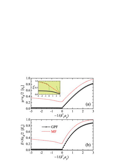
Figure 1: The chemical potential $\mu$ (in units of $\varepsilon_{F}$) and the total energy $E$ (in units of $E_{0}=N\varepsilon_{F}/2$), as a function of the inverse scattering area $-1/(k_{F}^{2}a_{p})$, calculated by using the mean-field theory (red dashed line) and the GPF theory (black solid line with circles). We have subtracted the contribution from the two-body bound state with binding energy $\varepsilon_{B}\equiv-E_{b}$ when the scattering area is positive. The effective range of the interaction is fixed to $k_{F}R_{p}=0.05$. The inset in (a) shows the pairing order parameter. The two green dot-dashed lines are the mean-field predictions of the asymptotic behavior in the BCS and BEC limits, Eqs. (29) and (31), respectively.

In the BEC limit, the chemical potential becomes negative and approaches the half of the bound state energy, i.e., $\mu\rightarrow-\hbar^{2}\kappa^{2}/(2M)$, where $\kappa$ is the solution of Eq. (13). From Eq. (27), it is readily seen that,

$$\frac{\Delta}{\varepsilon_{F}}\simeq\left[-\frac{1}{2}\ln\left(R_{p}\kappa\right)-\frac{1}{4}\right]^{-1/2}.$$ (31)

For the chemical potential, we rewrite it into the form, $\mu=-\hbar^{2}\kappa^{2}/(2M)+\mu_{B}/2$, where the molecular chemical potential $\mu_{B}$ is approximately equal to $g_{B}n_{2D}/2$ with $g_{B}$ being the strength of the interaction between two pairs. After some algebra, we find that

$$\frac{\mu_{B}}{\varepsilon_{F}}\simeq\left[-\frac{1}{2}\ln\left(R_{p}\kappa\right)-\frac{1}{4}\right]^{-1}\simeq\left(\frac{\Delta}{\varepsilon_{F}}\right)^{2}.$$ (32)

The pair-pair interaction strength $g_{B}=\mu_{B}/(n_{2D}/2)$ is then given by,

$$g_{B}\simeq\frac{8\pi\hbar^{2}/M}{-\ln\left(R_{p}\kappa\right)}=\frac{16\pi\hbar^{2}/M}{\ln\left[\hbar^{2}k_{0}^{2}/(M\left|E_{b}\right|)\right]},$$ (33)

in agreement with the previous result (see Eq. (48) in Ref. Hu2018 ).

III.2 Numerical results on equation of state

At the level beyond mean-field, the GPF theory can only be solved numerically. In Fig. 2, we report the GPF chemical potential (a), total energy (b) and the pairing gap (i.e., the inset) as a function of the inverse scattering area $-1/(k_{F}^{2}a_{p})$ at a given effective range $k_{F}R_{p}=0.05$, using the black solid lines with circles. For comparison, we show also the corresponding mean-field results by the red dashed lines. These thermodynamic variables have been shown in the previous work as a function of the scattering energy $E_{b}$ Hu2018 .

Both chemical potential and total energy suppress significantly from their non-interacting values $\varepsilon_{F}$ and $E_{0}=N\varepsilon_{F}/2$, respectively. In particular, on the BEC side, we observe a flat molecular chemical potential and total energy, which are nearly independent on the scattering area $a_{p}$. As discussed in the previous work Hu2018 , this is an indication of the formation of an interacting Bose condensate of composite Copper pairs in two dimensions, with a constant pair-pair interaction strength $g_{B}\sim\hbar^{2}/M$.

III.3 Super-Efimov trimers

It is worth mentioning that, for 2D fermions with $p$-wave interaction, Nishida and co-workers recently discovered a series of three-particle bound states, namely super-Efimov states Nishida2013 . How would the many-body properties of the system (i.e., contact and breathing mode as addressed in this work) be affected by these super-Efimov trimers is an interesting research topic to explore Zhang2017SuperEfimov . Naïvely, due to the double exponential scaling of the super-Efimov trimers Nishida2013 , we anticipate that only one trimer with an emergent energy scale will appear under current experimental conditions. The neighboring trimer with smaller energy cannot exist due to its large spatial extent, while the one with larger energy is simply too deep to be experimentally observed. In this respect, the impact of super-Efimov states to the many-body physics could be less significant than that of conventional Efimov states.

IV Results and discussions

We are now ready to discuss the $p$-wave contacts and the related breathing mode frequency. There are two contact parameters, characterizing the short-distance and large-momentum behaviors of different correlation functions, such as momentum distribution and pair-pair correlation function Yoshida2015 ; Yu2015 . As shown by Yi-Cai Zhang and Shizhong Zhang Zhang2017 , these two contacts $C_{a}$ and $C_{R}$ satisfy the adiabatic relations,

$$\left(\frac{\partial E}{\partial a_{p}^{-1}}\right)_{S} = -\frac{\pi\hbar^{2}}{2M}C_{a},$$ (34)

$$\left(\frac{\partial E}{\partial\ln R_{p}}\right)_{S} = \frac{\hbar^{2}}{M}C_{R},$$ (35)

and therefore can be determined once the total energy is known at a given entropy $S$. At zero temperature, where the entropy is always zero, we simply take the two first-order derivatives.

IV.1 Tan’s $p$-wave contacts

For this purpose, we may write the zero-temperature total energy in a dimensionless form $\xi(x,y)$,

$$E=\frac{N\varepsilon_{F}}{2}\xi\left[x\equiv\frac{1}{k_{F}^{2}a_{p}},y\equiv\ln\left(k_{F}R_{p}\right)\right],$$ (36)

and the two $p$-wave contacts can similarly be rewritten in the dimensionless way,

$$\frac{C_{a}}{N} = -\frac{1}{2\pi}\xi_{x},$$ (37)

$$\frac{C_{R}}{Nk_{F}^{2}} = \frac{1}{4}\xi_{y},$$ (38)

where $\xi_{x}\equiv\partial\xi/\partial x$ and $\xi_{y}\equiv\partial\xi/\partial y$. Following the dimensionless form of the total energy, it is easy to find that the chemical potential $\mu=\partial E/\partial N$ and the pressure $P=\mu n_{2D}-E/A$,

$$\mu = \varepsilon_{F}\left(\xi-\frac{x}{2}\xi_{x}+\frac{1}{4}\xi_{y}\right),$$ (39)

$$P = P_{0}\left(\xi-x\xi_{x}+\frac{1}{2}\xi_{y}\right),$$ (40)

where $P_{0}\equiv n_{2D}\varepsilon_{F}/2$. By substituting the expressions of the dimensionless contact into the last equation for pressure, we obtain the pressure relation Zhang2017 ,

$$PA=E+\frac{\pi\hbar^{2}}{2M}\frac{C_{a}}{a_{p}}+\frac{\hbar^{2}}{2M}C_{R}.$$ (41)

It is useful to distinguish the two- and many-body contributions to the contact parameters. For the two-body contribution, we assume that the system can be viewed as an ideal, non-interacting gas of $N/2$ pairs, each of which has the energy,

$$\varepsilon_{2B}=\left\{\begin{array}[]{cc}-\varepsilon_{B},&\textrm{if $a_{p}>0$}\\ 0,&\textrm{otherwise}\end{array}\right..$$ (42)

In other words, on the BEC side the pair takes the ground-state energy of the two-body bound state; while on the BCS side, the minimum energy of the pair should be zero (i.e., the lower threshold of the two-particle continuum). The two-body contribution to the total energy of the system can then be written as,

$$E_{2B}=\left(N/2\right)\varepsilon_{2B}=\left\{\begin{array}[]{cc}-N\varepsilon_{B}/2,&\textrm{if $a_{p}>0$}\\ 0,&\textrm{otherwise}\end{array}\right..$$ (43)

On the BEC side, by using Eq. (13), we find that the two-body contribution to the contact from the energy $E_{2B}$, denoted by $C_{a,2B}$ and $C_{R,2B}$, is given by Zhang2017 ,

$$C_{a,2B} = -\frac{N}{2}\frac{1}{\ln\left(R_{p}\kappa\right)+1/2},$$ (44)

$$C_{R,2B} = +\frac{N}{2}\frac{\kappa^{2}}{\ln\left(R_{p}\kappa\right)+1/2}.$$ (45)

On the BCS side, $C_{a,2B}=0$ and $C_{R,2B}=0$, as a result of $E_{2B}=0$. On both sides, either BEC or BCS, we obtain that,

$$E_{2B}+\frac{\pi\hbar^{2}}{2M}\frac{C_{a,2B}}{a_{p}}+\frac{\hbar^{2}}{2M}C_{R,2B}=0.$$ (46)

This equation is easy to understand from the pressure relation, since the two-body bound state does not contribute to the many-body observables such as pressure.

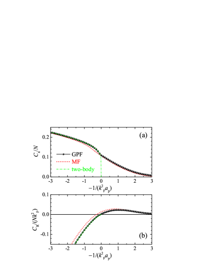
Figure 2: (color online). The contact parameters $C_{a}$ (a) and $C_{R}$ (b) as a function of the inverse scattering area $-1/(k_{F}^{2}a_{p})$ at the effective range of the interaction $k_{F}R_{p}=0.05$. The mean-field and GPF results are shown by the red dashed line and the black solid line with circles, respectively. The two-body contribution is also shown by the green dot-dashed line.

In Fig. 2, we plot the two dimensionless contact parameters as a function of $-1/(k_{F}^{2}a_{p})$ at a given effective range $k_{F}R_{p}=0.05$, calculated by using the GPF theory (black lines with circles) and the mean-field theory (red dashed lines). The two-body contribution from the bound state to the contacts is also shown by green dot-dashed lines. As we see in Fig. 2(a), the contact related to the scattering area $C_{a}$ is always positive. It increases with increasing interaction strength $(k_{F}^{2}a_{p})^{-1}$. On the BEC side with a positive scattering area, we find that the GPF result of $C_{a}$ is exhausted by the two-body contribution $C_{a,2B}$. The mean-field theory seems to under-estimate $C_{a}$, with the largest under-estimation occurs at $(k_{F}^{2}a_{p})^{-1}\sim 0.5$. On the other hand, the contact related to the effective range, $C_{R}$, has a non-monotonic dependence on the inverse scattering area, as shown in Fig. 2(b). As $(k_{F}^{2}a_{p})^{-1}$ increases, $C_{R}$ initially increases, reaches a maximum at $(k_{F}^{2}a_{p})^{-1}\sim-1$, and then decreases to zero at about the resonance limit. Towards the BEC limit, it decreases very rapidly. We find similarly that the GPF result of $C_{R}$ is almost exhausted by the two-body contribution $C_{R,2B}$. The mean-field theory generally over-estimates $C_{R}$ and the over-estimation becomes increasingly larger when we increase interaction strength. This is related to the unreliable prediction of the mean-field theory on the pair-pair interaction strength (see Eq. (33)).

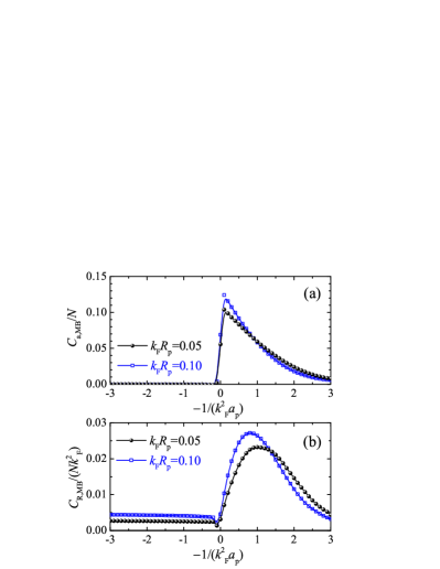
Figure 3: (color online). The many-body part of the contact parameters, $C_{a,MB}$ (a) and $C_{R,MB}$ (b), as a function of the inverse scattering area $-1/(k_{F}^{2}a_{p})$ at two effective ranges of the interaction $k_{F}R_{p}=0.05$ (black solid line with circles) and $k_{F}R_{p}=0.10$ (blue solid line with squares). All the results are calculated by using the GPF theory.

We have separated out the many-body parts of the two contact parameters, $C_{a,MB}=C_{a}-C_{a,2B}$ and $C_{R,MB}=C_{R}-C_{R,2B}$, and show the GPF predictions in Fig. 3, for two effective ranges of interactions, $k_{F}R_{p}=0.05$ (black line with circles) and $k_{F}R_{p}=0.10$ (blue line with squares). On the BEC side, the many-body parts of both contact parameters are small, consistent with the observation in Fig. 2 that the contacts are exhausted by the two-body contribution. Across the resonance limit, they exhibit a pronounced peak. The peak in $C_{a,MB}$ is slightly above the resonance limit. The peak in $C_{R,MB}$ locates at $(k_{F}^{2}a_{p})^{-1}\sim-1$ and shifts towards the BCS limit with decreasing effective range. We note that the many-body parts of the two $p$-wave contacts are always positive.

IV.2 Breathing mode frequency

The interesting dependence of the many-body part of the contacts on the interaction strength may lead to a non-trivial breathing-type oscillation mode, when the 2D $p$-wave Fermi superfluid is confined in a harmonic trap with trapping frequency $\omega_{0}$. This is a mode excited by the perturbation $\lambda(t)\mathcal{O}\equiv\lambda(t)\sum_{i=1}^{N}r_{i}^{2}$, i.e., by slightly modulating the harmonic trapping frequency for a certain period. For non-interacting bosons or fermions, the breathing mode frequency is simply $\omega_{c}=2\omega_{0}$. The inter-particle interaction generally leads to a frequency shift. As shown by Yi-Cai Zhang and Shizhong Zhang Zhang2017 , the frequency shift at the leading order is proportional to the contact parameters. By using virial expansion, the frequency shift of the breathing mode at high temperatures was then theoretically studied Zhang2017 .

In our zero-temperature case, we calculate the breathing mode frequency using the well-known scaling approach Menotti2002 ; Hu2004 ; Hu2014 . This amounts to assuming a polytropic form for the pressure equation of state, $P\propto n_{2D}^{\gamma+1}$, where the polytropic index $\gamma$ may be calculated using

$$\gamma=\frac{n_{2D}}{P}\left(\frac{\partial P}{\partial n_{2D}}\right)-1,$$ (47)

at the center of the harmonic trap. The scaling approach then leads to a breathing mode frequency Hu2014 ,

$$\frac{\omega_{B}^{2}}{\omega_{c}^{2}}=\frac{\gamma+1}{2}=\frac{P_{0}\kappa_{T}^{(0)}}{P\kappa_{T}},$$ (48)

where at zero temperature we rewrite $\partial P/\partial n_{2D}$ in terms of the compressibility $\kappa_{T}=[n_{2D}^{2}(\partial\mu/\partial n_{2D})]^{-1}$ and $\kappa_{T}^{(0)}\equiv(n_{2D}\varepsilon_{F})^{-1}$ is its non-interacting value. This expression emphasizes the sound-wave nature of the breathing mode frequency. Qualitatively, the breathing mode frequency can be estimated as $c_{s}k_{\textrm{min}}$, where $c_{s}$ is the sound velocity and $k_{\textrm{min}}\propto A^{-1/2}$ is the minimum wavevector of the Fermi cloud with an area $A$. By recalling the relation $\kappa_{T}^{-1}\propto c_{s}^{2}$ and assuming the pressure $P\propto A^{-1}$ under the soft-wall confinement of the harmonic trap, we find $\omega_{B}^{2}\propto(P\kappa_{T})^{-1}$.

The polytropic index $\gamma$ can be directly calculated once the energy or pressure equation of state is known. By taking derivative with respect to density in Eq. (40) and neglecting all small second-order derivatives, we find that,

$$n_{2D}\frac{\partial P}{\partial n_{2D}}\simeq 2P+P_{0}\left(-x\bar{\xi}_{x}+\frac{1}{2}\bar{\xi}_{y}\right),$$ (49)

where the bar over $\xi_{x}$ and $\xi_{y}$ indicates that we do not include the irrelevant two-body contribution. By substituting it into Eq. (47), we obtain the frequency shift $\delta\omega_{B}=\omega_{B}-\omega_{c}$,

$$\frac{\delta\omega_{B}}{\omega_{c}}\simeq\frac{\gamma-1}{4}\simeq\frac{-x\bar{\xi}_{x}+\frac{1}{2}\bar{\xi}_{y}}{4P/P_{0}}.$$ (50)

By replacing the two derivatives with the help of Eqs. (37) and (38), we finally arrive at

$$\frac{\delta\omega_{B}}{\omega_{c}}\simeq\frac{\hbar^{2}}{M^{2}}\frac{\left[\pi a_{p}^{-1}C_{a,MB}+C_{R,MB}\right]}{4\omega_{0}^{2}\left\langle\mathcal{O}\right\rangle},$$ (51)

where the virial theorem $PA=M\omega_{0}^{2}\left\langle\mathcal{O}\right\rangle/2$ in the presence of harmonic traps is used NoteVirialTheorem . We therefore recover Eq. (84) in Ref. Zhang2017 and explicitly show the relation between the many-body parts of the two $p$-wave contacts and the frequency shift in the breathing mode.

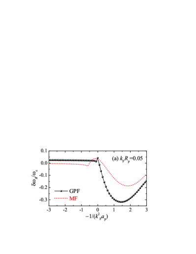
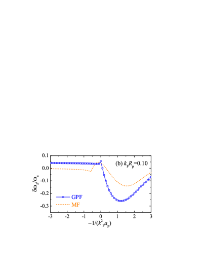
Figure 4: (color online). The deviation of the breathing mode frequency from the scale-invariant result of $\omega_{c}=2\omega_{0}$, as a function of the inverse scattering area $-1/(k_{F}^{2}a_{p})$, at two effective ranges of the interaction: $k_{F}R_{p}=0.05$ (a) and $k_{F}R_{p}=0.10$ (b). The mean-field and GPF results are shown by the dashed lines and the solid lines with symbols, respectively.

In Fig. 4, we present the frequency shift of the breathing mode as a function of the inverse scattering area, at two effective ranges $k_{F}R_{p}=0.05$ (a) and $k_{F}R_{p}=0.10$ (b). These results are calculated using Eq. (48) within the mean-field theory (dashed lines) and the GPF theory (lines with symbols). We find that the frequency shift is negative on the BCS side and exhibits a broad dip at $-(k_{F}^{2}a_{p})^{-1}\sim 1-2$. This dip structure is apparently related to the peak structure in the many-body part of the two $p$-wave contacts, according to Eq. (51). The two contacts contribute differently in opposite signs and the contribution from $C_{a,MB}$ seems to dominate. We note that, in a 1D harmonically trapped $p$-wave Fermi superfluid, the breathing mode frequency shows qualitatively similar dependence on the interacting strength in the weak-coupling regime Imambekov2010 ; Chen2016 .

On the BEC side, we see that the frequency shift predicted by the GPF theory becomes flat and small. This is associated with the formation of tight-binding molecules who interact via a nearly constant molecular scattering length, as we discussed earlier. The GPF frequency shift is positive and is about 5% at $k_{F}R_{p}=0.10$. In contrast, the mean-field frequency shift is negative and shows a non-trivial cusp at $(k_{F}^{2}a_{p})^{-1}\sim 0.5$. This mean-field behavior is unphysical, arising from the unreliable equations of state predicted by the mean-field theory. It is interesting to note that, the breathing mode frequency shift of a weakly-interacting 2D Bose gas was investigated both theoretically and experimentally Olshanii2010 ; Merloti2013 . In that case, the shift is too small to be experimentally observed. The moderately interacting molecular condensate formed in the strongly-interacting 2D $p$-wave Fermi superfluid could be a possible candidate to observe the breathing mode frequency shift due to beyond-mean-field effects.

V Frequency shift in the resonance limit

Here we focus on the breathing mode frequency in the resonance limit $a_{p}=\pm\infty$. If we neglect the dependence of the equations of state on the effective range, the dimensionless energy function $\xi$ is simply a constant. From the pressure $P=\xi P_{0}\propto n_{2D}^{2}$, we find a polytropic index $\gamma=2$ and hence $\omega_{B}=2\omega_{0}$. This could be an exact result ensured by the scale invariance of the system Werner2006 . However, the necessary existence of the effective range breaks the scale invariance and leads to a derivation of the breathing mode frequency away from the scale-invariant result of $\omega_{c}=2\omega_{0}$. A similar situation happens in an $s$-wave 2D Fermi superfluid Hofmann2012 ; Vogt2012 . While the superfluid with $s$-wave contact interaction is scale invariant in the classical treatment, i.e., the model Hamiltonian simply scales upon stretching the length of the system Pitaevskii1997 , the renormalization of the contact interaction necessarily introduces a 2D $s$-wave scattering length $a_{2D}$ that violates the scale-invariance. This leads to an up-shift in the breathing mode frequency, the so-called quantum anomaly, which is about 10% in the strongly-interacting regime Hofmann2012 ; Taylor2012 . It is not a surprise to see the similarity between the effective range $R_{p}$ in a $p$-wave Fermi superfluid and the 2D scattering length $a_{2D}$ in an $s$-wave Fermi superfluid. This is discussed in more detail in Appendix B.

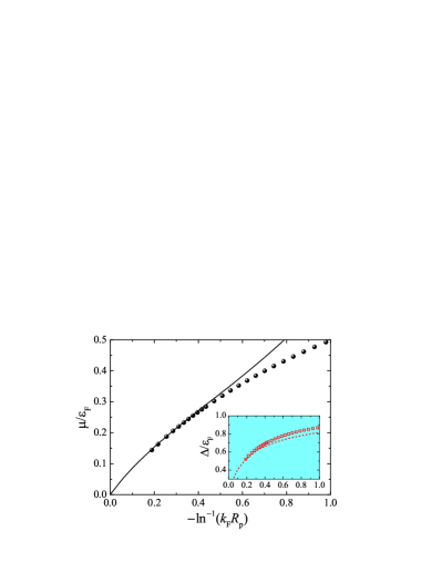
Figure 5: (color online). The mean-field chemical potential $\mu$ (main figure, circles) and the mean-field pairing order parameter (inset, squares) as a function of $-\ln^{-1}(k_{F}R_{p})$ in the resonance limit (i.e., $a_{p}\rightarrow\pm\infty$). The lines show the asymptotic behavior in the limit of zero effective range of the interaction, $R_{p}\rightarrow 0$ or $-\ln^{-1}(k_{F}R_{p})\rightarrow 0$, see, Eqs. (54) and (55).

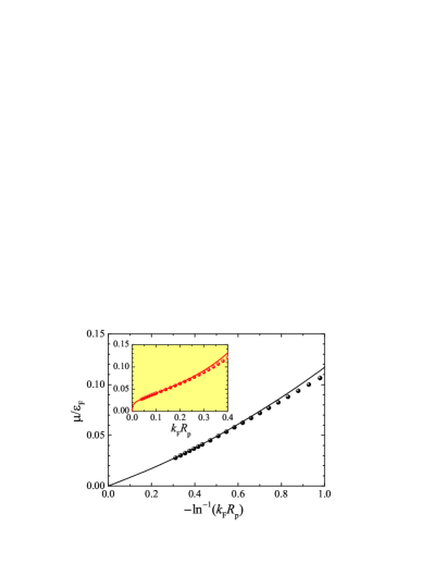
Figure 6: (color online). The chemical potential $\mu$ as a function of $-\ln^{-1}(k_{F}R_{p})$, calculated by using the GPF theory in the resonance limit $a_{p}\rightarrow\pm\infty$. The inset shows the chemical potential as a function of $k_{F}R_{p}$ in the linear scale. The lines are the fitting curves to the GPF results, see Eq. (56).

V.1 Chemical potential in the resonance limit

Before we discuss the frequency shift in a resonantly interacting $p$-wave Fermi superfluid, it is useful to first understand the chemical potential in this limit. Using the mean-field equations Eqs. (19) and (20), we find that,

$$\tilde{\mu} = -\frac{1}{\ln\left(k_{F}R_{p}\tilde{\Delta}/2\right)},$$ (52)

$$\tilde{\Delta}^{2} = \frac{2\tilde{\mu}\left(1-\tilde{\mu}\right)}{1-\tilde{\mu}/2}.$$ (53)

By treating $-[\ln(k_{F}R_{p})]^{-1}=-y^{-1}$ as the small parameter, we obtain,

$$\frac{\mu}{\varepsilon_{F}} \simeq -\frac{1}{y}\left[1-\frac{1}{2y}\ln\left(-\frac{1}{2y}\right)\right],$$ (54)

$$\frac{\Delta}{\varepsilon_{F}} \simeq \sqrt{-\frac{2}{y}}\left[1-\frac{1}{4y}\ln\left(-\frac{1}{2e}\frac{1}{y}\right)\right].$$ (55)

Thus, towards the zero-range limit, the mean-field chemical potential at resonance vanishes linearly.

More accurate predictions from the GPF theory should be determined numerically. Empirically, we find that the GPF chemical potential at resonance can be nicely fitted by the formalism,

$$\frac{\mu}{\varepsilon_{F}}\simeq-A\left(\frac{1}{y}-\frac{1}{2y^{2}}\right),$$ (56)

where $A\simeq 0.078\ll 1$. While the GPF chemical potential at resonance still vanishes linearly in the zero-range limit, the slope (i.e., the value of $A$) is much slower than that of the mean-field chemical potential.

In Figs. (5) and (6), we report the mean-field and GPF predictions of the chemical potential at resonance as a function of $-\ln^{-1}(k_{F}R_{p})$, respectively. The analytic expressions and the empirical formalism discussed in the above are also shown. At small effective range, they agree well with the numerical results.

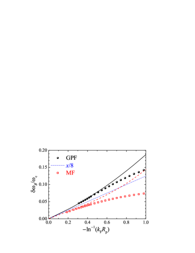
Figure 7: (color online). The deviation of the breathing mode frequency from the scale-invariant result of $\omega_{c}=2\omega_{0}$ as a function of $-\ln^{-1}(k_{F}R_{p})$ in the resonance limit $a_{p}\rightarrow\pm\infty$. The mean-field and GPF results are shown by the black circles and red squares, respectively. The black solid line and red dashed line are the corresponding analytical results in the zero-range limit, Eq. (60) and Eq. (59). The blue dot-dashed line shows the leading contribution to the deviation of the mode frequency: $\delta\omega_{B}/(2\omega_{0})\simeq-\ln^{-1}(k_{F}R_{p})/8$; see, Eq. (58).

V.2 Frequency shift

The mean-field analytic expression and the GPF empirical formalism for the chemical potential at resonance are very useful to understand the shift of the breathing mode frequency. To see this, we may calculate the polytropic index related to the chemical potential, i.e., $\mu\propto n_{2D}^{\gamma}$, by using

$$\gamma=\frac{n_{2D}}{\mu}\left(\frac{\partial\mu}{\partial n_{2D}}\right)\simeq 1+\frac{\xi_{y}^{(\mu)}}{2\xi^{(\mu)}},$$ (57)

where we have rewritten $\mu=\varepsilon_{F}\xi^{(\mu)}(y)$ and have assumed $\xi_{y}^{(\mu)}\ll\xi^{(\mu)}$. By taking the chemical potential at the leading order, i.e., $\xi^{(\mu)}\propto-1/y$, we obtain immediately $\gamma\simeq 1-1/[2\ln(k_{F}R_{p})]$, and consequently,

$$\frac{\delta\omega_{B}}{\omega_{c}}\simeq\frac{\gamma-1}{4}\simeq-\frac{1}{8y}=-\frac{1}{8\ln\left(k_{F}R_{p}\right)}.$$ (58)

More careful treatments of the chemical potential to the next order in Eqs. (54) and Eq. (56) lead to the results,

$$\frac{\delta\omega_{B}}{\omega_{c}}\simeq-\frac{1}{8y}\left[1-\frac{1}{2y}\ln\left(-\frac{e}{2y}\right)\right]$$ (59)

for the mean-field theory and

$$\frac{\delta\omega_{B}}{\omega_{c}}\simeq-\frac{1}{8y}\left[1-\frac{1}{2y}\right]$$ (60)

for the GPF theory, respectively.

In Fig. 7, we show the up-shifts of the breathing mode frequency predicted by the mean-field theory and the GPF theory in the resonance limit, together with the asymptotic behaviors in the zero-range limit, as discussed in the above. According to the GPF theory, the shift of the breathing mode frequency can easily reach 10% at a relatively small effective range, i.e., $[\ln(k_{F}R_{p})]^{-1}\simeq-0.6$ or $k_{F}R_{p}\sim 0.2$.

At this point, it is interesting to compare the frequency shift exhibited by a resonantly interacting $p$-wave Fermi superfluid and by a strongly interacting $s$-wave Fermi superfluid, both in two dimensions. In the latter case, the theoretically predicted maximum quantum anomaly of 10% is yet to be experimentally confirmed Vogt2012 ; Holten2018 ; Peppler2018 . The main obstacle comes from the confinement-induced effective range $R_{s}$, which is significant under the current experimental condition. Indeed, our recent analysis indicates that the effective range $R_{s}$ in a 2D $s$-wave superfluid can strongly suppress the quantum anomaly down to 1-2% Hu2019 . In sharp contrast, for a resonantly interacting $p$-wave Fermi superfluid, the effective range $R_{p}$ enhances the frequency shift. Owing to the great feasibility in tuning $R_{p}$ in cold-atom experiment, therefore, we anticipate that a low-temperature $p$-wave Fermi gas at Feshbach resonances would be an ideal candidate to conclusively confirm the predicted frequency shift.

VI Conclusions and outlooks

In conclusions, we have theoretically determined two important experimental observables - Tan’s contact parameter and the breathing mode frequency - of a resonantly interacting $p$-wave Fermi superfluid in two dimensions at the BEC-BCS evolution. Both observables can be easily accessed in current cold-atom experiment, as soon as a stable $p$-wave superfluid is realized in reduced dimensions. The two Tan’s contact parameters can be directly extracted from the tail of momentum distribution probed by radio-frequency spectroscopy Luciuk2016 , and the breathing mode measurement is now a routine tool in cold-atom laboratories Vogt2012 ; Holten2018 ; Peppler2018 .

We have proposed that, similar to an $s$-wave Fermi superfluid at the BEC-BCS crossover, the $p$-wave Fermi superfluid in the resonance limit experiences a frequency shift, due to the non-vanishing effective range of interactions that explicitly breaks the scale invariance of the system. The up-shift in the breathing mode frequency, away from the scale-invariant value $\omega_{c}=2\omega_{0}$, turns out to be significant. At the leading order, it is inversely proportional to the logarithm of the effective range. As a result of this slow-decay logarithmic dependence, the frequency shift can reach 5-10% over a wide range of the effective range.

Appendix A An integral in the two-body $T$-matrix

Here we consider the integral,

$$\mathcal{I} =\mathcal{\mathscr{P}}\sum_{{\bf p}}\frac{\left|\Gamma\left({\bf p}\right)\right|^{2}}{2\epsilon_{{\bf p}}-E},$$

$$=\frac{M}{\hbar^{2}k_{F}^{2}}\intop_{0}^{\infty}\frac{pdp}{2\pi}\frac{p^{2}}{\left[1+\left(p/k_{0}\right)^{2n}\right]^{3}}\mathcal{\mathscr{P}}\frac{1}{p^{2}-k^{2}}.$$ (61)

By introducing the variable $z\equiv(p/k_{0})^{2}$, we find that,

$$\mathcal{I}=\frac{Mk_{0}^{2}}{4\pi\hbar^{2}k_{F}^{2}}\intop_{0}^{\infty}dz\frac{z}{\left(1+z^{n}\right)^{3}}\mathcal{\mathscr{P}}\frac{1}{z-z_{0}},$$ (62)

where $z_{0}\equiv(k/k_{0})^{2}\ll 1$. To handle the operator $\mathcal{\mathscr{P}}$ for Cauchy principle value, we divide the whole integral into three parts $[0,z_{0})\cup[z_{0},2z_{0})\cup[2z_{0},\infty)$. Upon changing the dummy variable, the integral $\mathcal{I}$ can be rewritten in terms of $I_{1}$ and $I_{2}$,

$$\mathcal{I}=\frac{Mk_{0}^{2}}{4\pi\hbar^{2}k_{F}^{2}}\left[I_{1}+I_{2}\right],$$ (63)

where

$$I_{1}=\intop_{0}^{z_{0}}\frac{dz}{z}\left\{\frac{z_{0}+z}{\left[1+\left(z_{0}+z\right)^{n}\right]^{3}}-\frac{z_{0}-z}{\left[1+\left(z_{0}-z\right)^{n}\right]^{3}}\right\}$$ (64)

and

$$I_{2}=\intop_{z_{0}}^{\infty}\frac{dz}{z}\frac{z_{0}+z}{\left[1+\left(z_{0}+z\right)^{n}\right]^{3}}.$$ (65)

It is clear that $I_{1}=2z_{0}+o(z_{0})$. For $I_{2}$, by neglecting the higher contribution $o(z_{0})$, it can be separated into two parts,

$$I_{2}=-2z_{0}+\intop_{0}^{\infty}\frac{dz}{\left(1+z^{n}\right)^{3}}+z_{0}\intop_{z_{0}}^{\infty}\frac{dz}{z\left(1+z^{n}\right)^{3}}.$$ (66)

These two parts can be integrated out explicitly:

$$\intop_{0}^{\infty}\frac{dz}{\left(1+z^{n}\right)^{3}} = \frac{\pi\left(n-1/2\right)\left(n-1\right)}{n^{3}\sin\left(\pi/n\right)},$$ (67)

$$\intop_{z_{0}}^{\infty}\frac{dz}{z\left(1+z^{n}\right)^{3}} = -\ln z_{0}-\frac{3}{2n}+\frac{3z_{0}^{n}}{n}+o(z_{0}^{n}).$$ (68)

Putting $I_{1}$ and $I_{2}$ together, up to the order $o(z_{0})$ we obtain the expression,

$$\mathcal{I}=\frac{Mk_{0}^{2}}{4\pi\hbar^{2}k_{F}^{2}}\left[\frac{\pi\left(n-\frac{1}{2}\right)\left(n-1\right)}{n^{3}\sin\left(\pi/n\right)}-z_{0}\ln z_{0}-\frac{3z_{0}}{2n}\right].$$ (69)

which is Eq. (9) in the main text.

Appendix B Quantum anomaly in a strongly interacting $s$-wave Fermi superfluid

In an $s$-wave Fermi superfluid, Tan’s adiabatic relation is given by Werner2012 ,

$$\left(\frac{\partial E}{\partial\ln a_{2D}}\right)_{S}=\frac{\hbar^{2}}{2\pi M}C,$$ (70)

which takes exactly the same form as the adiabatic relation for the effective range of interactions, as given in Eq. (35), up to an unimportant pre-factor. This same form emphasizes the similar role played by the effective range $R_{p}$ in a $p$-wave Fermi superfluid and by the scattering length $a_{2D}$ in an $s$-wave Fermi superfluid.

Let us now write the total energy of the $s$-wave Fermi superfluid in a dimensionless form He2015 ,

$$E=\frac{N\varepsilon_{F}}{2}\xi\left[z=\ln\left(k_{F}a_{2D}\right)\right],$$ (71)

where for the two-component Fermi gas the Fermi wavevector $k_{F}=\sqrt{2\pi n_{2D}}.$ By using the adiabatic relation Eq. (70), we then find,

$$\frac{C}{k_{F}^{4}}=\frac{1}{4}\xi_{z},$$ (72)

where $\xi_{z}=\partial\xi/\partial z$. The dimensionless chemical potential and pressure are also easy to obtain,

$$\mu = \varepsilon_{F}\left(\xi+\frac{1}{4}\xi_{z}\right),$$ (73)

$$P = P_{0}\left(\xi+\frac{1}{2}\xi_{z}\right).$$ (74)

By calculating the polytropic index related to the pressure Hofmann2012 , we find that,

$$\gamma=\frac{n_{2D}}{P}\left(\frac{\partial P}{\partial n_{2D}}\right)-1\simeq 1+\frac{\bar{\xi}_{z}}{2\bar{\xi}},$$ (75)

where again the bar denotes the exclusion of the two-body bound-state contribution. The calculation of the polytropic index related to the chemical potential leads to the same expression at the same level of approximation. Thus, we obtain the quantum anomaly,

$$\frac{\delta\omega_{B}}{2\omega_{0}}\simeq\frac{\gamma-1}{4}\simeq\frac{\bar{\xi}_{z}}{8\bar{\xi}}=\frac{C_{MB}/k_{F}^{4}}{2(E+N\varepsilon_{B}/2)/E_{0}}.$$ (76)

According to the GPF calculation or quantum Monte Carlo simulations, at around the strongly interacting regime $\ln\left(k_{F}a_{2D}\right)\sim 0$, the many-body part of the contact shows a peak with $C_{MB}/k_{F}^{4}\sim 0.05$ He2015 . This is correlated with a total energy $(E+N\varepsilon_{B}/2)/E_{0}\sim 0.25$ He2015 . By using these two numbers, we find a quantum anomaly $\delta\omega_{B}/(2\omega_{0})\sim 0.1$ for a strongly interacting $s$-wave Fermi superfluid.

References

- (1) C. Chin, R. Grimm, P. Julienne, and E. Tiesinga, Rev. Mod. Phys. 82, 1225 (2010).
- (2) D. M. Eagles, Phys. Rev. 186, 456 (1969).
- (3) A. J. Leggett, in Modern Trends in the Theory of Condensed Matter, edited by A. Pekalski and R. Przystaw (Springer-Verlag, Berlin, 1980).
- (4) P. Noziéres and S. Schmitt-Rink, J. Low Temp. Phys. 59, 195 (1985).
- (5) C. A. R. Sá de Melo, M. Randeria, and J. R. Engelbrecht, Phys. Rev. Lett. 71, 3202 (1993).
- (6) C. A. Regal, M. Greiner, and D. S. Jin, Phys. Rev. Lett. 92, 040403 (2004).
- (7) M. W. Zwierlein, C. A. Stan, C. H. Schunck, S. M. F. Raupach, A. J. Kerman, and W. Ketterle, Phys. Rev. Lett. 92, 120403 (2004).
- (8) H. Hu, X.-J. Liu, and P. D. Drummond, Europhys. Lett. 74, 574 (2006).
- (9) R. B. Diener, R. Sensarma, and M. Randeria, Phys. Rev. A 77, 023626 (2008).
- (10) I. Bloch, J. Dalibard, and W. Zwerger, Rev. Mod. Phys. 80, 885 (2008).
- (11) S. Giorgini, L. P. Pitaevskii, and S. Stringari, Rev. Mod. Phys. 80, 1215 (2008).
- (12) C. A. Regal, C. Ticknor, J. L. Bohn, and D. S. Jin, Phys. Rev. Lett. 90, 053201 (2003).
- (13) J. Zhang, E. G. M. van Kempen, T. Bourdel, L. Khaykovich, J. Cubizolles, F. Chevy, M. Teichmann, L. Tarruell, S. J. J. M. F. Kokkelmans, and C. Salomon, Phys. Rev. A 70, 030702(R) (2004).
- (14) K. Günter, T. Stöferle, H. Moritz, M. Köhl, and T. Esslinger, Phys. Rev. Lett. 95, 230401 (2005).
- (15) C. H. Schunck, M. W. Zwierlein, C. A. Stan, S. M. F. Raupach, W. Ketterle, A. Simoni, E. Tiesinga, C. J. Williams, and P. S. Julienne, Phys. Rev. A 71, 045601 (2005).
- (16) J. P. Gaebler, J. T. Stewart, J. L. Bohn, and D. S. Jin, Phys. Rev. Lett. 98, 200403 (2007).
- (17) J. Fuchs, C. Ticknor, P. Dyke, G. Veeravalli, E. Kuhnle, W. Rowlands, P. Hannaford, and C. J. Vale, Phys. Rev. A 77, 053616 (2008).
- (18) Y. Inada, M. Horikoshi, S. Nakajima, M. Kuwata-Gonokami, M. Ueda, and T. Mukaiyama, Phys. Rev. Lett. 101, 100401 (2008).
- (19) N. Read and D. Green, Phys. Rev. B 61, 10267 (2000).
- (20) D. A. Ivanov, Phys. Rev. Lett. 86, 268 (2001).
- (21) A. Yu. Kitaev, Ann. Phys. (NY) 303, 2 (2003).
- (22) For a review, see, C. Nayak, S. H. Simon, A. Stern, M. Freedman, and S. D. Sarma, Rev. Mod. Phys. 80, 1083 (2008).
- (23) For a review, see V. Gurarie and L. Radzihovsky, Ann. Phys. (Amsterdam) 322, 2 (2007).
- (24) S. S. Botelho and C. A. R. Sa de Melo, J. Low Temp. Phys. 140, 409 (2005).
- (25) T.-L. Ho and R. B. Diener, Phys. Rev. Lett. 94, 090402 (2005).
- (26) V. Gurarie, L. Radzihovsky, and A. V. Andreev, Phys. Rev. Lett. 94, 230403 (2005).
- (27) C.-H. Cheng and S.-K. Yip, Phys. Rev. Lett. 95, 070404 (2005).
- (28) M. Iskin and C. A. R. Sá de Melo, Phys. Rev. Lett. 96, 040402 (2006).
- (29) G. Cao, L. He, and P. Zhuang, Phys. Rev. A 87, 013613 (2013).
- (30) Y. Ohashi, Phys. Rev. Lett. 94, 050403 (2005).
- (31) D. Inotani, R. Watanabe, M. Sigrist, and Y. Ohashi, Phys. Rev. A 85, 053628 (2012).
- (32) D. Inotani and Y. Ohashi, Phys. Rev. A 92, 063638 (2015).
- (33) G. Cao, L. He, and X.-G. Huang, Phys. Rev. A 96, 063618 (2017).
- (34) C. Luciuk, S. Trotzky, S. Smale, Z. Yu, S. Zhang, and J. H. Thywissen, Nat. Phys. 12, 599 (2016).
- (35) M. Waseem, T. Saito, J. Yoshida, and T. Mukaiyama, Phys. Rev. A 96, 062704 (2017).
- (36) J. Yoshida, T. Saito, M. Waseem, K. Hattori, and T. Mukaiyama, Phys. Rev. Lett. 120, 133401 (2018).
- (37) M. Waseem, J. Yoshida, T. Saito, and T. Mukaiyama, Phys. Rev. A 98, 020702(R) (2018).
- (38) S. Tan, Ann. Phys. (NY) 323, 2952 (2008).
- (39) S. Tan, Ann. Phys. (NY) 323, 2971 (2008).
- (40) S. Tan, Ann. Phys. (NY) 323, 2987 (2008).
- (41) S. M. Yoshida and M. Ueda, Phys. Rev. Lett. 115, 135303 (2015).
- (42) Z. Yu, J. H. Thywissen, and S. Zhang, Phys. Rev. Lett. 115, 135304 (2015).
- (43) M. He, S. Zhang, H. M. Chan, and Q. Zhou, Phys. Rev. Lett. 116, 045301 (2016).
- (44) S.-G. Peng, X.-J. Liu, and H. Hu, Phys. Rev. A 94, 063651 (2016).
- (45) Y.-C. Zhang and S. Zhang, Phys. Rev. A 95, 023603 (2017).
- (46) J. Yao and S. Zhang, Phys. Rev. A 97, 043612 (2018).
- (47) D. Inotani and Y. Ohashi, Phys. Rev. A 98, 023603 (2018).
- (48) J. Levinsen, N. R. Cooper, and V. Gurarie, Phys. Rev. A, 78, 063616 (2008).
- (49) A. K. Fedorov, V. I. Yudson, and G. V. Shlyapnikov, Phys. Rev. A 95, 043615 (2017).
- (50) H. Hu, B. C. Mulkerin, L. He, J. Wang, and X.-J. Liu, Phys. Rev. A 98, 063605 (2018).
- (51) H. Hu, P. D. Drummond, and X.-J. Liu, Nat. Phys. 3, 469 (2007).
- (52) L. He, H. Lü, G. Cao, H. Hu, and X.-J. Liu, Phys. Rev. A 92, 023620 (2015).
- (53) Z. Yu, G. M. Bruun, and G. Baym, Phys. Rev. A 80, 023615 (2009).
- (54) X.-J. Liu, H. Hu, and P. D. Drummond, Phys. Rev. Lett. 102, 160401 (2009).
- (55) H. Hu, X.-J. Liu, and P. D. Drummond, New J. Phys. 13, 035007 (2011).
- (56) X.-J. Liu, Phys. Rep. 524, 37 (2013).
- (57) F. Werner and Y. Castin, Phys. Rev. A 74, 053604 (2006).
- (58) L. P. Pitaevskii and A. Rosch, Phys. Rev. A 55, R853 (1997).
- (59) J. Hofmann, Phys. Rev. Lett. 108, 185303 (2012).
- (60) E. Taylor and M. Randeria, Phys. Rev. Lett. 109, 135301 (2012).
- (61) C. Gao and Z. Yu, Phys. Rev. A 86, 043609 (2012).
- (62) E. Vogt, M. Feld, B. Fröhlich, D. Pertot, M. Koschorreck, and M. Köhl, Phys. Rev. Lett. 108, 070404 (2012).
- (63) B. C. Mulkerin, X.-J. Liu, and H. Hu, Phys. Rev. A 97, 053612 (2018).
- (64) M. Holten, L. Bayha, A. C. Klein, P. A. Murthy, P. M. Preiss, and S. Jochim, Phys. Rev. Lett. 121, 120401 (2018).
- (65) T. Peppler, P. Dyke, M. Zamorano, S. Hoinka, and C. J. Vale, Phys. Rev. Lett. 121, 120402 (2018).
- (66) H. Hu, B. C. Mulkerin, U. Toniolo, L. He, and X.-J. Liu, Phys. Rev. Lett. 122, 070401 (2019).
- (67) A. A. Abrikosov, L. Gor’kov, and I. E. Dzyaloshinski, Methods of Quantum Field Theory in Statistical Physics (Dover, New York, 1963).
- (68) Y. Nishida, S. Moroz, and D. T. Son, Phys. Rev. Lett. 110, 235301 (2013).
- (69) P. Zhang and Z. Yu, Phys. Rev. A 95, 033611 (2017).
- (70) C. Menotti and S. Stringari, Phys. Rev. A 66, 043610 (2002).
- (71) H. Hu, A. Minguzzi, X.-J. Liu, and M. P. Tosi, Phys. Rev. Lett. 93, 190403 (2004).
- (72) H. Hu, P. Dyke, C. J. Vale, and X.-J. Liu, New J. Phys. 16, 083023 (2014).
- (73) There is a subtlety here, as we want to relate the peak value of a quantity at the trap center to an average of the quantity over the whole trap. In a 2D harmonic trap, the virial theorem states that the trapping potential energy . In the last step, we approximate the integral using the peak pressure at the trap center and define an appropriate area , which is to be removed by using the identity .
- (74) A. Imambekov, A. A. Lukyanov, L. I. Glazman, and V. Gritsev, Phys. Rev. Lett. 104, 040402 (2010).
- (75) X.-L. Chen, X.-J. Liu, and H. Hu, Phys. Rev. A 94, 033630 (2016).
- (76) M. Olshanii, H. Perrin, and V. Lorent, Phys. Rev. Lett. 105, 095302 (2010).
- (77) K. Merloti, R. Dubessy, L. Longchambon, M. Olshanii, and H. Perrin, Phys. Rev. A 88, 061603 (2013).
- (78) F. Werner and Y. Castin, Phys. Rev. A 86, 013626 (2012).