Region-Manipulated Fusion Networks for Pancreatitis Recognition

Abstract

This work first attempts to automatically recognize pancreatitis on CT scan images. However, different form the traditional object recognition, such pancreatitis recognition is challenging due to the fine-grained and non-rigid appearance variability of the local diseased regions. To this end, we propose a customized Region-Manipulated Fusion Networks (RMFN) to capture the key characteristics of local lesion for pancreatitis recognition. Specifically, to effectively highlight the imperceptible lesion regions, a novel region-manipulated scheme in RMFN is proposed to force the lesion regions while weaken the non-lesion regions by ceaselessly aggregating the multi-scale local information onto feature maps. The proposed scheme can be flexibly equipped into the existing neural networks, such as AlexNet and VGG. To evaluate the performance of the propose method, a real CT image database about pancreatitis is collected from hospitals . And experimental results on such database well demonstrate the effectiveness of the proposed method for pancreatitis recognition.

ancreatitis Recognition, Deep Learning, Medical Image, Fusion Networks.

1 Introduction

The physiological and pathological changes of the pancreas are closely related to life. Acute Pancreatitis (AP) is one of the most common gastrointestinal disorder requiring inpatient admission all over the world [1]. A large part of the patients (15$\sim$20%) develop severe AP, which is characterized by persistent organ failure, resulting in significant morbidity and mortality [2, 3, 4]. Severe AP has a higher mortality rate, which has attracted widespread attention in the last ten years. Therefore, it is urgent to diagnose this dangerous diseases accurately in the critical early phase of the AP.

As we know, Computed Tomography (CT) is a widely-used technology that provides a common way for the diagnose of AP in the early phase. Generally, a radiologist makes a primary diagnosis, the clinician can then make a definite diagnosis via the radiologist’s decision, laboratory data and clinical manifestation. However, there are some shortcomings in such diagnose approaches. Firstly, radiologists are difficult to keep absolute objectivity due to limitations of their own knowledge and experience. Secondly, reading CT is a time-consuming and labor consuming work. Finally, the size of early lesions is usually small and the characteristics are generally not obvious enough, which easily leads to missed diagnosis.

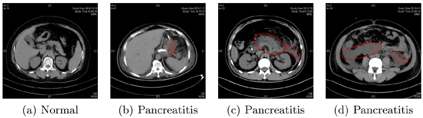
Figure 1: Comparisons of different abdominal CT scan images. The lesion regions are outlined in red circles. It is obvious that the lesion area has only a small local area in the whole image and most area of the image is normal. (a) normal abdominal CT scan image. (b) fluid collection in omental bursa and posterior gastric space. (c) pancreatic swelling and fluid collection in the left anterior pararenal space. (d) fluid collection in paracolic space.

Recently, inspired by the tremendous development of computer vision and machine learning, intelligent medical diagnosis [5] explores to automatically recognize whether there are certain diseases on CT scan images. This can not only greatly improve the efficiency of diagnosis, but also avoid the human subjectivity and even misdiagnosis as much as possible. At present, deep learning has outperformed traditional machine learning algorithms in various vision problems, e.g., natural image classification [6], object detection [5], and face recognition [7], etc. The excellent performance of deep learning in computer vision has attracted the attention of medical image processing researchers. However, most existing deep learning models are designed for natural images, which consider the whole image instead of the local area. In contrast, medical images have large intra-class variation and inter-class ambiguity. In addition, in the medical image of a patient, lesion area providing valuable information is usually small, while most areas are normal. Undoubtedly, faced with this challenging task, several early-bird researchers have designed various architectures of deep networks for some specific tasks, such as diabetic retinopathy detection [8], skin cancer classification [9], and lung nodule classification [10], etc.

Inspired by the above work, we first attempts to automatically recognize pancreatitis on abdominal CT scan images by leveraging the superior power of deep learning. However, according to the investigation with the collaboration of doctors in the early stage, image recognition of pancreatitis has to face with several specific challenges compared with existing deep learning based medical analysis methods. As shown in Figure 1, three great challenges are summarized as follows, (1) fine-grained recognition. The lesion area only providing the valuable information is very small. (2) intra-class variation and inter-class ambiguity. The intra-class variation between images from the same class is common, and the inter-class difference between images from different classes is ambiguous. (3) Non-rigid object. The lesion region doesn’t have a certain shape and size.

After above analysis, we propose a customized Region-Manipulated Fusion Networks (RMFN) to automatically recognize pancreatitis on the abdominal CT scan images in this work. First, to solve this fine-grained recognition, we adopt a deep network architecture to learn the high-level representations of the CT images. Second, to avoid intra-class variation and inter-class ambiguity, we also capture the local discriminative information from the local view by taking the small regions as the input of the subnetworks. Finally, to highlight the non-rigid lesion, a novel region-manipulated scheme is proposed to force the lesion regions while weaken the non-lesion regions by ceaselessly aggregating the multi-scale local information onto feature maps. Specifically, we fuse multi-scale feature maps from the FCN of main-network and sub-networks, and then the fused feature map is input to the next FCN of main-network. To well evaluate the performance of the proposed method, we collect a real-world CT image database about pancreatitis from hospitals, and conduct experiments on such database to well demonstrate the effectiveness of the proposed method.

In summary, the main contributions of this work are two-fold: (1) To the best of our knowledge, our work is the first time to leverage a novel CNN architecture to solve the problem of pancreatitis recognition, and contribute a database of abdominal CT scan images on the community of medical image analysis. (2) We propose a novel region-manipulated scheme to enhance small yet discriminative information regions of images. The proposed scheme can be flexibly equipped into the existing neural networks to improve the performance of image classification and object recognition in the community of computer vision.

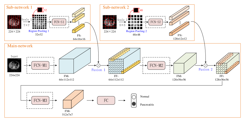
Figure 2: The architecture of the proposed networks. The architecture has three networks consists of a main-network and two sub-networks. The input image consists of three scales. The feature map $FS_{1}$ of sub-network 1 and feature map $FM_{1}$ from FCN-M1 of main-network are fused to $FF_{1}$ in fusion 1 strategy. The feature map $FS_{2}$ of sub-network 2 and feature map $FM_{2}$ from FCN-M2 of main-network are fused to $FF_{2}$ in fusion 2 strategy. FCN-M3 of main-network takes $FF_{2}$ as input and outputs $FM_{3}$. Finally, the FC of main-network takes $FM_{3}$ as input and outputs predicted results.

2 Related works

In this section, we give a brief review to deep learning and medical image analysis with deep learning.

2.1 Deep learning in computer vision

As a feature learning method, deep learning [11] can transform raw data into a higher level and more abstract representation. These abstract representations are advantageous to learn essential features of images [12]. Therefore, deep learning has brought a breakthrough in many fields of computer vision, such as face recognition [13, 14], image classification [15, 16, 17], object detection [5, 18], image segmentation [19, 20, 21], etc.

Many variants of deep learning models have been proposed for the last five years, such as AlexNet [6], VGG [22], GoogleNet [17], ResNet [23], and so on. In the image classification field, Krizhevsky et al. proposed AlexNet and achieved great improvement compared with the other methods on the ILSVRC-2012 classification task [6]. He et al. proposed a Deep Residual Learning model and achieved encouraging results on the ILSVRC-2015 classification task [23]. In the object detection field, Girshick proposed a Fast R-CNN to speed up the detection and improve detection accuracy on the image detection filed [5]. In the image segmentation field, Chen et al. presented a Deeplab for semantic image segmentation and achieved the-state-of-art results at the PASCAL VOC-2012 semantic image segmentation task [19].

The excellent performance of CNN in computer vision attracted great attention of medical image researchers. More and more medical image researchers are applying CNN to solve the tasks of medical images, such as classification [9, 24, 25], detection [26, 27], segmentation  [28, 29, 30], etc.

2.2 Medical image analysis with deep learning

There are a large number of medical image data in medical institutions, such as CT scan images. These medical images usually contain a great deal of potential information [31]. Therefore, we need to make full use of these large amounts of data and potential information. The diagnosis usually relies on doctors’ expert knowledge that may be time consuming and information loss. Recently, the rapid development of deep learning provides a feasible solution for the development of medical automation.

Some medical image researchers began to study many specific diseases. For example, Esteva et al. used deep learning methods to classify skin cancer diseases, and the diagnostic accuracy was comparable to that of human doctors [9]. Gulshan et al. employed the deep learning methods to detect the diabetic retinopathy  [8]. Gao et al. applied deep learning methods to classify interstitial lung diseases imaging patterns on CT images [32]. However, the performance of deep learning lies on the larger scale database. In fact, there is only a few of high-quality annotated database of medical images available. Usually, once a large-scale medical image database is reported, there will be emerging several works to solve various problems on this database. For example, lung nodules on CT scans is collected by Armato et al. [33], subsequently, there emerged a lot of studies on recognizing lung nodules with deep learning methods [10, 34, 35].

In the field of medical analysis, many researchers focus on the network structures to make them more suitable for specific diseases. Gao et al. proposed a novel framework that combines CNN and RNN for cataract grading and achieved the state-of-the-art performance [36]. Kamnitsas et al. proposed a dual pathway architecture to process the input images at multiple scales [37]. They make full use of multi-scale contextual information and thus achieve a satisfactory performance. Inspired by above works, we also attempt to re-design the deep learning architecture to recognize pancreatitis on abdominal CT scan images in this work.

3 The proposed method

In order to recognize pancreatitis accurately, we propose a customized Region-Manipulated Fusion Networks (RMFN) by ceaselessly aggregating the multi-scale local information onto feature maps. Here, the proposed region-manipulated scheme can be incorporated into the existing neural networks, such as AlexNet [6] and VGG [22]. In this section, we take VGG11 as the base networks to describe the proposed RMFN.

3.1 Network architecture

The architecture of the proposed RMFN is shown in Figure 2. It can be seen that RMFN consists of a main-network and two sub-networks. Main-network aims to capture the global information, while sub-networks are used to force obtain local discriminative information. Fusion of main-network and sub-networks can enhance the ability of model to highlight the local lesion of abdominal CT images with pancreatitis. Given an image, a fully convolutional network M1 (FCN-M1) takes it as input and outputs the corresponding feature map $FM_{1}(a)$. To obtain multi-scale information, we use two other scales (i.e., $G_{1}\times G_{1}$ and $G_{2}\times G_{2}$ grids, respectively).

At scale 1 ($\alpha 1$ for short), we divide the input image into $G_{1}\times G_{1}$ regions $\{R_{\alpha 1}^{m,n}\}_{m,n}^{G_{1}}$ by a Region Pooling 1 strategy and put them into a Fully Convolutional Network S1 (FCN-S1) to output the corresponding feature maps $FS_{1}(R_{\alpha 1}^{m,n}$). Here, $R_{\alpha 1}^{m,n}$ denotes the $m$-row and $n$-column region, $m,n=1,2,...,G_{1}$.

Once the feature maps $FS_{1}(R_{\alpha 1}^{m,n})$ and $FM_{1}(a)$ are obtained, we take a fusion mechanism (i.e., fusion 1) to fuse these two features and generate a new feature maps $FF_{1}(a)$. The $G_{1}\times G_{1}$ local regions of feature maps $FM_{1}(a)$ can be represented as follows:

$$M_{\alpha 1}^{m,n}:\left\{\begin{aligned} (m-1)L_{\alpha 1}/2\leq{i}\leq{mL_{\alpha 1}/2}\\ (n-1)L_{\alpha 1}/2\leq{j}\leq{nL_{\alpha 1}/2}\end{aligned}\right.$$ (1)

where, $M_{\alpha 1}^{m,n}$ is the $m$-row, $n$-column grid region of $FM_{1}(a)$, $L_{\alpha 1}$ is the size of a grid region $R_{\alpha 1}^{m,n}$. $i,j\in\mathbb{N}^{*}$.

After getting the feature map $FF_{1}(a)$, the Fully Convolutional Network M2 (FCN-M2) takes it as input and the feature map $FM_{2}(a)$ is obtained. Similar to the scale 1, at scale 2 ($\alpha 2$ for short), we divide the input image into $G_{2}\times G_{2}$ equal regions $R_{\alpha 2}^{m,n}$ by the Region Pooling 2 strategy and put them into a Fully Convolutional Network S2 (FCN-S2) to output the corresponding feature maps $FS_{2}(R_{\alpha 2}^{m,n})$, where $m,n=1,2,...,G_{2}$.

Once the feature maps $FS_{2}(R_{\alpha 2}^{m,n})$ and $FM_{2}(a)$ are obtained, we take a fusion mechanism (fusion 2) to fuse the two features and generate new feature maps $FF_{2}(a)$. The $G_{2}\times G_{2}$ corresponding regions of feature maps $FM_{2}(a)$ are represented as follows:

$$M_{\alpha 2}^{m,n}:\left\{\begin{aligned} (m-1)(L_{\alpha 2}-\epsilon)/4\leq{i}\leq{m(L_{\alpha 2}-\epsilon)/4+\epsilon/4}\\ (n-1)(L_{\alpha 2}-\epsilon)/4\leq{j}\leq{n(L_{\alpha 2}-\epsilon)/4+\epsilon/4}\end{aligned}\right.$$ (2)

where, $M_{\alpha 2}^{m,n}$ is the $m$ row, $n$ column grid region of $FM_{2}(a)$. $L_{\alpha 2}$ is the side length of the square grid region $R_{\alpha 2}^{m,n}$. $i,j\in\mathbb{N}^{*}$.

After getting feature map $FF_{2}(a)$, a Fully Convolutional Network M3 (FCN-M3) takes it as input and the feature map $FM_{3}(a)$ is obtained. Finally, the Fully Connected networks (FC) takes feature maps $FM_{3}(a)$ as input and outputs two-dimensional vector $(x,y)$. More specially, if $x>y$, it indicates that the person is normal in terms to the pancreas, otherwise pancreatitis patient.

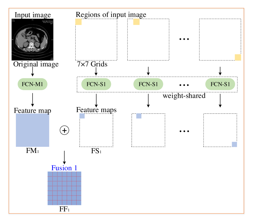
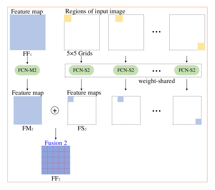
Figure 3: Two types of Fusion strategies on feature maps. (a) shows that the feature map $FM_{1}$ of original image obtained by FCN-M1 and the feature map $FS_{1}$ of Scale 1 (e.g. $7\times 7$ grids) image obtained by FCN-S1 are added to feature map $FF_{1}$. (b) shows that the feature map $FM_{2}$ of $FF_{1}$ obtained by FCN-M2 and the feature map $FS_{2}$ of Scale 2 (e.g. $5\times 5$ grids) image obtained by FCN-S2 are added to feature map $FF_{2}$.

3.2 Region pooling

The texture feature of local region contains important discriminant information. The focus of the paper is to capture texture of non-rigid region. We can strengthen the ability of capture with specific multi-scale grid.

In order to divide the grid reasonably and obtain multi-scale information, we take a region pooling mechanism to divide the input image into multiple equal regions. The proposed fusion method of this work including two types of strategies: Region Pooling 1 and Region Pooling 2. The strategy of Region Pooling 1 is formulated as:

$$R_{\alpha 1}^{m,n}:\left\{\begin{aligned} (m-1)L_{\alpha 1}\leq{i}\leq{mL_{\alpha 1}}\\ (n-1)L_{\alpha 1}\leq{j}\leq{nL_{\alpha 1}}\end{aligned}\right.$$ (3)

where $R_{\alpha 1}^{m,n}$ ($m,n=1,2,...,G_{1}$) is the $m$ row, $n$ column grid region of input image, $L_{\alpha 1}$ is the size of the square grid region $R_{\alpha 1}^{m,n}$, and $i,j\in\mathbb{N}^{*}$.

Unlike the Region Pooling 1 strategy, the Region Pooling 2 strategy is only used to solve the existence of the overlap area between two adjacent grid regions. Specifically, the method of Region Pooling 2 is formulated as:

$$R_{\alpha 2}^{m,n}:\left\{\begin{aligned} (m-1)(L_{\alpha 2}-\epsilon)\leq{i}\leq{m(L_{\alpha 2}-\epsilon)+\epsilon}\\ (n-1)(L_{\alpha 2}-\epsilon)\leq{j}\leq{n(L_{\alpha 2}-\epsilon)+\epsilon}\end{aligned}\right.$$ (4)

where $i,j\in\mathbb{N}^{*}$, $R_{\alpha 2}^{m,n},m,n=1,2,...,G_{2}$ is the $m$ row, $n$ column grid region of input image, $L_{\alpha 2}$ is size of a square grid region $R_{\alpha 2}^{m,n}$, and $\epsilon$ is the width of the overlap area between arbitrary two adjacent grid regions. It is noted that $L_{\alpha 2}$ and $\epsilon$ satisfy the following formula:

$$(G_{2}-1)\epsilon-G_{2}L_{\alpha 2}+L_{0}=0$$ (5)

where $L_{0}\times L_{0}$ is the size of the input image.

3.3 Fusion strategy

In order to make full use of multi-scale feature maps, we take a fusion mechanism to fuse the two features from main-network and sub-network respectively and generate new feature maps. In this work, according to the two types of region pooling strategies, the designed fusion strategy includes two type of versions: Fusion 1 and Fusion 2. First, the Fusion 1 strategy can be formulated as:

$$D_{\alpha 1}^{m,n}=\sum\limits_{j=1}^{L_{\alpha 1}/2}\sum\limits_{i=1}^{L_{\alpha 1}/2}u_{i,j}^{m,n}+U_{P_{\alpha 1}(i,m),Q_{\alpha 1}(j,n)}^{m,n}$$ (6)

where $P_{\alpha 1}(i,m)=i+(m-1)L_{\alpha 1}/2$, $Q_{\alpha 1}(j,n)=j+(n-1)L_{\alpha 1}/2$, $u_{i,j}^{m,n}$ is the $i$ row, $j$ column value of the $m$ row, $n$ column region $FS_{1}(R_{\alpha 1}^{m,n})$. $U_{P_{\alpha 1}(i,m),Q_{\alpha 1}(j,n)}^{m,n}$ is the $i$ row, $j$ column value of the region $M_{\alpha 1}^{m,n}$. $D_{\alpha 1}^{m,n}$ is the whole values of the $m$ row, $n$ column regions $M_{\alpha 1}^{m,n}$. Figure 3(a) shows the detailed steps of the Fusion 2 strategy.

Unlike Fusion 1, Fusion 2 is only used to solve the existence of the overlap area between two adjacent grid regions. Fusion 2 can be formulated as:

$$D_{\alpha 2}^{m,n}=\sum\limits_{j=1}^{L_{\alpha 2}/4}\sum\limits_{i=1}^{L_{\alpha 2}/4}v_{i,j}^{m,n}+V_{P_{\alpha 2}(i,m),Q_{\alpha 2}(j,n)}^{m,n}$$ (7)

where $P_{\alpha 2}(i,m)=i+(m-1)(L_{\alpha 2}-\epsilon)/4$, $Q_{\alpha 2}(j,n)=j+(n-1)(L_{\alpha 2}-\epsilon)/4$. $v_{i,j}^{m,n}$ is the $i$-row, $j$-column value of the $m$-row, $n$-column region $FS_{2}(R_{\alpha 2}^{m,n})$. $V_{P_{\alpha 2}(i,m),Q_{\alpha 2}(j,n)}^{m,n}$ is the $i$-row, $j$ column-value of the corresponding region $M_{\alpha 2}^{m,n}$. $D_{\alpha 2}^{m,n}$ is the value after fusing the $m$ row and $n$ column regions $M_{\alpha 2}^{m,n}$. Figure 3(b) shows the detailed steps of the Fusion 2 strategy.

3.4 Implementation details

In this paper, we take a VGG11 as the base networks to introduce the implementation details of the proposed RMFN. The architecture and configuration of the proposed RMFN is shown in Figure 2 and Table 1, respectively. We can see that the parameter of feature maps $FM_{1}(a)$ is $64\times 112\times 112$, where 64 denotes the number of feature maps, and $112\times 112$ denotes the size of one feature map. Based on the validation for different scales, the parameter $G_{1}$ of Scale 1 and the parameter $G_{2}$ of Scale 2 are set to 7 and 5, respectively. Correspondingly, the parameter $L_{\alpha 1}$ of Region Pooling 1 and the parameter $L_{\alpha 2}$ of Region Pooling 2 are set to 32 and 48, respectively. In particular, at scale 2, the width $\epsilon$ of the overlap area between two adjacent grid regions is set to 4.

Table 1: Model configurations of the networks. For example, conv3 and 64 of conv3-64 denote $3\times 3$ convolution kernel and the number of feature map, respectively. 4096 of FC-4096 denotes the parameter number of the fully connected layer.

Original configuration		Configuration of the proposed network architecture
FCN	FC	FCN-M1	FCN-M2	FCN-M3	FCN-S1	FCN-S2	FC
conv3-64	FC-4096	conv3-64	conv3-128	conv3-256	conv3-64	conv3-64	FC-4096
maxpool	FC-4096	maxpool	maxpool	conv3-256	maxpool	maxpool	FC-4096
conv3-128	FC-2			maxpool		conv3-128	FC-2
maxpool				conv3-512		maxpool
conv3-256				conv3-512
conv3-256				maxpool
maxpool				conv3-512
conv3-512				conv3-512
conv3-512				maxpool
maxpool
conv3-512
conv3-512
maxpool

In this work, the size of the input abdominal CT image is set to a $224\times 224$. Due to the difference of convolution schemes, the sizes of multi-scale image of different networks are also different. Specifically, when main-network is VGG11 or VGG16, the resolution of multi-scale images is $224\times 224$, $48\times 48$ ($5\times 5$ grids) and $32\times 32$ ($7\times 7$ grids); when main-network is AlexNet, the resolution of multi-scale images is $224\times 224$, $48\times 48$ ($5\times 5$ grids) and $36\times 36$ ($7\times 7$ grids). Since the number of VGG16 network parameter is relatively large, which requires much GPU memory, we reduce the number of VGG16 network parameters on a degree, namely the number of parameters is reduced to half. We implement the proposed RMFN on PyTorch platform, and choose the stochastic gradient descent (SGD) to update the parameters of the model. The dropout rate, the momentum, batch size and learning rate are set to 0.5 and 0.9, 64 and 0.001, respectively.

4 Experiments

To evaluate the performance of the proposed method, we collect a real CT image database about pancreatitis from hospitals and conduct experiments on this database. Besides, we also visualize the feature maps of the proposed RMFN and the baseline network models to illustrate the superiority of the proposed region-manipulated scheme.

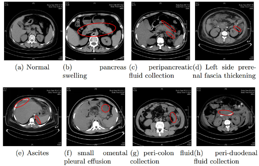
Figure 4: Comparisons of different abdominal CT scan images.(a) normal abdominal CT scan image. (b) pancreas swelling. (c) peripancreatic fluid collection. (d) left side prerenal fascia thickening. (e) ascites. (f)small omental pleural effusion. (g) peri-colon fluid collection. (h) peri-duodenal fluid collection.

4.1 Database collection

Since there is no public dataset used to evaluate the performance for the pancreatitis recognition task, we collect abdominal CT scan images with the size of $512\times 512$ from hospital and build a database of Abdominal CT Images about Pancreatitis (ACIP). ACIP consists of 2500 normal abdominal CT images and 2500 abdominal CT images of pancreatitis patients. Three doctors with years of clinical experience are invited to annotate the images. Each image is annotated with 0 or 1, where 0 denotes a normal abdominal CT image and 1 denotes an abdominal CT image of pancreatitis patients. To learn and test models, this ACIP database is divided into two parts: 80% for training and 20% for testing.

Table 2: The number of images on the ACIP database. There are 4000 training images and 1000 testing images.

Database	normal	pancreatitis
$\sharp$ training images	2000	2000
$\sharp$ testing images	500	500
$\sharp$ total	2500	2500

To better annotate CT images, we first analyze the abdominal CT scan images from pancreatitis patients and healthy people, and observe that the pancreatitis is determined by the small lesion area rather than most of areas as shown in Figure 4. For most of the abdominal CT images of pancreatitis patients, the lesion area mainly has the following characteristics: pancreas swelling, peripancreatic fluid collection, left side prerenal fascia thickening, ascites, small omental pleural effusion, peri-colon fluid collection, and peri-duodenal fluid collection. Our doctors give the results of diagnosis based on the above characteristics.

4.2 Experimental settings

To show the effectiveness of the proposed method for pancreatitis recognition, we compare it with the shallow method (i.e., SVM [38]), and the classic deep learning models (i.e., AlexNet [6], VGG11 [22] and VGG16 [22]). For SVM, we reduce the size of the input image from $512\times 512$ to $224\times 224$ and extract features by SVD.

In experiments, the following three baselines are also implemented to illustrate the effectiveness of the proposed region-manipulated scheme in RMFN: (1)Original CNN (i.e., VGG11, VGG16, and AlexNet). The original CNN directly extracts features from the whole image and obtains the global information. This baseline can illustrate the importance of deep features. (2)M-RMNF-A (M is VGG11, VGG16, or AlexNet). This baseline extracts features from the whole image and small local areas at Scale 1. (3)M-RMNF-B (M is VGG11, VGG16, or AlexNet). This baseline extracts features from the whole image and big local areas at Scale 2. Accordingly, for such three types of deep networks, the proposed RMFN also has three versions, termed as M-RMFN-C (i.e., VGG11-RMFN-C, VGG16-RMNF-C, and AlexNet-RMFN-C). The evaluation criterions include the recognition accuracy, precision, recall and F1 score.

4.3 Results and analysis

Table 2 lists the results of 12 different networks on the collected ACIP database in terms of recognition accuracy, precision, recall and F1 on the ACIP database. We can see that AlexNet-RMFN-C achieves the best performance. For convenient comparison, we put the model with the same base networks into a family. For each family, the proposed M-RMFN-C achieves better performance than the other baselines. In particular, for the VGG16 family, VGG16-RMFN-C improves about 4.1% compared with the original VGG16. It is indicated M-RMFN-C capturing the multi-scale local information is superior to M-RMFN-A and M-RMFN-B targeting only single-scale local information.

Table 3: Performance comparison with different baseline networks on the ACIP database.

model	Scale	precision($\%$)	recall($\%$)	F1($\%$)	accuracy($\%$)
SVM	$224\times 224$	$79.6$	$78.6$	$79.1$	$78.6$
VGG11	$224\times 224$	$87.8$	$96.0$	$91.7$	$91.3$
VGG11-RMFN-A	$224\times 224+32\times 32$	$88.4$	$96.0$	$92.0$	$91.7$
VGG11-RMFN-B	$224\times 224+48\times 48$	$89.1$	$94.8$	$91.9$	$91.6$
VGG11-RMFN-C	$224\times 224+48\times 48+32\times 32$	$90.2$	$97.4$	$93.7$	$93.4$
VGG16	$224\times 224$	$87.9$	$94.2$	$90.9$	$90.6$
VGG16-RMFN-A	$224\times 224+32\times 32$	$91.4$	$97.8$	$94.5$	$94.3$
VGG16-RMFN-B	$224\times 224+48\times 48$	$90.3$	$97.2$	$93.6$	$93.4$
VGG16-RMFN-C	$224\times 224+48\times 48+32\times 32$	$92.1$	$97.8$	$94.9$	$94.7$
AlexNet	$224\times 224$	$92.8$	$98.6$	$95.6$	$95.5$
AlexNet-RMFN-A	$224\times 224+36\times 36$	$93.7$	$98.4$	$96.0$	$95.9$
AlexNet-RMFN-B	$224\times 224+48\times 48$	$94.1$	$98.8$	$96.4$	$96.3$
AlexNet-RMFN-C	$224\times 224+48\times 48+36\times 36$	$95.3$	$98.2$	$96.7$	$96.7$

To further illustrate our networks architecture better, we visualize the learned features to intuitively compare the proposed RMFN and baselines, as shown in Figure 5. We visualize feature maps of final convolutional layers and added the feature map to original image by suitable weights. Figure 5(a) shows input CT scan images of pancreatitis, where the areas of pancreatic fluid are outlined in red circles. Figure 5(b), Figure 5(c), Figure 5(d) and Figure 5(e) are the visualized features learned from AlexNet, AlexNet-RMFN-C, VGG16, and VGG16-RMFN-C, respectively. Comparing with the features of AlexNet and VGG16, the proposed AlexNet-RMFN-c and VGG16-RMFN-C locate the lesion areas more accurately.

5 Conclusion

In this work, we proposed a novel Region-Manipulated Fusion Networks (RMFN) architecture to recognize pancreatitis on the abdominal CT scan images by capturing the key characteristics of the local lesion. In particular, a novel region-manipulated scheme in RMFN can effectively highlight the imperceptible lesion regions by aggregating the multi-scale local information into feature maps. This region-manipulated scheme can enhance the local discriminative region, meanwhile, weaken the non-discriminative regions. To evaluate the performance of the propose method, we build a high-quality abdominal CT image database with/without pancreatitis. Finally, we conduct experiments to demonstrate the effectiveness of the proposed method for pancreatitis recognition. In future work, we will push the region-manipulated idea into the powerful Generative Adversarial Net and further improve the performance of pancreatitis recognition.

References

- [1] D. Yadav and A. B. Lowenfels, “The epidemiology of pancreatitis and pancreatic cancer,” Gastroenterology, vol. 144, no. 6, pp. 1252–1261, 2013.
- [2] P. A. Banks, T. L. Bollen, C. Dervenis, H. G. Gooszen, C. D. Johnson, M. G. Sarr, G. G. Tsiotos, and S. S. Vege, “Classification of acute pancreatitis—2012: revision of the atlanta classification and definitions by international consensus,” GUT, vol. 62, no. 1, pp. 102–111, 2013.
- [3] G. M. Cavestro, G. Leandro, M. Di L., R. A. Zuppardo, O. B. Morrow, C. Notaristefano, G. Rossi, S. G. G. Testoni, G. Mazzoleni, M. Alessandri et al., “A single-centre prospective, cohort study of the natural history of acute pancreatitis,” Digestive and Liver Disease, vol. 47, no. 3, pp. 205–210, 2015.
- [4] H. Nawaz, R. Mounzer, D. Yadav, J. G. Yabes, A. Slivka, D. C. Whitcomb, and G. I. Papachristou, “Revised atlanta and determinant-based classification: application in a prospective cohort of acute pancreatitis patients,” AJG, vol. 108, no. 12, p. 1911, 2013.
- [5] R. Girshick, “Fast r-cnn,” in ICCV, 2015.
- [6] A. Krizhevsky, I. Sutskever, and G. E. Hinton, “Imagenet classification with deep convolutional neural networks,” in NIPS, 2012.
- [7] Y. Sun, X. Wang, and X. Tang, “Deeply learned face representations are sparse, selective, and robust,” in CVPR, 2015, pp. 2892–2900.
- [8] V. Gulshan, L. Peng, M. Coram, M. C. Stumpe, D. Wu, A. Narayanaswamy, S. Venugopalan, K. Widner, T. Madams, J. Cuadros et al., “Development and validation of a deep learning algorithm for detection of diabetic retinopathy in retinal fundus photographs,” JAMA, vol. 316, no. 22, pp. 2402–2410, 2016.
- [9] A. Esteva, B. Kuprel, R. A. Novoa, J. Ko, S. M. Swetter, H. M. Blau, and S. Thrun, “Dermatologist-level classification of skin cancer with deep neural networks,” Nature, vol. 542, no. 7639, pp. 115–118, 2017.
- [10] R. Golan, C. Jacob, and J. Denzinger, “Lung nodule detection in ct images using deep convolutional neural networks,” in IJCNN, 2016.
- [11] Y. LeCun, Y. Bengio, and G. Hinton, “Deep learning,” Nature, vol. 521, no. 7553, pp. 436–444, 2015.
- [12] B. Zhou, A. Khosla, A. Lapedriza, A. Oliva, and A. Torralba, “Learning deep features for discriminative localization,” in CVPR. IEEE, 2016, pp. 2921–2929.
- [13] O. M. Parkhi, A. Vedaldi, A. Zisserman et al., “Deep face recognition.” in BMVC, 2015.
- [14] W. Liu, Y. Wen, Z. Yu, M. Li, B. Raj, and L. Song, “Sphereface: Deep hypersphere embedding for face recognition,” in CVPR, 2017, pp. 212–220.
- [15] Z. Akata, F. Perronnin, Z. Harchaoui, and C. Schmid, “Good practice in large-scale learning for image classification,” IEEE TPAMI, vol. 36, no. 3, pp. 507–520, 2014.
- [16] F. Wang, M. Jiang, C. Qian, S. Yang, C. Li, H. Zhang, X. Wang, and X. Tang, “Residual attention network for image classification,” in CVPR, 2017, pp. 3156–3164.
- [17] C. Szegedy, W. Liu, Y. Jia, P. Sermanet, S. Reed, D. Anguelov, D. Erhan, V. Vanhoucke, and A. Rabinovich, “Going deeper with convolutions,” in CVPR, 2015.
- [18] S. Ren, K. He, R. Girshick, and J. Sun, “Faster r-cnn: Towards real-time object detection with region proposal networks,” in NIPS, 2015.
- [19] L.-C. Chen, G. Papandreou, I. Kokkinos, K. Murphy, and A. L. Yuille, “Deeplab: Semantic image segmentation with deep convolutional nets, atrous convolution, and fully connected crfs,” IEEE TPAMI, vol. 40, no. 4, pp. 834–848, 2017.
- [20] V. Badrinarayanan, A. Kendall, and R. Cipolla, “Segnet: A deep convolutional encoder-decoder architecture for image segmentation,” IEEE TPAMI, vol. 39, no. 12, pp. 2481–2495, 2017.
- [21] L.-C. Chen, Y. Zhu, G. Papandreou, F. Schroff, and H. Adam, “Encoder-decoder with atrous separable convolution for semantic image segmentation,” in ECCV, 2018, pp. 801–818.
- [22] K. Simonyan and A. Zisserman, “Very deep convolutional networks for large-scale image recognition,” arXiv, 2014.
- [23] K. He, X. Zhang, S. Ren, and J. Sun, “Deep residual learning for image recognition,” in CVPR, 2016.
- [24] J. Ren, I. Hacihaliloglu, E. A. Singer, D. J. Foran, and X. Qi, “Adversarial domain adaptation for classification of prostate histopathology whole-slide images,” in MICCAI. Springer, 2018, pp. 201–209.
- [25] J. Zhang, Y. Xie, Q. Wu, and Y. Xia, “Skin lesion classification in dermoscopy images using synergic deep learning,” in MICCAI. Springer, 2018, pp. 12–20.
- [26] F. Liao, M. Liang, Z. Li, X. Hu, and S. Song, “Evaluate the malignancy of pulmonary nodules using the 3-d deep leaky noisy-or network,” IEEE TNNLS, 2019.
- [27] W. Zhu, C. Liu, W. Fan, and X. Xie, “Deeplung: Deep 3d dual path nets for automated pulmonary nodule detection and classification,” in WACV. IEEE, 2018, pp. 673–681.
- [28] A. Farag, L. Lu, H. R. Roth, J. Liu, E. Turkbey, and R. M. Summers, “A bottom-up approach for pancreas segmentation using cascaded superpixels and (deep) image patch labeling,” IEEE TIP, vol. 26, no. 1, pp. 386–399, 2017.
- [29] Y. Man, Y. Huang, J. F. X. Li, and F. Wu, “Deep q learning driven ct pancreas segmentation with geometry-aware u-net,” IEEE TMI, 2019.
- [30] Q. Yu, L. Xie, Y. Wang, Y. Zhou, E. K. Fishman, and A. L. Yuille, “Recurrent saliency transformation network: Incorporating multi-stage visual cues for small organ segmentation,” in CVPR, 2018, pp. 8280–8289.
- [31] P. Lambin, E. Rios-Velazquez, R. Leijenaar, S. Carvalho, R. G. van Stiphout, P. Granton, C. M. Zegers, R. Gillies, R. Boellard, A. Dekker et al., “Radiomics: extracting more information from medical images using advanced feature analysis,” EJC, vol. 48, no. 4, pp. 441–446, 2012.
- [32] M. Gao, U. Bagci, L. Lu, A. Wu, M. Buty, H. C. Shin, H. Roth, G. Z. Papadakis, A. Depeursinge, R. M. Summers et al., “Holistic classification of ct attenuation patterns for interstitial lung diseases via deep convolutional neural networks,” CMBBE: Imaging & Visualization, pp. 1–6, 2016.
- [33] S. G. Armato, G. McLennan, L. Bidaut, M. F. McNitt-Gray, C. R. Meyer, A. P. Reeves, B. Zhao, D. R. Aberle, C. I. Henschke, E. A. Hoffman et al., “The lung image database consortium (lidc) and image database resource initiative (idri): a completed reference database of lung nodules on ct scans,” Medical Physics, vol. 38, no. 2, pp. 915–931, 2011.
- [34] A. A. A. Setio, F. Ciompi, G. Litjens, P. Gerke, C. Jacobs, S. J. van R., M. M. W. Wille, M. Naqibullah, C. I. Sánchez, and B. van G., “Pulmonary nodule detection in ct images: false positive reduction using multi-view convolutional networks,” IEEE TMI, vol. 35, no. 5, pp. 1160–1169, 2016.
- [35] H. C. Shin, H. R. Roth, M. Gao, L. Lu, Z. Xu, I. Nogues, J. Yao, D. Mollura, and R. M. Summers, “Deep convolutional neural networks for computer-aided detection: Cnn architectures, dataset characteristics and transfer learning,” IEEE TMI, vol. 35, no. 5, pp. 1285–1298, 2016.
- [36] X. Gao, S. Lin, and T. Y. Wong, “Automatic feature learning to grade nuclear cataracts based on deep learning,” IEEE TBE, vol. 62, no. 11, pp. 2693–2701, 2015.
- [37] K. Kamnitsas, C. Ledig, V. F. Newcombe, J. P. Simpson, A. D. Kane, D. K. Menon, D. Rueckert, and B. Glocker, “Efficient multi-scale 3d cnn with fully connected crf for accurate brain lesion segmentation,” Medical image analysis, vol. 36, pp. 61–78, 2017.
- [38] J. A. Suykens and J. Vandewalle, “Least squares support vector machine classifiers,” NPL, vol. 9, no. 3, pp. 293–300, 1999.