OGLE-2018-BLG-1011Lb,c: Microlensing Planetary System with Two Giant Planets Orbiting a Low-mass Star

Abstract

We report a multiplanetary system found from the analysis of microlensing event OGLE-2018-BLG-1011, for which the light curve exhibits a double-bump anomaly around the peak. We find that the anomaly cannot be fully explained by the binary-lens or binary-source interpretations and its description requires the introduction of an additional lens component. The 3L1S (3 lens components and a single source) modeling yields three sets of solutions, in which one set of solutions indicates that the lens is a planetary system in a binary, while the other two sets imply that the lens is a multiplanetary system. By investigating the fits of the individual models to the detailed light curve structure, we find that the multiple-planet solution with planet-to-host mass ratios $\sim 9.5\times 10^{-3}$ and $\sim 15\times 10^{-3}$ are favored over the other solutions. From the Bayesian analysis, we find that the lens is composed of two planets with masses $1.8^{+3..4}_{-1.1}~{}M_{\rm J}$ and $2.8^{+5.1}_{-1.7}~{}M_{\rm J}$ around a host with a mass $0.18^{+0.33}_{-0.10}~{}M_{\odot}$ and located at a distance $7.1^{+1.1}_{-1.5}~{}{\rm kpc}$. The estimated distance indicates that the lens is the farthest system among the known multiplanetary systems. The projected planet-host separations are $a_{\perp,2}=1.8^{+2.1}_{-1.5}~{}{\rm au}$ ($0.8^{+0.9}_{-0.6}~{}{\rm au}$) and $a_{\perp,3}=0.8^{+0.9}_{-0.6}~{}{\rm au}$, where the values of $a_{\perp,2}$ in and out the parenthesis are the separations corresponding to the two degenerate solutions, indicating that both planets are located beyond the snow line of the host, as with the other four multiplanetary systems previously found by microlensing.

1. Introduction

Detecting planetary systems with multiple planets located around and beyond the snow line is important for the investigation of the planet formation scenario. In planetary systems, snow line $a_{\rm snow}$ indicates the distance from the central star at which the temperature is low enough for volatile compounds such as water, methane, carbon dioxide, and carbon monoxide to condense into solid ice grains. According to the standard theory of planet formation, i.e., core-accretion theory (Mizuno, 1980; Stevenson, 1982; Pollack et al., 1996), giant planets are thought to form around the snow line because the solid grains of water and other compounds rapidly accumulate into large planetary cores that will eventually grow into giant planets. The high efficiency of giant planet formation in this region may help the formation of multiple planets as demonstrated by the existence of the two giant planets in the Solar system, i.e., Jupiter and Saturn. Furthermore, there can be multiple snow lines corresponding to the individual compounds of protostar nebula and each snow line may be related to the formation of specific kinds of planets (Cleeves, 2016). Around a Sun-like star, for example, the water snow line would roughly correspond to the orbit of Jupiter and the carbon monoxide snow line would approximately correspond to the orbit of Neptune. Therefore, estimating the occurrence rate of multiplanetary systems with cold planets will provide an important constraint on the planet formation mechanism.

Figure 1.— Distribution of planets in multiple planetary systems on the $a/a_{\rm snow}$–$m_{\rm planet}$ plane. The plot is based on 257 planets in 109 systems with known planet masses. Here $a_{\rm snow}$ represents the snow line. In order to compare the planets with those of the Solar system, we present the locations of Jupiter (“J”), Saturn (“S”), Uranus (“U”), and Neptune (“N”). The colors of points indicate the detection methods that are marked in the inset.

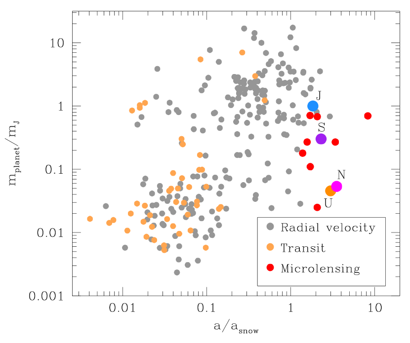
Microlensing provides an important tool to detect multiplanetary systems with cold, wide-orbit planets. There currently exist 1325 planets in 657 known multiplanetary systems by the time of writing this paper. Most of transit planets and majority of RV planets in multiplanetary systems are hot or warm planets located within the snow lines of the systems, and many of these planets are believed to have migrated from the place of their formation to their current locations by various dynamical mechanisms (Lin et al., 1996; Ward, 1997; Murray et al., 1998). Microlensing, on the other hand, is sensitive to cold planets that are likely to have formed in situ and have not undergone large-scale migration, and thus construction of an unbiased sample of planets in this region is important for the investigation of giant planet formation. The high sensitivity of the microlensing method to wide-orbit planets in multiple planetary systems is shown in the distribution of planets on the $a/a_{\rm snow}$–$m_{\rm planet}$ plane presented in Figure 1. Here $a$ and $m_{\rm planet}$ represent the semi-major axis and mass of the planet, respectively. Furthermore, the microlensing method does not rely on the luminosity of the host star. This makes the microlensing method a useful tool for investigating multiplanetary systems with faint host stars, for which the sensitivity of the other methods is low. This is particularly important for probing exoplanet populations, given that M dwarfs are the most common stars in the Galaxy.

Figure 2.— Baseline light curve. The upper and lower panels show 100 day and $\sim 2.2$ year baseline observed by the OGLE survey, respectively.

There exist four reported multiple-planet systems detected using the microlensing method. The first system, OGLE-2006-BLG-109L, is composed of a host with approximately half of the solar mass and two planets with masses of $\sim 0.71~{}M_{\rm J}$ and $\sim 0.27~{}M_{\rm J}$ and orbital separations of $\sim 2.3$ au and $\sim 4.6$ au, and thus the system resembles a scaled version of our solar system in that the mass ratio, separation ratio, and the equilibrium temperatures of the planets are similar to those of Jupiter and Saturn (Gaudi et al., 2008; Bennett et al., 2010). For OGLE-2012-BLG-0026L, two planets with masses of $\sim 0.145~{}M_{\rm J}$ and $\sim 0.86~{}M_{\rm J}$ are orbiting a host star with a mass $\sim 1.06~{}M_{\odot}$ (Han et al., 2013; Beaulieu et al., 2016). For this system, there exist 4 degenerate solutions in the interpretation of the projected planet-host separations, but the separations of the individual planets are beyond the snow line in all solutions, being $\sim 4.0$ au and $\sim 4.8$ au for the best-fit solution. From the statistical arguments and dynamical analysis of the orbital configuration, Madsen & Zhu (2019) argued that the two massive planets in OGLE-2012-BLG-0026L were likely in a resonance configuration. For OGLE-2014-BLG-1722L, two planets with masses of $\sim 0.18~{}M_{\rm J}$ and $\sim 0.27~{}M_{\rm J}$ are orbiting a late-type star with a mass of $\sim 0.4~{}M_{\odot}$. The projected separations from the host are $\sim 1.5$ au for the first planet and $\sim 1.7$ au or $\sim 2.7$ au for the second planet, and thus both planets are also located beyond the snow line (Suzuki et al., 2018). OGLE-2018-BLG-0532L is the most recently reported candidate system, in which two planets with masses of $\sim 8~{}M_{\oplus}$ and $\sim 0.7~{}M_{\rm J}$ are located around an M-dwarf host having a mass of $\sim 0.25~{}M_{\odot}$ with projected separations from the host of $\sim 1.4$ au and 5.6 au, respectively (Ryu et al., 2019). From the detection efficiency analysis of the MOA (Suzuki et al., 2016) and $\mu$FUN (Gould et al., 2010) surveys for the two microlensing multiplanetary systems OGLE-2006-BLG-109L and OGLE-2014-BLG-1722L, Suzuki et al. (2018) estimated that the occurrence rate of systems with multiple cold gas giant systems was $6\%\pm 2\%$. We note that the multiple-planet signatures in the lensing light curves are securely detected for OGLE-2006-BLG-109L and OGLE-2012-BLG-0026L, but the signatures for OGLE-2014-BLG-1722L and OGLE-2018-BLG-0532L are less reliable.

In this paper, we report a new multiple-planet system discovered by analyzing the combined data of the microlensing event OGLE-2018-BLG-1011 obtained by five lensing surveys. We describe data acquisition and processing in Section 2. In Sections 3 through 5, we describe the detailed procedure of analysis leading to the interpretation of the lens as a multiple-planet system. In Sections 6 and 7, we characterize the source of the event and estimate the physical parameters of the lens system, respectively. We summarize the results and conclude in Section 8.

Figure 3.— Light curve of the microlensing event OGLE-2018-BLG-1011. The upper panel shows the enlarged view of the anomaly region around the peak. The curve superposed on the data points is the model curve based on the point-source point-lens interpretation.

2. Observation and Data

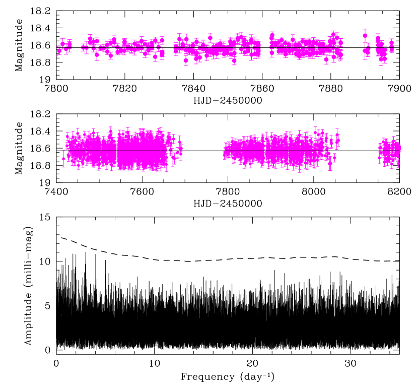
The source star of the microlensing event OGLE-2018-BLG-1011 is located toward the Galactic bulge with equatorial coordinates $({\rm R.A.},{\rm decl.})_{\rm J2000}=(17:56:03.36,-29:04:58.4)$, which correspond to Galactic coordinates of $(l,b)=(1.04^{\circ},-2.04^{\circ})$. In the middle panel of Figure 2, we present the $\sim 2.2$ year baseline light curve observed by the OGLE survey. The top panel, showing the light curve for 100 days during $7800\leq{\rm HJD}^{\prime}\equiv{\rm HJD}-2450000\leq 7900$, is presented to check the short-term variability of the source brightness. It is found that the baseline magnitude, $I_{\rm base}\sim 18.63$, is stable and the light curve does not show noticeable variability. We further investigate the source variability by computing the power spectrum using the PERIOD04 code of Lenz & Breger (2005). The power spectrum is presented in the bottom panel. The dashed line represents the limit with the signal-to-noise ratio ${\rm S/N}=4$, which is the empirically proposed threshold for variability (Breger et al., 1993). The spectrum shows no periodic variability greater than the imposed threshold, indicating that the source flux has been stable.

The brightening of the source star induced by lensing was found in the early rising stage of the event by the Optical Gravitational Lensing Experiment (OGLE: Udalski et al., 2015b), and the discovery was notified to the microlensing community on 2018-06-07 (${\rm HJD}^{\prime}\sim 8277$). The event was in the OGLE-IV BLG505.23 field that was monitored with a cadence of 1 day using the 1.3 m telescope located at the Las Campanas Observatory in Chile. Most OGLE data were acquired in $I$ band, and some $V$-band images were obtained for the source color measurement.

The event was also located in the fields of two other major lensing surveys, namely the Microlensing Observations in Astrophysics (MOA: Bond et al., 2001; Sumi et al., 2003) and Korea Microlensing Telescope Network (KMTNet: Kim et al., 2016). The MOA observations of the event were conducted in a customized broad $R$ band using the 1.8 m telescope located at the Mt. John Observatory in New Zealand. The cadence of the MOA survey was $\sim 10$/night in a survey mode and reached up to 40/night when the anomaly in the lensing light curve was in progress. The event was designated as MOA-2018-BLG-182 in the list of the “MOA Transient Alerts” page.

Figure 4.— $\Delta\chi^{2}$ distribution on the plane of the binary-lensing parameters $s$ and $q$. The color coding indicates points within $1n\sigma$ (red), $2n\sigma$ (yellow), $3n\sigma$ (green), $4n\sigma$ (cyan), $5n\sigma$ (blue), and $6n\sigma$ (purple) with respect to the best-fit value and $n=10$.

The KMTNet survey utilizes three identical 1.6 m telescopes that are globally distributed for continuous coverage of lensing events. The individual telescopes are located at the Siding Spring Observatory in Australia (KMTA), Cerro Tololo Interamerican Observatory in Chile (KMTC), and the South African Astronomical Observatory in South Africa (KMTS). The event was in the two overlapping fields (BLG02 and BLG042) of the KMTNet survey and images were obtained mainly in $I$ band with occasional $V$-band data acquisition. We use $V$-band data not only for the source color measurement but also for the light curve analysis to maximize the coverage of the short-term anomaly that appeared in the peak of the event light curve. The observational cadence of the KMTNet survey varied depending on the observation site, ranging 4/hr for the KMTC telescope and 6/hr for the KMTA and KMTS telescopes. The event was detected by the KMTNet “event finder” (Kim et al., 2018) and was named as KMT-2018-BLG-2122.

Besides the three major microlensing surveys, the event was also observed by two lower-cadence surveys conducted by utilizing the Canada-France-Hawaii Telescope (CFHT) (Zang et al., 2018) and the 3.8 m United Kingdom Infrared Telescope (UKIRT) (Shvartzvald et al., 2017). The CFHT data include 62 points in the time range of $8256\lesssim{\rm HJD}^{\prime}\lesssim 8346$. The UKIRT observations were conducted with a daily cadence in $H$ band and occasional observations in $K$ band. The CFHT data include 62 points obtained during $8256\lesssim{\rm HJD}^{\prime}\lesssim 8346$ and the UKIRT data include 49 $H$-band and 10 $K$-band data points acquired during $7864\lesssim{\rm HJD}^{\prime}\lesssim 8336$ and $7882\lesssim{\rm HJD}^{\prime}\lesssim 8329$, respectively.

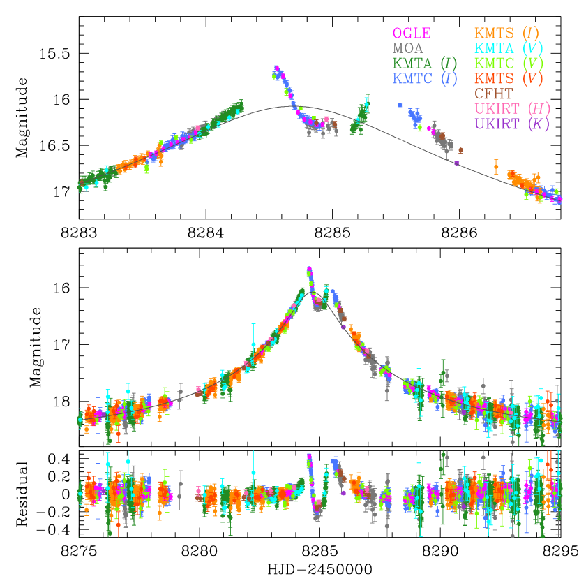
Data sets obtained by the OGLE and MOA surveys were released almost in real time through the “Early Warning System” and “MOA Transient Alerts” pages. This in turn facilitated monitoring of the real-time evolution of the event. On 2018-06-16 (${\rm HJD}^{\prime}\sim 8285.5$), D. Suzuki of the MOA group noticed a deviation of the light curve from a point-source point-lens model and issued an anomaly alert. With this alert, the MOA group increased their observation cadence. See the light curve of the event and the anomaly around the peak presented in Figure 3. The alert triggered real-time analysis of the light curve and a series of models, all of which were based on binary-lens interpretations, were released by V. Bozza, A. Cassan, D. Bennett, and Y. Hirao during the progress of the anomaly. Although results were not circulated, the first author of this paper (C. Han) was also conducting analysis of the event with the progress of the event. When the anomaly ended, however, it was found that none of these models could fully explain the observed anomaly. The fact that the real-time analyses done by five people using separate, independently-written softwares reached the same conclusion that a binary-lens interpretation cannot properly explain the observed data strongly suggests that one needs an interpretation of the event that is different from the binary-lens explanation.

We note that there are gaps in the data during the anomaly despite the coverage by five surveys. The gaps centered at ${\rm HJD}^{\prime}\sim 8284.4$ and 8285.4 could have been covered by KMTS telescope located in Africa and the gap centered at ${\rm HJD}^{\prime}\sim 8286.2$ could have been observed by KMTA telescope located in Australia. Unfortunately, no data could be obtained because of the poor weather conditions of the sites.

Table 1Photometric Uncertainty Rescaling Parameters

Data set	$k$	$\sigma_{0}$ (mag)
OGLE	1.170	0.020
MOA	1.490	0.020
KMTA ($I$, BLG02)	1.523	0.020
KMTA ($I$, BLG42)	2.170	0.020
KMTC ($I$, BLG02)	1.086	0.030
KMTC ($I$, BLG42)	1.584	0.010
KMTS ($I$, BLG02)	1.396	0.020
KMTS ($I$, BLG42)	1.261	0.030
KMTA ($V$, BLG02)	2.017	0.010
KMTA ($V$, BLG42)	2.135	0.010
KMTC ($V$, BLG02)	1.470	0.025
KMTC ($V$, BLG42)	1.421	0.005
KMTS ($V$, BLG02)	1.288	0.010
KMTS ($V$, BLG42)	1.253	0.010
CFHT	0.806	0.040
UKIRT ($H$)	0.500	0.030
UKIRT ($K$)	0.224	0.030

Note. — The notations in the parentheses of the KMTNet data sets represent the passbands and fields of observation.

Table 2Comparison of models

Solution			$\chi^{2}$
2L1S	binary	$s<1.0$	8545.6
		$s>1.0$	8470.6
	planetary	$s<1.0$	8439.7
		$s>1.0$	8477.0
1L2S			10853.6
2L2S			8047.3
3L1S	Planet-binary	$s_{2}<1.0$, $s_{3}<1.0$	7825.4
		$s_{2}<1.0$, $s_{3}>1.0$	7825.5
		$s_{2}>1.0$, $s_{3}<1.0$	7865.2
		$s_{2}>1.0$, $s_{3}>1.0$	7882.9
	Multiple-planet (I)	$s_{2}<1.0$	7783.8
		$s_{2}>1.0$	7790.7
	Multiple-planet (II)	$s_{2}<1.0$, $s_{3}<1.0$	7718.0
		$s_{2}<1.0$, $s_{3}>1.0$	7761.6
		$s_{2}>1.0$, $s_{3}<1.0$	7717.7
		$s_{2}>1.0$, $s_{3}>1.0$	7756.5

Note. — For the 3L1S solutions, $s_{2}$ and $s_{3}$ represent the normalized separation between $M_{1}$–$M_{2}$ and $M_{1}$–$M_{3}$, respectively, and $M_{1}$ represents the primary lens and $M_{2}$ and $M_{3}$ denote the companions.

In our analysis of the event, we use photometry data processed with the codes developed by the individual survey groups: Woźniak (2000) (OGLE), Bond et al. (2001) (MOA) and Albrow (2017) (KMTNet). All of these codes are based on the difference imaging technique of Alard & Lupton (1998). For a subset of KMTNet data, additional photometry is processed using the pyDIA photometry (Albrow, 2017) to measure the source color. For the use of multiple data sets obtained by different groups and processed by using different photometry codes, we normalize the photometric measurement uncertainties of the data sets following the procedure of Yee et al. (2012), in which the photometric uncertainties are rescaled by

$$\sigma=k(\sigma_{0}^{2}+\sigma_{\rm min}^{2})^{1/2}.$$ (1)

The quadratic term $\sigma_{0}$ is added so that the cumulative distribution of $\chi^{2}$ ordered by magnification is approximately linear. This process ensures the dispersion of data points consistent with error bars. The coefficient “$k$” is a factor used for rescaling the errors so that $\chi^{2}$ per degree of freedom ($\chi^{2}/{\rm dof}$) for each data set becomes unity. The latter process is needed to prevent each data set from being under or over-represented compared to other data sets. In Table 1, we present the values of $k$ and $\sigma_{0}$.

Table 3Lensing parameters of 2L1S, 1L2S, and 2L2S models

Parameter	2L1S (Binary)		2L1S (Planet)		1L2S	2L2S
	($s<1$)	($s>1$)	($s<1$)	($s>1$)
$\chi^{2}$	8546.6	8470.6	8439.7	8477.0	10853.6	8047.3
$t_{0,1}$ (${\rm HJD}^{\prime}$)	$8284.605\pm 0.003$	$8284.594\pm 0.002$	$8284.751\pm 0.003$	$8284.755\pm 0.003$	$8284.439\pm 0.004$	$8284.646\pm 0.004$
$u_{0,1}$	$0.032\pm 0.001$	$0.022\pm 0.001$	$0.062\pm 0.001$	$0.063\pm 0.001$	$0.061\pm 0.001$	$0.063\pm 0.001$
$t_{0,2}$ (${\rm HJD}^{\prime}$)	–	–	–	–	$8285.686\pm 0.011$	$8285.403\pm 0.007$
$u_{0,2}$	–	–	–	–	$0.027\pm 0.001$	$0.011\pm 0.001$
$t_{\rm E}$ (days)	$12.73\pm 0.15$	$17.53\pm 0.25$	$10.61\pm 0.11$	$10.58\pm 0.11$	$12.69\pm 0.16$	$11.05\pm 0.08$
$s$	$0.338\pm 0.003$	$5.097\pm 0.070$	$0.807\pm 0.004$	$1.169\pm 0.006$	–	$0.784\pm 0.002$
$q$	$0.301\pm 0.015$	$1.108\pm 0.096$	$(6.98\pm 0.15)\times 10^{-3}$	$(7.03\pm 0.17)\times 10^{-3}$	–	$(6.61\pm 0.09)\times 10^{-3}$
$\alpha$ (rad)	$0.246\pm 0.005$	$0.235\pm 0.005$	$4.434\pm 0.005$	$4.440\pm 0.005$	–	$4.253\pm 0.008$
$\rho_{1}$ ($10^{-3}$)	–	–	–	–	–	–
$\rho_{2}$ ($10^{-3}$)	–	–	–	–	$7.58\pm 3.07$	$0.80\pm 0.13$
$q_{F,I}$	–	–	–	–	$0.24\pm 0.01$	$0.071\pm 0.003$

Note. — ${\rm HJD}^{\prime}={\rm HJD-2450000}$.

3. Binary-lens (2L1S) interpretations

The light curve of the event exhibits an anomaly that is characterized by two bumps near the peak. We start the analysis of the anomaly with the “2L1S” interpretation, in which the event is produced by a lens composed of two masses, “2L,” deflecting the light from a single source, “1S.”

It is known that a double-bump feature in the peak region of a lensing light curve can be produced by two major channels of 2L1S events (Han & Gaudi, 2008). One channel is the case, in which the source trajectory approaches the two neighboring cusps of the central caustic produced by a binary lens composed of similar masses with a projected separation between the lens components significantly smaller (close binary) or wider (wide binary) than the Einstein radius $\theta_{\rm E}$ of the lens system. The other channel is the case, in which the source approaches the back-end cusp of the central caustic produced by a planetary lens system with a mass ratio between the lens components $q\ll 1$ and a star-planet separation similar to $\theta_{\rm E}$ (Choi et al., 2012; Park et al., 2014; Bozza et al., 2016). We refer to the former and latter channels as the “binary” and “planetary” channels, respectively.

Figure 5.— Model light curves of the two solutions obtained for the 2L1S interpretation: binary (blue curve: $s<1.0$ (close solution); cf., Table 3) and planetary (red curve: $s<1.0$ close solution); cf., Table 3) solutions. The two lower panels show the residuals from the individual models. The lens-system configurations corresponding to the individual solutions are presented in Fig. 6.

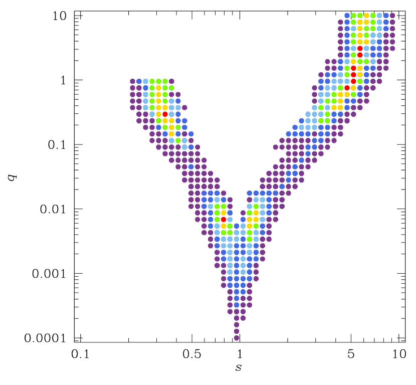
For the 2L1S analysis, we first conduct a dense grid search for the lensing parameters $s$ and $q$, which represent the binary separation normalized to $\theta_{\rm E}$ and the mass ratio between the lens components, respectively. Considering that central perturbations can be produced either by a planetary companion with a low mass ratio or a binary companion with very wide or close separations from the primary, we set the ranges of $s$ and $q$ for the grid search wide enough to check both the planetary and binary solutions. The initial grid search is done in the ranges of $-1.0\leq\log s\leq 1.0$ and $-4.0\leq\log q\leq 1.0$ for the separation and mass ratio, respectively, with 50 grids for each range. We then identify local minima in the distribution of $\Delta\chi^{2}$ on the $s$–$q$ plane. For the individual local solutions, we gradually narrow down the ranges of the parameter space in the grid search. Besides these lensing parameters, a basic 2L1S modeling requires additional parameters, including the time of the closest lens-source approach, $t_{0}$, the lens-source separation at that time, $u_{0}$ (normalized to $\theta_{\rm E}$), the Einstein timescale, $t_{\rm E}$, and the source trajectory angle with respect to the binary-lens axis, $\alpha$. In the case when the source crosses the caustic formed by the binary lens, the lensing light curve is affected by finite-source effects and one needs an additional parameter of $\rho$, which represents the source radius $\theta_{*}$ normalized to $\theta_{\rm E}$, i.e., $\rho=\theta_{*}/\theta_{\rm E}$, to account for these effects. (MCMC) method. In computing finite-source magnifications, we consider surface-brightness variation of the source stars caused by the limb darkening. The stellar type of the source turns out to be a G-type turn-off star (Section 6) and thus we adopt a linear limb-darkening coefficient of $\Gamma_{I}=0.5$. For a given set of $(s,q)$, we search for the other lensing parameters using a downhill approach based on the Markov Chain Monte Carlo (MCMC) method.

In Figure 4, we present the distribution of $\Delta\chi^{2}$ from the best-fit model on the $s$–$q$ parameter plane obtained from the initial grid search. We find that there exist four local solutions. For one pair of the local solutions, the mass ratios are $q\sim 1$, and thus the solutions correspond to binary-lens solutions. For the other pair, the mass ratios are $q<10^{-2}$, indicating that they correspond to planetary mass lens solutions. For each pair, we find that there exist two solutions with $s<1$ (close solution) and $s>1$ (wide solution), which are generated by the close/wide degeneracy (Griest & Safazadeh, 1998; Dominik, 1999).

Figure 6.— Lens-system configurations of the 2L1S solutions. The upper and lower panels correspond to the “binary” (with $s<1.0$) and “planetary” (with $s<1.0$) solutions, respecively. In each panel, the line with an arrow represents the source trajectory and the red close curve is the caustic. The blue dots marked by $M_{1}$ and $M_{2}$ denote the positions of the binary lens components.

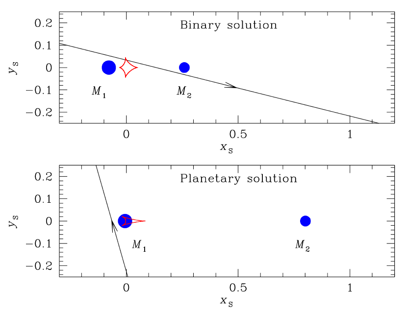
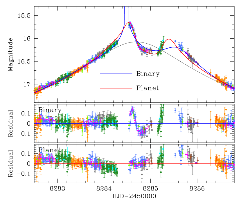
In Figure 5, we present the model light curves corresponding to the “binary” (blue curve) and “planetary” (red curve) 2L1S solutions superposed on the observed data, together with the residuals from the models (presented in the lower two panels). We note that the individual solutions are further refined based on the local minima obtained from the grid search by allowing all lensing parameters, including $s$ and $q$, to vary. In Table 2, we compare the $\chi^{2}$ values of the four 2L1S solutions. In Table 3, we list the best-fit lensing parameters of the individual 2L1S solutions. We also note that the model light curves corresponding to the close and wide solutions of each of the binary and planetary solution pairs are similar to each other and thus in Figure 5 we present the one yielding a better fit to the data. In Figure 6, we present the lens-system configurations, which represent the source trajectory with respect to the caustic, of the binary (upper panel) and planetary (lower panel) solutions. We note that the presented configurations are for the close ($s<1.0$) solutions. From the fits of the individual models to the observed data, it is found that the binary-lens solution leaves substantial residuals in the region $8284.5\lesssim{\rm HJD}^{\prime}\lesssim 8285.6$, and the planetary solution leaves residuals in the region $8285.6\lesssim{\rm HJD}^{\prime}\lesssim 8286.0$. These residuals indicate that neither the binary nor the planetary 2L1S solutions adequately describe the observed data and suggest that a new interpretation of the light curve is required.

We additionally check whether the fit further improves by considering the microlens-parallax (Gould, 1992) and/or the lens-orbital (Dominik, 1998; Ioka et al., 1999) effects. It is found that the improvement by these higher-order effects is negligible, mainly due to the short timescale, $t_{\rm E}\sim 12$ days, of the event.

Table 4Lensing parameters of “planet-binary” 3L1S solutions

Parameter	$s_{2}<1.0$, $s_{3}<1.0$	$s_{2}<1.0$, $s_{3}>1.0$	$s_{2}>1.0$, $s_{3}<1.0$	$s_{2}>1.0$, $s_{3}>1.0$
$\chi^{2}$	7825.4	7825.5	7865.2	7882.9
$t_{0}$ (${\rm HJD}^{\prime}$)	8284.557 $\pm$ 0.006	8284.564 $\pm$ 0.005	8284.557 $\pm$ 0.004	8284.549 $\pm$ 0.003
$u_{0}$	0.033 $\pm$ 0.001	0.034 $\pm$ 0.001	0.023 $\pm$ 0.001	0.023 $\pm$ 0.001
$t_{\rm E}$ (days)	12.80 $\pm$ 0.14	12.70 $\pm$ 0.15	17.12 $\pm$ 0.20	16.59 $\pm$ 0.12
$s_{2}$	0.357 $\pm$ 0.004	0.354 $\pm$ 0.004	4.872 $\pm$ 0.073	4.559 $\pm$ 0.039
$q_{2}$	0.263 $\pm$ 0.012	0.273 $\pm$ 0.012	0.977 $\pm$ 0.079	0.703 $\pm$ 0.035
$\alpha$ (rad)	0.282 $\pm$ 0.0054	0.283 $\pm$ 0.005	0.268 $\pm$ 0.004	0.265 $\pm$ 0.004
$s_{3}$	0.812 $\pm$ 0.015	1.262 $\pm$ 0.023	0.896 $\pm$ 0.025	1.002 $\pm$ 0.006
$q_{3}$	$(2.81\pm 0.45)\times 10^{-3}$	$(2.28\pm 0.46)\times 10^{-3}$	$(1.71\pm 0.26)\times 10^{-3}$	$(2.28\pm 0.26)\times 10^{-3}$
$\psi$ (rad)	1.259 $\pm$ 0.006	1.299 $\pm$ 0.005	1.371 $\pm$ 0.005	1.361 $\pm$ 0.004

Note. — ${\rm HJD}^{\prime}={\rm HJD-2450000}$.

4. Binary-source (1L2S and 2L2S) Interpretation

Gaudi (1998) pointed out the possibility that a short-term perturbation, which was the main feature of a planetary microlensing signal produced by major-image perturbations, could be reproduced by a subset of binary-source events, in which a single-mass lens, 1L, passed close to the fainter member of the binary source, 2S. The degeneracy between 2L1S and 1L2S interpretations can often be severe, as demonstrated in the cases OGLE-2002-BLG-055 (Gaudi & Han, 2004), MOA-2012-BLG-486 (Hwang et al., 2013), and OGLE-2014-BLG-1186 (Dominik et al., 2019). Besides the short-term anomaly considered by Gaudi (1998), it was shown that the 2L1S/1L2S degeneracy could extend to various cases of planetary lens system configurations from the analysis of anomalies in the cases of OGLE-2016-BLG-0733 by Jung et al. (2017) and KMT-2017-BLG-0962 and KMT-2017-BLG-1119 by Shin et al. (2019).

Figure 7.— Model light curves obtained for the 1L2S (dotted curve) and 2L2S (solid curve) interpretations. The two lower panels show the residuals of the individual models. The inset in the top panel shows the lens-system configuration of the 2L2S solution. The black lines with arrows marked by “${\rm S}_{1}$” and “${\rm S}_{2}$” represent the trajectories (lines with arrows) of the binary-source components with respect to the caustic (red closed figure).

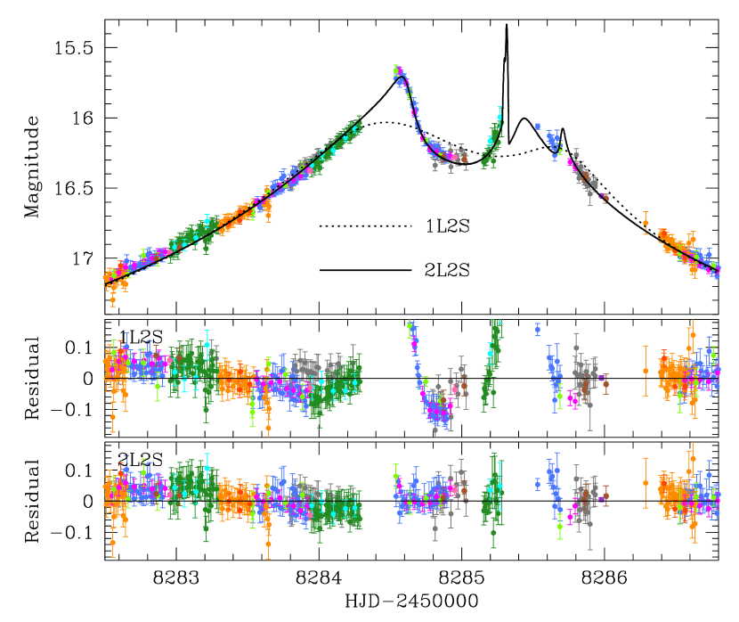
We check the binary-source interpretation of the anomaly in the light curve of OGLE-2018-BLG-1011 by conducting a 1L2S modeling of the observed light curve. The addition of the source companion requires the inclusion of additional parameters in modeling. These parameters are $t_{0,2}$, $u_{0,2}$, and $q_{F}$, which represent the time of the closest lens approach to the source companion, the impact parameter to the companion, and the flux ratio between the source stars, respectively. We note that finite-source effects are considered in the modeling. From this modeling, we find that the 1L2S solution provides a poorer fit than the best-fit 2L1S solutions, by $\Delta\chi^{2}=2313.1$ and $2418.9$ compared to the binary and planetary 2L1S solutions, respectively, and thus we reject the solution. In Figure 7, we present the best-fit 1L2S model (dotted curve superposed on the data points).

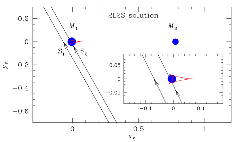
We also check the model in which both the source and lens are binaries, 2L2S model. Figure 7 shows the model light curve (solid curve) of the best-fit 2L2S solution. In Figure 8, we also present the lens-system configuration corresponding to the model. We note that there are two source trajectories because the source is a binary in the 2L2S model. The solution provides a better fit than the 2L1S and 1L2S solutions, but it leaves noticeable residuals in the region $8282.5\lesssim{\rm HJD}^{\prime}\lesssim 8283.2$. As we will show in the following section, the fit of the 2L2S solution is worse than the best-fit solution based on other interpretation by $\Delta\chi^{2}=329.6$. In Table 2, we list the $\chi^{2}$ values of the 1L2S and 2L2S solutions. In Table 3, we also list the best-fit lensing parameters of the 1L2S and 2L2S solutions.

Figure 8.— Lens-system configuration of the best-fit 2L2S model. Notations are same as those in Fig. 6 except that there are two source trajectories because the source is a binary. The trajectories marked by $S_{1}$ and $S_{2}$ represent those of the brighter and fainter source stars, respectively.

5. Triple-lens (3L1S) Interpretation

Knowing the inadequacy of the 2L1S, 1L2S, and 2L2S solutions in describing the observed light curve, we then model the light curve assuming a triple-lens interpretation, in which the lens contains 3 components, 3L. We try 3L1S modeling because the solutions obtained from the 2L1S modeling partially describe the observed central perturbation and the residual from the 2L1S model may be explained by introducing an additional lens component.

Central perturbations of lensing light curves in 3L1S cases can be produced through two major channels. One channel is through multiple-planet systems, in which the individual planets located in the lensing zone can affect the magnification pattern of the central perturbation region (Gaudi et al., 1998). Among the four known multiplanetary systems detected by microlensing, three systems, OGLE-2006-BLG-109Lb,c, OGLE-2012-BLG-0026Lb,c, and OGLE-2018-BLG-0532Lab, were detected through the central perturbations induced by two planets. The other channel is through planet+binary systems. Similar to the central caustic produced by a planet, a very close or a very wide binary companion can also induce a small caustic in the central magnification region and thus can affect the magnification pattern. Among the four known microlensing planetary systems in binaries, the circumbinary planetary system OGLE-2007-BLG-349L(AB)c was detected through this channel.

The lensing behavior of triple-lens systems is qualitatively different from that of binary-lens systems, resulting in a complex caustic structure, such as nested caustic and self-intersections. The range of the critical-curve topology and the caustic structure of the triple lens has not yet been fully explored, making it difficult to analyze triple-lens events (Daněk & Heyrovský, 2015, 2019). As a result, there are some events suspected to be triple-lens events, but plausible models have yet not been proposed, e.g., OGLE-2008-BLG-270, OGLE-2012-BLG-0442/MOA-2012-BLG-245, OGLE-2012-BLG-0207/MOA-2012-BLG-105, and OGLE-2018-BLG-0043/MOA-2018-BLG-033. In some cases, interpretations of triple-lens events can be confused with those of binary-lens events, as in the cases of MACHO-97-BLG-41 (Bennett et al., 1999; Albrow et al., 2000; Jung et al., 2013) and OGLE-2013-BLG-0723 (Udalski et al., 2015a; Han et al., 2016).

Despite the diversity and complexity of the lensing behavior, triple-lens events can be readily analyzed for some specific lens cases. One such a case occurs when the lens companions produce small perturbations with minor interference in the magnification pattern between the perturbations produced by the individual companions. In this case, the resulting anomaly can be approximated by the superposition of the two binary anomalies, in which the individual primary-companion pairs act as independent 2-body systems (Han, 2005). This binary-superposition approximation can be applied for two cases of triple-lens systems, in which the lens is composed of multiple planets, as demonstrated in the cases of OGLE-2006-BLG-109 (Gaudi et al., 2008) OGLE-2012-BLG-0026 (Han et al., 2013), and planets in close or wide binary systems, as demonstrated in the case of OGLE-2016-BLG-0613 (Han et al., 2017). The 2L1S modeling of OGLE-2018-BLG-1011 yields two local solutions, with a planetary companion and a close/wide binary companion, respectively. This suggests that the event may be the case for which the analysis based on the superposition approximation is valid.

Figure 9.— $\Delta\chi^{2}$ map in the $s_{3}$–$q_{3}$ parameter plane obtained from the grid search with the initial values of the “planetary” 2L1S solution. The local marked by the empty triangle dot corresponds to the “multiple-planet (I)” solution and the two locals marked by the empty square dots corresponds to the “multiple-planet (II)” solutions. The color coding is same as that of Fig. 4.

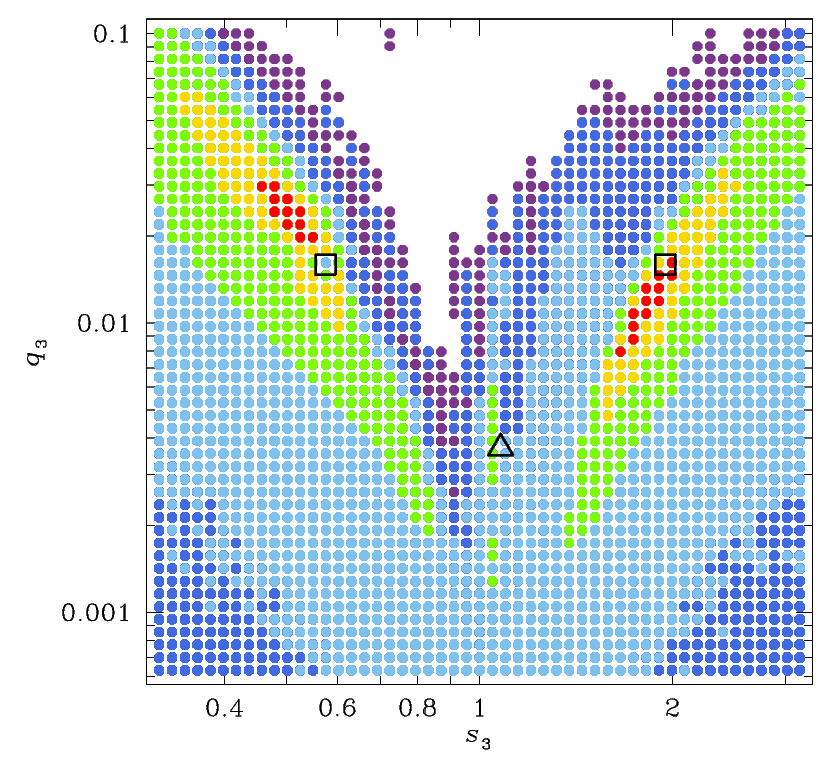
The 3L1S modeling is done in two steps. In the first step, we conduct a grid search for the separation $s_{3}$ and mass ratio $q_{3}$ between $M_{1}$ and $M_{3}$, and the orientation angle $\psi$ of the third body with respect to the $M_{1}$–$M_{2}$ axis. Here, we use the subscripts “1”–“3” to denote the individual lens components. In this search, we fix the values of ($s_{2},q_{2},\alpha)$ as those obtained from the 2L1S modeling. Because two local 2L1S solutions are found, i.e., the “binary” and “planetary” solutions, we conduct two sets of modeling with the initial values of $(s_{2},q_{2},\alpha)$ of the “binary” and “planetary” solutions obtained from the 2L1S modeling. We use the parameters of the close 2L1S solution as the initial parameters, but the result would not be affected with the use of the wide solution parameters because of the similarity between the model light curves of the close and wide solutions. In Figure 9, we present the $\Delta\chi^{2}$ map in the $s_{3}$–$q_{3}$ parameter plane obtained from the grid search with the initial values of the “planetary” 2L1S solution. In the second step, we refine the solutions found from the grid search by allowing all parameters to vary.

Figure 10.— Model light curves of the three solutions obtained for the 3L1S interpretation: “planet-binary” (blue curve: $s_{2}<1,s_{3}<1$; cf., Table 4), “multiple-planet (I)” (red curve: $s_{2}<1$; cf., Table 5), “multiple-planet (II)” (black curve: $s_{2}>1,s_{3}<1$; cf., Table 6). The three lower panels show the residuals from the individual models. The upper left inset in the top panel shows the enlarged view of the source star’s cusp approach at around ${\rm HJD}^{\prime}\sim 8283.0$ according to the “multiple-planet (I)” solution, and the lower middle inset shows the zoom of the caustic-crossing region according to the “planet-binary” solution.

Figure 11.— Lens-system configuration of the “planet-binary” 3L1S solution with $s_{2}<1.0$ and $s_{3}<1.0$. The blue dots marked by $M_{1}$, $M_{2}$, and $M_{3}$ represent the locations of the three lens components. The inset shows the enlargement of the central caustic region. We note that the central caustic structures of the other three degenerate solutions presented in Table 4 are similar to the presented one.

The 3L1S modeling yields three sets of solutions. One set of solutions results from the starting values of $(s_{2},q_{2},\alpha)$ of the binary 2L1S solution and the other two sets result from the starting $(s_{2},q_{2},\alpha)$ values of the planetary 2L1S solution. The solutions found based on the binary 2L1S solution indicates that the lens is a planetary system in a binary. We designate these solutions as the “planet-binary” solutions. The two sets of solutions found based on the planetary 2L1S solution indicate that the lens is a multiplanetary system. We designate these two sets of solutions as the “multiple-planet (I)” and “multiple-planet (II)” solutions. For all 3L1S solutions, the fits greatly improve with respect to the 2L1S and 1L2S models and the gross features of the anomalies are better described. In Table 2, we list the $\chi^{2}$ values of the individual solutions. We discuss the details of the individual solutions in the following subsections.

5.1. Planet-binary solution

We find the “planet-binary” 3L1S solutions from the modeling using the initial values of $(s_{2},q_{2},\alpha)$ obtained from the “binary” 2L1S solution. We find four degenerate solutions resulting from the close/wide degeneracy in the separations between $M_{1}$–$M_{2}$ ($s_{2}<1.0$ and $s_{2}>1.0$) and $M_{1}$–$M_{3}$ ($s_{3}<1.0$ and $s_{3}>1.0$) pairs. In Table 4, we list the lensing parameters of the individual solutions along with $\chi^{2}$ values. It is found that the solutions with $s_{2}<1.0$ are preferred over the solutions with $s_{2}>1.0$ by $\Delta\chi^{2}\gtrsim 40$. For the two solutions with $s_{2}<1.0$, however, the degeneracy between the solutions with $s_{3}<1.0$ and $s_{3}>1.0$ is very severe, i.e., $\Delta\chi^{2}\sim 0.5$.

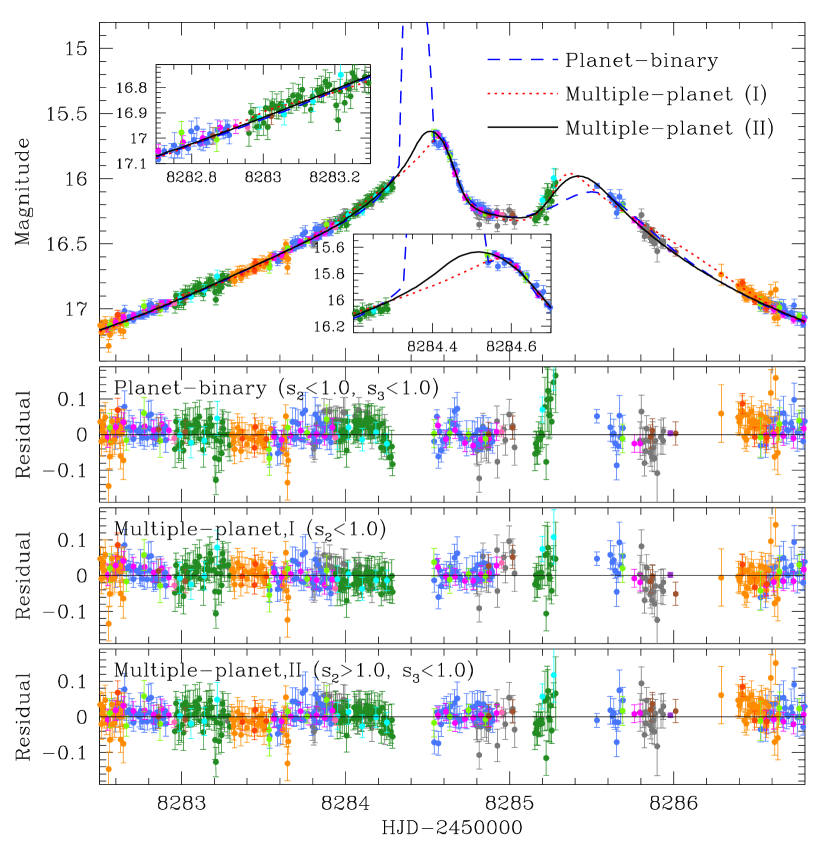
In Figure 10, we present the model light curve (blue dashed curve) of the best-fit planet-binary solution (with $s_{2}<1.0$ and $s_{3}<1.0$) and the residual from the model. In Figure 11, we also present the lens-system configuration corresponding to the solution. We note that the central caustic structures of the other degenerate solutions are similar to the presented one. According to the planet-binary solutions, the source trajectory passed the upper tip of the central caustic, producing two caustic-crossing spikes at ${\rm HJD}^{\prime}\sim 8284.3$ (caustic entrance) and 8284.5 (caustic exit), but the crossings happened in the region of the data ending just before the caustic entrance and starting just after the caustic exit. See the enlarge view of the crossing-crossing region of the light curve presented in the lower middle inset of the top panel in Figure 10. As a result, the value of the normalized source radius $\rho$ cannot be securely measured and its value is not presented in Table 4.

Figure 12.— Lens-system configuration of the “multiple-planet (I)” 3L1S solution with $s_{2}<1.0$. Notations are same as those in Fig. 11. The three “X” marks in the inset represent the source positions at the times of the cusp approaches at $t_{1}=8284.6$, $t_{2}=8285.4$, and $t^{\prime}=8283.0$.

By comparing the lens-system configuration of the “planet-binary” 3L1S solution (presented in Figure 11) with that of the “binary” 2L1S solution (presented in the upper panel in Figure 6), one finds that a tiny wedge-shape caustic appears due to the additional planetary companion with a mass ratio of $q_{3}\sim(1.7-2.8)\times 10^{-3}$. From the comparison with the “binary” 2L1S model (presented in Figure 5), it is found that the introduction of the third body substantially reduces the residuals of the 2L1S solution in the region $8284.5\lesssim{\rm HJD}^{\prime}\lesssim 8285.1$ and improves the fit by $\Delta\chi^{2}\sim 645$. We find that the fit improvement by the microlens-parallax and lens-orbital effects is negligible.

Table 5Lensing parameters of “multiple-planet (I)” 3L1S solutions

Parameter	$s_{2}<1.0$	$s_{2}>1.0$
$\chi^{2}$	7783.8	7790.7
$t_{0}$ (${\rm HJD}^{\prime}$)	8284.761 $\pm$ 0.004	8284.756 $\pm$ 0.004
$u_{0}$	0.070 $\pm$ 0.001	0.072 $\pm$ 0.001
$t_{\rm E}$ (days)	10.30 $\pm$ 0.11	10.37 $\pm$ 0.11
$s_{2}$	0.786 $\pm$ 0.003	1.193 $\pm$ 0.005
$q_{2}$ $(10^{-3})$	6.47 $\pm$ 0.14	6.60 $\pm$ 0.16
$\alpha$ (rad)	4.424 $\pm$ 0.006	4.424 $\pm$ 0.006
$s_{3}$	1.078 $\pm$ 0.005	1.076 $\pm$ 0.004
$q_{3}$ $(10^{-3})$	3.70 $\pm$ 0.15	3.75 $\pm$ 0.14
$\psi$ (rad)	5.175 $\pm$ 0.006	5.174 $\pm$ 0.006

Note. — ${\rm HJD}^{\prime}={\rm HJD-2450000}$.

5.2. Multiple-planet (I) solution

The “multiple-planet (I)” 3L1S solution set is one of the two sets of solutions obtained using the starting values of $(s_{2},q_{2},\alpha)$ from the “planetary” 2L1S solution. For this set of solutions, we find two degenerate solutions caused by the close/wide degeneracy in estimating the $M_{1}$–$M_{2}$ separation, $s_{2}$. The projected separation between $M_{1}$ and $M_{3}$ is very close to unity, $s_{3}\sim 1.08$, and thus there is no close/wide degeneracy in estimating $s_{3}$. It is found that the solution with $s_{2}<1.0$ is slightly preferred over the solution with $s_{2}>1.0$ by $\Delta\chi^{2}=6.9$. Both companions $M_{2}$ and $M_{3}$ have planetary mass ratios of $q_{2}\sim 6.5\times 10^{-3}$ and $q_{3}\sim 3.7\times 10^{-3}$, respectively, indicating that the lens is a multiplanetary system composed of two giant planets. In Table 5, we list the lensing parameters for both solutions with $s_{2}<1.0$ and $s_{2}>1.0$. The “multiple-planet (I)” solution with $s<1.0$ provides a better fit than the planetary planetary 2L1S solution by $\Delta\chi^{2}=555.9$.

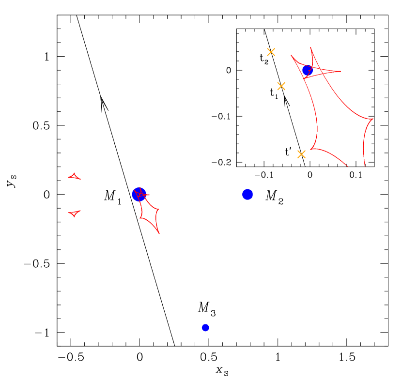
In Figure 10, we plot the model light curve of the “multiple-planet (I)” solution with $s_{2}<1.0$ (red dotted curve) and the residuals from the model. In Figure 12, we also present the lens-system configurations corresponding to the solution. It is found that the third body $M_{3}$ induces a resonant caustic in the central magnification region in addition to the central caustic induced by $M_{2}$. We note that the solution with $s_{2}>1.0$ results in a similar central caustic. In the inset of Figure 12, we mark the positions of the source corresponding to the two major bumps at $t_{1}={\rm HJD}^{\prime}\sim 8284.6$ and $t_{2}\sim 8285.4$. It is found the first bump at $t_{1}$ is produced when the source approaches the back-end cusp of the caustic induced by $M_{2}$, while the second bump at $t_{2}$ is produced by the source approach close to one of the back-end cusps of the caustic induced by $M_{3}$. We note that the source approaches another cusp induced by $M_{3}$ at the position marked by $t^{\prime}\sim 8283.0$ in the inset of Figure 12. This approach also produces a bump, although the bump is weak. See the upper left inset in the top panel of Figure 10. We note that, unlike the binary-planet solution, the “multiple-planet (I)” solution explains the anomaly without a caustic-crossing feature. As a result, and similarly to the binary-planet solution, the normalized source radius $\rho$ cannot be measured and it is not presented in Table 5. Similar to the case of the binary-planet solution, the higher-order effects are not important for the description of the observed light curve.

Table 6Lensing parameters of “multiple-planet (II)” 3L1S solutions

Parameter	$s_{2}<1.0$, $s_{3}<1.0$	$s_{2}<1.0$, $s_{3}>1.0$	$s_{2}>1.0$, $s_{3}<1.0$	$s_{2}>1.0$, $s_{3}>1.0$
$\chi^{2}$	7718.0	7761.6	7717.7	7756.5
$t_{0}$ (${\rm HJD}^{\prime}$)	8284.818 $\pm$ 0.005	8284.868 $\pm$ 0.009	8284.801 $\pm$ 0.005	8284.851 $\pm$ 0.009
$u_{0}$	0.049 $\pm$ 0.001	0.047 $\pm$ 0.001	0.053 $\pm$ 0.001	0.052 $\pm$ 0.001
$t_{\rm E}$ (days)	12.19 $\pm$ 0.14	12.41 $\pm$ 0.21	12.42 $\pm$ 0.15	12.53 $\pm$ 0.21
$s_{2}$	0.750 $\pm$ 0.005	0.747 $\pm$ 0.007	1.281 $\pm$ 0.009	1.276 $\pm$ 0.011
$q_{2}$ ($10^{-3}$)	9.25 $\pm$ 0.21	9.73 $\pm$ 0.30	9.84 $\pm$ 0.26	10.22 $\pm$ 0.37
$\alpha$ (rad)	4.361 $\pm$ 0.008	4.433 $\pm$ 0.008	4.360 $\pm$ 0.008	4.430 $\pm$ 0.008
$s_{3}$	0.577 $\pm$ 0.005	1.954 $\pm$ 0.048	0.582 $\pm$ 0.005	1.929 $\pm$ 0.047
$q_{3}$ ($10^{-3}$)	15.24 $\pm$ 0.59	16.06 $\pm$ 1.70	15.00 $\pm$ 0.61	15.70 $\pm$ 1.76
$\psi$ (rad)	4.859 $\pm$ 0.010	4.733 $\pm$ 0.011	4.858 $\pm$ 0.009	4.740 $\pm$ 0.011
$\rho$ ($10^{-3}$)	11.26 $\pm$ 0.72	11.29 $\pm$ 0.76	12.13 $\pm$ 0.71	11.72 $\pm$ 0.75

Note. — ${\rm HJD}^{\prime}={\rm HJD-2450000}$.

Figure 13.— Lens-system configuration of the “multiple-planet (II)” 3L1S solution with $s_{2}>1.0$ and $s_{3}<1.0$. Notations are same as those in Figure 11. The small empty circle in the inset represents the source and it is presented to show the scaled size of the source relative to the caustic.

Figure 14.— Magnification pattern around the central caustic of the “multiple-planet (II)” solution with $s_{2}>1.0$ and $s_{3}<1.0$. The innermost contour is drawn at $A=50$ and the other contours are drawn at the descending magnifications with a step $\Delta A=2$ from the center toward outward. The two empty circles represent the source locations at the times of the two major bumps at $t_{1}=8284.6$ and $t_{2}=8285.4$, and the size of the circle is scaled to the source size.

5.3. Multiple-planet (II) solution

For given $(s_{2},q_{2},\alpha)$ values of the “planetary” 2L1S solution, we find another set of 3L1S solutions. We designate these solutions as the “multiple-planet (II)” solutions. The mass ratios between $M_{1}$ and $M_{3}$ of the “multiple-planet (II)” solutions is $q_{3}\sim 15\times 10^{-3}$, which is considerably bigger than mass ratios of the “multiple-planet (I)” solutions of $\sim 3.7\times 10^{-3}$. In addition, the $M_{1}$–$M_{3}$ separations of the “multiple-planet (II)” solutions are substantially different from unity, while the $s_{3}$ values of the “multiple-planet (I)” solutions are close to unity. The best-fit “multiple-planet (II)” solution (with $s_{2}>1.0$ and $s_{3}<1.0$) yields a better fit to the observed data than the planetary 2L1S solution by $\Delta\chi^{2}=722.0$.

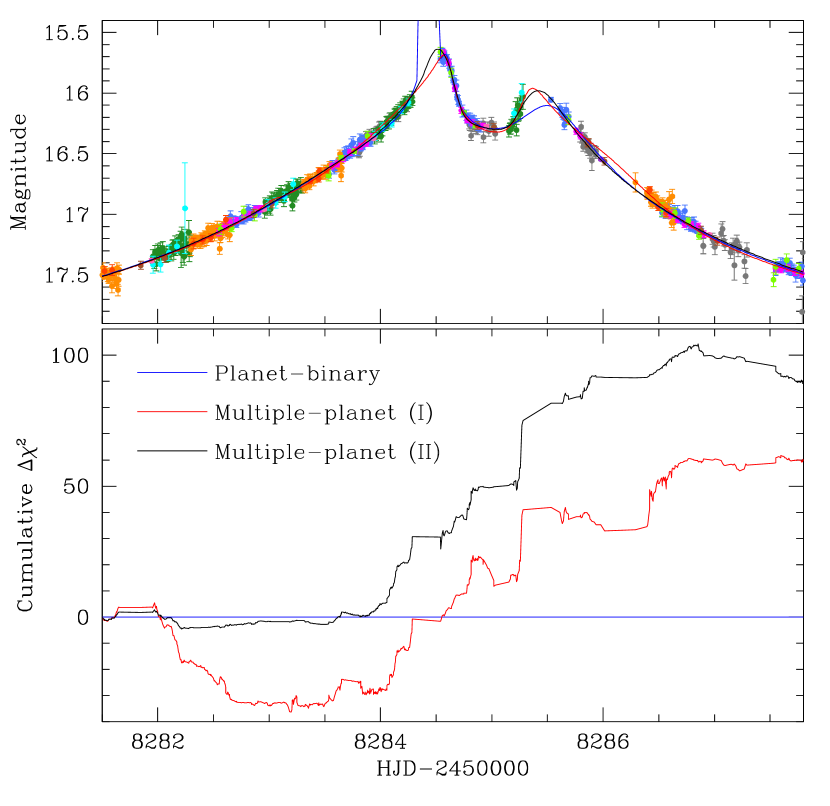
In Table 6, we list the lensing parameters of the “multiple-planet (II)” solutions. We find that there exist 4 solutions resulting from the close/wide degeneracies in both $s_{2}$ and $s_{3}$. From the comparison of the $\chi^{2}$ values of the individual solutions, it is found that the solutions with $s_{3}<1.0$ is favored over the solutions with $s_{3}>1.0$ by $\Delta\chi^{2}\sim 40$. However, the two solutions resulting from the close/wide degeneracy in $s_{2}$ is very severe with $\Delta\chi^{2}=0.3$. In Figure 10, we present the model light curve of the solution with $s_{2}>1.0$ and $s_{3}<1.0$, which yields the best-fit to the data, and the residual from the model.

Figure 15.— Distribution of points in the MCMC chain on the $u_{0}$–$\rho$ plane. The red, yellow, green, cyan, and blue colors represent points with $1\sigma$, $2\sigma$, $3\sigma$, $4\sigma$, and $5\sigma$, respectively.

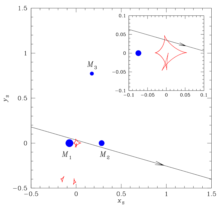
In Figure 13, we present the lens-system configuration of the best-fit “multiple-planet (II)” solution. The central caustic appears to be the superposition of the two sets of central caustics induced by the $M_{1}$–$M_{2}$ and $M_{1}$–$M_{3}$ 2-body lens pairs. According to this solution, the bumps at $t_{1}$ and $t_{2}$ are produced by the successive approaches of the source close to the back-end cusps of the central caustic produced by the $M_{1}$–$M_{2}$ binary pair. However, the cusp of the first source approach is deformed by $M_{3}$ and thus the central caustic is different from that of the central caustic of the $M_{1}$–$M_{2}$ binary. We note that the patterns of central caustics for the other degenerate solutions are similar to the presented one.

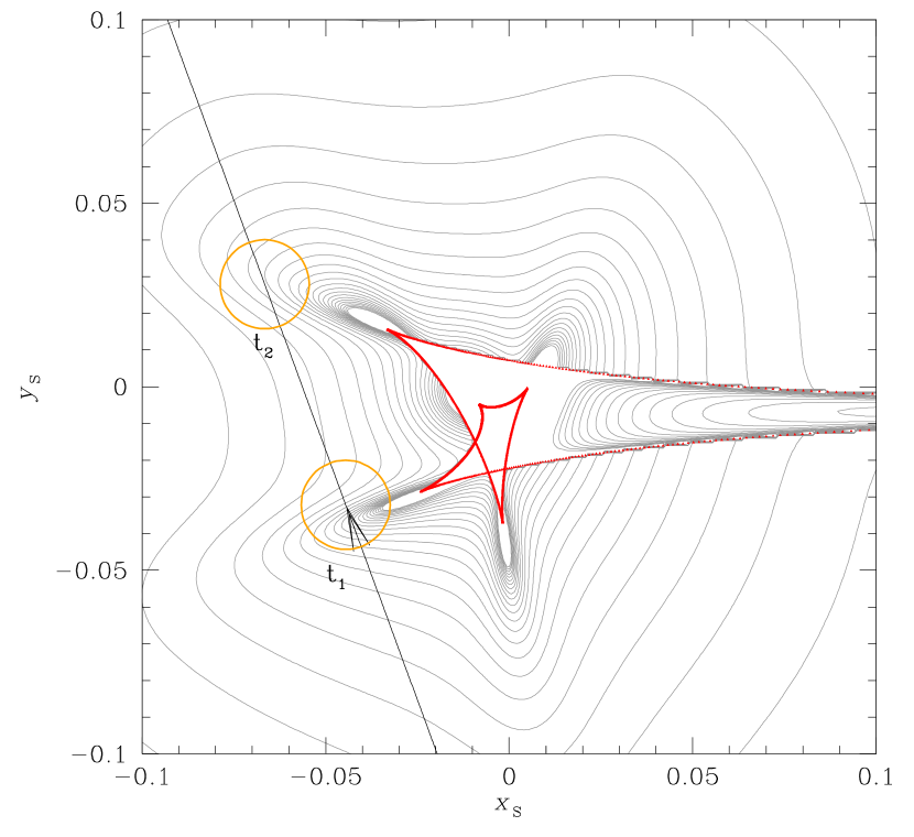
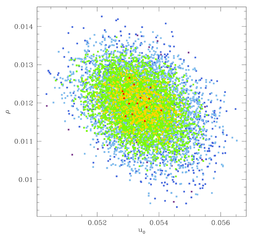
For the “multiple-planet (II)” solutions, the source does not cross the caustic, but finite-source effects are securely detected unlike the previous two sets of 3L1S solutions. To investigate the reason for this, we construct the magnification pattern around the central caustic. Figure 14 shows the constructed magnification contour map, in which the innermost contour is drawn at $A=50$ and the other contours are drawn at the descending magnifications with a step $\Delta A=2$ from the center toward outward. The line with an arrow represents the source trajectory and the two orange circles on the trajectory represent the source locations at the times of the first ($t_{1}$) and second ($t_{2}$) caustic approaches, respectively, and the size of the circle is scaled to the source size. We find that the magnification on the surface of the source varies substantially and this results in deviation of the light curve from the point-source light curve during the times around both bumps. From the deviation of the light curve, the normalized source radius is securely measured. Although there is some variation depending on the solution, the measured normalized source radius is $\rho\sim 0.012$. In Figure 15, we present the distribution of points in the MCMC chain on the $u_{0}$–$\rho$ plane for the best-fit “multiple-planet (II)” solution. Higher-order effects are not detected for the solution.

5.4. Comparison of Models

Because the overall features of the observed central perturbation are described by three sets of 3L1S solutions, we closely investigate the individual solutions. For this, we construct a cumulative distribution of $\Delta\chi^{2}=\chi^{2}_{\rm p-b}-\chi^{2}_{\rm m-p}$ for the data around the region of the anomaly. Here the subscripts “p-b” and “m-p” denote “planet-binary” and “multiple-planet” solutions, respectively. In Figure 16, we present the constructed cumulative $\Delta\chi^{2}$ distributions.

From the cumulative $\Delta\chi^{2}$ distributions, together with the residuals of the three solutions presented in Figure 10, we find that the “multiple-planet (II)” solution provides a better fit over the other two solutions. Compared to the “planet-binary” solution, the “multiple-planet (II)” solution better explains the rising part of the light curve in the region of the anomaly at ${\rm HJD}^{\prime}\sim 8285.2$, resulting in a better fit by $\Delta\chi^{2}=107.7$ over the “planet-binary” solution. The “planet-binary” solution is additionally disfavored by Occam’s razor because the major features occur only during the gap in the data. Compared to the “multiple-planet (I)” solution, the “multiple-planet (II)” solution better describes the light curve in the region $8282.0\lesssim{\rm HJD}^{\prime}\lesssim 8284.1$, resulting in a better fit by $\Delta\chi^{2}=65.9$. We note that according to the “multiple-planet (I)” solution, the source approached a cusp of the caustic induced by $M_{3}$ at around $t^{\prime}\sim 8283.0$, producing a weak bump. However, no such a bump is expected according to the “multiple-planet (II)” solution, and this makes the solution better fit the data over the “multiple-planet (I)” solution. Considering the better description of the detailed structures of the lensing light curve over the other models, we conclude that the “multiple-planet (II)” solution provides the most plausible model of the observed data.

Figure 16.— Cumulative distribution of $\Delta\chi^{2}=\chi^{2}_{\rm p-b}-\chi^{2}_{\rm m-p}$ between the planet-binary and “multiple-planet” 3L1S solutions for the data in the regions of the anomaly. Here the subscripts “p-b” and “m-p” denote planet-binary and “multiple-planet” solutions, respectively. The light curve in the upper panel is presented to show the regions of $\chi^{2}$ difference.

6. Source Star

Characterizing a source star in microlensing is important in order to estimate the angular Einstein radius, $\theta_{\rm E}$, that is related to the angular source radius $\theta_{*}$ by

$$\theta_{\rm E}={\theta_{*}\over\rho}.$$ (2)

For OGLE-2018-BLG-1011, the normalized source radius is securely measured despite that the source does not cross the caustic. Then, one needs to estimate the angular source radius to estimate the angular Einstein radius.

Figure 17.— Position of the source with respect to the centroid of red giant clump (RGC) in the instrumental color-magnitude diagram of stars around the source. Also marked is the position of the blend.

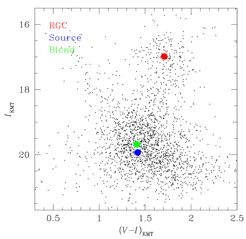
For the estimation of the angular source radius, we first estimate the de-reddened color $(V-I)_{\rm S,0}$ and brightness $I_{\rm S,0}$ of the source star. For this estimation, we use the Yoo et al. (2004) method, in which the color and magnitude are calibrated using the centroid of the red giant clump (RGC) in the color-magnitude diagram (CMD) as a reference. In Figure 17, we present the location of the source in the CMD of stars within $\sim 20^{\prime}$ around the source star. The CMD is constructed based on the pyDIA photometry of the KMTC $I$- and $V$-band data sets. The instrumental color and brightness of the source are $(V-I,I)_{\rm S}=(1.42\pm 0.01,19.93\pm 0.01)$. The offsets in color and magnitude of the source with respect to the RGC centroid, which is located at $(V-I,I)_{\rm RGC}=(1.71,16.99)$, are $\Delta(V-I,I)_{\rm S}=(-0.29,2.95)$. With the known de-reddened values of the RGC centroid of $(V-I,I)_{\rm RGC,0}=(1.06,14.38)$ (Bensby et al., 2011; Nataf et al., 2013), then the de-reddened color and brightness of the source star are estimated as $(V-I,I)_{\rm S,0}=(V-I,I)_{\rm S}+\Delta(V-I,I)_{\rm S}=(0.77\pm 0.01,17.33\pm 0.01)$. These values indicate that the source is a late G-type turn-off star. In Figure 17, we also mark the position of the blend in the CMD. It is found that the blend has a color and a brightness that are similar to those of the source. The brightness of the blend is $I_{\rm b}=19.04\pm 0.01$ as measured in the OGLE photometry system, which is approximately calibrated.

Table 7Source, blend, Einstein radius, and proper motion

Quantity	Value
$(V-I)_{0}$	$0.77\pm 0.01$
$I_{0}$	$17.33\pm 0.01$
$I_{\rm b}$	$19.04\pm 0.01$
$\theta_{*}$ ($\mu$as)	$1.98\pm 0.08$
$\theta_{\rm E}$ (mas)	$0.09\pm 0.01$
$\mu$ (mas yr-1)	$2.81\pm 0.22$

Note. — The value $I_{\rm b}$ presents the $I$-band magnitude of the blend.

With the known de-reddened color and brightness, the angular source radius is estimated first by converting the $V-I$ color into the $V-K$ color using the color-color relation (Bessell & Brett, 1988) and second using the $(V-K)/\theta_{*}$ relation (Kervella et al., 2004). This procedure yields the angular source radius of

$$\theta_{*}=1.98\pm 0.08~{}\mu{\rm as}.$$ (3)

We note that two major factors affect the precision of the estimated angular source radius. The first is the uncertainty of the de-reddened color, $\sim 0.05$ mag, and the other is the uncertainty in the position of RGC, $\sim 0.1$ mag. The uncertainty of $\theta_{*}$ is estimated by considering the combined uncertainty, which is $\sim 7\%$, of these two factors (Gould, 2014a). With the measured $\theta_{*}$ together with $\rho$, the angular Einstein radius is estimated as

$$\theta_{\rm E}={\theta_{*}\over\rho}=0.09\pm 0.01~{}{\rm mas}.$$ (4)

With the angular Einstein radius combined with the event timescale, the relative lens-source proper motion is estimated as

$$\mu={\theta_{\rm E}\over t_{\rm E}}=2.81\pm 0.22~{}{\rm mas}.$$ (5)

In Table 7, we summarize the colors and magnitudes of the source and blend and the estimated angular source radius, Einstein radius, and the relative lens-source proper motion.

Figure 18.— The distributions of the lens mass (upper panel) and distance (lower panel) estimated by Bayesian analysis. The solid vertical line for each distribution indicates the median value, and the two dotted vertical lines represent the $1\sigma$ range of the estimated value, i.e., 16% and 84% of the distribution.

For an independent constraint on the source star distance, we check the source information in the list of Gaia data release 2 (Gaia DR2: Gaia Collaboration, 2018). However, there is no information of the absolute parallax and proper motion of the source because the source, with a $G$-band magnitude of $G=19.76$, is fainter than the Gaia limit of $G\sim 18$. As a result, it is difficult to constraint the source distance from the Gaia data.

7. Physical Parameters

For the unique determination of the mass, $M$, and distance to the lens, $D_{\rm L}$, one needs to measure both the angular Einstein radius $\theta_{\rm E}$ and the microlens parallax $\pi_{\rm E}$, which are related to $M$ and $D_{\rm L}$ by the relations

$$M={\theta_{\rm E}\over\kappa\pi_{\rm E}};\qquad D_{\rm L}={{\rm au}\over\pi_{\rm E}\theta_{\rm E}+\pi_{\rm S}},$$ (6)

where $\kappa=4G/(c^{2}{\rm au})$, $\pi_{\rm S}={\rm au}/D_{\rm S}$, and $D_{\rm S}$ is the source distance, which is $\sim 8$ kpc for a source star located in the bulge. For OGLE-2018-BLG-1011, the angular Einstein radius is measured, but the microlens parallax is not measured. We, therefore, estimate the physical lens parameters by conducting Bayesian analysis with the constraints of the measured $t_{\rm E}$ and $\theta_{\rm E}$.

A microlensing Bayesian analysis requires prior models of the lens mass function and the physical and dynamical distributions of the Galaxy. We adopt the mass function of Chabrier (2003) for stars and that of Gould (2000) for stellar remnants. For the physical and dynamical distributions, we adopt Han & Gould (2003) and Han & Gould (1995) models, respectively. For more details of these models, see section 5 of Han et al. (2018). Based on these priors, we conduct a Monte Carlo simulation and produce $2\times 10^{6}$ microlensing events. We then construct the distributions $M$ and $D_{\rm L}$ for events that have timescales and angular Einstein radii within the ranges of the measured $t_{\rm E}$ and $\theta_{\rm E}$. We estimate $M$ and $D_{\rm L}$ as the median values of the distributions and their lower and upper limits are estimated as the 16% and 84% of the distributions, respectively.

In the Bayesian analysis, we also impose the constraint of the lens brightness so that the lens cannot be brighter than the measured blend brightness of $I_{\rm b}\sim 19.0$. The lens brightness is computed based on the mass, distance, and extinction. We assume that the extinction linearly increases with distance until it becomes $A_{I}\sim 1.68$ at $D_{\rm S}$, which is the measured value of the extinction toward the field. We find that this constraint has little effect on the lens mass and distance distributions. This is because lenses, in most cases, are much fainter than the blend. For the same reason, the result would not change with the choice of different extinction model along the line of sight.

Table 8Physical lens parameters

Parameter	Value
$M_{1}$ ($M_{\odot}$)	$0.18^{+0.33}_{-0.10}$
$M_{2}$ ($M_{\rm J}$)	$1.8^{+3.4}_{-1.1}$
$M_{3}$ ($M_{\rm J}$)	$2.8^{+5.1}_{-1.7}$
$D_{\rm L}$ (kpc)	$7.1^{+1.1}_{-1.5}$
$a_{\perp,2}$ (au)	$1.8^{+2.1}_{-1.5}$ ($0.8^{+0.9}_{-0.6}$)
$a_{\perp,3}$ (au)	$0.8^{+0.9}_{-0.6}$

Note. — The $a_{\perp,2}$ value in the parenthesis is for the solution with $s_{2}>1.0$.

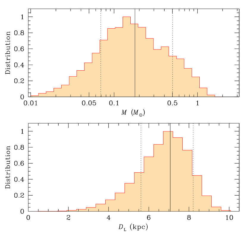
In Figure 18, we present the distributions of the lens mass and the distance obtained from the Bayesian analysis. In Table 8, we list the estimated values of the individual lens components, $M_{1}$, $M_{2}$, and $M_{3}$, the distance to the lens, $D_{\rm L}$, and the projected separations of the planets from the host, $a_{\perp,2}$ and $a_{\perp,3}$. It is found that the lens is a multiple-planet system composed of two giant planets with masses

$$M_{2}=1.8^{+3.4}_{-1.1}~{}M_{\rm J}$$ (7)

and

$$M_{3}=2.8^{+5.1}_{-1.7}~{}M_{\rm J}$$ (8)

around a host star with a mass

$$M_{1}=0.18^{+0.33}_{-0.10}~{}M_{\odot}.$$ (9)

The distance to the lens is estimated as

$$D_{\rm L}=7.1^{+1.1}_{-1.5}~{}{\rm kpc}.$$ (10)

The estimated distance indicates that the lens is the farthest system among the known multiplanetary systems. We note that the previous multiplanetary system with the farthest distance is OGLE-2012-BLG-0026L that is located at $\sim 4.0\pm 0.3$ kpc away (Han et al., 2013; Beaulieu et al., 2016). The projected separations of the planets from the host are

$$a_{\perp,2}=1.8^{+2.1}_{-1.5}~{}\left(0.8^{+0.9}_{-0.6}\right)~{}{\rm au}$$ (11)

and

$$a_{\perp,3}=0.8^{+0.9}_{-0.6}~{}{\rm au}.$$ (12)

We note that the value of $a_{\perp,2}$ in the parenthesis of equation (11) is for the solution with $s_{2}<1.0$. The snow line of the planetary system is $a_{\rm sl}\sim 2.7~{}{\rm au}~{}(M/M_{\odot})\sim 0.5~{}{\rm au}$, and thus both planets are located beyond the snow line of the host similar to the other cases of the multiplanetary systems found by microlensing.

8. Discussion and Conclusion

We investigated the microlensing event OGLE-2018-BLG-1011, for which the light curve exhibited an anomaly around the peak. We found that it was not possible to reasonably explain the anomaly with the binary-lens or binary-source interpretations and its description required the introduction of an additional lens component. The 3L1S modeling resulted in three sets of solutions, in which one set of solutions indicated that the lens was a planetary system in a binary, while the other two sets of solutions implied that the lens was a multiplanetary system. By investigating the fits of the individual models to the detailed structure of the lensing light curve, we found that the multiple-planet solutions with planet-to-host mass ratios $\sim 9.5\times 10^{-3}$ and $15\times 10^{-3}$ were favored over the other solutions. From the Bayesian analysis for the best-fit solution, it was found that the lens is a multiple planetary system composed of giant planets with masses $\sim 1.8~{}M_{\rm J}$ and $\sim 2.8~{}M_{\rm J}$ orbiting a bulge star with a mass $\sim 0.18~{}M_{\odot}$ located at a distance of $\sim 7.1~{}{\rm kpc}$. The projected separations of the planets from the host were $a_{\perp,2}\sim 1.8~{}{\rm au}$ (or $\sim 0.8~{}{\rm au}$) and $a_{\perp,3}\sim 0.8~{}{\rm au}$, where the values of $a_{\perp,2}$ denoted with and without parentheses were the separations corresponding to the two degenerate solutions with close and wide separations. Therefore, both planets were located beyond the snow line of the host similar to the other four multiplanetary systems previously found by microlensing.

References

- Alard & Lupton (1998) Alard, C., & Lupton, R. H. 1998, ApJ, 503, 325
- Albrow (2017) Albrow, M. 2017, MichaelDAlbrow/pyDIA: Initial Release on Github, doi: 10.5281/zenodo.268049
- Albrow et al. (2000) Albrow, M. D., Beaulieu, J.-P., Caldwell, J. A. R., et al. 2000, ApJ, 534, 894
- Beaulieu et al. (2016) Beaulieu, J.-P., Bennett, D. P., Batista, V., et al. 2016, ApJ, 824, 83
- Bennett et al. (1999) Bennett, D. P., Rhie, S. H., Becker, A. C., et al. 1999, Nature, 402, 57
- Bennett et al. (2010) Bennett, D. P., Rhie, S. H., Nikolaev, S., et al. 2010, ApJ, 713, 837
- Bennett et al. (2016) Bennett, D. P., Rhie, S. H., Udalski, A., et al. 2016, AJ, 152, 125
- Bensby et al. (2011) Bensby, T., Adén, D., Meléndez, J., et al. 2011, PASP, 533, 134
- Bessell & Brett (1988) Bessell, M. S., & Brett, J. M. 1988, PASP, 100, 1134
- Bond et al. (2001) Bond, I. A., Abe, F., Dodd, R. J., et al. 2001, MNRAS, 327, 868
- Bozza et al. (2016) Bozza, V., Shvartzvald, Y., Udalski, A., et al. 2016, ApJ, 820, 79
- Breger et al. (1993) Breger, M., Stich, J., Garrido, R., et al. 1993, A&A, 271, 482
- Chabrier (2003) Chabrier, G. 2003, ApJ, 586, L133
- Choi et al. (2012) Choi, J.-Y., Shin, I.-G., Han, C., et al. 2012, ApJ, 756, 48
- Cleeves (2016) Cleeves, L. I. 2016, ApJ, 816, L21
- Daněk & Heyrovský (2015) Daněk, K., & Heyrovský, D. 2015, ApJ, 806, 99
- Daněk & Heyrovský (2019) Daněk, K., & Heyrovský, D. 2019, arXiv:1901.08610
- Dominik (1998) Dominik, M. 1998, A&A, 329, 36
- Dominik (1999) Dominik, M. 1999, A&A, 349, 108
- Dominik et al. (2019) Dominik, M., Bachelet, E., Bozza, V., et al. 2019, MNRAS, 484, 5608
- Gaia Collaboration (2018) Gaia Collaboration, et al. 2018, A&A, 616, 1
- Gaudi (1998) Gaudi, B. S. 1998, ApJ, 506, 533
- Gaudi et al. (1998) Gaudi, B. S., Naber, R. M., & Sackett, P. D. 1998, ApJ, .502, L33
- Gaudi et al. (2008) Gaudi, B. S., Bennett, D. P., Udalski, A., et al. 2008, Science, 319, 927
- Gaudi & Han (2004) Gaudi, B. S., & Han, C. 2004, ApJ, 611, 528
- Gould (1992) Gould, A. 1992, ApJ, 392, 442
- Gould (2000) Gould, A. 2000, ApJ, 535, 928
- Gould (2014) Gould, A. 2014, JKAS, 47, 215
- Gould et al. (2010) Gould, A., Dong, S., Gaudi, B. S., et al. 2010, ApJ, 720, 1073
- Gould (2014a) Gould, A. 2014a, JKAS, 47, 153
- Gould et al. (2014b) Gould, A., Udalski, A., Shin, I.-G., et al. 2014b, Science, 345, 46
- Griest & Safazadeh (1998) Griest, K., & Safazadeh, N. 1998, ApJ, 500, 37
- Han (2005) Han, C. 2005, ApJ, 629, 1102
- Han et al. (2016) Han, C., Bennett, D. P., Udalski, A., & Jung, Y. K. 2016, ApJ, 825, 8
- Han et al. (2018) Han, C., Bond, I. A., Gould, A., et al. 2018, AJ, 156, 226
- Han & Gaudi (2008) Han, C., & Gaudi, B. S. 2008, ApJ, 689, 53
- Han & Gould (1995) Han, C., & Gould, A. 1995, ApJ, 447, 53
- Han & Gould (2003) Han, C., & Gould, A. 2003, ApJ, 592, 172
- Han et al. (2013) Han, C., Udalski, A., Choi, J.-Y., et al. 2013, ApJ, 762, L28
- Han et al. (2017) Han, C., Udalski, A., Gould, A., et al. 2017, AJ, 154, 223
- Hwang et al. (2013) Hwang, K.-H., Choi, J.-Y., Bond, I. A., et al. 2013, ApJ, 778, 55
- Ioka et al. (1999) Ioka, K., Nishi, R., & Kan-Ya, Y. 1999, PThPh, 102, 98
- Jung et al. (2013) Jung, Y. K., Han, C., Gould, A., & Maoz, D. 2013, ApJ, 768, L7
- Jung et al. (2017) Jung, Y. K., Udalski, A., Yee, J. C., et al. 2017, AJ, 153, 129
- Kervella et al. (2004) Kervella, P., Thévenin, F., Di Folco, E., & Ségransan, D. 2004, A&A, 426, 29
- Kim et al. (2018) Kim, D.-J., Kim, H.-W., Hwang, K.-H. et al. 2018, AJ, 155, 76
- Kim et al. (2016) Kim, S.-L., Lee, C.-U., Park, B.-G., et al. 2016, JKAS, 49, 37
- Lenz & Breger (2005) Lenz, P., & Breger, M. 2005, Communications in Asteroseismology, 146, 53
- Lin et al. (1996) Lin, D. N. C., Bodenheimer, P., & Richardson, D. C. 1996, Nature, 380, 606
- Madsen & Zhu (2019) Madsen, S., & Zhu, W. 2019, arXiv:1901.04495
- Mizuno (1980) Mizuno, H. 1980, Progress of Theoretical Physics, 64, 544-557
- Murray et al. (1998) Murray, N., Hansen, B., Holman, M., & Tremaine, S. 1998, Science, 279, 69
- Nataf et al. (2013) Nataf, D. M., Gould, A., Fouqué, P., et al. 2013, ApJ, 769, 88
- Park et al. (2014) Park, H., Han, C., Gould, A., et al. 2014, ApJ, 787, 71
- Poleski (2014) Poleski, R., Skowron, J., Udalski, A., et al. 2014, ApJ, 795, 42
- Pollack et al. (1996) Pollack, J. B., Hubickyj, O., Bodenheimer, P., Lissauer, J. J., Podolak, M., & Greenzweig, Y. 1996, Icarus, 124, 62
- Ryu et al. (2019) Ryu, Y.-H., Udalski, A., Yee, J. C., et al. 2019, arXiv:1905.08148
- Shin et al. (2019) Shin, I.-G., Yee, J. C., Gould, A., et al. 2019, arXiv:1902.10945
- Shvartzvald et al. (2017) Shvartzvald, Y., Bryden, G., Gould, A., Henderson, C. B., Howell, S. B., & Beichman, C. 2017, AJ, 153, 61
- Stevenson (1982) Stevenson, D. J. 1982, Planetary and Space Science, 30, 755
- Sumi et al. (2003) Sumi, T., Abe, F., Bond, I. A., et al. 2003, ApJ, 591, 20
- Suzuki et al. (2016) Suzuki, D., Bennett, D. P., Sumi, T., et al. 2016, ApJ, 833, 145
- Suzuki et al. (2018) Suzuki, D., Bennett, D. P., Udalski, A., et al. 2018, AJ, 155, 263
- Udalski et al. (2015a) Udalski, A., Jung, Y. K., Han, C., et al. 2015a, ApJ, 812, 47
- Udalski et al. (2015b) Udalski, A., Szymański, M. K., & Szymański, G. 2015b, Acta Astron., 65, 1
- Ward (1997) Ward, W. R. 1997, Icarus, 126, 261
- Woźniak (2000) Woźniak, P. R. 2000, Acta Astron., 50, 42
- Yee et al. (2012) Yee, J. C., Shvartzvald, Y., Gal-Yam, A., et al. 2012, ApJ, 755, 102
- Yoo et al. (2004) Yoo, J., DePoy, D. L., Gal-Yam, A., et al. 2004, ApJ, 603, 139
- Zang et al. (2018) Zang, W., Penny, M., Zhu, W., et al. 2018, PASP, 130, 104401