Constraining the inner density slope of massive galaxy clusters

Abstract

We determine the inner density profiles of massive galaxy clusters (M${}_{\rm 200}>5\times 10^{14}$ ${\rm M}_{\odot}$) in the Cluster-EAGLE (C-EAGLE) hydrodynamic simulations, and investigate whether the dark matter density profiles can be correctly estimated from a combination of mock stellar kinematical and gravitational lensing data. From fitting mock stellar kinematics and lensing data generated from the simulations, we find that the inner density slopes of both the total and the dark matter mass distributions can be inferred reasonably well. We compare the density slopes of C-EAGLE clusters with those derived by Newman et al. for 7 massive galaxy clusters in the local Universe. We find that the asymptotic best-fit inner slopes of “generalized” NFW (gNFW) profiles, $\gamma_{\rm gNFW}$, of the dark matter haloes of the C-EAGLE clusters are significantly steeper than those inferred by Newman et al. However, the mean mass-weighted dark matter density slopes of the simulated clusters are in good agreement with the Newman et al. estimates. We also find that the estimate of $\gamma_{\rm gNFW}$ is very sensitive to the constraints from weak lensing measurements in the outer parts of the cluster and a bias can lead to an underestimate of $\gamma_{\rm gNFW}$.

1 Introduction

In the $\Lambda$CDM cosmological model cold dark matter dominates the matter budget of the Universe, and much of it clusters into dark matter halos. Gas condenses at the centres of these haloes, forming stars and giving birth to galaxies (White & Rees, 1978; White & Frenk, 1991). Measuring the distributions of dark and baryonic matter at the centres of haloes provides a key test of $\Lambda$CDM and theories of galaxy formation.

Over the past three decades, the evolution of pure cold dark matter has been calculated with great precision by means of N-body simulations (Davis et al., 1985; Navarro et al., 1996b, 1997; Jenkins et al., 2001; Diemand et al., 2007; Springel et al., 2008; Gao et al., 2011) (for a review see Frenk & White, 2012). In particular, Navarro et al. (1996b, 1997, hereafter NFW) have shown that dark matter haloes have a universal, self-similar, spherically averaged mass profile with asymptotic behaviour, $\rho(r)\propto r^{-1}$, at the centre, and $\rho(r)\propto r^{-3}$ at large radii.

In reality, in a bright galaxy baryonic matter dominates the mass budget at the centre of the halo (Schaller et al., 2015a). Furthermore, the galaxy formation process may modify the central halo density itself. The effects of these baryonic processes are complex and even their sign is unclear: while baryon condensation and contraction may sharpen the density profile (Blumenthal et al., 1986; Gnedin et al., 2004; Gustafsson et al., 2006; Duffy et al., 2010; Schaller et al., 2015a; Peirani et al., 2017), rapid expulsion of gas due to feedback process may flatten it, at least in faint galaxies (e.g. Navarro et al., 1996a; Dehnen, 2005; Read & Gilmore, 2005; Mashchenko et al., 2006; Pontzen & Governato, 2012). The competition between these processes is best followed with hydrodynamical simulations, but even then discrepancies persist. For example, Gnedin et al. (2011) and Schaller et al. (2015a, b) show that the net effect of baryonic processes in large galaxies in the field and in clusters is to preserve the asymptotic dark matter density profile, $\rho(r)\propto-1$, but Martizzi et al. (2013) find that cores may be generated by AGN feedback in extreme cases.

Observationally, the inner density slopes of bright galaxies are best constrained by combining stellar dynamics data for the central galaxy with gravitational lensing data at large radii (e.g. Treu & Koopmans, 2002, 2004; Auger et al., 2010; Sonnenfeld et al., 2015; Newman et al., 2013a; Newman et al., 2013b, 2015; Shu et al., 2015). In this way the total density profile of a galaxy can be measured, from several kiloparsecs to tens of kiloparsecs from the centre. The total mass-averaged density slope, $\bar{\gamma}$, within the effective radius of early type galaxies is found to be around -2 in galaxy and group scale systems, but may drop gradually to -1.2 in massive clusters (Treu & Koopmans, 2004; Auger et al., 2010; Newman et al., 2015; Li et al., 2019). The dark matter halo profile is not directly measurable and can only be inferred by assuming a model to subtract the contribution from the stellar component. Recent measurements have concluded that while the halo density profile in groups is consistent with the NFW form (Newman et al., 2015; Smith et al., 2017), some clusters the inner slope is around -0.5, significantly shallower than the NFW prediction (Sand et al., 2004; Sand et al., 2008; Newman et al., 2013b; Del Popolo et al., 2019), and in contradiction with cosmological simulation results.

There are several possible interpretations for this discrepancy. The simulations may lack the correct physics, or treat baryonic processes improperly (Laporte et al., 2012; Laporte & White, 2015), or it may be that the dark matter is not cold but perhaps made up of self-interacting particles (e.g. Spergel & Steinhardt, 2000; Vogelsberger et al., 2012; Rocha et al., 2013; Kaplinghat et al., 2016; Robertson et al., 2017a, b). An alternative explanation is that systematic effects in the analysis of the observational data have been underestimated.

There are several potential sources of systematic uncertainties when subtracting the stellar component in order to infer the inner slope of the dark matter component. For example, the shape of the stellar density profile is usually inferred from the light profile either assuming a constant mass-to-light ratio or a stellar population synthesis model (e.g. Cappellari, 2008; Newman et al., 2013a; Newman et al., 2015). A systematic overestimation of the mass-to-light ratio could relieve the tension between observations and theory (Schaller et al., 2015b). In addition, simplistic assumptions about the symmetry of the system or the anisotropy of the velocity distribution may also bias the inference of the inner dark matter profile (e.g. Meneghetti et al., 2007; Li et al., 2016). Recently, Sartoris et al. (2020) have estimated a value of -0.99 for the dark matter density slope at the centre of Abell S1063 – in excellent agreement with $\Lambda$CDM predictions – from analysis of a large sample of stars in the central galaxy with spectroscopic data and a model allowing for variable velocity dispersion anisotropy.

In this work we assess dark matter density reconstruction methods in galaxy clusters that combine stellar dynamics with gravitational lensing. We construct mock data using the C-EAGLE simulations, a set of high resolution zoom-in hydrodynamical simulations of massive clusters (Barnes et al., 2017; Bahé et al., 2017). We then perform a combined analysis of stellar kinematics and gravitational lensing on the mock data and explore the accuracy of the recovered dark matter density profiles.

The structure of the paper is as follows. In Section 2 we describe our mock data and in Section 3 our models, and the method used to infer model parameters. In Section 4 we present the recovery of dark matter profiles and study the model dependence on galaxy shape and velocity anisotropy. We summarize and discuss our results in Section 5.

2 Mock data

2.1 The C-EAGLE simulations

We create mock observations using the C-EAGLE simulations (Bahé et al., 2017; Barnes et al., 2017). This set of cosmological hydrodynamical simulations consists of 30 zoom-in resimulated massive galaxy clusters that were selected from a larger volume dark matter-only simulation according to a criterion based on halo mass and isolation (Bahé et al., 2017). The C-EAGLE simulations employ the state-of-the-art EAGLE galaxy formation model and simulation code (Schaye et al., 2015; Crain et al., 2015). This code is based on a modified version of the gadget-3 smooth particle hydrodynamics (SPH) code last described in Springel (2005), which include radiative cooling, star formation, stellar and black hole feedback, etc. The parameters of the subgrid models used for EAGLE were calibrated so as to reproduce a small subset of data of the z=0 field galaxy population(Schaye et al., 2015; Crain et al., 2015). C-EAGLE made use of the AGNdT9 model which gives a better match than the reference EAGLE model to the X-ray luminosities and gas fractions of low-mass galaxy groups (Schaye et al., 2015). C-EAGLE adopted the same $\Lambda$CDM cosmological parameters as EAGLE: H${}_{0}=67.77$km s^-1 Mpc^-1, $\Omega_{\Lambda}=0.693$, $\Omega_{\rm M}=0.307$ and $\Omega_{\rm b}=0.04825$. The mass resolution of C-EAGLE is the same as in EAGLE: $1.8\times 10^{6}\,\mathrm{M}_{\odot}$ initially for gas particles and $9.7\times 10^{6}\,\mathrm{M}_{\odot}$ for dark matter particles. The Plummer gravitational softening length of the high-resolution region was set to 2.66 comoving $\mathrm{kpc}$ for $z>2.8$, and then kept fixed at $0.70$ physical $\mathrm{kpc}$ for $z<2.8$. The minimum smoothing length of the SPH kernel was set to a tenth of the gravitational softening scale.

In this paper we are interested in massive clusters comparable to those in the sample of Newman et al. (2013a); Newman et al. (2013b) and so we focus on clusters whose mass falls in the range $4.0\times 10^{14}<M_{200}<2\times 10^{15}\,\mathrm{M}_{\odot}$ at $z=0$, where $M_{200}$ is the mass enclosed within a sphere of radius $r_{200}$ whose mean density is 200 times the critical density of the universe. Altogether our sample consists of 17 massive galaxy clusters, denoted by CE-12 to CE-28 in the C-EAGLE simulations (Barnes et al., 2017). While the clusters analyzed by Newman et al. (2013a); Newman et al. (2013b) have an average redshift of $z\sim$ 0.2, the simulation output we analyze is at $z=0$. However, we have checked that our conclusions are unaffected by this choice. Further properties of our clusters may be found in the tables in the Appendix of Barnes et al. (2017); Bahé et al. (2017).

2.2 Photometric and kinematic data

We create photometric and kinematic mock data following a similar process to that described by Li et al. (2016). First, we define the central galaxy as the one lying closest to the centre of the potential of the cluster. Using the same method as Schaller et al. (2015c), we find that all our central galaxies are very close to the centre of the potential, with a mean offset of 0.2  kpc and a maximum of 0.8 kpc. Since the offset is comparable to the softening length of the simulations (0.70 kpc), the centres of the central galaxies are consistent with the centres of the potential. Next, we construct the surface stellar mass density map of the central galaxies in the C-EAGLE clusters by projecting the galaxy’s star particles onto the $x-y$ plane of the simulation volume on a grid of cellsize $0.5\times 0.5\,\mathrm{kpc}^{2}$.

To generate a brightness map we assume a constant $M^{*}/L$ ratio for each star particle. For comparison, we also generate a surface brightness map for each central galaxy by calculating the mass-weighted r-band brightness in each cell. The luminosities of individual star particles are derived following the method of Trayford et al. (2015).

We then calculate the mean and standard deviation of the line-of-sight velocities of stars in each cell. As Newman et al. (2013a), we obtain kinematic data in a long slit of width $3\,\mathrm{kpc}$ aligned with the major axis of the galaxy. The bins extend from the galactic centre to $21\,\mathrm{kpc}$, which is approximately $1.5$ effective radii ($R_{E}$) for the galaxies in our sample. We assume that the uncertainty in the measured velocity dispersion is $6$ percent in the inner four bins and $9$ percent in the outer three bins, similar to the values in Newman et al. (2013a). For the situation where a satellite happens to lie along the line-of-sight, we discard the affected bins.

In Fig. 1, we compare the line-of-sight velocity dispersion profiles for our sample of clusters with those from Newman et al. (2013a). The blue points are the velocity dispersions of the Newman et al. (2013a) clusters and the red points are those of our clusters. The vertical dotted line marks the softening length and the vertical dashed line is the 3D average Power et al. radius (Power et al., 2003), which is usually taken to define the region where the profiles are numerically converged. Here, we adopt the same threshold as Schaller et al. (2015a) to derive the Power et al. radius for our clusters. As we can see, most our clusters have higher line-of-sight velocity dispersions than the observed clusters. This is because at a given halo mass, the brightest cluster galaxies (BCGs) in C-EAGLE contain more stellar mass than observed BCGs by up to 0.6 dex (Bahé et al., 2017) and this results in a greater mass concentration and thus a larger velocity dispersion reflecting the deeper gravitational potential.

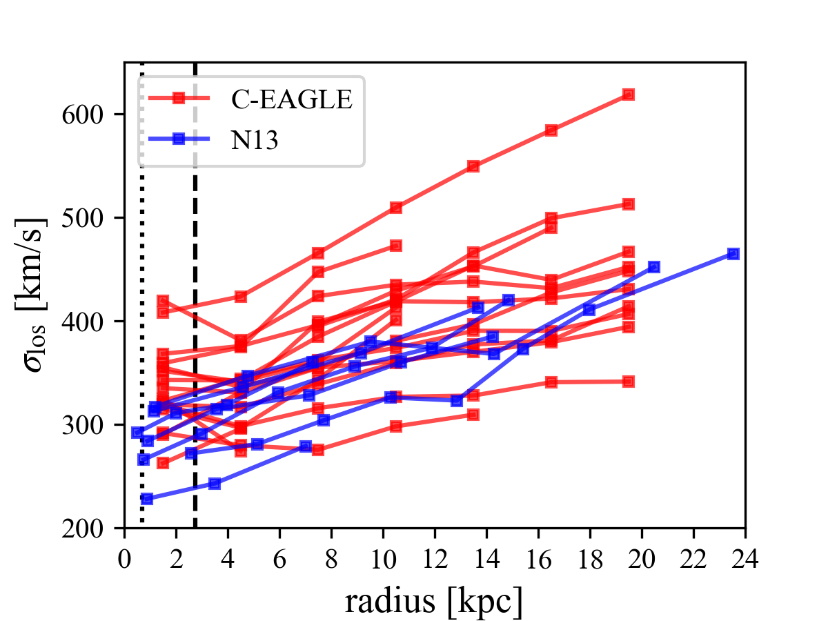
Figure 1: Line-of-sight velocity dispersion profiles. Red and blue lines represent profiles derived for our sample of BCGs and those from derived from the observed data in Newman et al. (2013a), respectively. The vertical dotted line marks the softening length and the vertical dashed line the 3D average Power et al. radius for our clusters.

2.3 Gravitational lensing mock data

We calculate the tangential shear of the clusters at ten equally spaced logarithmic bins in radius ranging from $100\,\mathrm{kpc}$ to $2000\,\mathrm{kpc}$, which is similar to the range covered by the data of Newman et al. (2013a); Newman et al. (2013b). Since the shear contributed by the correlation between different haloes is much smaller than the shear caused by the halo itself (Cacciato et al., 2009; Li et al., 2009), for simplicity, the lensing signal is calculated only from the mass distribution in the halo ignoring the contribution of the large-scale structure. The tangential shear, $\gamma_{t}$, at projected radius, $R$, can be written as,

$$\gamma_{t}(R)\Sigma_{\rm crit}=\Delta\Sigma(R)=M_{\rm surf}(R)/(\pi R^{2})-\Sigma(R),$$ (1)

where $M_{\rm surf}(R)$ is the mass, including dark matter, stars and gas, enclosed within projected radius, $R$; $\Sigma(R)$ is the surface density at $R$; and $\Sigma_{\rm crit}$ is the critical surface density, which is determined from the redshifts of the lens and the source. We assume that the error on the tangential shear is $40\%$, comparable to the average error in Fig. 5 of Newman et al. (2013a). In this work, we do not perturb the true value, so the centre points of our weak lensing “measurements” are not biased.

Strong lensing is also important in constraining the mass model of the clusters. The observations usually consist of multiple arcs produced by different background galaxies at different redshifts and those arcs can be very sensitive to the local surface density. The strong lensing constraint in Newman et al. (2013a) comes from measurements of the positions of multiple images, whose uncertainty is taken to be 0.5  arcsecs. Here, to simplify our modelling, we approximate the strong lensing constraint as an aperture mass. The average Einstein radius, $R_{\rm Ein}$, of the Newman et al clusters is $\sim$ 10 arcsecs; thus we assume that the total projected mass within $R_{\rm Ein}$ ($\sim 39$ kpc at $z=0.2$) can be measured to a precision of $5\%$.

3 Models

We use two approaches to model the stellar kinematics of the central galaxies in the C-EAGLE clusters:

1. the spherically symmetric Jeans model (sJ) (Binney & Tremaine, 2008; Cappellari, 2008)

2. the Jeans anisotropic model (JAM) (Emsellem et al., 1994; Cappellari, 2002, 2008).

Since Newman et al. (2013a); Newman et al. (2013b) mainly used sJ, when comparing our results with observations, we will mostly rely on this model as well. However, for an interesting theoretical test, we also combine JAM with the lensing analysis to investigate if it results in significant differences.

3.1 sJ Model

For the spherically symmetric case, the Jeans equation gives the relation between the line-of-sight velocity dispersion, $\sigma_{\rm los}$, and the mass distribution, $M_{\rm tot}(r)$, as:

$$\sigma_{\rm los}(R)=\frac{2G}{\Sigma_{*}(R)}\int_{R}^{\infty}\frac{\rho_{*}(r)M_{\rm tot}(r)F(r)}{r^{2}}dr\>,$$ (2)

where $\Sigma_{*}$ and $\rho_{*}$ are the surface density and 3D density of the stars, respectively, $M_{\rm tot}(r)$ is the total mass enclosed within 3D radius $r$ and, in the isotropic case, $F(r)=\sqrt{r^{2}-R^{2}}$.

Following Newman et al. (2013a), we use a 3-parameter dPIE model (Elíasdóttir et al., 2007) to describe the 3D density profile of the stellar component, where,

$$\rho_{\rm dPIE}(r)=\frac{\rho_{0}}{(1+r^{2}/a^{2})(1+r^{2}/s^{2})}\>;$$ (3)

the core radius, $a$, the scale radius, $s$ ($s>a$), and the central density, $\rho_{0}$, are free parameters. The surface density profile of the stellar component can be analytically written as:

$$\Sigma_{\rm dPIE}(R)=\rho_{0}\frac{\pi a^{2}s^{2}}{s^{2}-a^{2}}\left(\frac{1}{\sqrt{a^{2}+R^{2}}}-\frac{1}{\sqrt{s^{2}+R^{2}}}\right)\>.$$ (4)

We fix the profile parameters, $a$ and $s$, by fitting the dPIE model to the mass surface density profile of the central galaxy. Only the normalization of the density profile is allowed to vary during the dynamical modeling process.

The mass distribution of the dark matter halo follows a gNFW profile:

$$\rho_{\rm gNFW}(r)=\rho_{s}\left(\frac{r}{r_{s}}\right)^{-\gamma_{\rm gNFW}}\left(\frac{1}{2}+\frac{1}{2}\frac{r}{r_{s}}\right)^{\gamma_{\rm gNFW}-3}\>,$$ (5)

where $\rho_{s}$ is the characteristic density and $\gamma_{\rm gNFW}$ gives the inner asymptotic density slope of the halo. For the NFW profile, $\gamma_{\rm gNFW}=1$.

For the spherical Jeans model we therefore have the following free parameters:

1. the stellar mass-to-light ratio: $M^{*}/L$;

2. the three parameters that describe the dark matter halo density profile: $\rho_{\rm s}$, $r_{s}$ and $\gamma_{\rm gNFW}$.

3.2 The JAM method

For many galaxies in the real Universe, the assumption of spherical symmetry for the distributions of mass and velocity dispersion are not valid. In practice, assuming an axisymmetric mass distribution often provides a better solution to galactic dynamical modeling.

For a steady-state axisymmetric mass distribution, the Jeans equations in cylindrical coordinates, $(R,z,\phi)$, can be written as:

$$\frac{n\overline{v_{R}^{2}}-n\overline{v_{\phi}^{2}}}{R}+\frac{\partial(n\overline{v_{R}^{2}})}{\partial R}+\frac{\partial(n\overline{v_{R}v_{z}})}{\partial z} = -n\frac{\partial\Phi_{\rm tot}}{\partial R},$$ (6)

$$\frac{n\overline{v_{R}v_{z}}}{R}+\frac{\partial(n\overline{v_{z}^{2}})}{\partial z}+\frac{\partial(n\overline{v_{R}v_{z}})}{\partial R} = -n\frac{\partial\Phi_{\rm tot}}{\partial z},$$ (7)

where the $v$s denote the three components of velocity,

$$n\overline{v_{k}v_{j}}\equiv\int v_{k}v_{j}f\;\mathrm{d}^{3}\mathbf{v},$$ (8)

$f$ is the distribution function of the stars, $\Phi_{\rm tot}$ the gravitational potential, and $n$ is the luminosity density.

In this work, we adopt the numerical Jeans-Anisotropic-Modeling routine of Cappellari (2008) with the multi-Gaussian Expansion (MGE) technique (Emsellem et al., 1994; Cappellari, 2002), which is widely used in galactic dynamical modeling (e.g. Cappellari, 2008; Cappellari et al., 2011; Newman et al., 2015; Li et al., 2016, 2017)

To determine a unique solution, the JAM routines make two assumptions (Cappellari, 2008):

1. the velocity dispersion ellipsoid is aligned with the cylindrical coordinate system ($\overline{v_{R}v_{z}}=0$),

2. the anisotropy in the meridional plane is constant, i.e. $\overline{v_{R}^{2}}=b\overline{v_{z}^{2}}$, where $b$ is related to $\beta_{z}$, the anisotropy parameter in the $z$ direction, defined as

   $$\beta_{z}\equiv 1-\frac{\overline{v_{z}^{2}}}{\overline{v_{R}^{2}}}\equiv 1-\frac{1}{b}\,.$$ (9)

If we set the boundary condition, $n\overline{v_{z}^{2}}=0$ as $z\rightarrow\infty$, the solution of Jeans equations can be written as

$$n\overline{v_{z}^{2}}(R,z) = \int_{z}^{\infty}n\frac{\partial\Phi_{\rm tot}}{\partial z}{\mathrm{d}}z$$ (10)

$$n\overline{v_{\phi}^{2}}(R,z) = b\left[R\frac{\partial(n\overline{v_{z}^{2}})}{\partial R}+n\overline{v_{z}^{2}}\right]+Rn\frac{\partial\Phi_{\rm tot}}{\partial R}.$$ (11)

The intrinsic velocity dispersions on the left-hand side of these equations are integrated along the line-of-sight to derive the projected second velocity moment, $\overline{v^{2}_{\mathrm{los}}}$. This can be directly compared with the kinematical data for the stellar component, i.e. the rms velocity, $v_{\mathrm{rms}}\equiv\sqrt{v^{2}+\sigma^{2}}$, where $v$ and $\sigma$ are the stellar mass-weighted line-of-sight velocity and velocity dispersion, respectively.

The gravitational potential, $\Phi_{\rm tot}$, is determined by the total mass distribution. We consider two components: the stars and the dark matter haloes. To speed up the calculation, the JAM routines use Multi-Gaussian-Expansion (MGE; Emsellem et al., 1994) to fit the surface brightness distribution, $\Sigma(x^{\prime},y^{\prime})$, of the central galaxies

$$\Sigma(x^{\prime},y^{\prime})=\sum_{k=1}^{N}\frac{L_{k}}{2\pi\Delta_{k}^{2}q_{k}^{{}^{\prime}2}}\text{exp}\left[-\frac{1}{2\Delta_{k}^{2}}\left(x^{{}^{\prime}2}+\frac{y^{{}^{\prime}2}}{q_{k}^{{}^{\prime}2}}\right)\right]\>,$$ (12)

where $L_{k}$ is the total luminosity of the $k$-th Gaussian component with dispersion, $\Delta_{k}$, along the major axis, and $q^{\prime}_{k}$ is the projected axial ratio in the range [0,1]. The JAM routines assume galaxies to be oblate axisymmetric. Thus, once the inclination angle $i$ (i = 90^∘ for edge-on) is known, the three dimensional luminosity profile in cylindrical coordinates, $n(R,z)$, is given by

$$n(R,z)=\sum_{k=1}^{N}\frac{L_{k}}{(\sqrt{2\pi\Delta_{k}})^{3}q_{k}}\text{exp}\left[-\frac{1}{2\Delta_{k}^{2}}\left(R^{2}+\frac{z^{2}}{q_{k}^{2}}\right)\right]\>.$$ (13)

In this work we assume that the stellar mass distribution traces the luminosity. Thus, we first derive the brightness profile from the mock image of the central galaxy using MGEs, and use this as the distribution of the stellar mass. Only the amplitude of the stellar mass distribution is allowed to vary during the modeling of the kinematical data, i.e., a constant $M^{*}/L$ is assumed at all radii. Newman et al. (2015) conclude that the assumption of a constant $M^{*}/L$ is the main systematic uncertainty in the estimation of $\bar{\gamma}_{\rm dm}$. We will discuss the validity of this assumption in Section 4.4.1.

We compare the quality of the fits to stellar photometry for the dPIE and MGE models in Fig. 2 for two clusters; the panel for CE-13 illustrates a typical fit while the panel for CE-19 is the worst fit amongst 17 clusters. Clearly, MGE provides a much better fit than dPIE because it has more free parameters. MGE fits most clusters within an error of 10%, while dPIE fits most cluters within an error of 40%, which is higher than the errors estimated by Newman et al. (2013a) ($\sim$ 5%) from fitting the surface brightness profiles of their clusters. This discrepancy could be due, in part, to differences in the properties of the real and simulated galaxies but, as we will show later, it has no affect on the inference of the parameters of interest here. Both MGE and dPIE give a bad fit to CE-19 due to contamination from two line-of-sight satellites that are very close to the BCG (within 15 kpc).

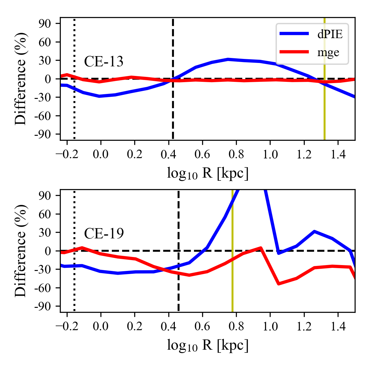
Figure 2: Difference between recovered and true surface luminosity profiles for CE-13 and CE-19. Blue lines represent the difference between the dPIE and the true profiles. Red lines show the difference between the MGE and the true profiles. The vertical yellow lines indicate the outermost radius at which kinematical data are available, which is 21 kpc unless affected by satellites along the line-of-sight. The vertical dashed lines mark the Power et al. 2003 radius and the vertical dotted lines the softening length.

For JAM we also assume that the dark matter halo follows a gNFW profile and the density distribution of the gNFW dark matter halo is also expressed as an MGE in the JAM routines.

By requiring that the predicted $v_{\rm rms}$ should be a good match to the mock galaxy’s $v_{\rm rms}$, we can estimate the following six parameters:

1. the inclination angle, $i$, between the line of sight and the axis of symmetry;

2. the anisotropy parameter, $\beta_{z}$, in Equation (9);

3. the stellar mass-to-light ratio, $M^{*}/L$;

4. the three parameters of the dark matter halo density profile: $\rho_{\rm s}$, $r_{s}$ and $\gamma$.

3.3 Model inference with the MCMC method

According to Bayes’ theorem, the posterior likelihood for a set of parameters, p, given a set of data, d, is:

$$\text{P}(\textbf{p}|\textbf{d})=\frac{\text{P}(\textbf{d}|\textbf{p})\text{P}(\textbf{p})}{\text{P}(\textbf{d})}\>,$$ (14)

where $\text{P}(\textbf{d}|\textbf{p})$ is the likelihood and P(p) is the prior distribution of the parameters. Combining the “observational” data together with the models described above, we explore the posterior distribution of the model parameters using the Markov Chain Monte Carlo (MCMC) technique. Assuming the errors are independent and Gaussian, the likelihood of a set of parameters is proportional to e${}^{-\chi^{2}/2}$, with $\chi^{2}$ defined as:

$$\chi^{2}=\chi_{K}^{2}+\chi_{SL}^{2}+\chi^{2}_{WL},$$ (15)

where the constraints from kinematics, strong and weak lensing are described by $\chi^{2}_{K}$, $\chi_{SL}^{2}$ and $\chi^{2}_{WL}$ respectively. Here, $\chi^{2}_{SL}$ and $\chi^{2}_{WL}$ take the form

$$\chi_{SL}^{2}=\left(\frac{\Sigma(<R_{E})-\Sigma^{{}^{\prime}}(<R_{E})}{\sigma_{SL}}\right)^{2}\>,$$ (16)

and

$$\chi_{WL}^{2}=\sum_{i}\left(\frac{\Delta\Sigma(R)-\Delta\Sigma^{{}^{\prime}}(R)}{\sigma_{wl}(R)}\right)^{2},$$ (17)

respectively, where the sum is over 10 data bins. $\Sigma(<R_{E})$ is the total enclosed surface mass density, including the baryonic , dark matter and gas components, within the Einstein radius, and $\Delta\Sigma(R)$ is defined in Eq. (1); $\sigma_{SL}=0.05\Sigma^{{}^{\prime}}(<R_{E})$ and $\sigma_{wl}=0.4\Delta\Sigma^{{}^{\prime}}(R)$ are the corresponding errors. $\chi^{2}_{K}$ takes the form

$$\chi^{2}_{K}=\sum_{i}\left(\frac{v^{i}_{\rm rms}-v^{{}^{\prime}i}_{\rm rms}}{\sigma^{i}_{\rm rms}}\right)^{2}\>,$$ (18)

where the $v^{i}_{\rm rms}$ is derived through JAM, $\sigma^{i}_{\rm rms}$ is the error and the sum is over 7 data bins. Note that for the sJ model, $\chi^{2}_{K}$ is calculated by substituting the rms velocity, $v_{\rm rms}$, with the line-of-sight velocity dispersion, $\sigma_{\rm los}$.

Throughout this paper, we use primed and unprimed quantities to refer to quantities derived from recovered models and from the original C-EAGLE data, respectively. Priors for the parameters are listed in Table (1). We use uniform priors over reasonable intervals for all parameters, which are similar to those adopted by Newman et al. (2013a). Note that in this work the “best-fit” parameters are given by the median values of the posterior distributions.

Table 1: Parameter priors. Here, U[a,b] denotes a uniform distribution over the interval [a,b] and $\theta$ is the upper boundary for $cos(i$) determined from the MGE model.

Parameter	Prior	Unit
cos i	U[0, $\theta$]
$\beta$	U[-0.4, 0.4]
log10 $\rho_{s}$	U[3, 10]	M⊙
log10 rs	U[${\rm log_{10}(50)}$, 3]	kpc
$\gamma_{\rm gNFW}$	U[-1.5, 0]

4 Results

4.1 Recovered density slopes

As an example, in Fig. 3 we compare the inferred and true density profiles for CE-13. The upper and lower panels show the results for sJ and JAM respectively. For both models, the recovered density profiles agree very well with the input ones except for stars beyond around 100 kpc. Since our fiducial stellar mass model assumes a constant mass-to-light ratio and our dPIE (MGE) fit to the light distribution is restricted to 100 kpc, the discrepancy beyond this radius is to be expected. Note that although the two models give very similar profiles for CE-13, there are still differences in the inner dark matter profiles where sJ tends to overestimate the mass of dark matter.

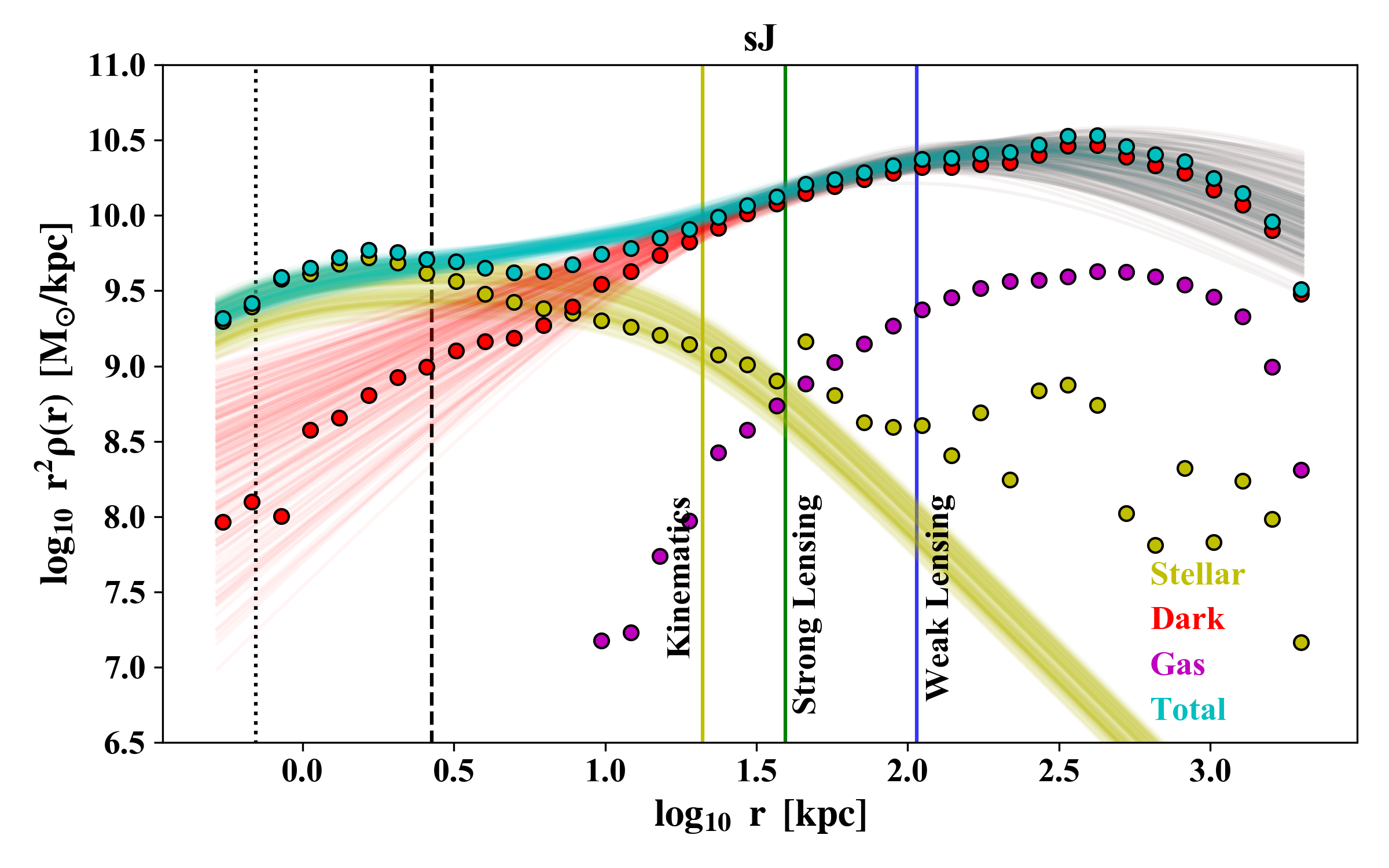
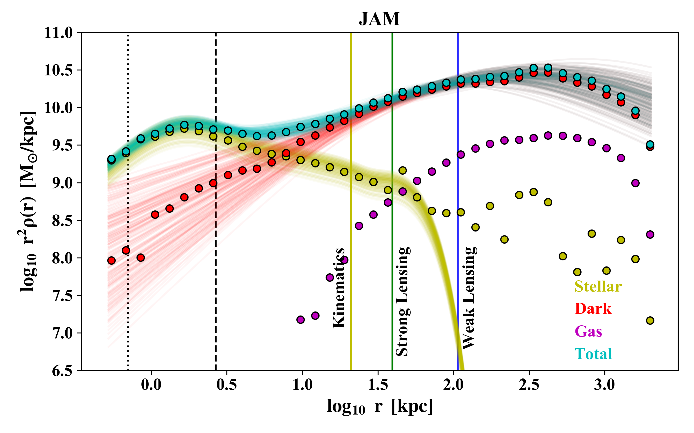
Figure 3: Reconstructed density profiles (r${}^{2}\rho$) for halo CE-13. The upper and lower panels show the reconstructed profiles using the sJ and JAM models respectively. The points show the true density profiles. The solid lines show 200 randomly selected reconstructed profiles from our MCMC samples. The dark matter, stars, gas and total density profiles are plotted in red, yellow, magenta and blue respectively. The vertical yellow line (r$=21$ kpc) marks the upper bound of the dynamical data. The vertical green line marks R_Ein. Weak lensing data exist to the right of the vertical blue line. The vertical dashed lines mark the 3D Power et al. radius and the vertical dotted lines the softening length.

In Figs. 4 and Fig. 5 we present the posterior distributions of the model parameters for sJ + lensing and JAM + lensing analyses, respectively, for CE-13. For both sJ and JAM + lensing analyses, significant degeneracies among the three parameters of the gNFW fit can be clearly seen in the contours. To compare our best-fit gNFW profiles with the input dark matter profiles, we also fit the latter between 1 kpc and R₂₀₀ to get the “true” input values of the gNFW parameters. Different choices for the radial range in the fit and the weighting scheme can lead to slightly different best-fit values because of degeneracies amongst gNFW parameters. For example, the values of $\gamma_{\rm gNFW}$ inferred from fitting to the mass profiles are systematically smaller than those inferred from fitting to the density profiles by $\sim$ 0.12. These systematic differences are well below the statistical errors of the estimates derived from kinematics + lensing analysis we have carried out.

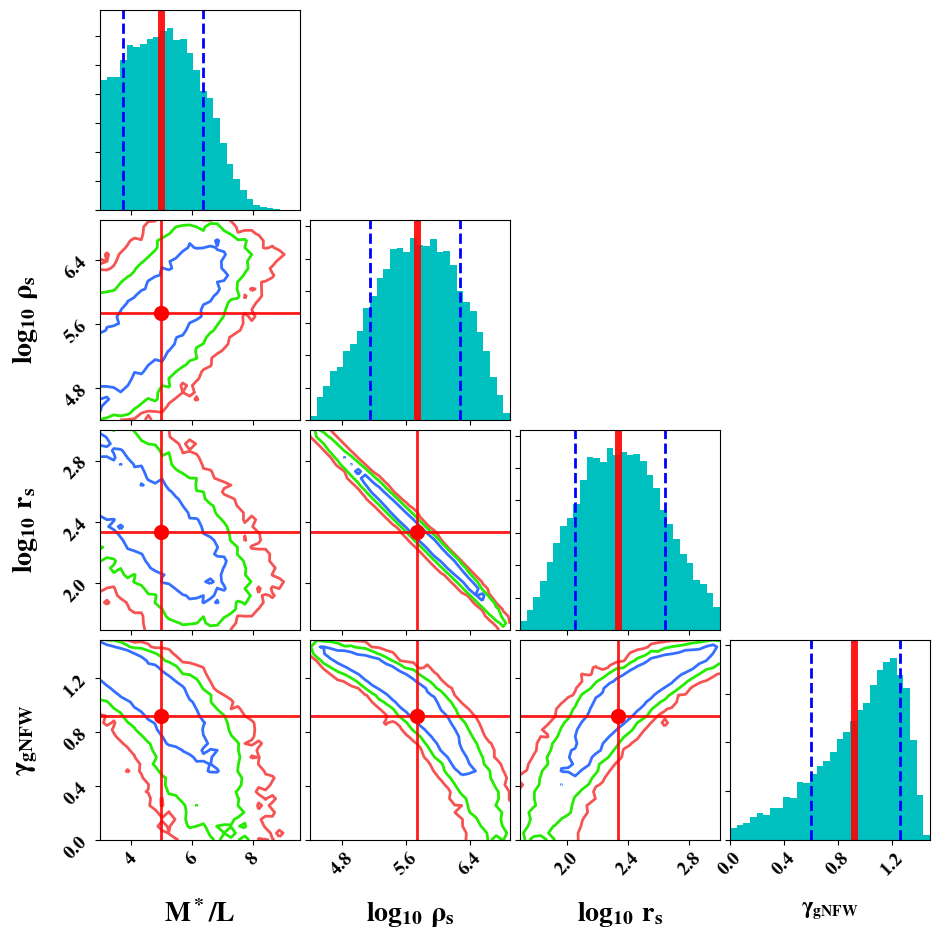
Figure 4: Posterior distributions of model parameters for the sJ + lensing analysis. In the panels with contours, true values of the parameters are marked with red dots. Blue, green and red lines represent 1-, 2- and 3$\sigma$ regions, respectively. In the marginalized distributions the input values are marked with vertical red solid lines and the 84% and 16% percentiles with vertical dashed blue lines.

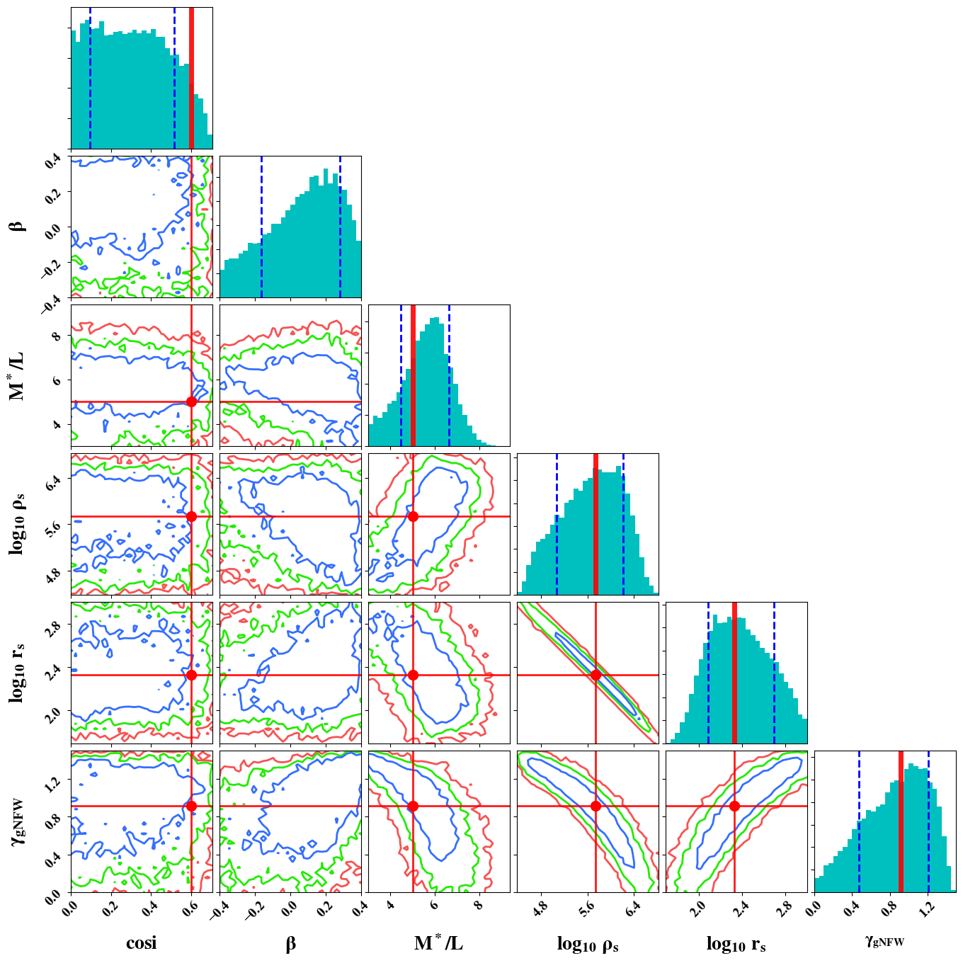
Figure 5: Posterior distributions of model parameters for the JAM + lensing analysis. In the panels with contours, the true values of the parameters are marked with red dots. Blue, green and red lines represent 1-, 2- and 3$\sigma$ regions, respectively. In the marginalized distributions the input values are marked with vertical red solid lines and the 84% and 16% percentiles with vertical dashed blue lines. The true value of $\beta$ is not shown in the plot because it lies outside the prior range; this happens only in the case of CE-13.

To compare the total inner density slope, we additionally define a mass-weighted density slope in the same way as Dutton & Treu (2014) and Newman et al. (2015):

$$\color[rgb]{0,0,0}\bar{\gamma}_{\rm dm}\equiv-\frac{1}{M(R_{e})}\int_{0}^{R_{e}}4\pi r^{2}\rho(r)\frac{d\log{\rho}}{d\log{r}}dr=3-\frac{4\pi R_{e}^{3}\rho(R_{e})}{M(R_{e})}\>,$$ (19)

where $\rho(r)$ and $M(r)$ are the cluster’s total density and mass profiles. Similarly, we define the mass-weighted dark matter density slope, $\bar{\gamma}_{\rm dm}$, by using the dark matter $\rho(r)$ and $M(r)$ density profiles in Eqn. 19. In the case where the dark matter scale radius, $r_{s}\gg R_{\rm e}$, the dark matter density slope within $R_{\rm e}$ follows a power-law distribution and the asymptotic slope $\gamma_{\rm gNFW}$ is equivalent to $\bar{\gamma}_{\rm dm}$. Note that the “true" mass-weighted slope is calculated directly from the simulation data rather than derived from a fit to the profile.

In Fig. 6 we compare the true and the best-fit values of several key parameters: $\gamma_{\rm gNFW}$, the asymptotic density slope of the dark matter halo; $\bar{\gamma}_{\rm tot}$, the mass-weighted average density slope within $R_{\rm e}$ for the total mass distribution; $\bar{\gamma}_{\rm dm}$, the mass-weighted average density slope within $R_{\rm e}$ for the dark matter distribution; $M_{\rm tot}$, the total mass within $R_{\rm e}$; $f_{\rm dm}$, the dark matter fraction within $R_{\rm e}$, for sJ + lensing analysis (left column) and JAM + lensing (right column) respectively. We denote the best-fit and true values with superscript “R" and “T" respectively.

To illustrate clearly the trend between best-fit and true values, the green dashed lines indicate equality; the red dashed lines are the linear relation between best-fit and true values. For both models, the mass-averaged dark matter density slopes, $\bar{\gamma}_{\rm dm}$, and $\gamma_{\rm gNFW}$ are reasonably well constrained. For the total mass within R_e, M_tot is overestimated by 0.1 $\sim$ 0.2 dex for many clusters. Interestingly, the best-fit total density slope, $\bar{\gamma}_{\rm tot}$, behaves very differently between the two models. JAM tends to overestimate the total density slope at small masses, while sJ systematically underestimates the total density slope at high masses. For the dark matter fraction both models provide an unbiased recovery, with sJ showing smaller variance than JAM. The parameter values in Fig. 6 are also listed in Tables 3 and 4.

To investigate whether the recovered mass depends on the dynamical state of the cluster, we classify the C-EAGLE clusters as relaxed or unrelaxed using the information provided in Table A2 of Barnes et al. (2017). A cluster is defined as relaxed if the kinetic energy of the gas is less than 10% of the total thermal energy within $R_{500}$. In Fig. 6 we use filled squares to indicate relaxed clusters and empty squares to indicate unrelaxed clusters. Overall, the quality of the recovery is independent of the dynamical state of the cluster.

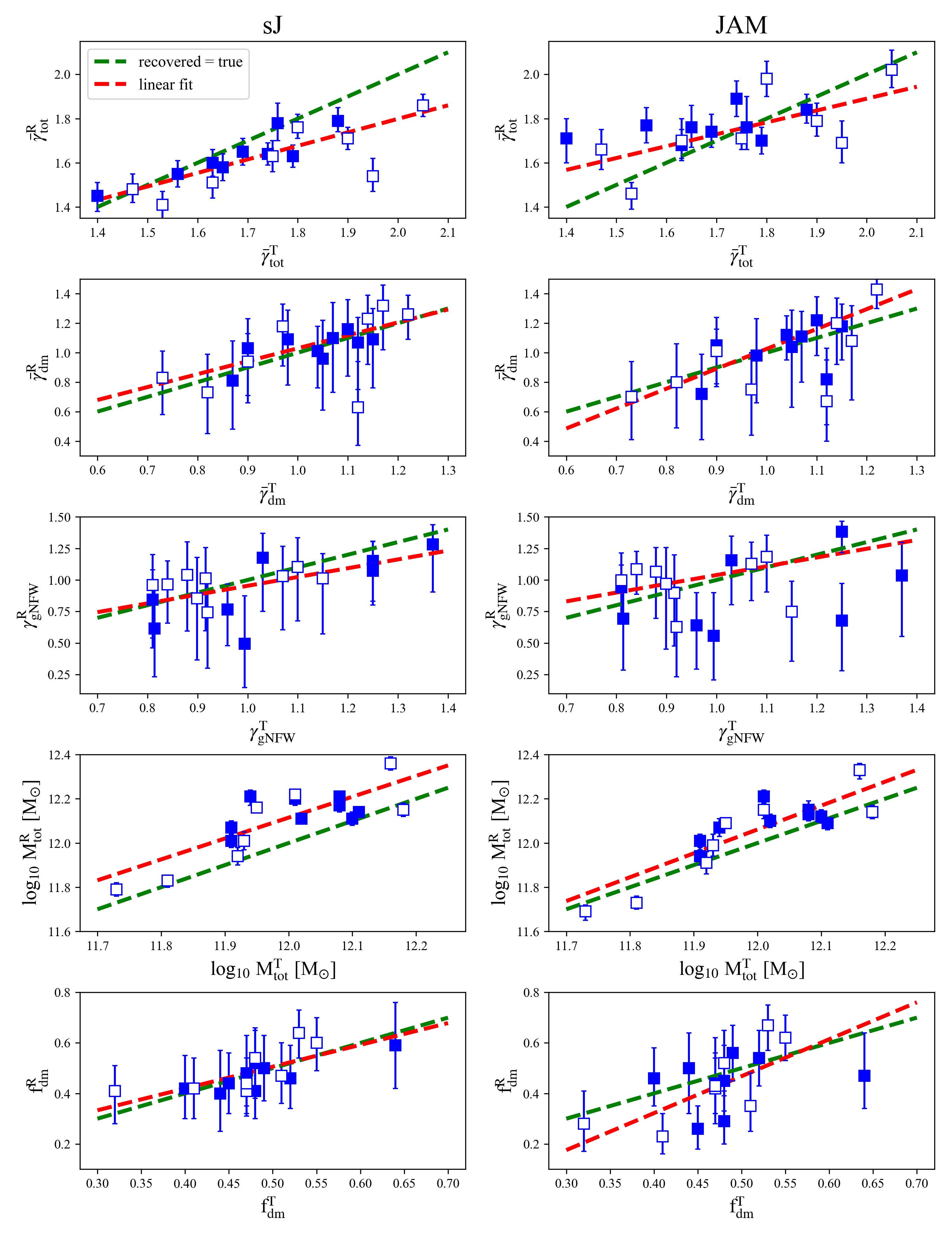
Figure 6: Comparison between the true and best-fit values of $\bar{\gamma}_{\rm tot}$, $\bar{\gamma}_{\rm dm}$, $\gamma_{\rm gNFW}$, log(M_tot) and f_dm. The left and right columns show results for sJ and JAM respectively. The $x$-axis is the true value and the $y$-axis the best-fit value. (The best-fit and true values are denoted by superscripts “R" and “T" respectively.) The solid squares represent relaxed and the empty squares unrelaxed clusters. The red dashed lines are the best linear fits to the true vs best-fit values. The green dashed lines indicate equality.

4.2 Comparison with observations

In this section, we compare our C-EAGLE mocks with the observed clusters of Newman et al. (2013a); Newman et al. (2013b, 2015). Fig. 7 shows the best-fit asymptotic dark matter density slopes, $\gamma_{\rm gNFW}$, as a function of the cluster mass, $M_{\rm 200}$, derived from our mock cluster data and from the observations of Newman et al. (2013b). For comparison, we also plot the input values of $\gamma_{\rm gNFW}$, which we derived by fitting the gNFW profile directly to the simulation data.

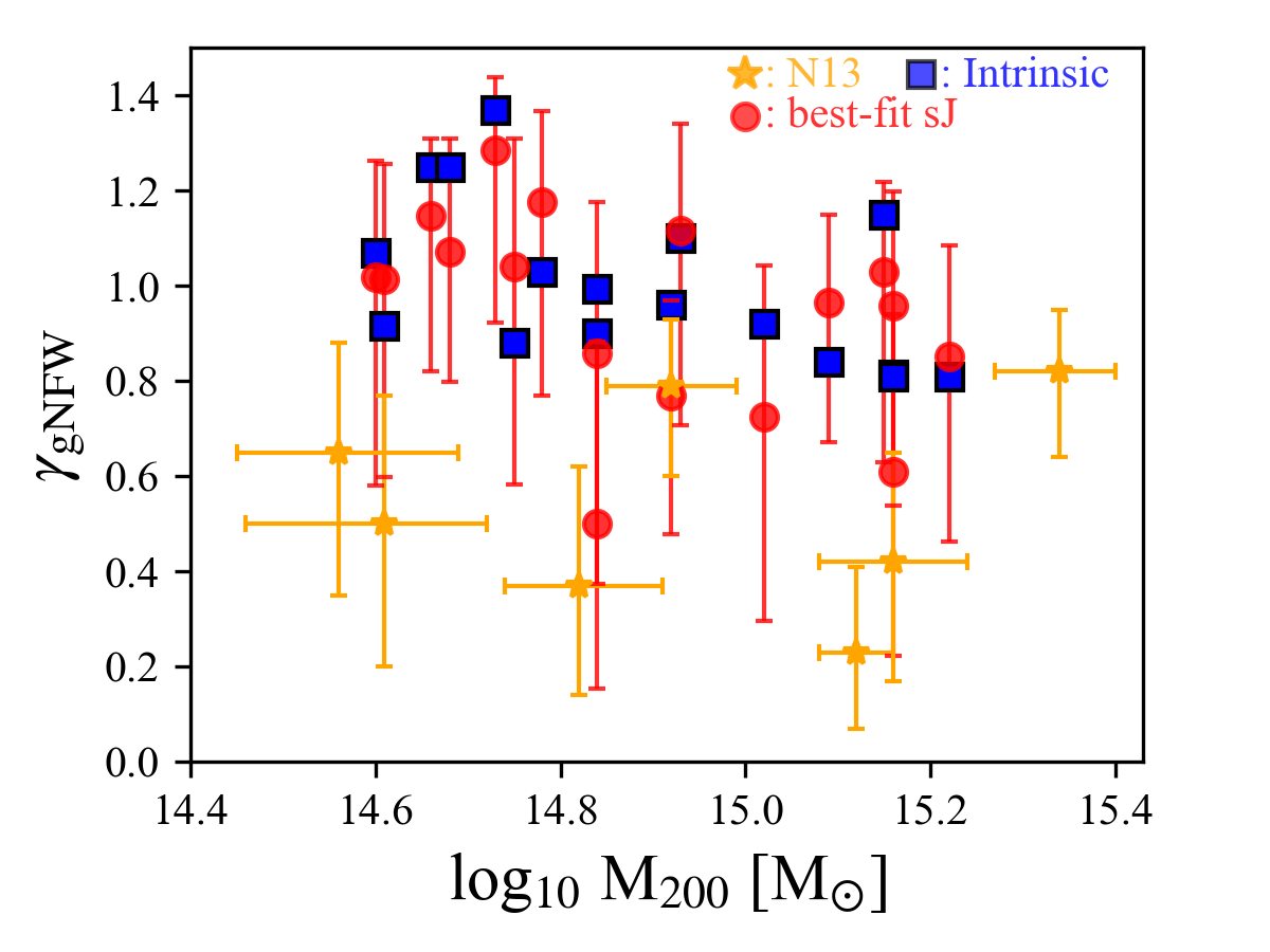
Figure 7: $\gamma_{\rm gNFW}$ as a function of M₂₀₀. Blue squares show the true values for the C-EAGLE clusters and the red circles the best-fit values from the sJeans + lensing analysis. The observational estimates from Newman et al. (2013b) are shown as yellow stars.

The true asymptotic dark matter density slopes of the C-EAGLE clusters have values $\sim 1$ at $10^{14.5}$ M_⊙ and decrease slowly to $\sim 0.8$ at $10^{15}$ M_⊙. These are significantly higher than the observational results of Newman et al. (2013b), for which the mean value is $0.50\pm 0.13$ (with an estimated systematic error of 0.14). For both the sJ and JAM + lensing analyses the recovered values of $\gamma_{\rm gNFW}$ agree well with the input ones, and both are systematically higher than those inferred from the observational data. To be specific, we use bootstrap methods to choose 7 (the same number of clusters as in Newman et al. (2013a)) asymptotic slopes, $\gamma_{\rm gNFW}$, randomly from the posterior distributions of $\gamma_{\rm gNFW}$ for all 17 clusters to derive the joint constraint on the mean value of $\gamma_{\rm gNFW}$. The method we use is different from the method used by Newman et al. (2013b) who multiplied the posterior distributions of $\gamma_{\rm gNFW}$ together, implicitly assuming that these distributions are the same for all clusters; this is not necessarily the case and the product can be strongly affected by inclusion of one or two clusters with a very different $\gamma_{\rm gNFW}$ distribution. In fact, Newman et al. (2013b) point out that excluding the cluster with the lowest $\gamma_{\rm gNFW}$ (A2537), the mean $\gamma_{\rm gNFW}$ would change by $\sim$ 40% from 0.50 to 0.69. Using the bootstrap method, we find probabilities of 3.5%, 17.1% and 49.1% for the mean value of those randomly chosen 7 asymptotic slopes to lie within the 1$\sigma$ ($0.50\pm 0.13$), 2$\sigma$ ($0.50\pm 0.26$) and 3$\sigma$ ($0.50\pm 0.39$) ranges of the Newman et al. (2013b) results, respectively. In this comparison, we combine the constraints from the kinematic, strong lensing and weak lensing data as was done by Newman et al. (2013b) and, like them, we use the sJ model for the dynamical analysis. We assume similar uncertainties for the kinematics and strong lensing as in the observational study and reasonable uncertainties for the weak lensing constraint as shown by Fig.5 in Newman et al. (2013a). Thus, the discrepancy between the observed inner density slopes and those of the C-EAGLE clusters is unlikely to be due entirely to systematics in the method itself.

Interestingly, the simulation and observational results agree well if we compare the mean values of the mass-weighted mean density slopes within the effective radius, $\bar{\gamma}_{\rm dm}$, instead of the asymptotic $\gamma_{\rm gNFW}$. Since the effective radii of the central galaxies of the C-EAGLE clusters are smaller than those of the Newman et al. (2013a) sample, roughly 44 kpc, to be consistent we measure $\bar{\gamma}_{\rm dm}$ for our clusters at 44 kpc using Eq. 19. (If not explicitly stated, $\bar{\gamma}_{\rm dm}$ is taken to mean the value at the effective radius of the C-EAGLE cluster.) In Fig. 8 we show (with dashed lines) the posterior distribution of $\bar{\gamma}_{\rm dm}$ derived by the sJ + lensing analysis for each C-EAGLE cluster. We also mark with a vertical solid black line the mean value of $\bar{\gamma}_{\rm dm}$. To explore the spread in the mean, we again use a bootstrap method to draw 7 values randomly from the posterior distribution of $\bar{\gamma}_{\rm dm}$. The solid black line in the figure shows the distribution from the bootstrap and the vertical dashed black lines its 16% and 84% percentiles. We find a mean $\bar{\gamma}_{\rm dm}=1.13\pm 0.09$. The mean and error of the true values of $\bar{\gamma}_{\rm dm}$ for the C-EAGLE clusters are shown as a cyan triangle and error bar. The yellow star and error bar show the mass-weighted mean dark matter slope for the sample of Newman et al. (2013a); Newman et al. (2013b), taken directly from Fig. 15 of Newman et al. (2015). It differs from with the true and estimated mean values for the C-EAGLE clusters by less than $\sim 1\sigma$.

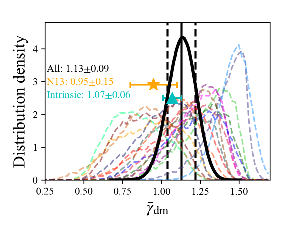
Figure 8: Marginalized posterior distributions of $\bar{\gamma}_{\rm dm}$ (at 44 kpc) obtained from the sJ + lensing analysis for each C-EAGLE cluster (dashed lines). The vertical solid black line shows the mean value of $\bar{\gamma}_{\rm dm}$. The solid curve shows the joint constraint on the mean value of $\bar{\gamma}_{\rm dm}$ and the vertical dashed lines the 16% and 84% percentiles. The yellow star with an error bar is the corresponding result of Newman et al. (2013b). The cyan triangle is the true value for our C-EAGLE sample, with the bar spanning the error in the mean. The values given in the legend are the most probable values for the mean value of $\bar{\gamma}_{\rm dm}$.

Why are the observed values of $\gamma_{\rm gNFW}$ much smaller than those from the C-EAGLE simulations, while the respective values of $\bar{\gamma}_{\rm dm}$ agree? As we discussed before, the mass-weighted density slope, $\bar{\gamma}_{\rm dm}\simeq\gamma_{\rm gNFW}$ when $r_{s}\gg R_{\rm e}$. Thus, the significant difference between the two measures of slope in the data of Newman et al. (2013a); Newman et al. (2013b) implies that the observed clusters have smaller inferred values of $r_{s}$ than the C-EAGLE clusters. To confirm this point, in the upper panel of Fig. 9, we plot the values of the gNFW scale radius as a function of M₂₀₀. For the sJ + lensing analysis, the best-fit values of $r_{s}$ agree well with the true values. But, as we can see, 4 out of the 7 clusters in Newman et al. (2013a); Newman et al. (2013b) have inferred values of the gNFW $r_{s}$ smaller than the smallest intrinsic value in the C-EAGLE sample, which is around 220 kpc. A simple interpretation of this discrepancy is that it reflects differences in the density distribution in the outer parts of the simulated and real clusters. However, since there is a degeneracy between $r_{s}$ and $\gamma_{\rm gNFW}$, the small inferred values of the gNFW $r_{s}$ could reflect the presence of a central core in the cluster dark matter distribution. To resolve this ambiguity we compare the estimated values of the NFW $r_{s}$ (from Table 8 in Newman et al. 2013a) with those found in cluster simulations (blue squares for C-EAGLE and the cyan line from Dutton & Macciò 2014). The observational estimates of the NFW $r_{s}$ are obtained exclusively from the strong and weak lensing data which pertain to regions far from the centre. As we can see, the estimated values of the NFW $r_{s}$ for the three most massive clusters in the Newman et al. sample agree well with the simulations, but those for the three smaller clusters in the sample are significantly smaller than in any of the simulated clusters, pointing to real differences in the outer density profiles of the real and simulated clusters.

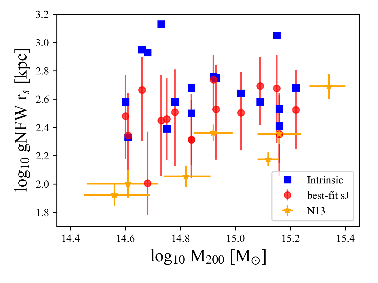
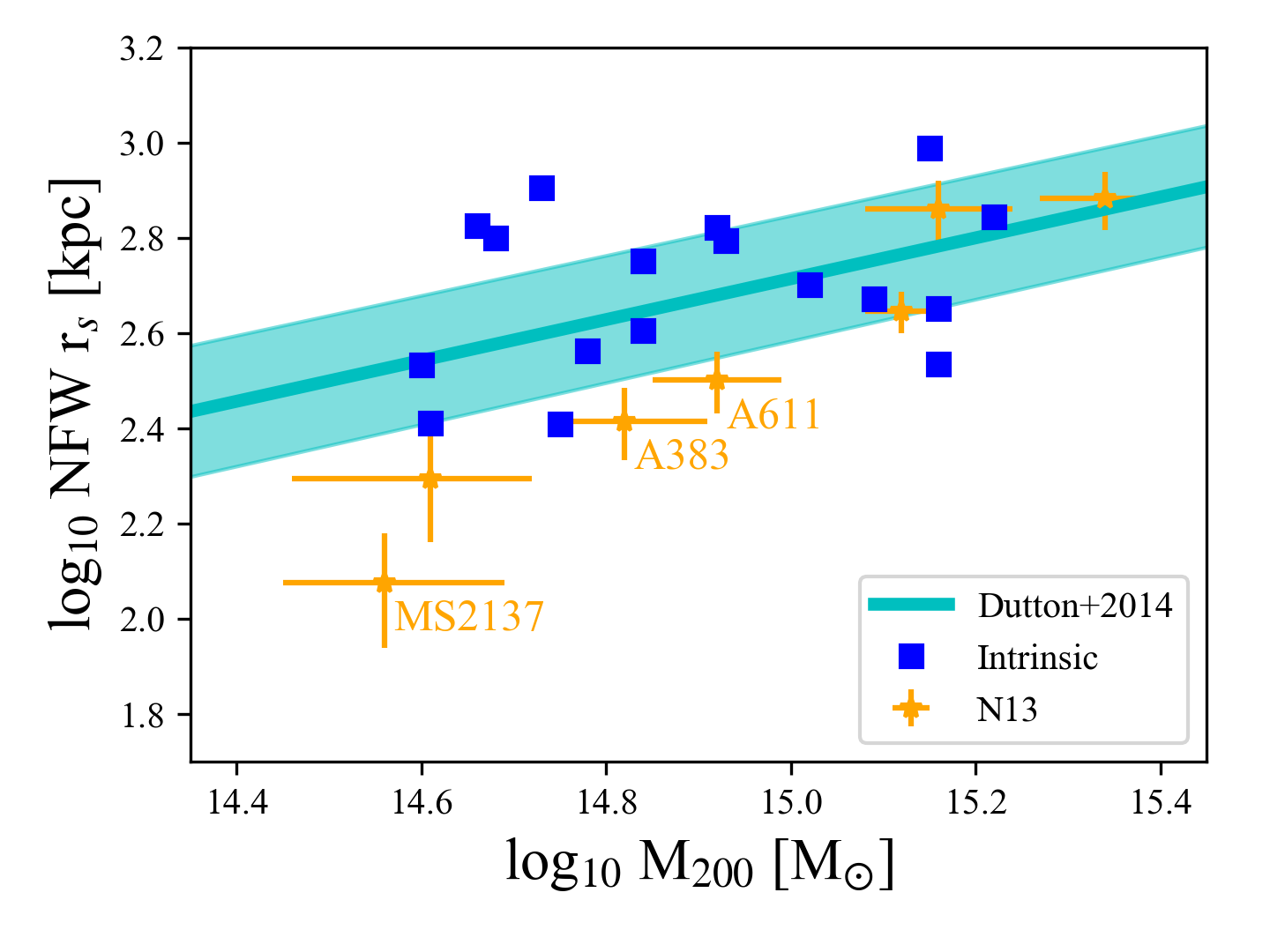
Figure 9: Upper panel: gNFW scale radius as a function of M₂₀₀. The blue squares are the true values of the gNFW $r_{s}$ for the C-EAGLE clusters; the yellow stars with error bars are the gNFW $r_{s}$ values of the Newman et al. (2013b) clusters (estimated from the Appendix of Newman et al. 2013a); and the red circles are the best-fit gNFW $r_{s}$ values for the C-EAGLE clusters from the sJ + lensing analysis. Lower panel: NFW scale radius as a function of M₂₀₀. The blue squares are the true values for the C-EAGLE clusters; the yellow stars are the values for the Newman et al. (2013a) clusters (from their Table 8). The cyan line is the mass-concentration relation for relaxed haloes at redshift 0.2 (Dutton & Macciò, 2014) , with the shaded region showing the corresponding 1-$\sigma$ scatter (Neto et al., 2007).

4.3 Importance of lensing constraints

It is worth pointing out that the lensing data plays a crucial role in constraining the mass model. Although these data probe only the outer parts of the density profile, the strong degeneracy amongst the three parameters of the gNFW profile implies that they are also important for constraining the inner parts of the profile, and help improve the precision of the decomposition of the stellar and dark mass components. Poor or biased lensing measurements may lead to the inference of incorrect dark matter slopes.

4.3.1 Tests with kinematics alone

In Fig. 10 we show the best-fit $\gamma_{\rm gNFW}$ values for the C-EAGLE clusters derived from kinematical data alone. For the sJ model, the median value of the best-fit asymptotic slope, $\gamma_{\rm gNFW}$, is 0.54, which is significantly smaller than the true value. The JAM model produces a slightly more accurate result, $\gamma_{\rm gNFW}=0.61$, but this still significantly underestimates the true density slopes.

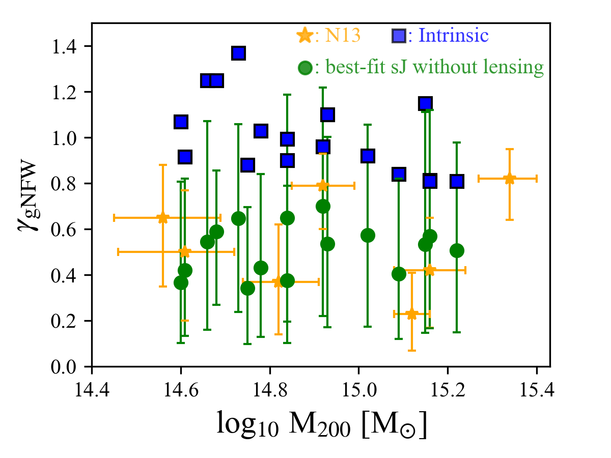
Figure 10: Comparison between the best-fit values of $\gamma_{\rm gNFW}$ for the C-EAGLE clusters from the sJ analysis alone (ignoring lensing data; green circles), the observational estimates from Newman et al. (2013b) (orange stars) and the fiducial values of C-EAGLE clusters (blue squares).

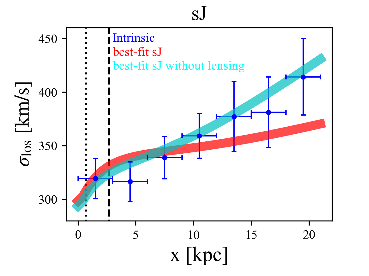
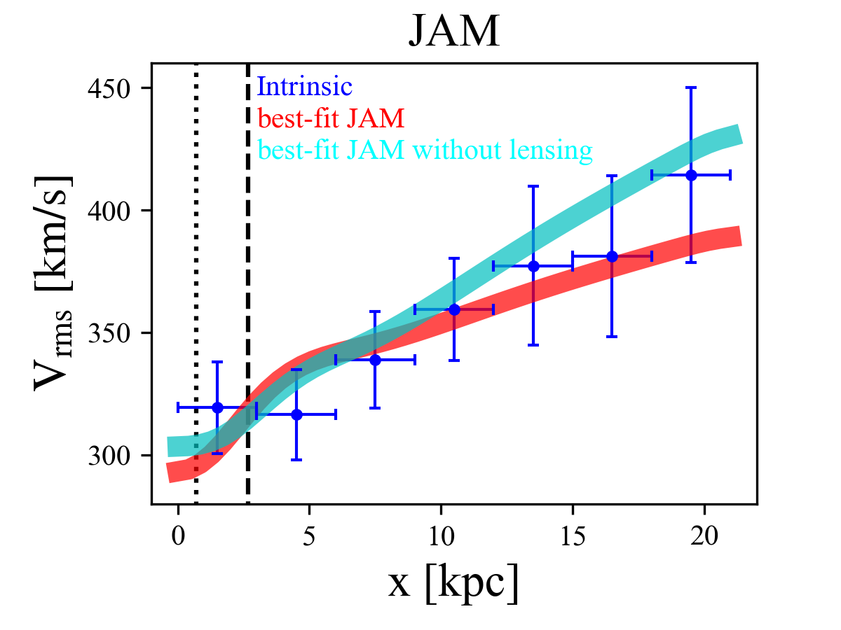
Figure 11: Comparison between true and recovered dynamical quantities for both the sJ and JAM models for CE-13. The upper panel shows the velocity dispersion of the stars and the bottom panel the rms velocity along the line-of-sight. The blue circles with error bars show the true values; the red lines represent the dispersions inferred from the full model and cyan lines those ignoring the lensing constraints. The vertical dotted lines mark the softening length and the vertical dashed lines the 3D Power et al. radius. The width of the error bars represents the size of the bins used to derive the input kinematics.

Why does dynamical modeling alone fail to reproduce the input $\gamma_{\rm gNFW}$? The reason may lie in the lack of information about the halo profile contained by the dynamical data, which are restricted to the inner halo. In Fig 11, we show dynamical quantities for CE-13 inferred from the sJ and JAM models. The blue points with error bars are the true values and the red lines are best-fit results including the lensing constraints. Both sJ and JAM fit most of the dynamical data within the errors, with JAM providing a better fit than sJ. Both models, however, underestimate the velocity dispersion at $x\sim 20$ kpc (even though they both accurately recover the true total density profiles). Ignoring the lensing constraints (cyan lines), both models overestimate the velocity dispersions at large radii. This is because, confined to the central parts of the cluster, the dynamical data alone, without the lensing data, cannot constrain the gNFW profile, especially the value of $r_{s}$. The MCMC fitting then tends to zero-in onto a shallower dark matter density profile slope than the true value, which increases the velocity dispersion in the outer regions, where it is underestimated by the full model. This explains the bias in $\gamma_{\rm gNFW}$ seen in Fig. 10.

4.3.2 Tests with biased weak lensing

In the last section we showed that the lensing measurements serve to anchor the constraints on the total density profile. Biased lensing measurements are therefore likely to lead to biased estimates of $\gamma_{\rm gNFW}$.

Interestingly, recent studies using weak lensing data of high quality find larger values of the NFW scale radius, $r_{s}$, for some of the clusters included in the sample of Newman et al. (2013a). In table 2, we compare lensing measurements of $r_{s}$, obtained from NFW fits, for three clusters by Merten et al. (2015); Umetsu et al. (2016) with the results of Newman et al. (2013a) (see Table 8 in Newman et al. (2013a), Table 6 in Merten et al. (2015) and Table 2 in Umetsu et al. (2016)). For these three clusters, the values of the scale radii measured by Newman et al. (2013a) are smaller than the more recent measurements by the other authors by 30% to $\sim$ 700%. For a comparison with simulation predictions, we have also marked those three clusters in the lower panel of Fig. 9.

To explore how the best-fit values of $\gamma_{\rm gNFW}$ are affected when the lensing measurements return a profile with too small a value of $r_{s}$, we perform the following test. We first obtain best-fit NFW profiles using unbiased weak lensing “measurements” of the C-EAGLE clusters. Next, without changing the value of M₂₀₀, we decrease the scale radius of the best-fit NFW profile by 50%, which is approximately the average difference between the results of Newman et al. (2013a) and those of Merten et al. (2015) and Umetsu et al. (2016). We then generate weak lensing measurements using these artificially biased NFW profiles with the same error bars as the fiducial ones. Finally, we combine the fiducial stellar kinematical data and strong lensing data with the artificially biased weak lensing data to constrain the mass models.

The best-fit values of $\gamma_{\rm gNFW}$ are shown as black points in Fig. 12. As may be seen, these slopes, derived assuming artificially biased weak lensing inputs, are much smaller than the true values shown in blue. They are, in fact, quite comparable to the results of Newman et al. (2013b). Of course, we do not claim that the latter are biased but our conclusions point to one possible way in which the discrepancy between the results of Newman et al. (2013b) and our simulations might be resolved.

Table 2: Comparison amongst the different lensing measurements of the NFW scale radius (in kiloparsecs) for three clusters, MS2137, A383 and A611, obtained by Newman et al. (2013a), Merten et al. (2015) and Umetsu et al. (2016) (denoted as N13, M15 and U16, respectively). For convenience, we adopt $h=0.7$

	MS2137	A383	A611
N13	119${}^{+49}_{-32}$	260${}^{+59}_{-45}$	317${}^{+57}_{-47}$
M15	686${}^{+71}_{-71}$	471${}^{+57}_{-57}$	586${}^{+86}_{-86}$
U16	800${}^{+450}_{-450}$	310${}^{+130}_{-130}$	570${}^{+210}_{-210}$

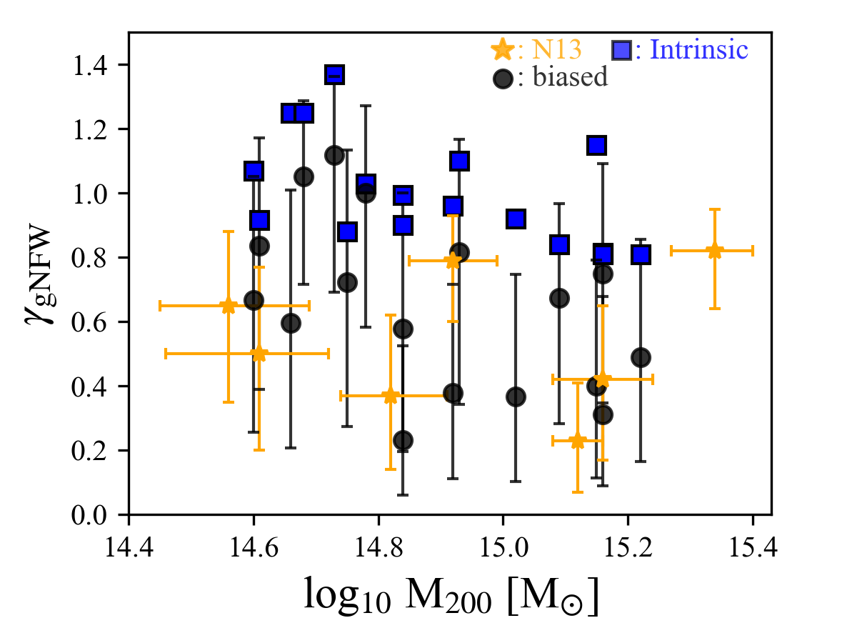
Figure 12: Comparison of the values of $\gamma_{\rm gNFW}$ inferred from biased weak lensing inputs (black points), derived by Newman et al. (2013b) (orange stars) and the actual values for C-EAGLE clusters (blue squares).

4.4 Robustness to model assumptions

In this section we consider the effect of various model assumptions on the estimates of the inner dark matter slope.

4.4.1 Mass-to-light ratio

In the preceding analysis we made use of our fiducial mock data in which a constant mass-to-light ratio was assumed when generating the surface brightness map of the central galaxy. However, this may not apply in the real Universe. To explore the sensitivity of our results to this assumption, we built another set of mocks, this time using the $r$-band luminosity calculated with the photometric method of Trayford et al. (2015). We performed the same analysis on this new set of mocks, still assuming a constant $M^{*}/L$. The difference between these results and those from our fiducial model reflects the uncertainties introduced by the simple assumption of constant $M^{*}/L$.

In Fig. 13 we compare the joint constraints on the mean $\bar{\gamma}_{\rm dm}$ (at 44 kpc) from our mock data using the sJ + lensing model, assuming a constant $M^{*}/L$, for both, mocks constructed making this same assumption and mocks constructed using the photometric model of Trayford et al. (2015). The inferred mean $\bar{\gamma}_{\rm dm}$ in the latter case is only about 3% smaller than in the standard case. These results indicate that the assumption of a constant $M^{*}/L$ is reasonable for the analysis of the inner dark matter density profiles in these massive clusters.

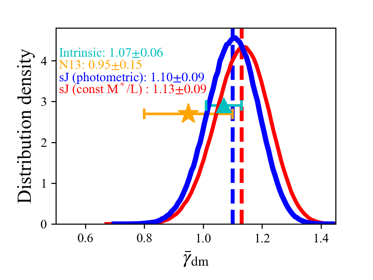
Figure 13: Comparison of the joint constraints on the mean $\bar{\gamma}_{\rm dm}$ (at 44 kpc) from mock data constructed either assuming a constant ${M^{*}/L}$ (red) or the photometric model of Trayford et al. (2015) (blue). Results are shown for sJ + lensing modelling, assuming in both cases that ${M^{*}/L}$ is constant. The yellow symbol and error bar show the observational result of Newman et al. (2013b), while the cyan symbol and error bar correspond to the true C-EAGLE result. The values quoted in the legend are the most probable values of the mean $\bar{\gamma}_{\rm dm}$ derived from the corresponding test.

4.4.2 Shape of the central galaxy

When modeling the central stellar dynamics by solving the Jeans equations, we assumed the galaxy to have either a spherical or an oblate shape. A spherical shape for the central galaxy is assumed in the sJ model, while an oblate shape is assumed in the fiducial JAM model. Although this oblateness assumption is valid for most early type galaxies, it does not apply to the most massive ones (e.g. Li et al., 2016, 2017). To be consistent with previous analyses, we assumed oblateness in our application of the JAM. In the upper and lower panel of Fig. 14 we show the error in the inferred mass-weighted slope of the dark matter density profile, $\delta\bar{\gamma}_{\rm dm}=(\bar{\gamma}_{\rm dm}^{{}^{\prime}}-\bar{\gamma}_{\rm dm})/\bar{\gamma}_{\rm dm}$ (where, as before, $\bar{\gamma}^{{}^{\prime}}_{\rm dm}$ denotes the best-fit value and $\bar{\gamma}_{\rm dm}$ the true value), as a function of the triaxiality parameter, $T\equiv\frac{a^{2}-b^{2}}{a^{2}-c^{2}}$ (Binney & Tremaine, 2008) for both the sJ and JAM models.

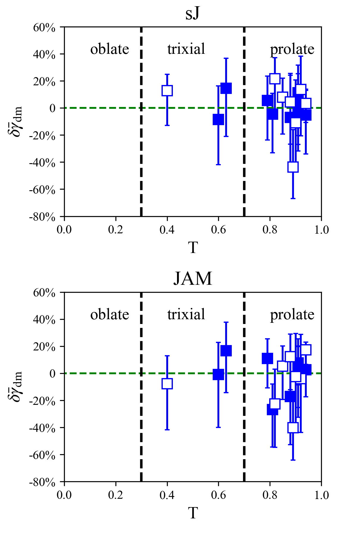
Figure 14: $\delta\bar{\gamma}_{\rm dm}$ as a function of the triaxiality parameter. The solid squares show relaxed clusters and the empty squares unrelaxed clusters.

We compute the triaxiality parameter of the galaxy using the reduced inertia tensor defined as:

$$I_{ij,k+1}=\frac{\sum\limits_{n}M_{n}x_{i,n}x_{j,n}/r_{n,k}^{2}}{\sum\limits_{n}M_{n}}\>,$$ (20)

where $i,j\in\{x,y,z\}$ and the summation is over the stars within 25 kpc, (which is slightly larger than the region with kinematical data and around 2 R_e for our sample. Here, $r_{n,k}$ is defined as the $k$-th iteration value of the radius,

$$r_{n,k}=\sqrt{x_{n}^{2}+y_{n}^{2}/q^{2}+z_{n}^{2}/s^{2}}\>,$$ (21)

where $q=b/a$ and $s=c/a$ (assuming the lengths of the three major axes are $a$, $b$, $c$ and $a\geq b\geq c$) are the square root of the ratios of the reduced inertia tensor eigenvalues. We iteratively calculate the reduced inertia tensor and the values of $q$ and $s$, deriving the triaxiality parameter from the stable $q$ and $s$ values.

If $s\geq 0.9$, then the galaxy is close to spherical and, if $s\leq 0.9$, we can classify the shape into three categories: oblate for $T\leq 0.3$, prolate for $T\geq 0.7$ and triaxial in between. All of our clusters have $s\leq 0.9$. From Fig. 14, we find that most of the cluster central galaxies have a prolate shape. Interestingly, although the shapes are not consistent with the assumption of the JAM or the sJ model, we do not find a correlation between the accuracy of the estimate of $\bar{\gamma}_{\rm dm}$ and the triaxiality parameter.

To explore further the model dependence on the galaxy shape, we rotate all of our galaxies in three different directions, so that the line-of-sight direction is aligned with the major, intermediate and minor axes respectively, and repeat the kinematics + lensing analysis. We show the best-fit $\gamma_{\rm gNFW}$ in different directions as a function of M₂₀₀ in Fig. 15. We see that for both models looking along intermediate and minor axes gives similar $\gamma_{\rm gNFW}$ distributions, while looking along the longest axis gives larger best-fit values of $\gamma_{\rm gNFW}$ than for the two other directions. The probability of drawing 7 asymptotic slope values from their posterior distributions with mean value lying within the 1$\sigma$ range of the observational result ($0.50\pm 0.13$) are 17.3%, 5.7% and 1.5% when viewing along minor, intermediate and major axes, respectively.

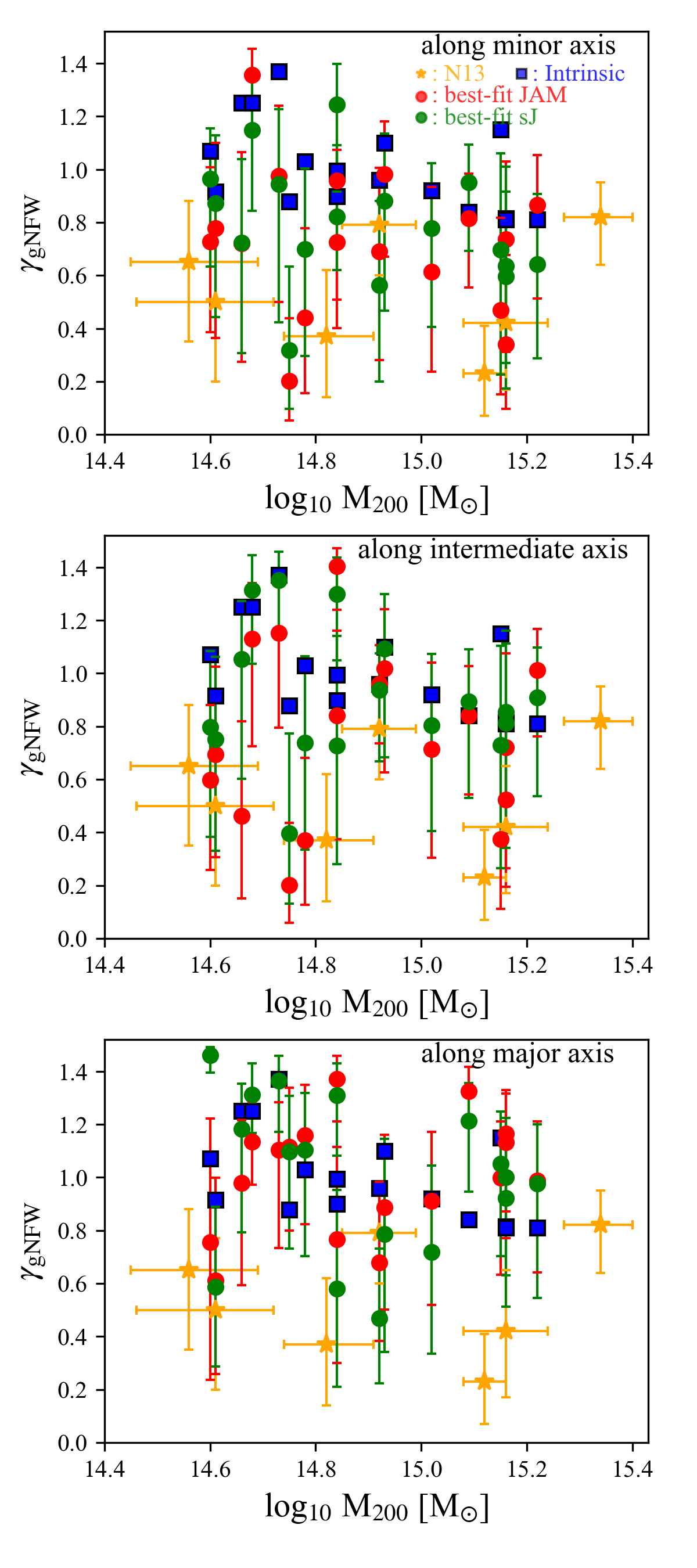
Figure 15: Values of $\gamma_{\rm gNFW}$ for C-EAGLE clusters viewed from different directions. The upper, middle and lower panels show results when viewing the central galaxies along the minor, intermediate and major axis, respectively. Blue squares are the true C-EAGLE values and the yellow stars the measured values of Newman et al. (2013b). Red and green circles are results from the JAM and sJ model respectively.

4.4.3 Velocity anisotropy

We also test the dependence of the model on the velocity anisotropy. Schaller et al. (2015b) suggested that the discrepancy between the dark matter density profile slopes in the observed clusters and in the EAGLE simulations might be due to incorrect assumptions for the velocity anisotropy parameters. In the sJ modeling, the velocity anisotropy is assumed to be zero, while in JAM it is assumed to be constant in the $z$ cylindrical coordinate.

In Fig. 16 we plot the error in the estimates of $\bar{\gamma}_{\rm dm}$ as a function of the anisotropy parameter, $\beta$, of the C-EAGLE clusters for both the sJ and JAM cases. The anisotropy in cylindrical coordinates, $\beta_{\rm JAM}$ ($\beta_{z}$), is computed as

$$\beta_{\rm JAM}=1-\frac{\overline{v_{z}^{2}}}{\overline{v_{R}^{2}}}\>,$$ (22)

where the $z$-axis is aligned with the minor axis of the galaxy. The anisotropy parameter for the spherical Jeans model is computed as:

$$\beta_{\rm sJ}=1-\frac{\overline{v_{\theta}^{2}}}{\overline{v_{r}^{2}}}\>,$$ (23)

where $\overline{v_{\theta}^{2}}=\overline{v_{\phi}^{2}}$. There is significant galaxy to galaxy scatter in the anisotropy parameter value but we do not find a significant trend of $\delta\bar{\gamma}_{\rm dm}$ with $\beta$.

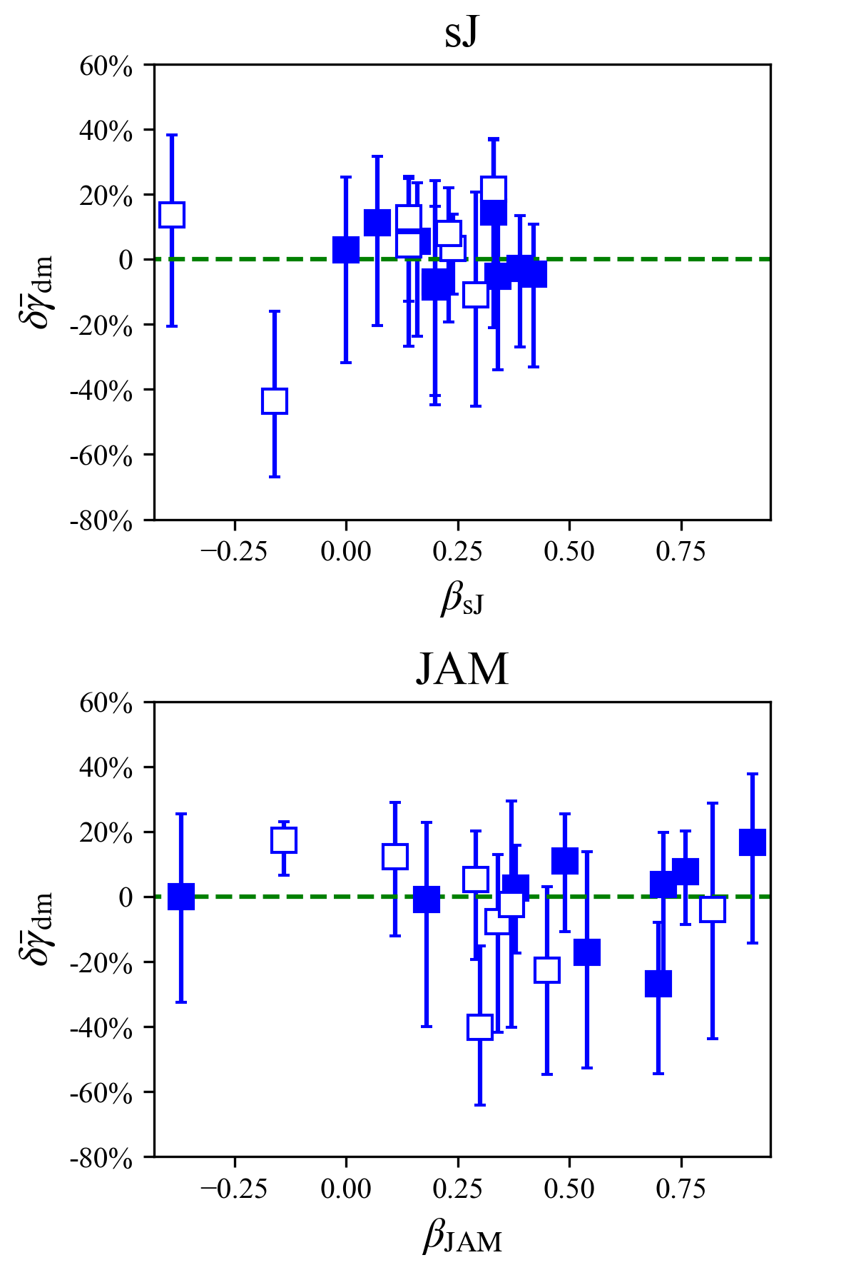
Figure 16: $\delta\bar{\gamma}_{\rm dm}$ as a function of the anisotropy parameter, $\beta$. The solid squares show relaxed clusters and the empty squares unrelaxed clusters.

5 Summary and Discussion

We have investigated the accuracy of techniques for inferring the inner density profiles of massive galaxy clusters from a combination of stellar kinematics and gravitational lensing data. We constructed mock datasets from 17 clusters in the C-EAGLE hydrodynamical simulations (Barnes et al., 2017; Bahé et al., 2017), whose masses are comparable to those of the seven clusters studied by Newman et al. (2013a) (with a mean M${}_{\rm 200}\sim 1\times 10^{15}$ $\rm{M}_{\odot}$). We performed a stellar dynamical and lensing analysis on the mock datasets. For the former we used two different methods: the spherical Jeans model, which was the method used by Newman et al. (2013a); Newman et al. (2013b), and the Jeans anistropic model. Our findings can be summarized as follows:

• The values of the inner asymptotic slope of a “generalized” NFW density profile, $\gamma_{\rm gNFW}$, estimated using the kinematics + lensing analysis on the mock data agree reasonably well with the input values indicating that, in principle, the method is accurate and unbiased.

• The dark matter asymptotic density slopes, $\gamma_{\rm gNFW}$, of massive C-EAGLE clusters are steeper than those inferred by Newman et al. (2013a); Newman et al. (2013b) for the observed clusters. The C-EAGLE clusters have $\gamma_{\rm gNFW}\sim 1$, whereas Newman et al. (2013b) find $\gamma_{\rm gNFW}\sim 0.5$ for their clusters, as shown in Fig. 7.

• The inner density profile can also be characterized by the mean mass-weighted dark matter density slope, $\bar{\gamma}_{\rm dm}$, averaged within the effective optical radius of the central galaxy. To compare our results with observations, we derive this average slope within 44 kpc, which is approximately the effective radius of the clusters of Newman et al. (2013a). Taking errors into account, the average slopes from C-EAGLE clusters agree with the observed ones (see Fig. 8).

• The different conclusions reached when using the two different measures of inner dark matter density profile slope can be traced back to different values of the characteristic halo radius, $r_{s}$, in the C-EAGLE and observed clusters. The values of $r_{s}$ inferred for the Newman et al. (2013a) sample are significantly smaller than the values for the clusters in the simulations (see Fig. 9). The smaller the $r_{s}$, the faster the dark matter density slope varies within the effective radius and thus the larger the difference between the asymptotic and mass-weighted values.

• We find that there is a strong degeneracy between the asymptotic gNFW slope, $\gamma_{\rm gNFW}$, and the scale radius, $r_{s}$ (or, equivalently, the scale density, $\rho_{\rm s}$; see Figs. 4 and 5). As a result, the gravitational lensing data which directly probe the cluster mass distribution at large distances also play a role in constraining the inner profiles. To assess the importance of lensing data, we repeated our analysis of the C-EAGLE clusters in two ways. Firstly, we ignored lensing and used only stellar kinematical data. We found that, in this case, the dark matter density slopes are significantly underestimated (see Fig. 10). This is probably because, as shown in Fig. 11, not including constraints from lensing loses the anchor point in the outer regions of the cluster and a nearly constant density dark matter core is then preferred to account for the steeply raising observed stellar velocity dispersion profile (which otherwise the stellar dynamical models considered here would have difficulty matching).

  Secondly, we kept the stellar kinematical and strong lensing mock data unchanged, but artificially biased the weak lensing mock data to correspond to a profile with a 50% smaller value of the NFW $r_{s}$. We found that, in this case, the best-fit $\gamma_{\rm gNFW}$ values are significantly underestimated and are, in fact, quite comparable with the values estimated by Newman et al. (2013a); Newman et al. (2013b). We noted that for three clusters, the NFW scale radii measured by Newman et al. (2013a) are much smaller than the more recent measurements carried out by Merten et al. (2015) and Umetsu et al. (2016). Based on these tests, we suggest that stellar kinematical data combined with lensing measurements from the more recent observations would alleviate the discrepancy between the observed dark matter density slopes and the theoretical predictions. We also note, however, that the haloes of three of the observed clusters have scale radii similar to those in the simulations (lower panel of Fig. 9), so biased lensing results may not be the whole story behind the tension.

• We also applied our sJ + lensing and JAM + lensing analyses to clusters viewed from their minor, intermediate and major axes. We found that the best-fit $\gamma_{\rm gNFW}$ tends to be larger than the true value when the cluster is viewed from the direction of the major axis. If the observed sample were biased in this way, the discrepancy with the C-EAGLE clusters would be even larger.

• We tested the robustness of the method to the assumptions of a constant stellar mass-to-light ratio and an isotropic velocity anisotropy and found the method to be fairly insensitive to these assumptions.

  In summary, while according to one measurement (the mean inner slope of the dark matter density profile) the observational data agree with the simulations, according to another (the asymptotic slope) they do not. These two measures differ in the way they weight different regions of the mass distribution in the cluster. The asymptotic slopes are extrapolations that rely on the innermost data points whereas the mean slopes may be more robust. The inferred asymptotic slopes are degenerate with the scale radius (or the scale density) of the halo and thus they can be strongly affected by the lensing data; a poor or biased measurement of the lensing constraints can lead to significantly smaller asymptotic slopes. Thus, although some tension between the simulations and the data remains, this does not necessarily imply a fatal inconsistency between the two.

Data availability

The data underlying this article will be shared on reasonable request to the corresponding author.

Appendix A Tables for key recovered parameters

We list best-fit and true values for six key parameters in Table 3 and Table 4 for sJ and JAM + lensing analysis, respectively.

Table 3: Comparison between true and best-fit parameters obtained from sJ plus lensing analysis. The best-fit and true values are denoted with superscript "R" and "T" respectively. $\bar{\gamma}_{\rm tot}$ and $\bar{\gamma}_{\rm dm}$ are the mass-weighted slope of total density profiles and dark matter density profiles and $\gamma_{\rm gNFW}$ is the asymptotic dark matter density slope. M^∗ and M_tot are the stellar and total mass enclosed within the stellar effective radius, R_e. The unit of mass is M_⊙. f_dm is the dark matter mass fraction witnin R_e. Errors are calculated as 84 and 16 percentiles.

	$\bar{\gamma}^{\rm T}_{\rm tot}$	$\bar{\gamma}^{\rm R}_{\rm tot}$	$\bar{\gamma}^{\rm T}_{\rm dm}$	$\bar{\gamma}^{\rm R}_{\rm dm}$	$\gamma^{\rm T}_{\rm gNFW}$	$\gamma^{\rm R}_{\rm gNFW}$	log10 M∗T	log10 M∗R	log10 M${}^{\rm T}_{\rm tot}$	log10 M${}^{\rm R}_{\rm tot}$	f${}^{\rm T}_{\rm dm}$	f${}^{\rm R}_{\rm dm}$
CE-12	1.79	1.63${}^{+0.05}_{-0.05}$	1.15	1.09${}^{+0.21}_{-0.33}$	1.07	1.03${}^{+0.24}_{-0.42}$	11.62	11.76${}^{+0.09}_{-0.13}$	11.91	12.07${}^{+0.03}_{-0.04}$	0.49	0.50${}^{+0.13}_{-0.13}$
CE-13	1.69	1.65${}^{+0.06}_{-0.06}$	0.98	1.09${}^{+0.20}_{-0.31}$	0.92	1.01${}^{+0.24}_{-0.41}$	11.63	11.69${}^{+0.10}_{-0.13}$	11.91	12.01${}^{+0.02}_{-0.03}$	0.48	0.52${}^{+0.13}_{-0.14}$
CE-14	1.80	1.76${}^{+0.06}_{-0.05}$	0.97	1.18${}^{+0.15}_{-0.27}$	1.25	1.15${}^{+0.16}_{-0.32}$	11.58	11.59${}^{+0.08}_{-0.10}$	11.81	11.83${}^{+0.02}_{-0.03}$	0.41	0.42${}^{+0.12}_{-0.12}$
CE-15	2.05	1.86${}^{+0.05}_{-0.05}$	1.17	1.32${}^{+0.14}_{-0.30}$	1.37	1.28${}^{+0.16}_{-0.38}$	11.56	11.57${}^{+0.09}_{-0.09}$	11.73	11.79${}^{+0.03}_{-0.03}$	0.32	0.41${}^{+0.10}_{-0.13}$
CE-16	1.76	1.78${}^{+0.09}_{-0.08}$	1.07	1.10${}^{+0.24}_{-0.37}$	0.88	1.04${}^{+0.26}_{-0.45}$	11.69	11.99${}^{+0.11}_{-0.15}$	11.94	12.21${}^{+0.03}_{-0.04}$	0.44	0.40${}^{+0.17}_{-0.15}$
CE-17	1.75	1.63${}^{+0.07}_{-0.07}$	1.22	1.26${}^{+0.13}_{-0.17}$	1.25	1.07${}^{+0.23}_{-0.27}$	11.63	11.72${}^{+0.11}_{-0.12}$	11.95	12.16${}^{+0.02}_{-0.02}$	0.53	0.64${}^{+0.09}_{-0.10}$
CE-18	1.65	1.58${}^{+0.06}_{-0.06}$	1.05	0.96${}^{+0.26}_{-0.35}$	0.90	0.85${}^{+0.32}_{-0.49}$	11.73	11.83${}^{+0.09}_{-0.14}$	12.02	12.11${}^{+0.02}_{-0.02}$	0.47	0.48${}^{+0.15}_{-0.13}$
CE-19	1.95	1.54${}^{+0.08}_{-0.07}$	1.12	0.63${}^{+0.31}_{-0.26}$	0.99	0.50${}^{+0.38}_{-0.35}$	11.65	11.71${}^{+0.06}_{-0.08}$	11.92	11.94${}^{+0.04}_{-0.04}$	0.47	0.41${}^{+0.13}_{-0.10}$
CE-20	1.90	1.71${}^{+0.05}_{-0.05}$	1.14	1.23${}^{+0.16}_{-0.31}$	1.03	1.18${}^{+0.19}_{-0.43}$	11.72	11.88${}^{+0.10}_{-0.14}$	12.01	12.22${}^{+0.02}_{-0.02}$	0.48	0.54${}^{+0.12}_{-0.13}$
CE-21	1.88	1.79${}^{+0.06}_{-0.05}$	1.10	1.16${}^{+0.20}_{-0.32}$	1.10	1.10${}^{+0.23}_{-0.43}$	11.86	11.97${}^{+0.08}_{-0.11}$	12.08	12.21${}^{+0.02}_{-0.02}$	0.40	0.42${}^{+0.13}_{-0.12}$
CE-22	1.56	1.55${}^{+0.06}_{-0.06}$	0.87	0.81${}^{+0.27}_{-0.33}$	0.92	0.74${}^{+0.30}_{-0.44}$	11.81	11.87${}^{+0.07}_{-0.10}$	12.10	12.11${}^{+0.03}_{-0.03}$	0.48	0.41${}^{+0.14}_{-0.11}$
CE-23	1.47	1.48${}^{+0.07}_{-0.06}$	0.73	0.83${}^{+0.18}_{-0.25}$	0.96	0.77${}^{+0.20}_{-0.29}$	11.62	11.73${}^{+0.07}_{-0.10}$	11.93	12.01${}^{+0.04}_{-0.04}$	0.51	0.47${}^{+0.13}_{-0.11}$
CE-24	1.63	1.60${}^{+0.06}_{-0.06}$	1.04	1.01${}^{+0.17}_{-0.25}$	0.84	0.97${}^{+0.18}_{-0.31}$	11.76	11.90${}^{+0.08}_{-0.12}$	12.08	12.17${}^{+0.02}_{-0.03}$	0.52	0.46${}^{+0.13}_{-0.12}$
CE-25	1.74	1.64${}^{+0.05}_{-0.05}$	1.12	1.07${}^{+0.17}_{-0.32}$	1.15	1.01${}^{+0.20}_{-0.44}$	11.85	11.89${}^{+0.08}_{-0.11}$	12.11	12.14${}^{+0.02}_{-0.02}$	0.45	0.44${}^{+0.12}_{-0.12}$
CE-26	1.63	1.51${}^{+0.07}_{-0.07}$	0.82	0.73${}^{+0.26}_{-0.28}$	0.82	0.62${}^{+0.33}_{-0.38}$	11.90	11.89${}^{+0.07}_{-0.10}$	12.18	12.15${}^{+0.03}_{-0.03}$	0.47	0.44${}^{+0.12}_{-0.10}$
CE-27	1.40	1.45${}^{+0.06}_{-0.07}$	0.90	1.03${}^{+0.20}_{-0.32}$	0.81	0.96${}^{+0.24}_{-0.42}$	11.56	11.81${}^{+0.15}_{-0.23}$	12.01	12.20${}^{+0.02}_{-0.03}$	0.64	0.59${}^{+0.17}_{-0.17}$
CE-28	1.53	1.41${}^{+0.06}_{-0.07}$	0.90	0.94${}^{+0.19}_{-0.28}$	0.81	0.85${}^{+0.23}_{-0.38}$	11.81	11.96${}^{+0.09}_{-0.11}$	12.16	12.36${}^{+0.03}_{-0.03}$	0.55	0.60${}^{+0.10}_{-0.11}$

Table 4: Comparison between true and best-fit parameters obtained from JAM plus lensing analysis. Notations are the same as Table 3.

	$\bar{\gamma}^{\rm T}_{\rm tot}$	$\bar{\gamma}^{\rm R}_{\rm tot}$	$\bar{\gamma}^{\rm T}_{\rm dm}$	$\bar{\gamma}^{\rm R}_{\rm dm}$	$\gamma^{\rm T}_{\rm gNFW}$	$\gamma^{\rm R}_{\rm gNFW}$	log10 M∗T	log10 M∗R	log10 M${}^{\rm T}_{\rm tot}$	log10 M${}^{\rm R}_{\rm tot}$	f${}^{\rm T}_{\rm dm}$	f${}^{\rm R}_{\rm dm}$
CE-12	1.79	1.70${}^{+0.06}_{-0.06}$	1.15	1.18${}^{+0.15}_{-0.23}$	1.07	1.13${}^{+0.17}_{-0.30}$	11.62	11.65${}^{+0.08}_{-0.10}$	11.91	12.01${}^{+0.03}_{-0.04}$	0.49	0.56${}^{+0.11}_{-0.11}$
CE-13	1.69	1.74${}^{+0.08}_{-0.07}$	0.98	0.98${}^{+0.25}_{-0.32}$	0.92	0.90${}^{+0.31}_{-0.42}$	11.63	11.68${}^{+0.07}_{-0.10}$	11.91	11.94${}^{+0.04}_{-0.04}$	0.48	0.45${}^{+0.14}_{-0.12}$
CE-14	1.80	1.98${}^{+0.08}_{-0.08}$	0.97	0.75${}^{+0.25}_{-0.31}$	1.25	0.69${}^{+0.31}_{-0.40}$	11.58	11.61${}^{+0.04}_{-0.05}$	11.81	11.73${}^{+0.03}_{-0.03}$	0.41	0.23${}^{+0.09}_{-0.07}$
CE-15	2.05	2.02${}^{+0.09}_{-0.08}$	1.17	1.08${}^{+0.24}_{-0.40}$	1.37	1.03${}^{+0.26}_{-0.46}$	11.56	11.54${}^{+0.07}_{-0.08}$	11.73	11.69${}^{+0.03}_{-0.04}$	0.32	0.28${}^{+0.13}_{-0.11}$
CE-16	1.76	1.76${}^{+0.14}_{-0.10}$	1.07	1.11${}^{+0.17}_{-0.31}$	0.88	1.07${}^{+0.20}_{-0.36}$	11.69	11.77${}^{+0.14}_{-0.15}$	11.94	12.07${}^{+0.04}_{-0.04}$	0.44	0.50${}^{+0.14}_{-0.18}$
CE-17	1.75	1.71${}^{+0.05}_{-0.05}$	1.22	1.43${}^{+0.07}_{-0.13}$	1.25	1.39${}^{+0.08}_{-0.16}$	11.63	11.62${}^{+0.11}_{-0.12}$	11.95	12.09${}^{+0.02}_{-0.02}$	0.53	0.67${}^{+0.08}_{-0.10}$
CE-18	1.65	1.76${}^{+0.10}_{-0.09}$	1.05	1.04${}^{+0.25}_{-0.41}$	0.90	0.98${}^{+0.29}_{-0.53}$	11.73	11.84${}^{+0.09}_{-0.16}$	12.02	12.10${}^{+0.03}_{-0.03}$	0.47	0.44${}^{+0.18}_{-0.16}$
CE-19	1.95	1.69${}^{+0.10}_{-0.09}$	1.12	0.67${}^{+0.28}_{-0.27}$	0.99	0.55${}^{+0.34}_{-0.34}$	11.65	11.67${}^{+0.06}_{-0.07}$	11.92	11.91${}^{+0.05}_{-0.05}$	0.47	0.42${}^{+0.12}_{-0.10}$
CE-20	1.90	1.79${}^{+0.08}_{-0.07}$	1.14	1.20${}^{+0.17}_{-0.28}$	1.03	1.16${}^{+0.18}_{-0.34}$	11.72	11.84${}^{+0.08}_{-0.11}$	12.01	12.15${}^{+0.04}_{-0.04}$	0.48	0.52${}^{+0.13}_{-0.13}$
CE-21	1.88	1.84${}^{+0.07}_{-0.06}$	1.10	1.22${}^{+0.16}_{-0.24}$	1.10	1.18${}^{+0.18}_{-0.30}$	11.86	11.88${}^{+0.07}_{-0.09}$	12.08	12.15${}^{+0.04}_{-0.04}$	0.40	0.46${}^{+0.12}_{-0.11}$
CE-22	1.56	1.77${}^{+0.08}_{-0.08}$	0.87	0.72${}^{+0.27}_{-0.31}$	0.92	0.63${}^{+0.31}_{-0.40}$	11.81	11.96${}^{+0.04}_{-0.06}$	12.10	12.12${}^{+0.03}_{-0.03}$	0.48	0.29${}^{+0.12}_{-0.09}$
CE-23	1.47	1.66${}^{+0.09}_{-0.09}$	0.73	0.70${}^{+0.24}_{-0.29}$	0.96	0.64${}^{+0.26}_{-0.36}$	11.62	11.79${}^{+0.05}_{-0.06}$	11.93	11.99${}^{+0.05}_{-0.05}$	0.51	0.35${}^{+0.13}_{-0.10}$
CE-24	1.63	1.68${}^{+0.07}_{-0.06}$	1.04	1.12${}^{+0.13}_{-0.17}$	0.84	1.09${}^{+0.14}_{-0.20}$	11.76	11.79${}^{+0.07}_{-0.10}$	12.08	12.13${}^{+0.03}_{-0.03}$	0.52	0.54${}^{+0.11}_{-0.11}$
CE-25	1.74	1.89${}^{+0.08}_{-0.08}$	1.12	0.82${}^{+0.21}_{-0.31}$	1.15	0.76${}^{+0.24}_{-0.40}$	11.85	11.96${}^{+0.05}_{-0.06}$	12.11	12.09${}^{+0.02}_{-0.03}$	0.45	0.26${}^{+0.09}_{-0.08}$
CE-26	1.63	1.70${}^{+0.10}_{-0.09}$	0.82	0.80${}^{+0.26}_{-0.31}$	0.82	0.71${}^{+0.30}_{-0.40}$	11.90	11.89${}^{+0.06}_{-0.09}$	12.18	12.14${}^{+0.03}_{-0.03}$	0.47	0.43${}^{+0.13}_{-0.11}$
CE-27	1.40	1.71${}^{+0.09}_{-0.11}$	0.90	1.05${}^{+0.19}_{-0.28}$	0.81	1.01${}^{+0.21}_{-0.34}$	11.56	11.94${}^{+0.08}_{-0.17}$	12.01	12.21${}^{+0.03}_{-0.03}$	0.64	0.47${}^{+0.17}_{-0.13}$
CE-28	1.53	1.46${}^{+0.05}_{-0.07}$	0.90	1.01${}^{+0.15}_{-0.22}$	0.81	0.95${}^{+0.17}_{-0.29}$	11.81	11.91${}^{+0.08}_{-0.09}$	12.16	12.33${}^{+0.03}_{-0.04}$	0.55	0.62${}^{+0.09}_{-0.09}$

References

- Auger et al. (2010) Auger M. W., Treu T., Bolton A. S., Gavazzi R., Koopmans L. V. E., Marshall P. J., Moustakas L. A., Burles S., 2010, ApJ, 724, 511
- Bahé et al. (2017) Bahé Y. M., et al., 2017, MNRAS, 470, 4186
- Barnes et al. (2017) Barnes D. J., et al., 2017, MNRAS, 471, 1088
- Binney & Tremaine (2008) Binney J., Tremaine S., 2008, Galactic Dynamics: Second Edition. Princeton University Press
- Blumenthal et al. (1986) Blumenthal G. R., Faber S. M., Flores R., Primack J. R., 1986, ApJ, 301, 27
- Cacciato et al. (2009) Cacciato M., van den Bosch F. C., More S., Li R., Mo H. J., Yang X., 2009, MNRAS, 394, 929
- Cappellari (2002) Cappellari M., 2002, MNRAS, 333, 400
- Cappellari (2008) Cappellari M., 2008, MNRAS, 390, 71
- Cappellari et al. (2011) Cappellari M., et al., 2011, MNRAS, 416, 1680
- Crain et al. (2015) Crain R. A., et al., 2015, MNRAS, 450, 1937
- Davis et al. (1985) Davis M., Efstathiou G., Frenk C. S., White S. D. M., 1985, ApJ, 292, 371
- Dehnen (2005) Dehnen W., 2005, MNRAS, 360, 892
- Del Popolo et al. (2019) Del Popolo A., Le Delliou M., Lee X., 2019, Physics of the Dark Universe, 26, 100342
- Diemand et al. (2007) Diemand J., Kuhlen M., Madau P., 2007, ApJ, 667, 859
- Duffy et al. (2010) Duffy A. R., Schaye J., Kay S. T., Dalla Vecchia C., Battye R. A., Booth C. M., 2010, MNRAS, 405, 2161
- Dutton & Macciò (2014) Dutton A. A., Macciò A. V., 2014, MNRAS, 441, 3359
- Dutton & Treu (2014) Dutton A. A., Treu T., 2014, MNRAS, 438, 3594
- Elíasdóttir et al. (2007) Elíasdóttir Á., et al., 2007, preprint, (arXiv:0710.5636)
- Emsellem et al. (1994) Emsellem E., Monnet G., Bacon R., 1994, A&A, 285, 723
- Foreman-Mackey et al. (2013) Foreman-Mackey D., Hogg D. W., Lang D., Goodman J., 2013, PASP, 125, 306
- Frenk & White (2012) Frenk C. S., White S. D. M., 2012, Annalen der Physik, 524, 507
- Gao et al. (2011) Gao L., Frenk C. S., Boylan-Kolchin M., Jenkins A., Springel V., White S. D. M., 2011, MNRAS, 410, 2309
- Gnedin et al. (2004) Gnedin O. Y., Kravtsov A. V., Klypin A. A., Nagai D., 2004, ApJ, 616, 16
- Gnedin et al. (2011) Gnedin O. Y., Ceverino D., Gnedin N. Y., Klypin A. A., Kravtsov A. V., Levine R., Nagai D., Yepes G., 2011, preprint, (arXiv:1108.5736)
- Gustafsson et al. (2006) Gustafsson M., Fairbairn M., Sommer-Larsen J., 2006, Phys. Rev. D, 74, 123522
- Jenkins et al. (2001) Jenkins A., Frenk C. S., White S. D. M., Colberg J. M., Cole S., Evrard A. E., Couchman H. M. P., Yoshida N., 2001, MNRAS, 321, 372
- Kaplinghat et al. (2016) Kaplinghat M., Tulin S., Yu H.-B., 2016, Phys. Rev. Lett., 116, 041302
- Laporte & White (2015) Laporte C. F. P., White S. D. M., 2015, MNRAS, 451, 1177
- Laporte et al. (2012) Laporte C. F. P., White S. D. M., Naab T., Ruszkowski M., Springel V., 2012, MNRAS, 424, 747
- Li et al. (2009) Li R., Mo H. J., Fan Z., Cacciato M., van den Bosch F. C., Yang X., More S., 2009, MNRAS, 394, 1016
- Li et al. (2016) Li H., Li R., Mao S., Xu D., Long R. J., Emsellem E., 2016, MNRAS, 455, 3680
- Li et al. (2017) Li H., et al., 2017, ApJ, 838, 77
- Li et al. (2019) Li R., et al., 2019, MNRAS, 490, 2124
- Martizzi et al. (2013) Martizzi D., Teyssier R., Moore B., 2013, MNRAS, 432, 1947
- Mashchenko et al. (2006) Mashchenko S., Couchman H. M. P., Wadsley J., 2006, Nature, 442, 539
- Meneghetti et al. (2007) Meneghetti M., Bartelmann M., Jenkins A., Frenk C., 2007, MNRAS, 381, 171
- Merten et al. (2015) Merten J., et al., 2015, ApJ, 806, 4
- Navarro et al. (1996a) Navarro J. F., Eke V. R., Frenk C. S., 1996a, MNRAS, 283, L72
- Navarro et al. (1996b) Navarro J. F., Frenk C. S., White S. D. M., 1996b, ApJ, 462, 563
- Navarro et al. (1997) Navarro J. F., Frenk C. S., White S. D. M., 1997, ApJ, 490, 493
- Neto et al. (2007) Neto A. F., et al., 2007, MNRAS, 381, 1450
- Newman et al. (2013a) Newman A. B., Treu T., Ellis R. S., Sand D. J., Nipoti C., Richard J., Jullo E., 2013a, ApJ, 765, 24
- Newman et al. (2013b) Newman A. B., Treu T., Ellis R. S., Sand D. J., 2013b, ApJ, 765, 25
- Newman et al. (2015) Newman A. B., Ellis R. S., Treu T., 2015, ApJ, 814, 26
- Peirani et al. (2017) Peirani S., et al., 2017, MNRAS, 472, 2153
- Pontzen & Governato (2012) Pontzen A., Governato F., 2012, MNRAS, 421, 3464
- Power et al. (2003) Power C., Navarro J. F., Jenkins A., Frenk C. S., White S. D. M., Springel V., Stadel J., Quinn T., 2003, MNRAS, 338, 14
- Read & Gilmore (2005) Read J. I., Gilmore G., 2005, MNRAS, 356, 107
- Robertson et al. (2017a) Robertson A., Massey R., Eke V., 2017a, MNRAS, 465, 569
- Robertson et al. (2017b) Robertson A., Massey R., Eke V., 2017b, MNRAS, 467, 4719
- Rocha et al. (2013) Rocha M., Peter A. H. G., Bullock J. S., Kaplinghat M., Garrison-Kimmel S., Oñorbe J., Moustakas L. A., 2013, MNRAS, 430, 81
- Sand et al. (2004) Sand D. J., Treu T., Smith G. P., Ellis R. S., 2004, ApJ, 604, 88
- Sand et al. (2008) Sand D. J., Treu T., Ellis R. S., Smith G. P., Kneib J.-P., 2008, ApJ, 674, 711
- Sartoris et al. (2020) Sartoris B., et al., 2020, A&A, 637, A34
- Schaller et al. (2015a) Schaller M., et al., 2015a, MNRAS, 451, 1247
- Schaller et al. (2015b) Schaller M., et al., 2015b, MNRAS, 452, 343
- Schaller et al. (2015c) Schaller M., Robertson A., Massey R., Bower R. G., Eke V. R., 2015c, MNRAS, 453, L58
- Schaye et al. (2015) Schaye J., et al., 2015, MNRAS, 446, 521
- Shu et al. (2015) Shu Y., et al., 2015, ApJ, 803, 71
- Smith et al. (2017) Smith R. J., Lucey J. R., Edge A. C., 2017, MNRAS, 471, 383
- Sonnenfeld et al. (2015) Sonnenfeld A., Treu T., Marshall P. J., Suyu S. H., Gavazzi R., Auger M. W., Nipoti C., 2015, ApJ, 800, 94
- Spergel & Steinhardt (2000) Spergel D. N., Steinhardt P. J., 2000, Physical Review Letters, 84, 3760
- Springel (2005) Springel V., 2005, MNRAS, 364, 1105
- Springel et al. (2008) Springel V., et al., 2008, MNRAS, 391, 1685
- Trayford et al. (2015) Trayford J. W., et al., 2015, MNRAS, 452, 2879
- Treu & Koopmans (2002) Treu T., Koopmans L. V. E., 2002, ApJ, 575, 87
- Treu & Koopmans (2004) Treu T., Koopmans L. V. E., 2004, ApJ, 611, 739
- Umetsu et al. (2016) Umetsu K., Zitrin A., Gruen D., Merten J., Donahue M., Postman M., 2016, ApJ, 821, 116
- Vogelsberger et al. (2012) Vogelsberger M., Zavala J., Loeb A., 2012, MNRAS, 423, 3740
- White & Frenk (1991) White S. D. M., Frenk C. S., 1991, ApJ, 379, 52
- White & Rees (1978) White S. D. M., Rees M. J., 1978, MNRAS, 183, 341