The Role of Memory in Stochastic Optimization

Abstract

The choice of how to retain information about past gradients dramatically affects the convergence properties of state-of-the-art stochastic optimization methods, such as Heavy-ball, Nesterov’s momentum, RMSprop and Adam. Building on this observation, we use stochastic differential equations (SDEs) to explicitly study the role of memory in gradient-based algorithms. We first derive a general continuous-time model that can incorporate arbitrary types of memory, for both deterministic and stochastic settings. We provide convergence guarantees for this SDE for weakly-quasi-convex and quadratically growing functions. We then demonstrate how to discretize this SDE to get a flexible discrete-time algorithm that can implement a board spectrum of memories ranging from short- to long-term. Not only does this algorithm increase the degrees of freedom in algorithmic choice for practitioners but it also comes with better stability properties than classical momentum in the convex stochastic setting. In particular, no iterate averaging is needed for convergence. Interestingly, our analysis also provides a novel interpretation of Nesterov’s momentum as stable gradient amplification and highlights a possible reason for its unstable behavior in the (convex) stochastic setting. Furthermore, we discuss the use of long term memory for second-moment estimation in adaptive methods, such as Adam and RMSprop. Finally, we provide an extensive experimental study of the effect of different types of memory in both convex and nonconvex settings.

1 INTRODUCTION

Our object of study is the classical problem of minimizing finite-sum objective functions:

$$x^{*}=\operatorname*{arg\,min}_{x\in{\mathbb{R}}^{d}}f(x):=\frac{1}{n}\sum_{i=1}^{n}f_{i}(x).$$ (P)

Accelerated gradient methods play a fundamental role in optimizing such losses, providing optimal rates of convergence for certain types of function classes such as the ones being convex [Nesterov, 2018]. The two most popular momentum methods are Heavy-ball (HB) [Polyak, 1964] and Nesterov’s accelerated gradient (NAG) [Nesterov, 1983]. They are based on the fundamental idea of augmenting gradient-based algorithms with a momentum term that uses previous gradient directions in order to accelerate convergence, which yields the following type of iterative updates:

$$x_{k+1}=x_{k}+\beta_{k}(x_{k}-x_{k-1})-\eta\nabla f(x_{k}),$$ (HB)

with $\beta_{k}$ an iteration dependent momentum parameter and $\eta$ a positive number called learning rate (a.k.a. stepsize).

Although both HB and NAG have received a lot of attention in the literature, the idea of acceleration is still not entirely well understood. For instance, a series of recent works [Su et al., 2016, Wibisono et al., 2016, Yang et al., 2018] has studied these methods from a physical perspective, which yields a connection to damped linear oscillators. Arguably, the insights provided by these works are mostly descriptive and have so far not been able to help with the design of conceptually new algorithms. Furthermore, the resulting analysis often cannot be easily translated to stochastic optimization settings, where stability of momentum methods may actually be reduced due to inexact gradient information [Jain et al., 2018, Kidambi et al., 2018].

This lack of theoretical understanding is rather unsatisfying. Why is it that acceleration able to provide faster rates of convergence for convex functions but fails when used on non-convex functions or in a stochastic setting? This question is especially relevant given that momentum techniques (such as Adam [Kingma and Ba, 2014]) are commonly used in machine learning in order to optimize non-convex objective functions that arise when training deep neural networks.

In order to address this issue, we here exploit an alternative view on the inner workings of momentum methods which is not physically-inspired but instead builds upon the theoretical work on memory gradient diffusions developed by [Cabot et al., 2009] and [Gadat and Panloup, 2014]. In order to leverage this analogy, we first rewrite HB as follows:

where $x_{0}=x_{-1}$ is assumed. That is, at each iteration $k$ the next step is computed using a weighted average of past gradients : $x_{k+1}=x_{k}+\eta\sum_{j=0}^{k}w(j,k)\nabla f(x_{k}))$. In particular, if $\beta_{h}$ is constant across all iterations, the memory — which is controlled by the weights — vanishes exponentially fast (short-term memory). Such averaging provides a cheap way to 1) adapt to the geometry of ill-conditioned problems (also noted in [Sutskever et al., 2013]) and 2) denoise stochastic gradients if the underlying true gradients are changing slowly. Similarly, adaptive methods [Duchi et al., 2011, Kingma and Ba, 2014] use memory of past square gradients to automatically adjust the learning rate during training. For the latter task, it has been shown [Reddi et al., 2018] that some form of long-term memory is convenient both for in theory (to ensure convergence) and in practice, since it has been observed that, in a mini-batch setting, large gradients are not common and might be quite informative.

In summary — most modern stochastic optimization methods can be seen as composition of memory systems. Inspired by this observation and by the undeniable importance of shining some light on the acceleration phenomenon, we make the following contributions.

1. Following previous work from [Cabot et al., 2009], we generalize the continuous-time limit of HB to an interpretable ODE that can implement various types of gradient forgetting (Sec. 3.1). Next, we extend this ODE to the stochastic setting (Sec. 3.2).

2. By comparing the resulting SDE to the model for Nesterov momentum developed in [Su et al., 2016], we provide a novel interpretation of acceleration as gradient amplification and give some potential answers regarding the source of instability of stochastic momentum methods (Sec. 3.3).

3. We study the convergence guarantees of our continuous-time memory system and show that, in the convex setting, long-term (polynomial) memory is more stable than classical momentum (Sec. 4).

4. We discretize this memory system and derive an algorithmic framework that can incorporate various types of gradient forgetting efficiently. Crucially, we show the discretization process preserves the convergence guarantees.

5. We run several experiments to support our theory with empirical evidence in both deterministic and stochastic settings (Sec. 5).

6. We propose a modification of Adam which uses long-term memory of gradient second moments to adaptively choose the learning rates (Sec. 6).

We provide an overview of our notation in App. A.

2 RELATED WORK

Function	Gradient	Rate	Reference
$\mu$-strongly-convex, $L$-smooth	Deterministic	$f(x_{k})-f(x^{*})\leq\mathcal{O}(q^{k})$	[Polyak, 1964]
Convex, $L$-smooth	Deterministic	$f(\bar{x}_{k})-f(x^{*})\leq\mathcal{O}(1/k)$	[Ghadimi et al., 2015]
Convex	Stochastic	${\mathbb{E}}\left(f(\bar{x}_{k})-f(x^{*})\right)\leq\mathcal{O}(1/\sqrt{k})$	[Yang et al., 2016] (*)
Non-convex, $L$-smooth	Stochastic	$\min_{i\leq k}{\mathbb{E}}\left[||\nabla f(x_{i})||^{2}\right]\leq\mathcal{O}(1/\sqrt{k})$	[Yang et al., 2016] (*)

Table 1: Existing convergence rate for Heavy-ball for general functions (special cases for quadratic functions are mentioned in the main text). The term $\bar{x}_{k}$ denotes the Cesaro average of the iterates. The constant $q$ is defined as $q=\frac{\sqrt{L}-\sqrt{\mu}}{\sqrt{L}+\sqrt{\mu}}$. (*) The results of [Yang et al., 2016] also require bounded noise and bounded gradients as well as a step size decreasing as $1/\sqrt{k}$.

Momentum in deterministic settings.

The first accelerated proof of convergence for the deterministic setting dates back to [Polyak, 1964] who proved a local linear rate of convergence for Heavy-ball (with constant momentum) for twice continuously differentiable, $\mu$-strongly convex and $L$-smooth functions (with a constant which is faster than gradient descent). [Ghadimi et al., 2015] derived a proof of convergence of the same method for convex functions with Lipschitz-continuous gradients, for which the Cesàro average of the iterates converges in function value like $\mathcal{O}(1/k)$ (for small enough $\eta$ and $\beta$).

A similar method, Nesterov’s Accelerated Gradient (NAG), was introduced by [Nesterov, 1983]. It achieves the optimal $\mathcal{O}(1/k^{2})$ rate of convergence for convex functions and, with small modifications, an accelerated (with respect to gradient desacent) linear convergence rate for smooth and strongly-convex functions.

Momentum in stochastic settings.

Prior work has shown that the simple momentum methods discussed above lack stability in stochastic settings, where the evaluation of the gradients is affected by noise (see motivation in [Allen-Zhu, 2017] for the Katyusha method). In particular, for quadratic costs,  [Polyak, 1987] showed that stochastic Heavy-ball does not achieve any accelerated rate but instead matches the rate of SGD. More general results are proved in [Yang et al., 2016] for these methods, both for convex and for smooth functions, requiring a decreasing learning rate, bounded noise and bounded subgradients (see Tb.1). For strongly-convex functions, [Yuan et al., 2016] also studied the mean-square error stability and showed that convergence requires small (constant) learning rates. Furthermore, the rate is shown to be equivalent to SGD and therefore the theoretical benefits of acceleration in the deterministic setting do not seem to carry over to the stochastic setting.

Continuous-time perspective.

The continuous time ODE model of NAG for convex functions presented in [Su et al., 2016] led to the developments of several variants of Nesterov-inspired accelerated methods in the deterministic setting (e.g. [Krichene et al., 2015] and [Wilson et al., 2016]). In this line of research, interesting insights often come from a numerical analysis and discretization viewpoint [Zhang et al., 2018, Betancourt et al., 2018]. Similarly, in stochastic settings, guided by SDE models derived from Nesterov’s ODE in [Su et al., 2016] and by the variational perspective in [Wibisono et al., 2016],  [Xu et al., 2018a] and [Xu et al., 2018b] proposed an interpretable alternative to AC-SA (an accelerated stochastic approximation algorithm introduced in  [Lan, 2012] and [Ghadimi and Lan, 2012]). This is a sophisticated momentum method that in expectation achieves a $\mathcal{O}(L/k^{2}+\varsigma_{*}^{2}d/(\mu k))$ rate for $\mu$-strongly convex and $L$-smooth functions and $\mathcal{O}(L/k^{2}+\varsigma_{*}^{2}d/\sqrt{k})$ for convex $L$-smooth functions. These rates are nearly optimal, since in the deterministic limit $\varsigma_{*}\to 0$ they still capture acceleration.

Unlike [Xu et al., 2018a, Xu et al., 2018b], we focus on how the memory of past gradients relates to the classical and most widely used momentum methods (HB, NAG) and, with the help of the SDE models, show that the resulting insights can be used to design building blocks for new optimization methods.

3 MEMORY GRADIENT SDE

In his 1964 paper, Polyak motivated HB as the discrete time analogue of a second order ODE:

which can be written in phase-space as

This connection can be made precise: in App. B.1 we show that HB is indeed the result of semi-implicit Euler integration on HB-ODE-PS.

3.1 MEMORY AND GRADIENT FORGETTING

If the viscosity parameter $\alpha=a(t)$ is time-independent, HB-ODE, with initial condition $\dot{X}(0)=0$ and $X(0)=x_{0}$, can be cast into an integro-differential equation:

Bias correction.

Notice that the instantaneous update direction of HB-ODE-INT-C is a weighted average of the past gradients, namely $\int_{0}^{t}w(s,t)\nabla f(X(s))ds$ with $w(s,t):=e^{\alpha(t-s)}$. However, the weights do not integrate to one. Indeed, for all $t$, we have $\int_{0}^{t}w(s,t)ds=(1-e^{-\alpha t})/\alpha$, which goes to $1/\alpha$ as $t\to\infty$. As a result, in the constant gradient setting, the previous sum is a biased estimator of the actual gradient. This fact suggests a simple modification of HB-ODE-INT-C, for $t>0$:

$$\dot{X}(t)=-\frac{\alpha}{1-e^{-\alpha t}}\int_{0}^{t}e^{-\alpha\cdot(t-s)}\nabla f(X(s))ds.$$ (1)

which we write as $\dot{X}=-\frac{\alpha}{e^{\alpha t}-1}\int_{0}^{t}e^{\alpha s}\nabla f(X(s))ds$. We note that this normalization step follows exactly the same motivation as bias correction in Adam; we provide an overview of this method in App. B.2. If we define $\mathfrak{m}(t):=e^{\alpha t}-1$, the previous formula takes the form:

This memory-gradient integro-differential equation (MG-ODE-INT) provides a generalization of HB-ODE-INT-C, with bias correction. The following crucial lemma is consequence of the fundamental theorem of calculus.

Lemma 3.1.

For any $\mathfrak{m}\in{\mathcal{C}}^{1}({\mathbb{R}},{\mathbb{R}})$ s.t. $\mathfrak{m}(0)=0$, MG-ODE-INT is normalized : $\int_{0}^{t}\frac{\dot{\mathfrak{m}}(s)}{{\mathfrak{m}}(t)}ds=1$, for all $t>0$.

Proof.

Since $\mathfrak{m}(0)=0$, $\int_{0}^{t}\dot{\mathfrak{m}}(s)ds=\mathfrak{m}(t)$. ∎

Based on Lemma 3.1, we will always set ${\mathfrak{m}}(0)=0$. What other properties shall a general ${\mathfrak{m}}(\cdot)$ have? Requiring $\dot{\mathfrak{m}}(s)\neq 0$ for all $s\geq 0$ ensures that there does not exist a time instant where the gradient is systematically discarded. Hence, since ${\mathfrak{m}}(0)=0$, ${\mathfrak{m}}(\cdot)$ is either monotonically decreasing and negative or monotonically increasing and positive. In the latter case, without loss of generality, we can flip its sign. This motivates the following definition.

Definition.

${\mathfrak{m}}\in\mathcal{C}^{1}({\mathbb{R}}_{+},{\mathbb{R}})$ is a memory function if it is non-negative, strictly increasing and s.t. ${\mathfrak{m}}(0)=0$.

For example, $e^{\alpha t}-1$, from which we started our discussion, is a valid memory function. Crucially, we note that $\dot{\mathfrak{m}}(\cdot)$ plays the important role of controlling the speed at which we forget previously observed gradients. For instance, let ${\mathfrak{m}}(t)=t^{3}$; since $\dot{\mathfrak{m}}(s)=3s^{2}$, the system forgets past gradients quadratically fast. In contrast, ${\mathfrak{m}}(t)=e^{\alpha t}-1$ leads to exponential forgetting. Some important memory functions are listed in Tb. 2, and their respective influence on past gradients is depicted in Fig. 1. We point out that, in the limit $\alpha\to\infty$, the weights $w(s,t)=\frac{\dot{\mathfrak{m}}(s)}{{\mathfrak{m}}(t)}$ associated with exponential forgetting converge to a Dirac distribution $\delta(t-s)$. Hence, we recover the Gradient Descent ODE [Mertikopoulos and Staudigl, 2018]: $\dot{X}(t)=-\nabla f(X(t))$. For the sake of comparability, we will refer to this as instantaneous forgetting.

Finally, notice that MG-ODE-INT can be written as a second order ODE. Too see this, we just need to compute the second derivative. For $t>0$ we have that

$$\ddot{X}(t)=\frac{\dot{\mathfrak{m}}(t)}{{\mathfrak{m}}(t)^{2}}\int_{0}^{t}\dot{\mathfrak{m}}(s)\nabla f(X(s))ds-\frac{\dot{\mathfrak{m}}(t)}{{\mathfrak{m}}(t)}\nabla f(X(t)).$$

Plugging in the definition of $\dot{X}$ from the integro-differential equation, we get the memory-gradient ODE:

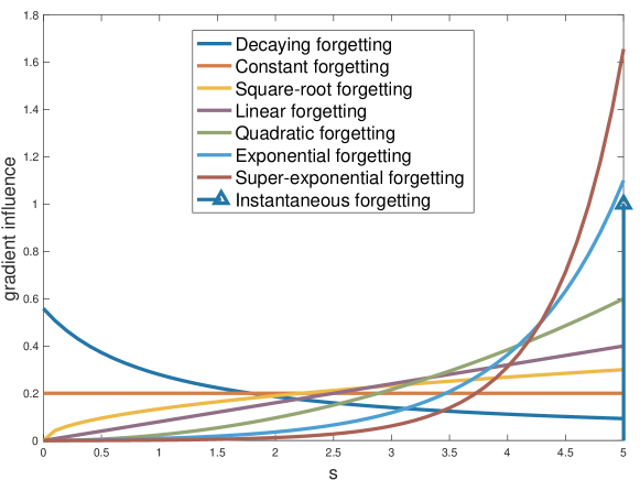
Figure 1: Illustration of the influence of past gradients on $\dot{X}(6)$ (i.e. the right hand side of equation MG-ODE-INT with $t=5$). The corresponding memory function can be found in Tb. 2. The influence is computed as $\dot{\mathfrak{m}}(s)/{\mathfrak{m}}(6)$. By Lemma 3.1, the area under all curves is 1.

Forgetting	Memory $\boldsymbol{{\mathfrak{m}}}$	ODE Coeff. $\boldsymbol{\dot{\mathfrak{m}}/{\mathfrak{m}}}$
Decaying	$\log(1+t)$	$1/(t\log(t+1))$
Constant	$t$	$1/t$
Square-root	$t^{1.5}$	$1.5/t$
Linear	$t^{2}$	$2/t$
Quadratic	$t^{3}$	$3/t$
Exponential	$e^{\alpha t}-1$	$\alpha e^{\alpha t}/\left(e^{\alpha t}-1\right)$
Super-exp	$e^{t^{\alpha}}-1$	$\alpha t^{\alpha-1}e^{t^{\alpha}}/\left(e^{t^{\alpha}}-1\right)$
Instantaneous	$-$	$-$

Table 2: Some important examples of memory functions.

Equivalently, we can transform this second order ODE into a system of two first order ODEs by introducing the variable $V(t):=\dot{X}(t)$ and noting that $\dot{V}(t)=-\frac{\dot{\mathfrak{m}}(t)}{{\mathfrak{m}}(t)}V(t)-\frac{\dot{\mathfrak{m}}(t)}{{\mathfrak{m}}(t)}\nabla f(X(t))$. This is called the phase-space representation of MG-ODE, which we use in Sec. 3.2 to provide the extension to the stochastic setting. Also, for the sake of comparison with recent literature (e.g. [Wibisono et al., 2016]), we provide a variational interpretation of MG-ODE in App. C.2.

Existence and uniqueness.

Readers familiar with ODE theory probably realized that, since by definition ${\mathfrak{m}}(0)=0$, the question of existence and uniqueness of the solution to MG-ODE is not trivial. This is why we stressed its validity for $t>0$ multiple times during the derivation. Indeed, it turns out that such a solution may not exist globally on $[0,\infty)$ (see App. C.1). Nevertheless, if we allow to start integration from any $\epsilon>0$ and assume $f(\cdot)$ to be $L$-smooth, standard ODE theory [Khalil and Grizzle, 2002] ensures that the sought solution exists and is unique on $[\epsilon,\infty)$. Since $\epsilon$ can be made as small as we like (in our simulations in App. F we use $\epsilon=10^{-16}$) this apparent issue can be regarded an artifact of the model. Also, we point out that the integral formulation MG-ODE-INT is well defined for every $t>0$. Therefore, in the theoretical part of this work, we act as if integration starts at $0$ but we highlight in the appendix that choosing the initial condition $\epsilon>0$ induces only a negligible difference (see Remarks C.2 and D.1).

3.2 INTRODUCING STOCHASTIC GRADIENTS

In this section we introduce stochasticity in the MG-ODE model. As already mentioned in the introduction, at each step $k$, iterative stochastic optimization methods have access to an estimate $\mathcal{G}(x_{k})$ of $\nabla f(x_{k})$: the so called stochastic gradient. This information is used and possibly combined with previous gradient estimates $\mathcal{G}(x_{0}),\dots,\mathcal{G}(x_{k-1})$, to compute a new approximation $x_{k+1}$ to the solution $x^{*}$. There are many ways to design $\mathcal{G}(k)$: the simplest [Robbins and Monro, 1951] is to take $\mathcal{G}_{\text{MB}}(x_{k}):=\nabla f_{i_{k}}(x_{k})$, where $i_{k}\in\{1,\dots,n\}$ is a uniformly sampled datapoint. This gradient estimator is trivially unbiased (conditioned on past iterates) and we denote its covariance matrix at point $x$ by $\Sigma(x)=\frac{1}{n}\sum_{i=1}^{n}(\nabla f_{i}(x)-\nabla f(x))(\nabla f_{i}(x)-\nabla f(x))^{T}$.

Following [Krichene and Bartlett, 2017] we model such stochasticity adding a volatility term in MG-ODE.

where $\sigma(X(t))\in{\mathbb{R}}^{d\times d}$ and $\{B(t)\}_{t\geq 0}$ is a standard Brownian Motion. Notice that this system of equations reduces to the phase-space representation of MG-ODE if $\sigma(X(t))$ is the null matrix. The connection from $\sigma(x)$ to the gradient estimator covariance matrix $\Sigma(x)$ can be made precise: [Li et al., 2017] motivate the choice $\sigma(x)=\sqrt{h\Sigma(x)}$, where $\sqrt{\cdot}$ denotes the principal square root and $h$ is the discretization stepsize.

The proof of existence and uniqueness to the solution of this SDE relies on the same arguments made for MG-ODE in Sec. 3.1, with one additional crucial difference: [Orvieto and Lucchi, 2018] showed that $f(\cdot)$ needs to additionally be three times continuously differentiable with bounded third derivative (i.e. $f\in{\mathcal{C}}^{3}_{b}({\mathbb{R}}^{d},{\mathbb{R}})$), in order for $\sigma(\cdot)$ to be Lipschitz continuous. Hence, we will assume this regularity and refer the reader to [Orvieto and Lucchi, 2018] for further details.

3.3 THE CONNECTION TO NESTEROV’S SDE

[Su et al., 2016] showed that the continuous-time limit of NAG for convex functions is HB-ODE with time-dependent viscosity $3/t$: $\ddot{X}(t)+\frac{3}{t}\dot{X}(t)+\nabla f(X(t))=0$, which we refer to as Nesterov’s ODE. Using Bessel functions, the authors were able to provide a new insightful description and analysis of this mysterious algorithm. In particular, they motivated how the vanishing viscosity is essential for acceleration. Indeed, the solution to the equation above is s.t. $f(X(t))-f(x^{*})\leq\mathcal{O}(1/t^{2})$; in contrast to the solution to the GD-ODE $\dot{X}(t)=-\nabla f(X(t))$, which only achieves a rate $\mathcal{O}(1/t)$.

A closer look at Tb. 2 reveals that the choice $3/t$ is related to MG-ODE with quadratic forgetting, that is $\ddot{X}(t)+\frac{3}{t}\dot{X}(t)+\frac{3}{t}\nabla f(X(t))=0$. However, it is necessary to note that in MG-SDE also the gradient term is premultiplied by $3/t$. Here we analyse the effects of this intriguing difference and its connection to acceleration.

Gradient amplification.

A naïve way to speed up the convergence of the GD-ODE $\dot{X}(t)=-\nabla f(X(t))$ is to consider $\dot{X}(t)=-t\nabla f(X(t))$. This can be seen by means of the Lyapunov function $\mathcal{E}(x,t)=t^{2}(f(x)-f(x^{*}))+\|x-x^{*}\|^{2}$. Using convexity of $f(\cdot)$, we have $\dot{\mathcal{E}}(X(t),t)=-t^{2}\|\nabla f(X(t))\|^{2}\leq 0$ and therefore, the solution is s.t. $f(X(t))-f(x^{*})\leq\mathcal{O}(1/t^{2})$. However, the Euler discretization of this ODE is the gradient-descent-like recursion $x_{k+1}=x_{k}-\eta k\nabla f(x_{k})$ — which is not accelerated. Indeed, this gradient amplification by a factor of $t$ is effectively changing the Lipschitz constant of the gradient field from $L$ to $kL$. Therefore, each step is going to yield a descent only if $\eta\leq\frac{1}{kL}$. Yet, this iteration dependent learning rate effectively cancels out the gradient amplification, which brings us back to the standard convergence rate $\mathcal{O}(1/k)$. It is thus natural to ask: "Is the mechanism of acceleration behind Nesterov’s ODE related to a similar gradient amplification?"

In App. C.4 we show that $\{X_{N}(t),V_{N}(t)\}_{t\geq 0}$, the solution to Nesterov’s SDE, is s.t. the infinitesimal update direction $V_{N}(t)$ of the position $X_{N}(t)$ can be written as

$$V_{N}(t)=-\int_{0}^{t}\frac{s^{3}}{t^{3}}\nabla f(X(s))ds+\zeta_{N}(t),$$ (2)

where $\zeta_{N}(t)$ is a random vector with ${\mathbb{E}}[\zeta_{N}(t)]=0$ and $\operatorname{Cov}[\zeta_{N}(t)]=\frac{1}{7}t\sigma\sigma^{T}$. In contrast, the solution $\{X_{{\mathfrak{m}}2}(t),V_{{\mathfrak{m}}2}(t)\})_{t\geq 0}$ of MG-SDE with quadratic forgetting satisfies

$$V_{{\mathfrak{m}}2}(t)=-\int_{0}^{t}\frac{3s^{2}}{t^{3}}\nabla f(X(s))ds+\zeta_{{\mathfrak{m}}2}(t),$$ (3)

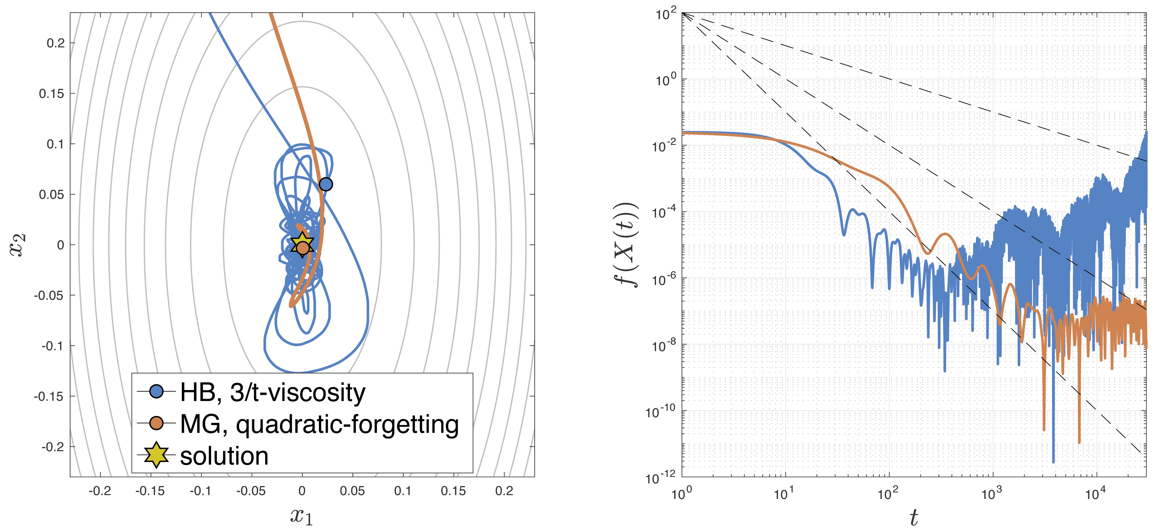
Figure 2: HB-SDE with $\alpha(t)=3/t$ (i.e. Nesterov’s SDE) compared to MG-SDE with quadratic forgetting. Setting as in [Su et al., 2016]: $f(x)=2\times 10^{-2}x_{1}^{2}+5\times 10^{-3}x_{2}^{2}$ starting from $X_{0}=(1,1)$ and $\dot{X}(0)=(0,0)$. Both systems are exposed to the same noise volatility. Simulation using the Milstein scheme [Mil’shtejn, 1975] with stepsize $10^{-3}$.

where $\zeta_{{\mathfrak{m}}2}(t)$ is a random vector with ${\mathbb{E}}[\zeta_{{\mathfrak{m}}2}(t)]=0$ but $\operatorname{Cov}[\zeta_{{\mathfrak{m}}2}(t)]=\frac{9}{5t}\sigma\sigma^{T}$. Even though the reader might already have spotted an important difference in the noise covariances, to make our connection to gradient amplification even clearer, we consider the simpler setting of constant gradients: in this case, we have $V_{N}(t)=-\frac{1}{4}t\nabla f(X(t))+\zeta_{N}(t)$, $V_{{\mathfrak{m}}2}(t)=-\nabla f(X(t))+\zeta_{{\mathfrak{m}}2}(t)$. That is, stochastic algorithms with increasing momentum (i.e. decreasing viscosity, like the Nesterov’s SDE) are systematically amplifying the gradients over time. Yet, at the same time they also linearly amplify the noise variance (see Fig. 7 in the appendix). This argument can easily be extended to the non-constant gradient case by noticing that ${\mathbb{E}}[V_{{\mathfrak{m}}2}(t)]$ is a weighted average of gradients where the weights integrate to 1 for all $t\geq 0$ (Lemma 3.1) . In contrast, in ${\mathbb{E}}[V_{N}(t)]$ these weights integrate to $t/4$. This behaviour is illustrated in Fig. 2: While the Nesterov’s SDE is faster compared to MG-SDE with ${\mathfrak{m}}(t)=t^{3}$ at the beginning, it quickly becomes unstable because of the increasing noise in velocity and hence position.

This gives multiple insights on the behavior of Nesterov’s accelerated method for convex functions, both in for deterministic and the stochastic gradients:

1. Deterministic gradients get linearly amplified overtime, which counteracts the slow-down induced by the vanishing gradient problem around the solution. Interestingly Eq. (2) reveals that this amplification is not performed directly on the local gradient but on past history, with cubic forgetting. It is this feature that makes the discretization stable compared to the naïve approach $\dot{X}=-t\nabla f(X(t))$.

2. Stochasticity corrupts the gradient amplification by an increasing noise variance (see Eq. (2)), which makes Nesterov’s SDE unstable and hence not converging. This finding is in line with [Allen-Zhu, 2017].

Furthermore, our analysis also gives an intuition as to why a constant momentum cannot yield acceleration. Indeed, we saw already that HB-ODE-INT-C does not allow such persistent amplification, but at most a constant amplification inversely proportional to the (constant) viscosity. Yet, as we are going to see in Sec. 4, this feature makes the algorithm more stable under stochastic gradients.

To conclude, we point the reader to App. C.4.2, where we extend the last discussion from the constant gradient case to the quadratic cost case and get a close form for the (exploding) covariance of Nesterov’s SDE (which backs up theoretically the unstable behavior shown in Fig. 2). Nonetheless, we remind that this analysis still relies on continuous-time models; hence, the results above can only be considered as insights and further investigation is needed to translate them to the actual NAG algorithm.

Time warping of linear memory.

Next, we now turn our attention to the following question: "How is the gradient amplification mechanism of NAG related to its — notoriously wiggling— path?". Even though Nesterov’s ODE and MG-ODE with quadratic forgetting are described by similar formulas, we see in Fig. 2 that the trajectories are very different, even when the gradients are large. The object of this paragraph is to show that Nesterov’s path has a strong link to — surprisingly — linear forgetting. Consider speeding-up the linear forgetting ODE $\ddot{X}(t)+\frac{2}{t}\dot{X}(t)+\frac{2}{t}\nabla f(X(t))$ by introducing the time change $\tau(t)=t^{2}/8$ and let $Y(t)=X(\tau(t))$ be the accelerated solution to linear forgetting. By the chain rule, we have $\dot{Y}(t)=\dot{\tau}(t)\dot{X}(\tau(t))$ and $\ddot{Y}(t)=\ddot{\tau}(t)\dot{X}(\tau(t))+\dot{\tau}(t)^{2}\ddot{X}(\tau(t))$. It can easily be verified that we recover $\ddot{Y}(t)+\frac{3}{t}\dot{Y}(t)+\nabla f(Y(t))$. However, in the stochastic setting, the behaviour is still quite different: as predicted by the theory, in Fig. 3 we see that — when gradients are large — the trajectory of the two sample paths are almost identical¹¹ (yet, notice that Nesterov moves faster); however, as we approach the solution, Nesterov diverges while linear forgetting stably proceeds towards the minimizer along the Nesterov’s ODE path, but at a different speed, until convergence to a neighborhood of the solution, as proved in Sec. 4. Furthermore, in App. C.3 we prove that there are no other time changes which can cast MG-ODE into HB-ODE, which yields the following interesting conclusion: the only way to translate a memory system into a momentum method is by using a time change $\tau(t)=\mathcal{O}(t^{2})$.

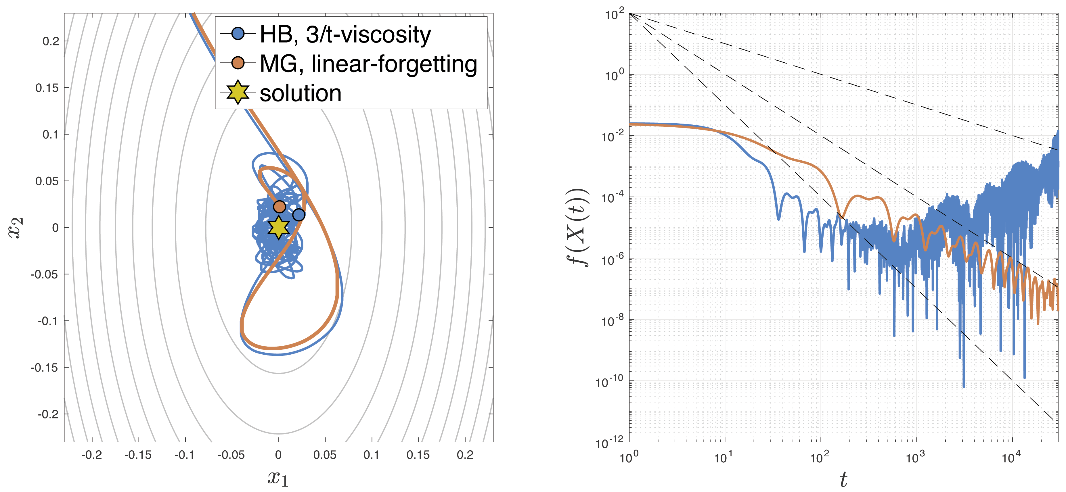
Figure 3: Nesterov’s ODE compared to MG-SDE with linear forgetting (i.e. $\dot{\mathfrak{m}}(t)/{\mathfrak{m}}(t)=2/t$). Same settings as Fig. 2.

Forgetting	Assumption	Rate	Reference
Instantaneous	(H0c), (H1)	${\mathbb{E}}[f(\bar{X}(t))-f(x^{*})]\leq C_{i}/t+\ d\ \sigma^{2}_{*}/2$	[Mertikopoulos and Staudigl, 2018]
Exponential	(H0c), (H1)	${\mathbb{E}}[f(\bar{X}(t))-f(x^{*})]\leq C_{e}/t+\ d\ \sigma^{2}_{*}/2$	App. D, Thm. D.3.1
Polynomial	(H0c), (H1), $p\geq 2$	${\mathbb{E}}[f(X(t))-f(x^{*})]\leq C_{p}/t+p\ d\ \sigma^{2}_{*}/2$	App. D, Thm. D.2

Table 3: Rates of MG-SDE on convex smooth functions . $\bar{X}(t)=\int_{0}^{t}X(s)ds$ and $C_{i},C_{e},C_{p}$ can be found in the references.

4 ANALYSIS AND DISCRETIZATION

In this section we first analyze the convergence properties of MG-SDE under different memory functions. Next, we use the Lyapunov analysis carried out in continuous-time to derive an iterative discrete-time method which implements polynomial forgetting and has provable convergence guarantees. We state a few assumptions:

(H0c) $f\in{\mathcal{C}}^{3}_{b}({\mathbb{R}}^{d},{\mathbb{R}}),\ \sigma_{*}^{2}:=\sup_{x}\|\sigma(x)\sigma(x)^{T}\|_{s}<\infty$.

The definition of $\sigma_{*}^{2}$ nicely decouples the measure of noise magnitude to the problem dimension $d$ (which will then, of course, appear explicitly in all our rates).

(H1)   The cost $f(\cdot)$ is $L$-smooth and convex.

(H2)   The cost $f(\cdot)$ is $L$-smooth and $\mu$-strongly convex.

We provide the proofs (under the less restrictive assumptions of weak-quasi-convexity and quadratic growth), as well as an introduction to stochastic calculus, in App. D.

4.1 EXPONENTIAL FORGETTING

If ${\mathfrak{m}}(t)=e^{\alpha t}-1$, then $\dot{\mathfrak{m}}(t)/{\mathfrak{m}}(t)=\frac{\alpha e^{\alpha t}}{e^{\alpha t}-1}$ which converges to $\alpha$ exponentially fast. To simplify the analysis and for comparison with the literature on HB-SDE (which is usually analyzed under constant volatility [Shi et al., 2018]) we consider here MG-SDE with the approximation $\dot{\mathfrak{m}}(t)/{\mathfrak{m}}(t)\simeq\alpha$. In App. D we show that, under (H1), the rate of convergence of $f(\cdot)$, evaluated at the Cesàro average $\bar{X}(t)=\int_{0}^{t}X(s)ds$ is sublinear (see Tb. 3) to a ball around $x^{*}$ of size $d\ \sigma^{2}_{*}/2$, which is in line with known results for SGD [Bottou et al., 2018]. Note that the size of this ball would change if we were to study a stochastic version of HB-ODE with constant volatility (i.e. $\ddot{X}+\alpha\dot{X}+\nabla f(X)$). In particular, it would depend on the normalization constant in Eq. (1). Also, in App. D, under (H2), we provide a linear convergence rate of the form $f(X(t))-f(x^{*})\leq\mathcal{O}(e^{-\gamma t})$ to a ball ($\gamma$ depends on $\mu$ and $\alpha$). Our result generalizes the analysis in [Shi et al., 2018] to work with any viscosity and with stochastic gradients.

Discretization.

As shown in Sec. 3.1, the discrete equivalent of MG-SDE with exponential forgetting is Adam without adaptive stepsizes (see App. B.2). As for the continuous-time model we just studied, for a sufficiently large iteration, exponential forgetting can be approximated with the following recursive formula:

$$x_{k+1}=x_{k}+\beta(x_{k}-x_{k-1})-\eta(1-\beta)\nabla f(x_{k}),$$

which is exactly HB with learning rate $(1-\beta)\eta$. Hence, the corresponding rates can be derived from Tb. 1.

4.2 POLYNOMIAL FORGETTING

The insights revealed in Sec. 3.3 highlight the importance of the choice ${\mathfrak{m}}(t)=t^{p}$ in this paper. In contrast to instantaneous [Mertikopoulos and Staudigl, 2018] and exponential forgetting, the rate we prove in App. D for this case under (H1) does not involve a Cesàro average — but holds for the last time point (see Tb. 3). This stability property is directly linked to our discussion in Sec. 3.3 and shows that different types of memory may react to noise very differently. Also, we note that the size of the ball we found is now also proportional to $p$; this is not surprising since, as the memory becomes more focused on recent past, we get back to the discussion in the previous subsection and we need to consider a Cesàro average.

Discretization.

Finally, we consider the burning question "Is it possible to discretize MG-SDE — with polynomial forgetting — to derive a cheap iterative algorithm with similar properties?". In App. E, we build this algorithm in a non-standard way: we reverse-engineer the proof of the rate for MG-SDE to get a method which is able to mimic each step of the proof. Starting from $x_{-1}=x_{0}$, it is described by the following recursion

As a direct result of our derivation, we show in Thm. E (App. E) that this algorithm preserves exactly the rate of its continuous-time model in the stochastic setting:

$${\mathbb{E}}[f(x_{k})-f(x^{*})]\leq\frac{(p-1)^{2}\|x_{0}-x^{*}\|^{2}}{2\eta p(k+p-1)}+\frac{1}{2}pd\eta\varsigma_{*}^{2}.$$

We also show that MemSGD-p can be written as $x_{k+1}=x_{k}-\eta\sum_{j=0}^{k}w(j,k)\nabla f(x_{k})$, where $\sum_{j=0}^{k}w(j,k)=1$ (in analogy to the bias correction in Adam) and with $w(\cdot,k)$ increasing as a polynomial of order $p-1$ for all $k$, again in complete analogy with the model. Fig. 4 shows the behaviour of different types of memory in a simple convex setting; as predicted, polynomial (in this case linear) forgetting has a much smoother trajectory then both exponential and instantaneous forgetting. Also, the reader can verify that the asymptotic noise level for MemSGD (p=2) is slightly higher, as just discussed.

For ease of comparison with polynomial memory, we will often write MemSGD (p=e) to denote exponential forgetting (i.e. Adam without adaptive steps) and SGD (p=inf) to stress that SGD implements instantaneous forgetting.

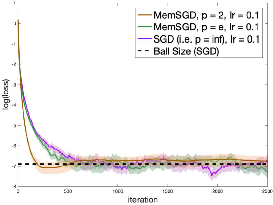
Figure 4: Synthetic example: $f(x_{1},x_{2})=0.8\times x_{1}^{4}+0.4\times x_{2}^{4}$ with Gaussian noise. Displayed is linear forgetting (i.e. MemSGD-2), exponential forgetting (denoted p=e) with $\beta=0.8$ and instantaneous forgetting. Average and 95% confidence interval for 150 runs starting from $(1,1)$.

5 LARGE SCALE EXPERIMENTS

In order to assess the effect of different types of memory in practical settings, we benchmark MemSGD with different memory functions: from instantaneous to exponential, including various types of polynomial forgetting. As a reference point, we also run vanilla HB with constant momentum as stated in the introduction. To get a broad overview of the performance of each method, we run experiments on a convex logistic regression loss as well as on non-convex neural networks in both a mini- and full-batch setting. Details regarding algorithms, datasets and architectures can be found in App. G.1.

Covtype Logreg MNIST Autoencoder FashionMNIST MLP CIFAR-10 CNN  

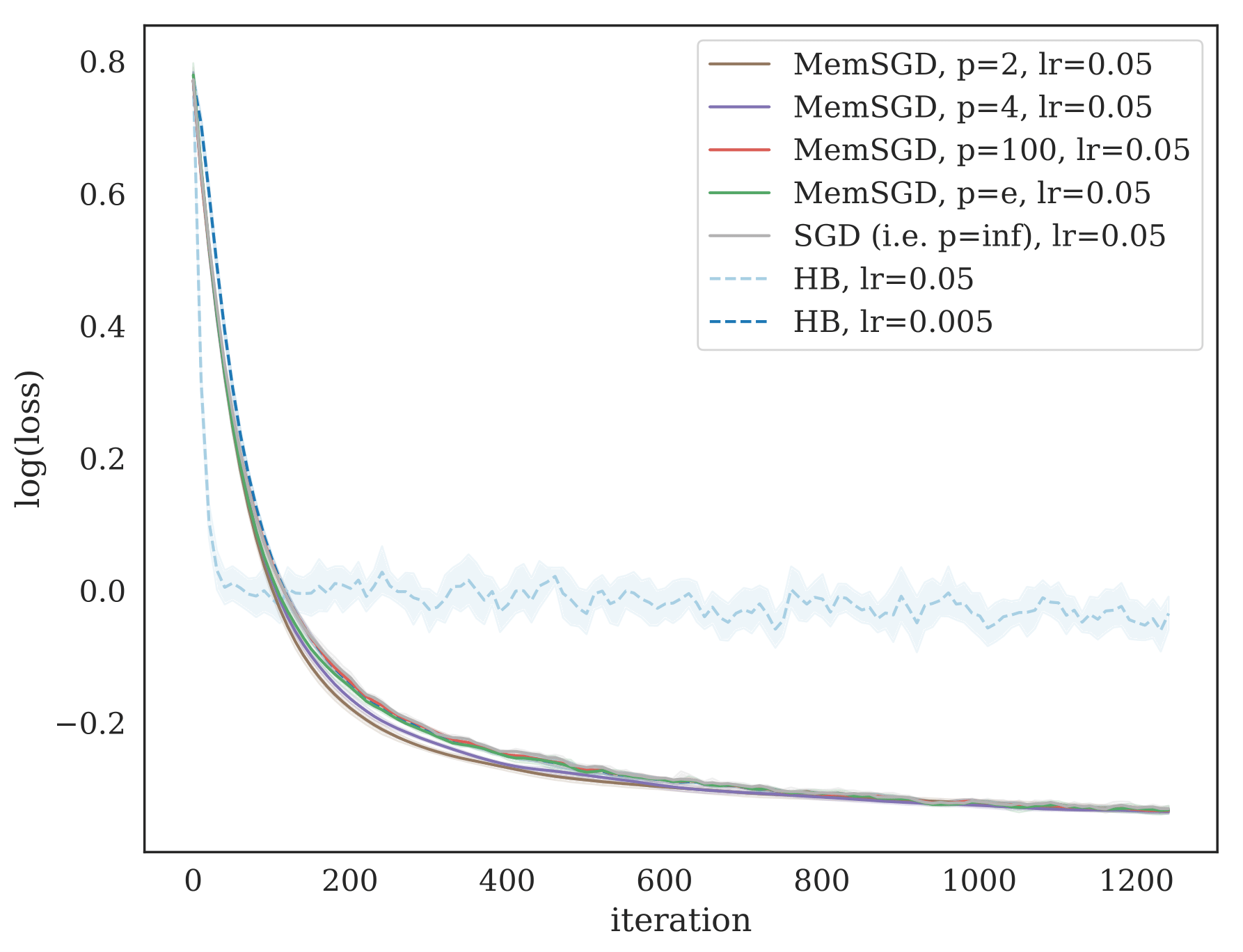
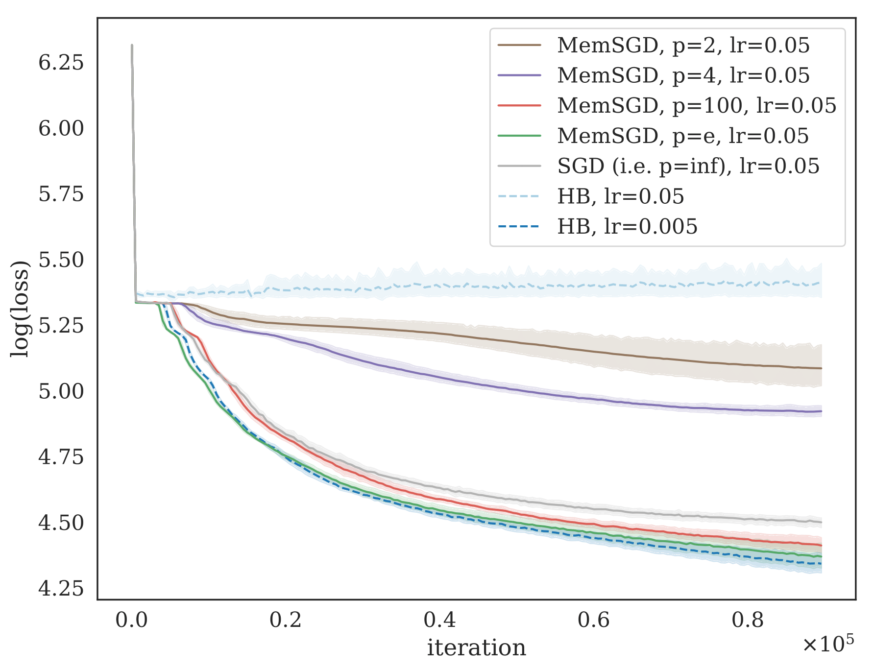
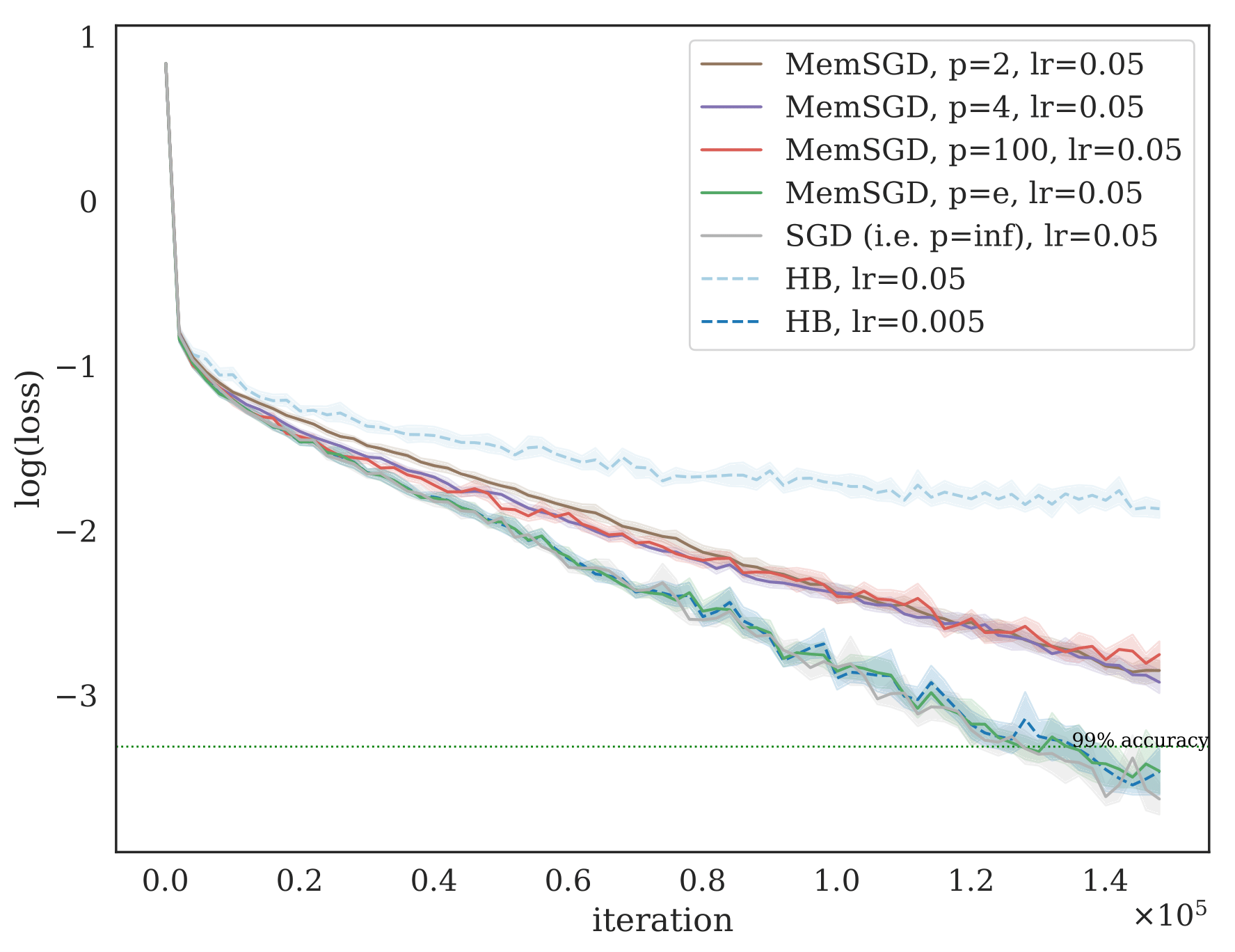
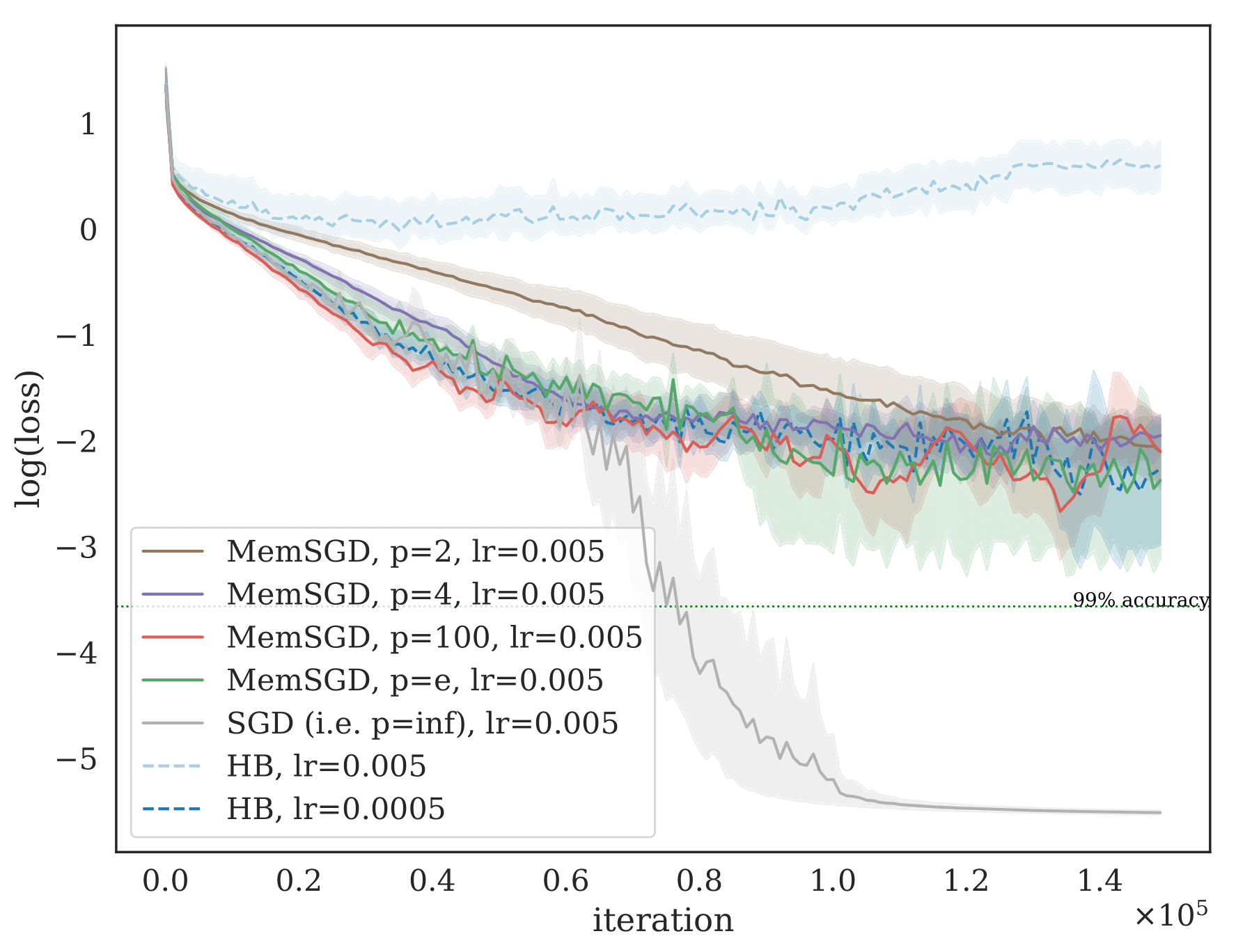
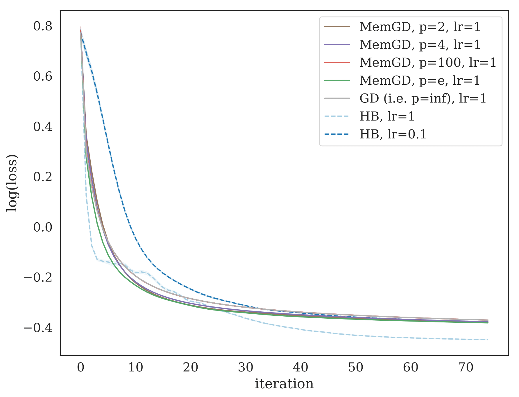
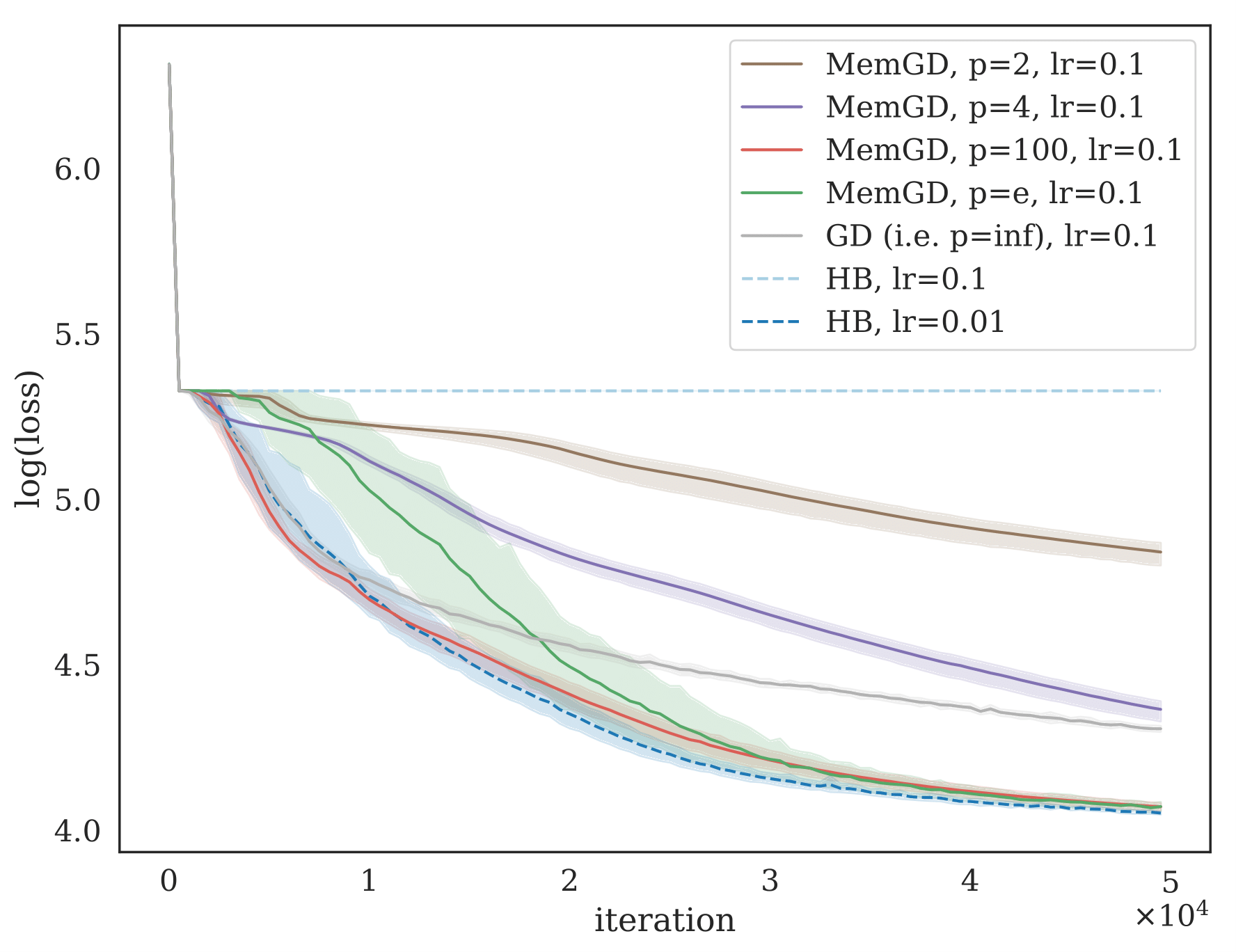
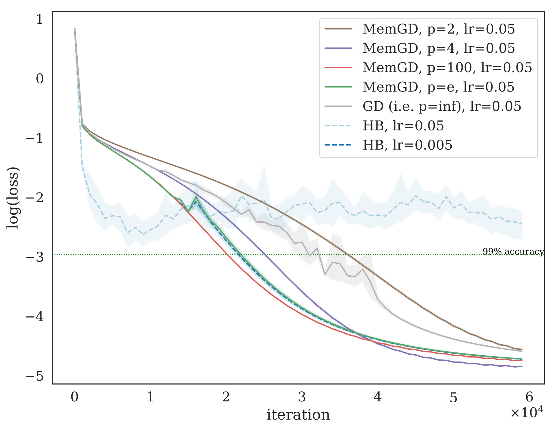
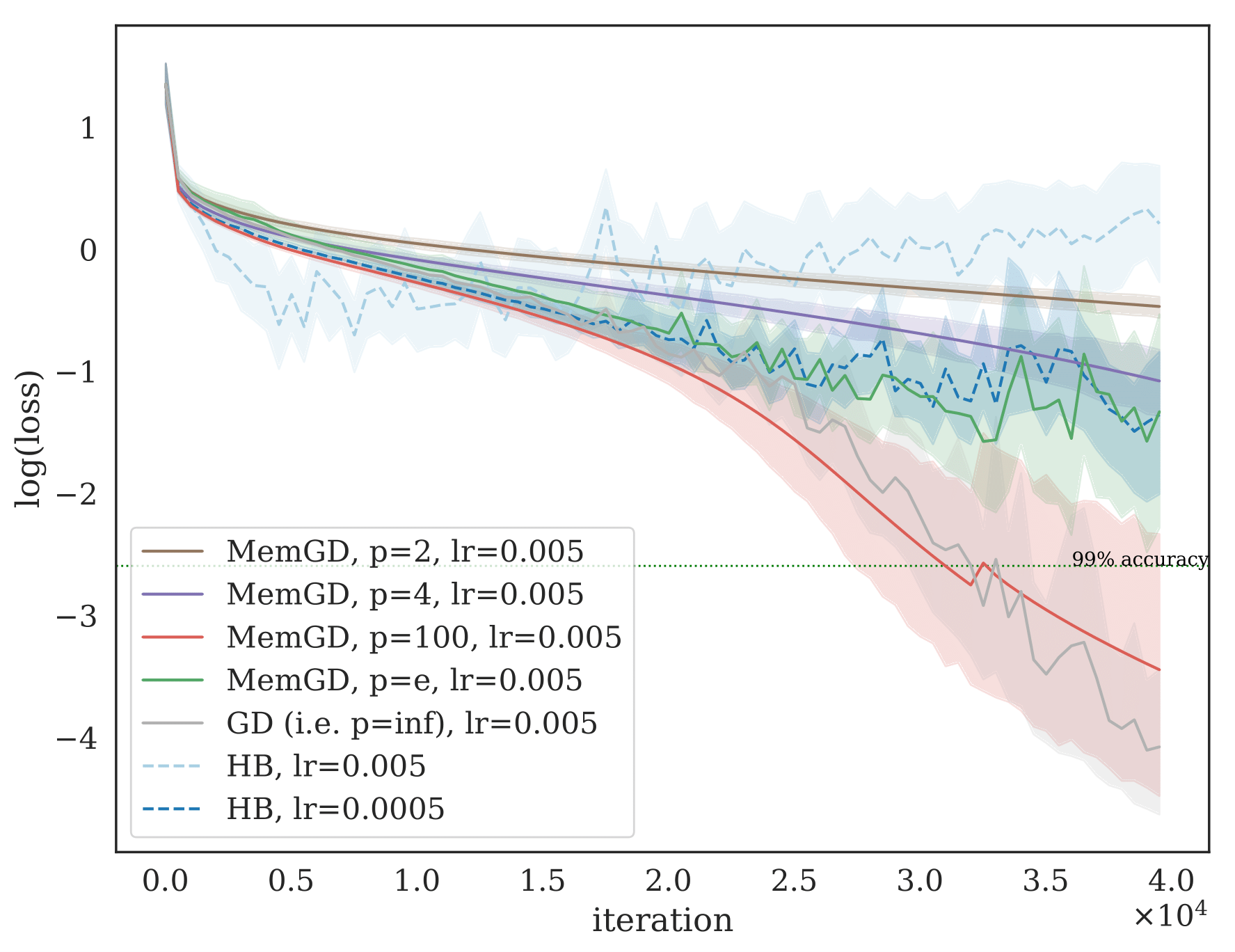
Figure 5: Log loss over iterations in mini- (top) and full-batch (bottom) setting. Average and $95\%$ CI of 10 random initializations.

Results and discussion.

Fig. 5 summarizes our results in terms of training loss. While it becomes evident that no method is best on all problems, we can nevertheless draw some interesting conclusions.

First, we observe that while long-term memory (especially $p=2$) is faster than SGD in the convex case, it does not provide any empirical gain in the neural network settings. This is not particularly surprising since past gradients may quickly become outdated in non-convex landscapes. Short term memory is at least as good as SGD in all cases except for the CIFAR-10 CNN, which represents the most complex of our loss landscapes in terms of curvature.

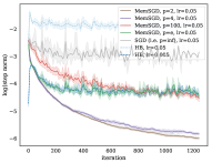
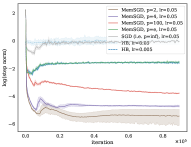
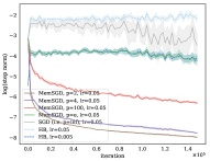
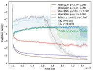
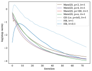
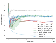
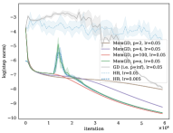
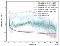
Figure 15: Real world experiments: Log step norm over iterations in mini- (top) and full batch (bottom) setting. Average and $95\%$ confidence interval of 10 runs with random initialization.

Secondly, we find that the best stepsize for HB is always strictly smaller than the one for SGD in the non-convex setting. MemSGD, on the other hand, can run on stepsizes as large as SGD which reflects the gradient amplification of HB as well as the unbiasedness of MemSGD. Interestingly, however, a closer look at Fig. 15 (appendix) reveals that HB (with best stepsize) actually takes much smaller steps than SGD for almost all iterations. While this makes sense from the perspective that memory averages past gradients, it is somewhat counter-intuitive given the inertia interpretation of HB which should make the method travel further than SGD. Indeed, both [Sutskever et al., 2013] and [Goodfellow et al., 2016] attribute the effectiveness of HB to its increased velocity along consistent directions (especially early on in the optimization process). However, our observation, together with the fact that MemSGD with fast forgetting ($p=e$ and $p=100$) is as good as HB, suggests that there is actually more to the success of taking past gradients into account and that this must lie in the altered directions that adapt better to the underlying geometry of the problem.

Finally, we draw two conclusions that arise when comparing the mini- and full batch setting. First, the superiority of HB and fast forgetting MemSGD over vanilla SGD in the deterministic setting is indeed reduced as soon as stochastic gradients come into play (this is in line with the discussion in Sec. 3.3). Second, we find that stochasticity per se is not needed to optimize the neural networks in the sense that all methods eventually reach very similar methods of suboptimality. That is, not even the full batch methods get stuck in any elevated local minima including the saddle found in the MNIST autoencoder which they nicely escape (given the right stepsize).

6 MEMORY IN ADAPTIVE METHODS

While the main focus of this paper is the study of the effect of different types of memory on the first moment of the gradients, past gradient information is also commonly used to adapt stepsizes. This is the case for Adagrad and Adam which both make use of the second moment of past gradients to precondition their respective update steps.

Of course, the use of polynomial memory generalizes directly to the second moment estimates and we thus consider a comprehensive study of the effect of long- versus short-term memory in adaptive preconditioning an exciting direction of future research. In fact, as shown in [Reddi et al., 2018] the non-convergence issue of Adam can be fixed by making the method forget past gradients less quickly. For that purpose the authors propose an algorithm called AdamNC that essentially differs from Adam by the choice of $\beta_{2}=1-1/k$, which closely resembles Adagrad with constant memory. Interestingly, the memory framework introduced in this paper allows to interpolate between the two extremes of constant- and exponential memory (i.e. Adagrad and Adam) in a principled way. Indeed, by tuning the additional parameter $p$ — which specifies the degree of the polynomial memory function — one can equip Adam with any degree of short- to long-term memory desired. As a proof of concept, Fig. 6 shows that Adam equipped with a polynomial memory of the squared gradients (PolyAdam) can in fact be faster than both Adam and Adagrad.

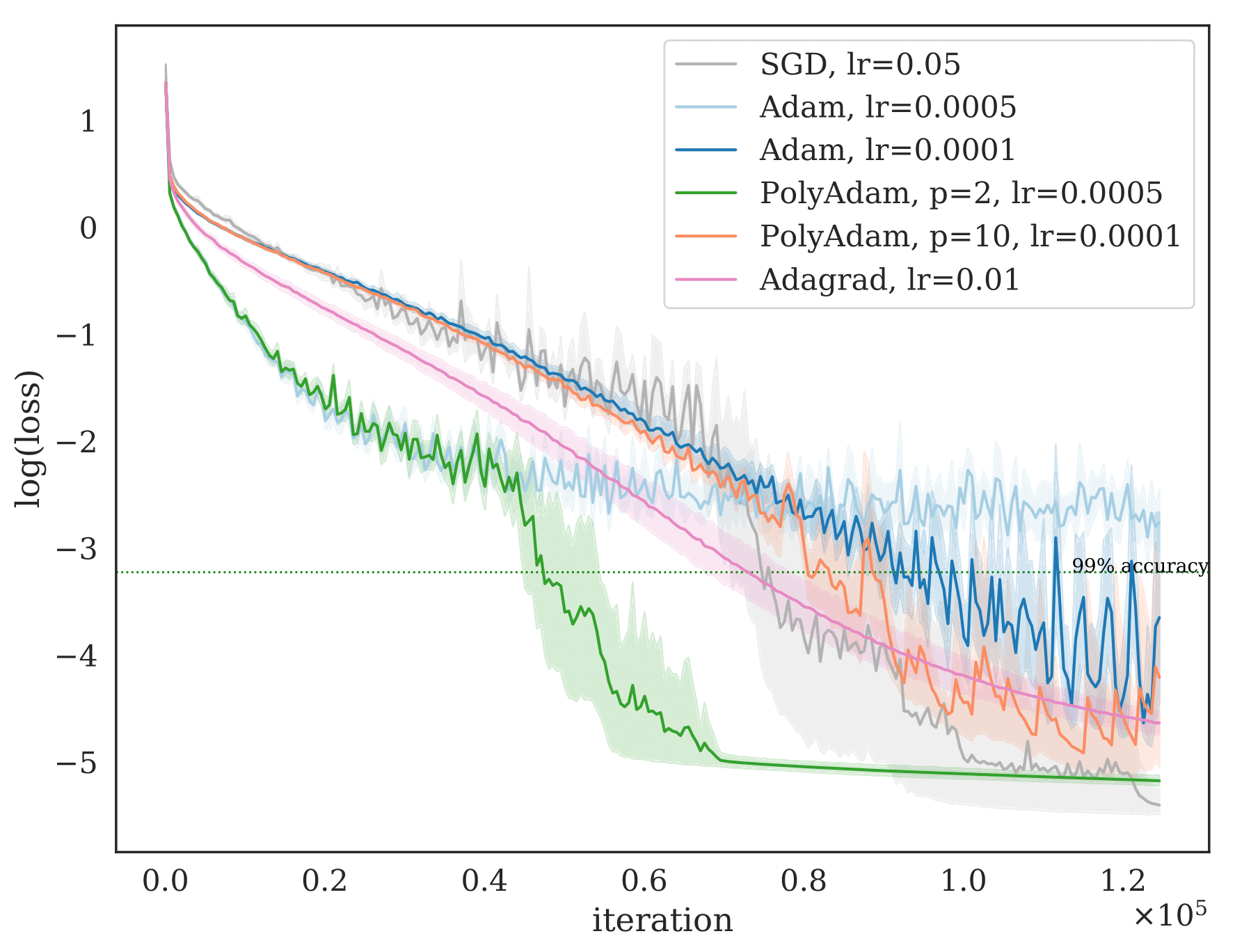
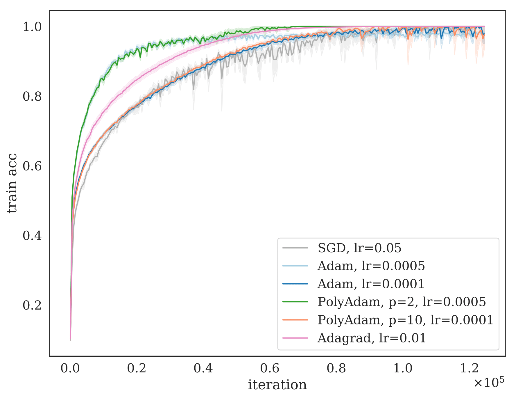
Figure 6: Cifar-10 CNN: Log loss over iterations (left) and training accuracy (right). Average and $95\%$ confidence interval of 10 runs with random initialization.

7 CONCLUSION

We undertook an extensive theoretical study of the role of memory in (stochastic) optimization. We provided convergence guarantees for memory systems as well as for novel algorithms based on such systems. This study led us to derive novel insights on momentum methods. We complemented these findings with empirical results, both on simple functions as well as more complex functions based on neural networks. There, long- and short-term memory methods exhibit a different behaviour, which suggests further investigation is needed to better understand the interplay between the geometry of neural networks losses, memory and gradient stochasticity. On a more theoretical side, an interesting direction of future work is the study of the role of memory in state-of-the art momentum methods such as algorithms that include primal averaging, increasing gradient sensitivity or decreasing learning rates (see e.g. [Krichene and Bartlett, 2017]).

Appendix

Appendix A Basic Definitions and Notation

In this paper we work in ${\mathbb{R}}^{d}$ with the metric induced by the Euclidean norm, which we denote by $\|\cdot\|$. We say that $f:{\mathbb{R}}^{d}\to{\mathbb{R}}$ is ${\mathcal{C}}^{m}({\mathbb{R}}^{d},{\mathbb{R}})$ if it is $m$ times continuously differentiable and we say that it is $L$-Lipschitz if $\|\nabla f(x)-\nabla f(y)\|\leq L\|x-y\|$ for all $x,y\in{\mathbb{R}}^{d}$. We say that $f(\cdot)$ is $\mu$-strongly convex if $f(y)\geq f(x)+\langle\nabla f(x),y-x\rangle+\frac{\mu}{2}\|y-x\|^{2}$ for all $x,y\in{\mathbb{R}}^{n}$. We call a function convex if it is $0$-strongly convex. An equivalent definition involves the Hessian: a twice differentiable function $f(\cdot)$ is $\mu$-strongly convex and $L$-smooth if and only if, for all $x\in{\mathbb{R}}^{d}$ , $\mu I_{d}\preceq\|\nabla^{2}f(x)\|_{s}\preceq LI_{d}$, where $I_{d}$ is the identity matrix in ${\mathbb{R}}^{d}$ and $\|\cdot\|_{s}$ denotes the operator norm of a matrix in Euclidean space: $\|\nabla^{2}f(x)\|_{s}=\sup_{\|y\|=1}\|\nabla^{2}f(x)y\|$. For a symmetric matrix, the operator norm is the norm of the maximum positive eigenvalue.

Appendix B Background on Momentum and Adam

All the algorithms/ODEs mentioned in this appendix are reported in Sec. 3.

B.1 Discretization of HB-ODE

The next theorem provides a strong link between HB and HB-ODE, and in partially included in [Shi et al., 2019]. The Heavy-Ball is the result of some semi-implicit Euler integration on (HB-ODE-PS).

Proof.

Semi-implicit integration with stepsize $h$, at iteration $k$ and from the current integral approximation $(x_{k},v_{k})\simeq\left(X(kh),V(kh)\right)$, computes $(x_{k+1},v_{k+1})\simeq\left(X(h(k+1)),V(h(k+1))\right)$ as follows:

$$\begin{cases}v_{k+1}=v_{k}+h(-a_{k}v_{k}-\nabla f(x_{k}))\\ x_{k+1}=x_{k}+hv_{k+1}\end{cases},$$ (4)

where $a_{k}=a(hk)$. Notice that $v_{k+1}=\frac{x_{k+1}-x_{k}}{h}$ and

$$x_{k+1}=x_{k}-(1-a_{k}h)(x_{k}-x_{k-1})-h^{2}\nabla f(x_{k}),$$ (5)

which is exactly an Heavy Ball iteration, with $\beta_{k}=1-ha_{k}$ and $\eta=h^{2}$. ∎

Remark B.1.

The semi-implicit Euler method —when applied to an Hamiltonian system— is symplectic, meaning that is preserves some geometric properties of the true solution [Hairer et al., 2006]. However, as also pointed out in [Zhang et al., 2018], continuous time models of momentum methods are energy-dissipative —hence not Hamiltonian. Therefore, as opposed to [Betancourt et al., 2018, Shi et al., 2019], we avoid using this misleading moniker.

Moreover, the last result also has an integral formulation. The differential equation HB-ODE-INT-C is the continuous time limit of HB-SUM.

Proof.

Recalling that $\beta=1-h\alpha$ (where $h$ is the stepsize of the semi-implicit Euler integration defined in Thm. B.1) and choosing $t=kh$ ($k>0$) and $s=jh$ ($j>0$),

$$\lim_{h\to 0}\beta^{k-j}=\lim_{h\to 0}(1-h\alpha)^{(t-s)/h}=\lim_{h\to 0}\left((1-h\alpha)^{1/h}\right)^{(t-s)}=\left(e^{\alpha}\right)^{(t-s)}=e^{\alpha(t-s)}.$$

Moreover, since $\eta=h^{2}$, taking one $h$ inside the summation, we get a Riemann sum which then rightfully converges to the integral in the limit. ∎

B.2 Unbiasing HB-SUM under constant momentum: the birth of Adam

[Kingma and Ba, 2014] noticed that, in the limit case where true gradients are constant, the averaging procedure in HB-SUM (defined in the Introduction section of the main paper) is biased: let $i_{j}\in\{1,\dots,N\}$ be the data-point selected at iteration $j$ and $\nabla f_{i_{j}}$ the corresponding stochastic gradient; if we define $\epsilon_{j}:=\nabla f(x_{j})-\nabla f_{i_{j}}(x_{j})$ and pick constant momentum $\beta_{j}=\beta$, we have

$${\mathbb{E}}\left[\sum_{j=0}^{k}\beta^{k-j}\nabla f_{i_{j}}(x_{j})\right]=\sum_{j=0}^{k}\beta^{k-j}{\mathbb{E}}[\nabla f+\epsilon_{j}]=\frac{\beta^{k+1}-1}{\beta-1}\nabla f.$$

Therefore —to ensure an unbiased update, at least for this simple case— [Kingma and Ba, 2014] normalize the sum above by $\frac{\beta^{k+1}-1}{\beta-1}$, showing significant benefits in the experimental section. Indeed, such normalization retains all the celebrated geometric properties of momentum (see Introduction), while improving statistical accuracy —a crucial feature of SGD. For convenience of the reader, we report below the full Adam algorithm.

In addition, such normalization also performs variance reduction. Indeed, let $\Sigma:=\operatorname{Cov}\left[\nabla f_{i}(x)\right]$ be the gradient covariance, which we assume constant and finite for simplicity. Then,

$$\operatorname{Cov}\left[\frac{\beta-1}{\beta^{k+1}-1}\sum_{j=0}^{k}\beta^{k-j}\nabla f_{i_{j}}(x_{j})\right] =\frac{(\beta-1)^{2}}{(\beta^{k+1}-1)^{2}}\sum_{j=0}^{k}\beta^{2(k-j)}\Sigma$$

$$=\frac{(\beta-1)^{2}}{(\beta^{k+1}-1)^{2}}\frac{\beta^{2(k+1)}-1}{\beta^{2}-1}\Sigma$$

$$=\frac{\beta-1}{(\beta^{k+1}-1)}\frac{\beta^{k+1}+1}{\beta+1}\Sigma\preceq\Sigma.$$

Note that if $k$ increases, the covariance monotonically decreases until reaching the minimum $\frac{1-\beta}{\beta+1}\Sigma$ at infinity. We also note that, in case $\beta=0$ (Gradient Descent) we have no variance reduction, as expected.

Supported by the empirical success of Adam[Kingma and Ba, 2014], we suggest in the main paper to modify the standard Heavy Ball (HB-SUM) with constant momentum to match the Adam update:

$$x_{k+1}=x_{k}-\eta\frac{\beta-1}{\beta^{k+1}-1}\sum_{j=0}^{k}\beta^{k-j}\nabla f(x_{j}).$$ (6)

Which can be written recursively using 3 variables (see again [Kingma and Ba, 2014]). Notice that, after a relatively small number of iterations, we converge to the simpler update rule

$$x_{k+1}=x_{k}+\beta(x_{k}-x_{k-1})-\eta(1-\beta)\nabla f(x_{k}),$$

which is also the starting point in some recent elaboration on Heavy Ball [Ma and Yarats, 2018].

Appendix C Time-warping, acceleration and gradient amplification

C.1 Counterexample for existence of a solution of MG-ODE starting integration at 0

Consider the one dimensional dynamics with gradients always equal to one and ${\mathfrak{m}}(t)=t^{3}$. The MG-ODE (see main paper) reads $\ddot{X}(t)+\frac{3}{t}\dot{X}+\frac{3}{t}=0$. It is easy to realize using a Cauchy-Euler argument that all solutions are of the form $X(t)=\frac{c_{1}}{t^{2}}+c_{2}-t$. Unfortunately, the constraint $X(0)=x_{0}$ fixes both the degrees of freedom and fixes $X(t)=x_{0}-t$, so that we necessarily have $\dot{X}(0)=-1$.

C.2 Variational point of view

Let $X\in{\mathcal{C}}^{1}([t_{1},t_{2}],{\mathbb{R}}^{d})$ be a curve; the action (see [Arnol’d, 2013] for the precise definition) associated with a Lagrangian $\mathcal{L}:{\mathbb{R}}^{d}\times{\mathbb{R}}^{d}\times{\mathbb{R}}\to{\mathbb{R}}$ is $\int_{t_{1}}^{t_{2}}\mathcal{L}(X(s),\dot{X}(s),s)ds$. The fundamental result in variational analysis states that the curve $X$ is a stationary point for the action only if it solves the Euler-Lagrange equation $\frac{d}{dt}\partial_{\dot{X}}\mathcal{L}(X(t),\dot{X}(t),t)=\partial_{X}\mathcal{L}(X(t),\dot{X}(t),t)$. We define the Memory Lagrangian as

$$\boxed{\mathcal{L}_{\mathfrak{m}}(X,\dot{X},t):=\frac{1}{2}{\mathfrak{m}}(t)\|\dot{X}\|^{2}-\dot{\mathfrak{m}}(t)f(X)}.$$

It is straightforward to verify that the associated Euler-Lagrange equations give rise to MG-ODE. We cannot help but noticing the striking simplicity of this Lagrangian when compared to others arising from momentum methods (see e.g. the Bregman Lagrangian in [Wibisono et al., 2016]) . For the sake of delivering other points in this paper, we leave the analysis of the symmetries of $\mathcal{L}_{\mathfrak{m}}$ to future work.

C.3 Time-warping of memory: a general correspondence to HB-ODE

Consider the ODE $\boxed{\ddot{X}(t)+\frac{\dot{\mathfrak{m}}(t)}{{\mathfrak{m}}(t)}\dot{X}(t)+\frac{\dot{\mathfrak{m}}(t)}{{\mathfrak{m}}(t)}\nabla f(X)=0}$ and the time change $\tau(t)$.

Let $Y(t)=X(\tau(t))$, following [Wibisono et al., 2016] we have, by the chain rule,

$$\dot{Y}(t)=\dot{X}(\tau(t))\dot{\tau}(t);\ \ \ \ \ \ \ \ \ddot{Y}(t)=\dot{X}(\tau(t))\ddot{\tau}(t)+(\dot{\tau}(t))^{2}\ddot{X}(\tau(t)).\\$$

Therefore, we have

$$\dot{X}(\tau(t))=\frac{\dot{Y}(t)}{\dot{\tau}(t)};\ \ \ \ \ \ \ \ \ddot{X}(\tau(t))=\frac{\ddot{Y}(t)}{(\dot{\tau}(t))^{2}}-\frac{\ddot{\tau}(t)}{(\dot{\tau}(t))^{3}}\dot{Y}(t).\\$$

Next, we construct a new ODE for $Y$ using the previous formulas:

$$\frac{1}{(\dot{\tau}(t))^{2}}\ddot{Y}(t)+\left(\frac{\dot{\mathfrak{m}}(\tau(t))}{\dot{\tau}(t){\mathfrak{m}}(\tau(t))}-\frac{\ddot{\tau}(t)}{(\dot{\tau}(t))^{3}}\right)\dot{Y}(t)+\frac{\dot{\mathfrak{m}}(\tau(t))}{{\mathfrak{m}}(\tau(t))}\nabla f(X(\tau(t)));$$

Next, we multiply everything by ${\mathfrak{m}}(\tau(t))/\dot{\mathfrak{m}}(\tau(t))$, in order to eliminate the coefficient in front of the gradient:

$$\frac{{\mathfrak{m}}(\tau(t))}{\dot{\mathfrak{m}}(\tau(t))(\dot{\tau}(t))^{2}}\ddot{Y}(t)+\left(\frac{1}{\dot{\tau}(t)}-\frac{{\mathfrak{m}}(\tau(t))\ddot{\tau}(t)}{\dot{\mathfrak{m}}(\tau(t))(\dot{\tau}(t))^{3}}\right)\dot{Y}(t)+\nabla f(Y(t))$$

If we also want the coefficient in front of $\ddot{Y}(t)$ to be one, we need $\tau(t)$ to satisfy the following differential equation:

$${\mathfrak{m}}(\tau(t))=\dot{\mathfrak{m}}(\tau(t))(\tau(t))^{2}.$$

For simplicity, let us consider ${\mathfrak{m}}(t)=t^{p}$, for some $p$ (polynomial forgetting), the equation reduces to $\tau(t)=p(\dot{\tau}(t))^{2}$, which has the general solution

$$\tau(t)=\frac{1}{4p}\left(-2\sqrt{2}c_{1}t+2c_{1}^{2}+t^{2}\right).$$

To be a valid time change, we need to have $\tau(0)=0$; hence, — only one choice is possible: $\tau(t)=\frac{t^{2}}{4p}$. Plugging in this choice into the differential equation, we get

$$\boxed{\ddot{Y}(t)+\frac{2p-1}{t}\dot{Y}(t)+\nabla f(Y(t))=0},$$

which is of the form of HB-ODE.

In all this, it is the time change is fixed to be $\frac{t^{2}}{4p}$. For this reason, we postulate that this time change analysis has deep links to the general mechanism of acceleration. We verify this change of time/ODE formula in App. F.

C.4 Behaviour of Nesterov’s SDE compared to the quadratic forgetting SDE

We compare here the variance of the Nesterov’s SDE to the variance of the quadratic forgetting SDE.

C.4.1 A general result

First, we need to prove a result in stochastic integration (for the definition of integral w.r.t. a Brownian Motion the reader can check [Mao, 2007]).

Let $\{B\}_{t\geq 0}$ be a $d-$dimensional Brownian Motion,

$$\operatorname{Cov}\left(\int_{0}^{t}s^{p}dB(s)\right)=\frac{t^{2p+1}}{2p+1}I_{d}.$$

Proof.

First, notice that ${\mathbb{E}}\left[\int_{0}^{t}s^{p}dB(s)\right]=0$; therefore the variance is equal to the second moment:

$$\operatorname{Cov}\left(\int_{0}^{t}s^{p}dB(s)\right)={\mathbb{E}}\left[\left(\int_{0}^{t}s^{p}dB(s)\right)^{2}\right].$$

By the Itô isometry (see e.g. [Mao, 2007]).

$${\mathbb{E}}\left[\left(\int_{0}^{t}s^{p}dB(s)\right)^{2}\right]=\int_{0}^{t}s^{2p}dt=\frac{t^{2p+1}}{2p+1}.$$

∎

We want to compare the SDEs below.

$$\boxed{\begin{cases}dX(t)=V(t)dt\\ dV(t)=-\frac{3}{t}V(t)dt-\frac{3}{t}\left[\nabla f(X(t))dt+\sigma(X(t))dB(t)\right]\end{cases}}$$ (quadratic forgetting SDE)

$$\boxed{\begin{cases}dX(t)=V(t)dt\\ dV(t)=-\frac{3}{t}V(t)dt-\left[\nabla f(X(t))dt+\sigma(X(t))dB(t)\right]\end{cases}}\ \ \ \ \ \ \ \ \ \ \ \ \ \ \ \ \ \$$ (Nesterov’s SDE)

We have the following result, which is included in Sec. 3.3 of the main paper. Assume persistent volatility $\sigma(X(t))=\sigma$. Let $\{X_{N}(t),V_{N}(t)\}_{t\geq 0}$ be the stochastic process which solves Nesterov’s SDE. The infinitesimal update direction $V_{N}(t)$ of the position $X_{N}(t)$ can be written as

$$V_{N}(t)=-\int_{0}^{t}\frac{s^{3}}{t^{3}}\nabla f(X_{N}(s))ds+\zeta_{N}(t),$$

where $\zeta_{N}(t)$ is a random vector with ${\mathbb{E}}[\zeta_{N}(t)]=0$ and $\operatorname{Cov}[\zeta_{N}(t)]=\frac{1}{7}t\sigma\sigma^{T}$. In contrast, the solution $\{X_{{\mathfrak{m}}2}(t),V_{{\mathfrak{m}}2}(t)\})_{t\geq 0}$ of MG-SDE with quadratic forgetting satisfies

$$V_{{\mathfrak{m}}2}(t)=-\int_{0}^{t}\frac{3s^{2}}{t^{3}}\nabla f(X_{{\mathfrak{m}}2}(s))ds+\zeta_{{\mathfrak{m}}2}(t),$$

where $\zeta_{{\mathfrak{m}}2}(t)$ is a random vector with ${\mathbb{E}}[\zeta_{{\mathfrak{m}}2}(t)]=0$ but $\operatorname{Cov}[\zeta_{{\mathfrak{m}}2}(t)]=\frac{9}{5t}\sigma\sigma^{T}$.

Remark C.1 (implications of the proposition).

Note that, in the result above, the time integrals themselves are random variables; therefore, in general, $\operatorname{Cov}[V_{{\mathfrak{m}}2}(t)]\neq\operatorname{Cov}[\zeta_{{\mathfrak{m}}2}(t)]$ and $\operatorname{Cov}[V_{N}(t)]\neq\operatorname{Cov}[\zeta_{N}(t)]$. Therefore, the result does not directly imply that $\operatorname{Cov}[V_{N}(t)]$ explodes. However, if gradients are constant, then clearly $\operatorname{Cov}[V_{N}(t)]$ diverges since the integrals are deterministic (see Fig.7). A more careful analysis, presented in App. C.4.2, shows that this fact also holds in the quadratic convex case.

Proof.

Let us consider first the Quadratic forgetting SDE. Define the function $Q(v,t)=t^{3}v$, which has Jacobian $\partial_{v}Q(v,t)=t^{3}I_{d}$. Using Itô’s Lemma (Eq. (11)) coordinate-wise, we get

$$dQ(V(t),t) =\partial_{t}Q(V(t),t)dt+\left\langle\partial_{v}Q(V(t),t),-\frac{3}{t}V(t)dt-\frac{3}{t}\nabla f(X(t))dt\right\rangle+\left\langle\partial_{v}Q(V,t),-\sigma dB(t)\right\rangle$$

$$=\cancel{3t^{2}V(t)dt}-\cancel{3t^{2}V(t)dt}-3t^{2}\nabla f(X(t))dt-3t^{2}\sigma dB(t),$$ (7)

which implies, after taking the stochastic integral,

$$t^{3}V(t)=Q(V(t),t)-Q(V(0),0)=-\int_{0}^{t}3s^{2}\nabla f(X(s))ds-\int_{0}^{t}3s^{2}\sigma dB(s).$$

Therefore, for any $t\geq 0$,

$$V_{2{\mathfrak{m}}}(t)=-\int_{0}^{t}\frac{3s^{2}}{t^{3}}\nabla f(X(s))ds-\int_{0}^{t}\frac{3s^{2}}{t^{3}}\sigma dB(s).$$

Let us call $\zeta_{2{\mathfrak{m}}}(t)$ the stochastic integral, by Lemma C.4.1,

$$\operatorname{Cov}\left[\zeta_{2{\mathfrak{m}}}(t)\right]=\frac{9}{t^{6}}\frac{t^{5}}{5}\sigma\sigma^{T}=\frac{9}{5t}\sigma\sigma^{T}.$$

If we apply the same procedure to Nesterov’s SDE, we instead get

$$V_{N}(t)=-\int_{0}^{t}\frac{s^{3}}{t^{3}}\nabla f(X(s))ds-\int_{0}^{t}\frac{s^{3}}{t^{3}}\sigma dB(s)=-\int_{0}^{t}\frac{s^{3}}{t^{3}}\nabla f(X(s))ds-\zeta_{2{\mathfrak{m}}}(t),$$

where $\operatorname{Cov}\left(\zeta_{2{\mathfrak{m}}}(t)\right)=\frac{t}{7}\sigma\sigma^{T}.$ ∎

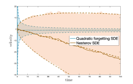
Figure 7: Simulation using Milstein scheme [Mil’shtejn, 1975] (stepsize $10^{-3}$, equivalent for this case to Euler-Maruyama) to verify gradient amplification and covariance explosion under a constant gradient equal to 1, $\sigma=10$. Plotted is the empirical mean and standard deviation of the velocity variable using 1000 runs. The dashed lines indicates the prediction from Prop. C.4.1. MG-SDE with quadratic forgetting quickly settles to the value $-1$ (the true negative gradient) with decreasing variance. Nesterov’s SDE amplifies linearly the negative gradient, and such amplification makes the velocity noisy, with exploding variance.

Remark C.2 (effect of starting integration after 0).

Effect of starting integration after 0. We take the chance here to explain what changes if we start integration at $\epsilon>0$ with $V_{\epsilon}(\epsilon)=0$ and $X_{\epsilon}(\epsilon)=x_{0}$. Starting from Eq. (7), which is still valid, we have to integrate on $[\epsilon,t].$

we have, after taking the stochastic integral,

$$t^{3}V_{\epsilon}(t)-\epsilon^{3}V_{\epsilon}(\epsilon)=-\int_{\epsilon}^{t}3s^{2}\nabla f(X_{\epsilon}(s))ds-\int_{\epsilon}^{t}3s^{2}\sigma dB(s).$$

Notice that $V_{\epsilon}(\epsilon)=0$; therefore

$$V(t)=-\int_{\epsilon}^{t}\frac{3s^{2}}{t^{3}}\nabla f(X(s))ds-\int_{\epsilon}^{t}3s^{2}\sigma dB(s).$$

Notice that, for all $t\geq 0$, the integral dependency on $\epsilon$ vanishes as $\epsilon$ goes to zero. More explicitly, this can be seen using a change of variable in the integral and considering any fixed function $X(s)$.

C.4.2 Variance divergence of Nesterov’s SDE in the quadratic case

Consider $f(x)=\frac{1}{2}\langle x-x^{*},H(x-x^{*})\rangle$ for some positive semidefinite $H$. Without loss of generality, we can assume $H$ to be diagonal and $x^{*}=0_{d}$, the ${\mathbb{R}}^{d}$ vector of all zeros. Then, in the quadratic-forgetting SDE and Nesterov’s SDE, each direction in the original space evolves separately and is decoupled from the others. In other words, the problem becomes linear and two dimensional.

Let us perform the analysis for Nesterov first. We call $\{X_{N}(t),V_{N}(t)\}_{t\geq 0}$, the solution to Nesterov’s SDE and denote by $X_{N}^{i}(t)$ and $V_{N}^{i}(t)$ the i-th coordinates of the space and velocity variables and by $\lambda_{i}\in{\mathbb{R}}_{+}$ the eigenvalue of $H$ in the i-th eigendirection. We want to show that ${\mathbb{E}}[(V_{N}^{i}(t))^{2}]$ explodes. The pair $(X_{N}^{i}(t),V_{N}^{i}(t))$ evolves with the SDE

$$\begin{cases}dX_{N}^{i}(t)=V_{N}^{i}(t)dt\\ dV_{N}^{i}(t)=-\frac{3}{t}V_{N}^{i}(t)dt-\lambda_{i}X_{N}^{i}dt+\sigma dB(t),\end{cases}$$

where $\{B(t)\}_{t\geq 0}$ is a one-dimensional Brownian Motion. This SDE is linear and can be written in matrix form:

$$\begin{pmatrix}dX_{N}^{i}(t)\\ dV_{N}^{i}(t)\end{pmatrix}=\begin{pmatrix}0&1\\ -\lambda_{i}&-3/t\end{pmatrix}\begin{pmatrix}X_{N}^{i}(t)\\ V_{N}^{i}(t)\end{pmatrix}dt+\begin{pmatrix}0\\ \sigma\end{pmatrix}dB(t).$$

By the stochastic variations-of-constants formula (see e.g. Sec. 3.3 in [Mao, 2007]), the matrix of second moments (uncentered covariance)

$$\begin{pmatrix}{\mathbb{E}}[(X_{N}^{i}(t))^{2}]&{\mathbb{E}}[X_{N}^{i}(t)V_{N}^{i}(t)]\\ {\mathbb{E}}[X_{N}^{i}(t)V_{N}^{i}(t)]&{\mathbb{E}}[(V_{N}^{i}(t))^{2}]\end{pmatrix}=:\begin{pmatrix}p_{1}(t)&p_{2}(t)\\ p_{2}(t)&p_{3}(t)\end{pmatrix}$$

evolves with the following matrix ODE

$$\begin{pmatrix}\dot{p}_{1}(t)&\dot{p}_{2}(t)\\ \dot{p}_{2}(t)&\dot{p}_{3}(t)\end{pmatrix}=\begin{pmatrix}0&1\\ -\lambda_{i}&-3/t\end{pmatrix}\begin{pmatrix}p_{1}(t)&p_{2}(t)\\ p_{2}(t)&p_{3}(t)\end{pmatrix}+\begin{pmatrix}p_{1}(t)&p_{2}(t)\\ p_{2}(t)&p_{3}(t)\end{pmatrix}\begin{pmatrix}0&1\\ -\lambda_{i}&-3/t\end{pmatrix}^{T}+\begin{pmatrix}0&0\\ 0&\sigma^{2}\end{pmatrix},$$

with initial condition $\begin{pmatrix}1&0\\ 0&0\end{pmatrix}$. This translates in a system of linear time-dependent ODEs

$$\begin{cases}\dot{p}_{1}(t)=2p_{2}(t)\\ \dot{p}_{2}(t)=-\lambda_{i}p_{1}(t)-\frac{3}{t}p_{2}(t)+p_{3}(t)\\ \dot{p}_{3}(t)=-2\lambda_{i}p_{2}(t)-\frac{6}{t}p_{3}(t)+\sigma^{2}\\ \end{cases}.$$ (8)

This system can be easily tackled numerically with accurate solvers such as MATLAB ode45. We show the integrated variables in Fig.8, and compare them with the ones relative to quadratic-forgetting, which can be shown to solve a similar system:

$$\begin{cases}\dot{p}_{1}(t)=2p_{1}(t)\\ \dot{p}_{2}(t)=-\frac{3\lambda_{i}}{t}p_{1}(t)-\frac{3}{t}p_{2}(t)+p_{3}(t)\\ \dot{p}_{3}(t)=-\frac{6\lambda_{i}}{t}p_{2}(t)-\frac{6}{t}p_{3}(t)+\frac{3}{t}\sigma^{2}\\ \end{cases}.$$ (9)

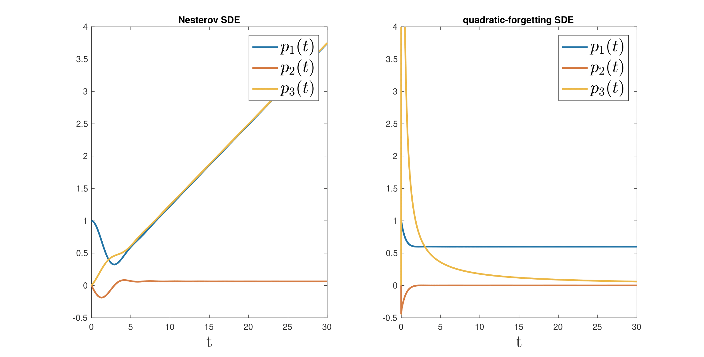
Figure 8: Numerical solution with MATLAB ode45 to Eq. (8) (on the left) and Eq. (9) (on the right). We choose $\lambda=\sigma=1$, but the results do not change qualitatively (only scale the axis) for $\sigma,\lambda_{i}\in{\mathbb{R}}_{+}$.

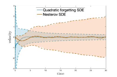
Figure 9: Simulation using Milstein scheme [Mil’shtejn, 1975] (stepsize $10^{-3}$, equivalent for this case to Euler-Maruyama) to verify covariance explosion of Nesterov’s SDE under a quadratic one dimensional cost $f(x)=x^{2}/2$. Plotted is the empirical mean and standard deviation of the velocity variable using 1000 runs. The dashed lines indicate the predictions from Eq. (8) and Eq. (9) (both solved numerically with MATLAB ode45 along with standard Nesterov’s ODE to get the mean). MG-SDE with quadratic forgetting has decreasing variance. Nesterov’s SDE amplifies linearly the negative gradient, and such amplification makes the velocity noisy, with exploding variance.

From the simulation results we conclude that, in the convex quadratic setting, the covariance of $V_{N}(t)$ explodes, while the one of $V_{{\mathfrak{m}}2}(t)$ does not: it converges. Indeed, as we show formally in App. D, for quadratic forgetting we get convergence to a ball around the solution. We validate these findings with a numerical simulation in Fig. 9.

Appendix D Proofs of convergence rates for the memory SDE

We start by refreshing the reader’s knowledge in stochastic calculus. Basic definitions (SDEs, stochastic integrals, etc) can be found in [Mao, 2007].

D.1 Stochastic calculus for the memory SDE

Consider the memory SDE

$$\begin{cases}dX(t)=V(t)dt\\ dV(t)=-\frac{\dot{\mathfrak{m}}(t)}{{\mathfrak{m}}(t)}V(t)dt-\frac{\dot{\mathfrak{m}}(t)}{{\mathfrak{m}}(t)}\nabla f(X(t))dt-\frac{\dot{\mathfrak{m}}(t)}{{\mathfrak{m}}(t)}\sigma(X(t),t)dB(t)\end{cases}.$$

We can rewrite this in vector notation ($0_{d\times d}$ is the $d\times d$ of all zeros)

$$\begin{pmatrix}dX(t)\\ dV(t)\end{pmatrix} =\begin{pmatrix}V(t)\\ -\frac{\dot{\mathfrak{m}}(t)}{{\mathfrak{m}}(t)}V(t)-\frac{\dot{\mathfrak{m}}(t)}{{\mathfrak{m}}(t)}\nabla f(X(t))\end{pmatrix}dt+\begin{pmatrix}0_{d\times d}&0_{d\times d}\\ 0_{d\times d}&-\frac{\dot{\mathfrak{m}}(t)}{{\mathfrak{m}}(t)}\sigma(X(t),t)\end{pmatrix}dB(t)$$

$$=b(X(t),V(t),t)dt+\xi(X(t),V(t),t)dB(t),$$ (10)

where $\{B(t)\}_{t\geq 0}$ is a d-dimensional Brownian Motion. We write this for simplicity as $b(t)dt+\xi(t)dt$.

Let $\mathcal{E}:{\mathbb{R}}^{d}\times{\mathbb{R}}^{d}\times{\mathbb{R}}\to{\mathbb{R}}$ be twice continuously differentiable jointly in the first two variables (indicated as $x$ and $v$) and continuously differentiable in the last (which we indicate as $t$). Then, by Itô’s lemma [Mao, 2007], the stochastic process $\{\mathcal{E}(X(t),V(t),t)\}_{t\geq 0}$ satisfies the following SDE:

$$d\mathcal{E}(X(t),V(t),t)=\partial_{t}\mathcal{E}(X(t),V(t),t))dt+\langle\partial_{(x,v)}\mathcal{E}(X(t),V(t),t),b(t)\rangle dt\\ +\frac{1}{2}\text{Tr}\left(\xi(t)\xi(t)^{T}\partial^{2}_{(x,v)}\mathcal{E}(X(t),V(t),t)\ \right)dt+\langle\partial_{(x,v)}\mathcal{E}(X(t),V(t),t),\xi(t)dB(t)\rangle.$$ (11)

where $\partial_{(x,v)}$ is the partial derivative with respect to $(x,v)$ and $\partial^{2}_{(x,v)}$ the matrix of second derivatives with respect to $(x,v)$. Notice that, in the deterministic case $\xi(t)=0$, the equation reduces to standard differentiation using the chain rule:

$$\frac{d\mathcal{E}(X(t),V(t),t)}{dt}=\partial_{t}\mathcal{E}(X(t),V(t)t))+\langle\partial_{(x,v)}\mathcal{E}(X(t),V(t),t),b(t)\rangle.$$

Following [Mao, 2007], we introduce the Itô diffusion differential operator $\mathscr{A}$ associated with Eq. (10) acting on a scalar function :

$$\mathscr{A}(\cdot)=\partial_{t}(\cdot)+\langle\partial_{(x,v)}(\cdot),b(t)\rangle+\frac{1}{2}\text{Tr}\left(\xi(t)\xi(t)^{T}\partial^{2}_{(x,v)}(\cdot)\right).$$ (12)

It is then clear that, thanks to Itô’s lemma,

$$d\mathcal{E}(X(t),V(t),t)=\mathscr{A}\mathcal{E}(X(t),V(t),t)dt+\langle\partial_{(x,v)}\mathcal{E}(X(t),V(t),t),\xi(t)dB(t)\rangle.$$

The Itô diffusion differential operator generalizes the concept of derivative: in fact, with slight abuse of notation

$$\frac{{\mathbb{E}}\left[d\mathcal{E}(X(t),V(t),t)\right]}{dt}=\mathscr{A}\mathcal{E}(X(t),V(t),t).$$

Moreover, by the definition of the solution to an SDE (see [Mao, 2007]), we know that at any time $t>0$,

$$\mathcal{E}(X(t),V(t),t)=\mathcal{E}(x_{0},v_{0},0)+\int_{0}^{t}\mathscr{A}\mathcal{E}(X(s),V(s),s)ds+\int_{0}^{t}\partial_{x}\mathcal{E}(X(s),V(s),s)^{T}\sigma(s)dB(s).$$

Taking the expectation the stochastic integral vanishes and we have

$${\mathbb{E}}[\mathcal{E}(X(t),V(t),t)]-\mathcal{E}(x_{0},0)={\mathbb{E}}\left[\int_{0}^{t}\mathscr{A}\mathcal{E}(X(s),V(s),s)ds\right].$$ (13)

This result is known as Dynkin’s formula and generalizes the fundamental theorem of calculus to the stochastic setting.

D.2 Convergence rates for polynomial forgetting

We recall our assumptions below.

(H0c)     $f\in{\mathcal{C}}^{3}_{b}({\mathbb{R}}^{d},{\mathbb{R}}),\ \sigma_{*}^{2}:=\sup_{x}\|\sigma(x)\sigma(x)^{T}\|_{s}<\infty$.

(H1’)    $f:{\mathbb{R}}^{d}\to{\mathbb{R}}$ is $L$-smooth and there exist $x^{*}\in{\mathbb{R}}^{d}$ s.t. for all $x\in{\mathbb{R}}^{d}$, $\langle\nabla f(x),x-x^{*}\rangle\geq\tau(f(x)-f(x^{*}))$.

The last condition is known as weak-quasi-convexity, and generalizes convexity (convex functions are wqc with constant 1  [Hardt et al., 2018]). The next fundamental lemma can also be found in [Krichene and Bartlett, 2017]. Consider two symmetric $d-$dimensional square matrices $P$ and $Q$. We have

$$\text{Tr}(PQ)\leq d\cdot\|P\|_{s}\cdot\|Q\|_{s},$$

where $\|\cdot\|_{s}$ denotes the spectral norm.

Proof.

Let $P_{j}$ and $Q_{j}$ be the j-th row(column) of $P$ and $Q$, respectively.

$$\text{Tr}(PQ) =\sum_{j=1}^{d}P_{j}^{T}Q_{j}\leq\sum_{j=1}^{d}\|P_{j}\|\cdot\|Q_{j}\|\leq\sum_{j=1}^{d}\|P\|_{s}\cdot\|Q\|_{s}=d\cdot\|P\|_{s}\cdot\|Q\|_{s},$$

where we first used the Cauchy-Schwarz inequality, and then the following inequality:

$$\|A\|_{s}=\sup_{\|z\|\leq 1}\|Az\|\geq\|Ae_{j}\|=\|A_{j}\|,$$

where $e_{j}$ is the j-th vector of the canonical basis of $\mathbb{R}^{d}$. ∎

We start with a general result about convergence of the memory SDE (see Sec. 3 of the main paper) for arbitrary memory ${\mathfrak{m}}(\cdot)$ in the stochastic setting. We will then specialize this result to polynomial forgetting.

[Continuous-time Convex Master Inequality] Assume (H0) and (H1’) hold. Let $\{X(t),V(t)\}_{t\geq 0}$ be a solution to MG-SDE with memory ${\mathfrak{m}}(\cdot)$, define $\lambda(t):=-{\mathfrak{m}}(t)\int\frac{1}{{\mathfrak{m}}(t)}dt$ (where $\int$ denotes the antiderivative) and $r(t):=\frac{\dot{\mathfrak{m}}(t)}{{\mathfrak{m}}(t)}\lambda(t)^{2}$. If ${\mathfrak{m}}(\cdot)$ is such that $\dot{r}(t)\leq\tau\lambda(t)\frac{\dot{\mathfrak{m}}(t)}{{\mathfrak{m}}(t)}$, then for any $t>0$

$${\mathbb{E}}[f(X(t))-f(x^{*})]\leq\frac{r(0)(f(x_{0})-f(x^{*}))+\frac{1}{2}\|x_{0}-x^{*}\|^{2}}{r(t)}+\ \frac{d\sigma^{2}_{*}}{2}\ \frac{\int_{0}^{t}\lambda(s)^{2}\left(\frac{\dot{\mathfrak{m}}}{{\mathfrak{m}}}(s)\right)^{2}ds}{r(t)}.$$

Proof.

Consider the following Lyapunov function, inspired from [Su et al., 2016]:

$$\mathcal{E}(x,v,t)=r(t)(f(x)-f(x^{*}))+\frac{1}{2}\|x-x^{*}+\lambda(t)v\|^{2},$$

where $r:{\mathbb{R}}\to{\mathbb{R}}$ and $\lambda:{\mathbb{R}}\to{\mathbb{R}}$ are two differentiable functions which we will fix during the proof. First, we find a bound on the infinitesimal diffusion generator of the stochastic process $\{\mathcal{E}(X(t),V(t),t)\}_{t\geq 0}$. Ideally, we want this bound to be independent of the dynamics (i.e the solution $\{(X(t),V(t))\}_{t\geq 0}$) of the problem, so that we can integrate it and get a rate.

By Itô’s lemma, we know that

$$\mathscr{A}\mathcal{E}(X(t),V(t),t) =\partial_{t}\mathcal{E}(X(t),V(t),t))dt+\langle\partial_{(x,v)}\mathcal{E}(X(t),V(t),t),b(t)\rangle dt$$

$$\ \ \ \ +\frac{1}{2}\text{Tr}\left(\xi(t)\xi(t)^{T}\partial^{2}_{x}\mathcal{E}(X(t),V(t),t)\ \right)dt.$$

Hence, plugging in the SDE definition and the definition of $\mathcal{E}$,

$$\mathscr{A}\mathcal{E}(X(t),V(t),t) =\partial_{t}\mathcal{E}(X(t),V(t),t))dt$$

$$\ \ \ \ +\langle\partial_{x}\mathcal{E}(X(t),V(t),t),V\rangle dt$$

$$\ \ \ \ +\left\langle\partial_{v}\mathcal{E}(X(t),V(t),t),-\frac{\dot{\mathfrak{m}}(t)}{{\mathfrak{m}}(t)}V(t)-\frac{\dot{\mathfrak{m}}(t)}{{\mathfrak{m}}(t)}\nabla f(X(t))\right\rangle dt$$

$$\ \ \ \ +\frac{1}{2}\text{Tr}\left(\xi(t)\xi(t)^{T}\partial^{2}_{(x,v)}\mathcal{E}(X(t),V(t),t)\ \right)dt$$

$$=\dot{r}(t)(f(X(t))-f(x^{*}))dt+2\langle X-x^{*}+\lambda(t)V,\dot{\lambda}(t)V\rangle dt$$

$$\ \ \ \ +r(t)\langle\nabla f(X),V\rangle dt+\langle X-x^{*}+\lambda(t)V,V\rangle dt$$

$$\ \ \ \ +\lambda(t)\left\langle X-x^{*}+\lambda(t)V,-\frac{\dot{\mathfrak{m}}(t)}{{\mathfrak{m}}(t)}V(t)-\frac{\dot{\mathfrak{m}}(t)}{{\mathfrak{m}}(t)}\nabla f(X)\right\rangle dt$$

$$\ \ \ \ +\frac{1}{2}\text{Tr}\left(\xi(t)\xi(t)^{T}\partial^{2}_{(x,v)}\mathcal{E}(X(t),V(t),t)\ \right)dt.$$

Next, we group some terms together,

$$\mathscr{A}\mathcal{E}(X(t),V(t),t) =\dot{r}(t)(f(X)-f(x^{*}))dt-\lambda(t)\frac{\dot{\mathfrak{m}}(t)}{{\mathfrak{m}}(t)}\langle\nabla f(X),X-x^{*}\rangle dt$$

$$\ \ \ \ +\left(\dot{\lambda}(t)+1-\lambda(t)\frac{\dot{\mathfrak{m}}(t)}{{\mathfrak{m}}(t)}\right)\left\langle X-x^{*}+\lambda(t)V,V\right\rangle dt$$

$$\ \ \ \ +\left(r(t)-\lambda(t)^{2}\frac{\dot{\mathfrak{m}}(t)}{{\mathfrak{m}}(t)}\right)\left\langle\nabla f(X),V\right\rangle dt$$

$$\ \ \ \ +\frac{1}{2}\text{Tr}\left(\xi(t)\xi(t)^{T}\partial^{2}_{(x,v)}\mathcal{E}(X(t),V(t),t)\ \right)dt.$$

Using (H1’), we conclude

$$\mathscr{A}\mathcal{E}(X(t),V(t),t) \leq\ \ \ \left(\dot{r}(t)-\tau\lambda(t)\frac{\dot{\mathfrak{m}}(t)}{{\mathfrak{m}}(t)}\right)(f(X)-f(x^{*}))dt$$

$$\ \ \ \ +\left(\dot{\lambda}(t)+1-\lambda(t)\frac{\dot{\mathfrak{m}}(t)}{{\mathfrak{m}}(t)}\right)\left\langle X-x^{*}+\lambda(t)V,V\right\rangle dt$$

$$\ \ \ \ +\left(r(t)-\lambda(t)^{2}\frac{\dot{\mathfrak{m}}(t)}{{\mathfrak{m}}(t)}\right)\left\langle\nabla f(X),V\right\rangle dt$$

$$\ \ \ \ +\frac{1}{2}\text{Tr}\left(\xi(t)\xi(t)^{T}\partial^{2}_{(x,v)}\mathcal{E}(X(t),V(t),t)\ \right)dt.$$

Under the hypotheses of this lemma, since $\dot{\lambda}(t)=\frac{\dot{\mathfrak{m}}(t)}{{\mathfrak{m}}(t)}\lambda(t)-1$ if and only if $\lambda(t)=-{\mathfrak{m}}(t)\int\frac{1}{{\mathfrak{m}}(t)}dt$, we are left with

$$\mathscr{A}\mathcal{E}(X(t),V(t),t) \leq\frac{1}{2}\text{Tr}\left(\xi(t)\xi(t)^{T}\partial^{2}_{(x,v)}\mathcal{E}(X(t),V(t),t)\ \right)dt$$

$$=\frac{d}{2}\left(\frac{\dot{\mathfrak{m}}(t)}{{\mathfrak{m}}(t)}\right)^{2}\text{Tr}\left(\sigma(t)\sigma(t)^{T}\partial^{2}_{v}\mathcal{E}(X(t),V(t),t)\right)dt$$

$$\leq\frac{d}{2}\left(\frac{\dot{\mathfrak{m}}(t)}{{\mathfrak{m}}(t)}\right)^{2}\|\sigma(t)\sigma(t)^{T}\|_{s}\|\partial^{2}_{v}\mathcal{E}(X(t),V(t),t)\|_{s}dt$$

$$\leq\frac{d}{2}\sigma^{2}_{*}\lambda(t)^{2}\left(\frac{\dot{\mathfrak{m}}(t)}{{\mathfrak{m}}(t)}\right)^{2}dt,$$

where in the first inequality we used Lemma D.2 and the definition of $\sigma^{2}_{*}$ in (H0c). Finally, by Dynkin’s formula

$${\mathbb{E}}[\mathcal{E}(X(t),V(t),t)]-\mathcal{E}(x_{0},0)\leq\frac{d\sigma^{2}_{*}}{2}\int_{0}^{t}\lambda(s)^{2}\left(\frac{\dot{\mathfrak{m}}}{{\mathfrak{m}}}(s)\right)^{2}ds;$$

therefore

$$r(t){\mathbb{E}}[f(X(t))-f(x^{*})]+{\mathbb{E}}\left[\frac{1}{2}\|X(t)-x^{*}+\lambda(t)V\|^{2}\right]\\ \leq r(0)(f(x_{0})-f(x^{*}))+\frac{1}{2}\|x_{0}-x^{*}\|^{2}+\frac{d\sigma^{2}_{*}}{2}\int_{0}^{t}\lambda(s)^{2}\left(\frac{\dot{\mathfrak{m}}}{{\mathfrak{m}}}(s)\right)^{2}ds,$$ (14)

which implies

$$r(t){\mathbb{E}}[f(X)-f(x^{*})]\leq r(0)(f(x_{0})-f(x^{*}))+\frac{1}{2}\|x_{0}-x^{*}\|^{2}+\frac{d\sigma^{2}_{*}}{2}\int_{0}^{t}\lambda(s)^{2}\left(\frac{\dot{\mathfrak{m}}}{{\mathfrak{m}}}(s)\right)^{2}ds.$$

∎

Under the conditions of Lemma D.2, let ${\mathfrak{m}}(t)=t^{p}$, with $p\geq 1+\frac{1}{\tau}$. Then, for any $t>0$,

$${\mathbb{E}}[f(X(t))-f(x^{*})]\leq\underbrace{\frac{(p-1)^{2}\|x_{0}-x^{*}\|^{2}}{2pt}}_{\text{rate of convergence to suboptimal sol.}}+\ \underbrace{\frac{p\ d\ \sigma^{2}_{*}}{2}}_{\text{suboptimality}}.$$

Proof.

This is a simple application of Lemma D.2. Since $p\neq 1$, we have $\lambda(t)=-{\mathfrak{m}}(t)\int\frac{1}{{\mathfrak{m}}(t)}dt=-t^{p}\int\frac{1}{t^{p}}dt=-t^{p}\left(\frac{t^{1-p}}{1-p}-C\right)$. Let us choose $C=0$, then $\lambda(t)=\frac{t}{p-1}$ and $r(t)=\frac{\dot{\mathfrak{m}}(t)}{{\mathfrak{m}}(t)}\lambda(t)^{2}=\frac{p}{t}\frac{t^{2}}{(p-1)^{2}}=\frac{pt}{(p-1)^{2}}$. Thanks to the Lemma, we get a rate if $\dot{r}(t)\leq\tau\lambda(t)\frac{\dot{\mathfrak{m}}(t)}{{\mathfrak{m}}(t)}$; that is, $\frac{p}{(p-1)^{2}}\leq\tau\frac{t}{p-1}\frac{p}{t}$, which is true if and only if $p\geq 1+\frac{1}{\tau}$. Plugging in the functions $h,{\mathfrak{m}}$ and $r$, we get the desired rate. ∎

Remark D.1 (Effect of starting integration after 0).

We start again from the rate in Lemma D.2, in the setting of Thm. D.2. We consider integration on an interval $[\epsilon,t]$ with $X_{\epsilon}(\epsilon)=x_{0}$ and $V_{\epsilon}(\epsilon)=0$:

$${\mathbb{E}}[f(X_{\epsilon}(t))-f(x^{*})]\leq\frac{\frac{p\epsilon}{(p-1)^{2}}(f(x_{0})-f(x^{*}))+\frac{1}{2}\|x_{0}-x^{*}\|^{2}}{r(t)}+\ \frac{pd\sigma^{2}_{*}}{2}\frac{t-\epsilon}{t}\ .$$

Trivially, as $\epsilon$ goes to $0$ and for any $t\geq 0$, we converge to the solution of Thm. D.2, which has to be intended as a limit case.

D.3 Convergence rates for exponential forgetting

We recall again our assumptions below.

(H0c)     $f\in{\mathcal{C}}^{3}_{b}({\mathbb{R}}^{d},{\mathbb{R}}),\ \sigma_{*}^{2}:=\sup_{x\in{\mathbb{R}}^{d}}\|\sigma(x)\sigma(x)^{T}\|_{s}<\infty$.

(H1)     $f:{\mathbb{R}}^{d}\to{\mathbb{R}}$ is $L$-smooth and convex.

(H2)     $f:{\mathbb{R}}^{d}\to{\mathbb{R}}$ is $\mu$-strongly convex.

(H1’)   $f:{\mathbb{R}}^{d}\to{\mathbb{R}}$ is $L$-smooth and there exists $x\in{\mathbb{R}}^{d}$ s.t. for all $x\in{\mathbb{R}}^{d}$, $\langle\nabla f(x),x-x^{*}\rangle\geq\tau(f(x)-f(x^{*})).$

(H2’)   $f:{\mathbb{R}}^{d}\to{\mathbb{R}}$ is such that, for all $x\in{\mathbb{R}}^{d}$ we have quadratic growth w.r.t $x^{*}\in{\mathbb{R}}^{d}$: $f(x)-f(x^{*})\geq\frac{\mu}{2}\|x-x^{*}\|^{2}$.

Remark D.2.

Convexity (i.e. (H1)) implies weak-quasi-convexity (H1’) with $\tau=1$  [Hardt et al., 2018]. Similarly, $\mu$- strong-convexity (i.e. (H2)) implies (H1’) with $\tau=1$ and (H2’) with the same $\mu$ [Karimi et al., 2016].

In this subsection, we are going to study the simplified stochastic exponential forgetting system

$$\begin{cases}dX(t)=V(t)dt\\ dV(t)=-\alpha V(t)dt-\alpha\left[\nabla f(X(t))dt+\sigma(X(t))dB(t)\right]\end{cases}.$$ (MG-SDE-exp)

We can rewrite this in vector notation

$$\begin{pmatrix}dX(t)\\ dV(t)\end{pmatrix} =\begin{pmatrix}V(t)\\ -\alpha V(t)-\alpha\nabla f(X(t))\end{pmatrix}dt+\begin{pmatrix}0_{d\times d}&0_{d\times d}\\ 0_{d\times d}&-\alpha\sigma(X(t))\end{pmatrix}dB(t)$$

$$=b(X(t),V(t),t)dt+\xi(X(t))dB(t),$$

which we write for simplicity as $b(t)dt+\xi(t)dB$. Existence and uniqueness of the solution to this SDE follows directly from [Mao, 2007].

D.3.1 Result under weak-quasi-convexity

Below is the main result for this subsection.

Assume (H0c) and (H1’) hold. Let $\{X(t),V(t)\}_{t\geq 0}$ be the stochastic process which solves MG-SDE-exp for $t\geq 0$, starting from $X(0)=x_{0}$ and $V(0)=0$. Then, for $t>0$ we have

$${\mathbb{E}}\left[f(X(\tilde{t}))-f(x^{*})\right]\leq\underbrace{\frac{\left(f(x_{0})-f(x^{*})\right)+\frac{\alpha}{2}\|x_{0}-x^{*}\|^{2}}{\alpha\tau t}}_{\text{rate of convergence to suboptimal sol.}}+\underbrace{\frac{d}{2\tau}\sigma^{2}_{*}}_{\text{suboptimality}},$$

where $\tilde{t}$ is sampled uniformly in $[0,t]$. Moreover, if (H1) holds (and therefore $\tau=1$), we can replace $X(\tilde{t})$ with the Cesàro average $\bar{X}(t)=\int_{0}^{t}X(s)ds$.

Remark D.3.

Notice that the suboptimality does not depend on the viscosity $\alpha$ and is exactly the same as for the SGD model [Orvieto and Lucchi, 2018]. This would not happen if we erase $\alpha$ in front of the gradient (i.e. the standard Heavy Ball model $\ddot{X}+\alpha\dot{X}+\nabla f(X)=0$ [Yang et al., 2018]).

Proof.

Consider $\mathcal{E}(x,t):=\alpha\left(f(x)-f(x^{*})\right)+\frac{1}{2}\|v+\alpha(x-x^{*})\|^{2}$. Using Eq. (11) we compute an upper bound on the infinitesimal diffusion generator of $\mathcal{E}$.

$$\mathscr{A}\mathcal{E}(X(t),V(t),t) =\cancel{\partial_{t}\mathcal{E}(X(t),V(t),t))dt}+\langle\partial_{(x,v)}\mathcal{E}(X(t),V(t),t),b(t)\rangle dt$$

$$\ \ \ \ +\frac{1}{2}\text{Tr}\left(\xi(t)\xi(t)^{T}\partial^{2}_{(x,v)}\mathcal{E}(X(t),V(t),t)\ \right)dt$$

$$=\langle\partial_{x}\mathcal{E}(X(t),V(t),t),V\rangle dt$$

$$\ \ \ \ +\left\langle\partial_{v}\mathcal{E}(X(t),V(t),t),-\alpha V(t)-\alpha\nabla f(X(t))\right\rangle dt$$

$$\ \ \ \ +\frac{1}{2}\text{Tr}\left(\xi(t)\xi(t)^{T}\partial^{2}_{(x,v)}\mathcal{E}(X(t),V(t),t)\ \right)dt$$

$$=\langle\alpha\nabla f(X(t))+\alpha(V(t)+\alpha(X(t)-x^{*})),V(t)\rangle dt$$

$$\ \ \ \ +\left\langle V(t)+\alpha(X(t)-x^{*}),-\alpha V(t)-\alpha\nabla f(X(t))\right\rangle dt$$

$$\ \ \ \ +\frac{1}{2}\text{Tr}\left(\alpha^{2}\sigma(t)\sigma(t)^{T}\partial^{2}_{(v,v)}\mathcal{E}(X(t),V(t),t)\ \right)dt$$

$$=\alpha\langle\nabla f(X(t)),V(t)\rangle dt+\alpha^{2}\langle X(t)-x^{*},V(t)\rangle+\alpha\|V(t)\|^{2}$$

$$\ \ \ \ -\alpha\|V(t)\|^{2}-\alpha\langle\nabla f(X(t)),V(t)\rangle-\alpha^{2}\langle V(t),X(t)-x^{*}\rangle-\alpha^{2}\langle\nabla f(X(t)),X(t)-x^{*}\rangle$$

$$\ \ \ \ +\frac{d}{2}\alpha^{2}\sigma^{2}_{*}$$

$$=-\alpha^{2}\langle\nabla f(X(t)),X(t)-x^{*}\rangle+\frac{d}{2}\alpha^{2}\sigma^{2}_{*}$$

$$\leq-\alpha^{2}\tau(f(X(t))-f(x^{*}))+\frac{d}{2}\alpha^{2}\sigma^{2}_{*}.$$

where in the first inequality we used Lemma D.2 and the definition of $\sigma^{2}_{*}$ in (H0c) and in the last we used (H1’). Finally, by Eq. (13)

$${\mathbb{E}}\left[\mathcal{E}(X(t),t)\right]-\mathcal{E}(x_{0},0)\leq-\alpha^{2}\tau\int_{0}^{t}{\mathbb{E}}[f(X(s))-f(x^{*})]ds+\frac{d}{2}\alpha^{2}\sigma^{2}_{*}t.$$

Since ${\mathbb{E}}\left[\mathcal{E}(X(t),t)\right]\geq 0$, we have

$$\alpha^{2}\tau\int_{0}^{t}{\mathbb{E}}[f(X(s))-f(x^{*})]ds\leq\mathcal{E}(x_{0},0)+\frac{d}{2}\alpha^{2}\sigma^{2}_{*}t;$$

Therefore

$${\mathbb{E}}\left[\int_{0}^{t}\frac{1}{t}f(X(s))-f(x^{*})ds\right]\leq\frac{\alpha\left(f(x_{0})-f(x^{*})\right)+\frac{\alpha^{2}}{2}\|x_{0}-x^{*}\|^{2}}{\alpha^{2}\tau t}+\frac{d}{2\tau}\sigma^{2}_{*}$$

Now, if $f(\cdot)$ is convex, we can use Jensen’s inequality and get the result directly. Otherwise, if $f(\cdot)$ is under (H1’), we can view the integral as the expectation of $f(X(\tilde{t}))-f(x^{*})$, where $\tilde{t}$ is sampled uniformly over $[0,t]$. ∎

D.3.2 Result under weak-quasi-convexity and quadratic growth

In the next proposition, we are going the consider a slightly generalized SDE

$$\begin{cases}dX(t)=V(t)dt\\ dV(t)=-\alpha V(t)dt-\nabla\tilde{f}(X(t))dt+\tilde{\sigma}(X(t))dB(t)\end{cases},$$ (MG-SDE-exp-G)

where $\tilde{f}(x)=Cf(x)$ and $\tilde{\sigma}(x)=C\sigma(x)$. We introduce this generalization to provide rates also for the stochastic counterpart of the standard Heavy-ball model $\ddot{X}+\alpha\dot{X}+\nabla f(X)=0$ generalizing [Shi et al., 2018] to any viscosity $\alpha$.

Further notation.

Under assumptions (H0c), (H1’), (H2’), we define the constants $\tilde{\sigma}_{*}^{2}$ and $\tilde{\mu}$ to match our assumptions: we have $\tilde{\sigma}_{*}^{2}:=\sup_{x\in{\mathbb{R}}^{d}}\|\tilde{\sigma}(x)\tilde{\sigma}(x)^{T}\|_{s}=C^{2}\sigma_{*}^{2}$, and $\tilde{f}(x)-\tilde{f}(x^{*})\geq\frac{\tilde{\mu}}{2}\|x-x^{*}\|^{2}:=\frac{C\mu}{2}\|x-x^{*}\|^{2}$.

Notice that MG-SDE-exp-G is exacly MG-SDE-exp for $\tilde{f}(\cdot)=\alpha f(\cdot)$ and $\tilde{\sigma}(\cdot)=\alpha\sigma(\cdot)$. However, it also contains the SDE of standard Heavy Ball in the case $\tilde{f}(\cdot)=f(\cdot)$ and $\tilde{\sigma}(\cdot)=\sigma(\cdot)$.

Assume (H0c), (H1’), (H2’) hold. Let $\{X(t),V(t)\}_{t\geq 0}$ be the stochastic process which solves MG-SDE-exp-G for $t\geq 0$ starting from $X(0)=x_{0}$ and $V(0)=0$. Then, for $t\geq 0$ we have

$${\mathbb{E}}[\tilde{f}(X(t))-\tilde{f}(x^{*})]\leq e^{-\gamma t}\left(\tilde{f}(x_{0})-\tilde{f}(x^{*})+\frac{(\alpha-\gamma)^{2}}{2}\|(x_{0}-x^{*})\|^{2}\right)+\frac{d}{2\gamma}\tilde{\sigma}_{*}^{2},$$ (15)

where

$$\begin{cases}\gamma=\frac{\tau}{\tau+2}\alpha&\text{for }\alpha\leq\alpha_{max}\\ \gamma=\frac{1}{2}\left(\alpha-\sqrt{\alpha^{2}-2\tilde{\mu}\tau}\right)&\text{for }\alpha\geq\alpha_{max}\\ \end{cases}$$

and $\alpha_{max}$ is the optimal viscosity parameter

$$\alpha_{max}=\frac{\tau+2}{2}\sqrt{\tilde{\mu}}.$$

We first need a lemma, of which we leave the proof to the reader.

Let $\tau,\beta,\tilde{\mu}$ be positive real numbers then

$$\frac{\tau\beta}{1+\frac{\beta^{2}}{\tilde{\mu}}}\geq\begin{cases}\frac{\tau}{2}\beta&\text{if }\beta\leq\sqrt{\tilde{\mu}}\\ \frac{\tau\tilde{\mu}}{2\beta}&\text{if }\beta\geq\sqrt{\tilde{\mu}}\end{cases}.$$

We illustrate this result graphically in Fig. 10 and proceed with the proof of the rate.

Figure 10: Bounds from Lemma D.3.2 for $\tau=0.5$ and $\tilde{\mu}=10$. The bounds overlap at $\sqrt{10}\simeq 3.13$.

Proof.

(of Prop. D.3.2) Define the following parametric energy

$$\mathcal{E}_{\gamma,\beta}(X(t),t):=e^{\gamma t}\left(\tilde{f}(X(t))-\tilde{f}(x^{*})+\frac{1}{2}\|V(t)+\beta(X(t)-x^{*})\|^{2}\right),$$

where $\beta$ and $\gamma$ are positive real numbers. The infinitesimal diffusion generator of $\mathcal{E}_{\gamma,\beta}(X(t),t)$ is

$$\mathscr{A}\mathcal{E}(X(t),V(t),t) =\underbrace{\partial_{t}\mathcal{E}(X(t),V(t),t)dt}_{\leavevmode\hbox to11.75pt{\vbox to11.75pt{\text{[drawing]}}}}+\underbrace{\langle\partial_{x}\mathcal{E}(X(t),V(t),t),V\rangle dt}_{\leavevmode\hbox to11.75pt{\vbox to11.75pt{\text{[drawing]}}}}$$

$$\ \ \ \ +\underbrace{\left\langle\partial_{v}\mathcal{E}(X(t),V(t),t),-\alpha V(t)-\alpha\nabla\tilde{f}(X(t))\right\rangle dt}_{\leavevmode\hbox to11.75pt{\vbox to11.75pt{\text{[drawing]}}}}$$

$$\ \ \ \ +\underbrace{\frac{1}{2}\text{Tr}\left(\xi(t)\xi(t)^{T}\partial^{2}_{(x,v)}\mathcal{E}(X(t),V(t),t)\ \right)dt}_{\leavevmode\hbox to11.75pt{\vbox to11.75pt{\text{[drawing]}}}}.$$

Using the definition of $\tilde{\sigma}_{*}^{2}$ and Lemma D.2, we can upper bound the generator with

$$\mathscr{A}\mathcal{E}(X(t),V(t),t) \leq\underbrace{\gamma e^{\gamma t}\left[\tilde{f}(X(t))-\tilde{f}(x^{*})+\frac{1}{2}\|V(t)+\beta(X(t)-x^{*})\|^{2}\right]dt}_{\leavevmode\hbox to11.75pt{\vbox to11.75pt{\text{[drawing]}}}}$$

$$\ \ \ +\underbrace{e^{\gamma t}\langle\nabla\tilde{f}+\beta V+\beta^{2}(X-x^{*}),V\rangle dt}_{\leavevmode\hbox to11.75pt{\vbox to11.75pt{\text{[drawing]}}}}\ \ \ +\underbrace{e^{\gamma t}\langle V+\beta(X-x^{*}),-\alpha V-\nabla\tilde{f}\rangle dt}_{\leavevmode\hbox to11.75pt{\vbox to11.75pt{\text{[drawing]}}}}+\underbrace{\frac{d}{2}e^{\gamma t}\tilde{\sigma}_{*}^{2}dt}_{\leavevmode\hbox to11.75pt{\vbox to11.75pt{\text{[drawing]}}}}.$$

Next, we multiply both sides by $\frac{e^{-\gamma t}}{dt}$ and proceeding with the calculations we get

$$\begin{split}\frac{e^{-\gamma t}\mathscr{A}\mathcal{E}}{dt}&=\gamma\tilde{f}(X(t))-\tilde{f}(x^{*})+\frac{\gamma}{2}\|V(t)+\beta(X(t)-x^{*})\|^{2}\\ &\ \ \ +\frac{d}{2}\tilde{\sigma}_{*}^{2}+\langle\nabla\tilde{f}+\beta V+\beta^{2}(X-x^{*}),V\rangle\\ &\ \ \ +\langle V+\beta(X-x^{*}),-\alpha V-\nabla\tilde{f}\rangle\\ &=\gamma\tilde{f}(X(t))-\tilde{f}(x^{*})+\frac{\gamma}{2}\|V\|^{2}+\frac{\beta^{2}\gamma}{2}\|X-x^{*}\|^{2}+\beta\gamma\langle V,X-x^{*}\rangle\\ &\ \ \ +\frac{d}{2}\tilde{\sigma}_{*}^{2}+\langle\nabla\tilde{f},V\rangle+\beta\|V\|^{2}+\beta^{2}\langle V,X-x^{*}\rangle\\ &\ \ \ -\alpha\|V\|^{2}-\langle\nabla\tilde{f},V\rangle-\alpha\beta\langle V,X-x^{*}\rangle-\beta\langle\nabla\tilde{f},X-x^{*}\rangle.\\ &\leq\left(\gamma+\frac{\beta^{2}\gamma}{\tilde{\mu}}-\beta\tau\right)\tilde{f}(X(t))-\tilde{f}(x^{*})+\frac{d}{2}\tilde{\sigma}_{*}^{2}\\ &\ \ \ +\left(\frac{\gamma}{2}+\beta-\alpha\right)\|V\|^{2}+(\beta\gamma+\beta^{2}-\alpha\beta)\langle V,X-x^{*}\rangle,\end{split}$$

where in the inequality we used (H1’) and (H2’). Next, since we a priori don’t have a way to bound the term $\langle V,X-x^{*}\rangle$ in general, we require

$$\gamma\beta+\beta^{2}-\alpha\beta=0,$$

which holds if and only if $\gamma+\beta=\alpha$. This also implies the coefficient multiplying $\|V\|^{2}$, that is $\left(\frac{\gamma}{2}+\beta-\alpha\right)$, is negative (because $\gamma$ and $\beta$ are positive).

Assume for now that $\left(\gamma+\frac{\beta^{2}\gamma}{\tilde{\mu}}-\beta\tau\right)\leq 0$ (we will deal with this at the end of this proof), we then get $\mathscr{A}\mathcal{E}\leq\frac{d}{2}\tilde{\sigma}_{*}^{2}e^{\gamma t}.$

Next, using Eq. (13),

$${\mathbb{E}}\left[\mathcal{E}_{\gamma,\beta}(X(t),t)\right]-\mathcal{E}_{\gamma,\beta}(x_{0},0)\leq\int_{0}^{t}\frac{d}{2}\tilde{\sigma}_{*}^{2}e^{\gamma s}ds.$$

Using the definition of $\mathcal{E}_{\gamma,\beta}$, we get

$$e^{\gamma t}{\mathbb{E}}\left[\tilde{f}(X(t))-\tilde{f}(x^{*})+\frac{1}{2}\|V(t)+\beta(X(t)-x^{*})\|^{2}\right]\\ \leq\tilde{f}(x_{0})-\tilde{f}(x^{*})+\frac{\beta^{2}}{2}\|(x_{0}-x^{*})\|^{2}+\int_{0}^{t}\frac{d}{2}\tilde{\sigma}_{*}^{2}e^{\gamma s}ds.$$

Hence, discarding the positive term $\frac{1}{2}\|V(t)+\beta(X(t)-x^{*})\|^{2}$ and multiplying both sides by $e^{-\gamma t}$ and solving the integral

$${\mathbb{E}}[\tilde{f}(X(t))-\tilde{f}(x^{*})] \leq e^{-\gamma t}\left(\tilde{f}(x_{0})-\tilde{f}(x^{*})\frac{\beta^{2}}{2}\|(x_{0}-x^{*})\|^{2}\right)+\frac{d}{2}\tilde{\sigma}_{*}^{2}\int_{0}^{t}e^{-\gamma(t-s)}ds$$

$$\leq e^{-\gamma t}\left(\tilde{f}(x_{0})-\tilde{f}(x^{*})\frac{\beta^{2}}{2}\|(x_{0}-x^{*})\|^{2}\right)+\frac{d}{2}\tilde{\sigma}_{*}^{2}\frac{1-e^{-\gamma t}}{\gamma}$$

$$\leq e^{-\gamma t}\left(\tilde{f}(x_{0})-\tilde{f}(x^{*})\frac{\beta^{2}}{2}\|(x_{0}-x^{*})\|^{2}\right)+\frac{d}{2\gamma}\tilde{\sigma}_{*}^{2},$$

which is the statement of the theorem. Now, we just need to choose $\beta$ and $\gamma$ such that $\left(\gamma+\frac{\beta^{2}\gamma}{\tilde{\mu}}-\beta\tau\right)<0$ while $\gamma+\beta=\alpha$. Since we have an inequality, we expect that the choice of $\beta$ and $\gamma$ is not unique. However, since $\gamma$ directly influences the rate, we would like it to be as large as possible. This can be formulated with the following linear program with nonlinear constrains.

$$(\gamma^{*},\beta^{*})=\begin{cases}\max_{\gamma,\beta}\ \ \ \gamma\\ \text{s.t}\ \ \ \ \ \ \ \ \ \ \ \gamma=\alpha-\beta\\ \ \ \ \ \ \ \ \ \ \ \ \ \ \ \ \gamma\leq\frac{\tau\beta}{1+\frac{\beta^{2}}{\tilde{\mu}}}\\ \ \ \ \ \ \ \ \ \ \ \ \ \ \ \ \gamma,\beta>0\end{cases}.$$

Using Lemma D.3.2, we shrink the feasible region at the cost of having a suboptimal, yet simpler, solution

$$(\gamma^{*},\beta^{*})=\begin{cases}\max_{\gamma,\beta}\ \ \ \gamma\\ \text{s.t}\ \ \ \ \ \ \ \ \ \ \ \gamma=\alpha-\beta\ \ \ \ \ \ \ \ \ \ \ \ \ \ \ \ \ \ \ \ \ \ (\bigcirc)\\ \ \ \ \ \ \ \ \ \ \ \ \ \ \ \ \gamma\leq\min\left\{\frac{\tau}{2}\beta,\frac{\tau\tilde{\mu}}{2\beta}\right\}\ \ \ \ \ \ \ (\mathord{\scalerel*{\Box}{gX}})\\ \ \ \ \ \ \ \ \ \ \ \ \ \ \ \ \gamma,\beta>0\end{cases}.$$

Figure 11: Bounds provided in Lemma D.3.2. Shown is the feasible region for the $\gamma$ maximization problem along with the optimal and approximate solution.

For any fixed $\alpha>0$, the RHS of $(\mathord{\scalerel*{\Box}{gX}})$ is positive and the RHS of $(\bigcirc)$ is a line which starts in $(\alpha,0)$ and eventually exist the set $\{\gamma,\beta)\ :\ \gamma\geq 0\}$. Hence, the constrain $(\mathord{\scalerel*{\Box}{gX}})$ is binding. The reader can find an helpful representation in Fig. 11. Notice now that we only have one feasible point, hence

$$(\gamma^{*},\beta^{*})=\begin{cases}\gamma=\alpha-\beta\\ \gamma=\min\left\{\frac{\tau}{2}\beta,\frac{\tau\tilde{\mu}}{2\beta}\right\}\\ \gamma,\beta>0\end{cases}.$$

Next, we ask when $\frac{\tau}{2}\beta=\frac{\tau\tilde{\mu}}{2\beta}$. This clearly happens at $\beta=\sqrt{\tilde{\mu}}$. This is the maximum of the continuous curve $\min\left\{\frac{\tau}{2}\beta,\frac{\tau\tilde{\mu}}{2\beta}\right\}$ with respect to $\beta$. The maximum achievable rate is therefore $\frac{\tau}{2}\sqrt{\tilde{\mu}}$ and it is reached for $\frac{\tau}{2}\sqrt{\tilde{\mu}}=\alpha-\sqrt{\tilde{\mu}}\Rightarrow\alpha=\frac{\tau+2}{2}\sqrt{\tilde{\mu}}$. Moreover, since $\frac{\tau\tilde{\mu}}{2\beta}$ and $\frac{\tau}{2}\beta$ only touch in one point, it is clear that

$$\gamma^{*}=\begin{cases}\frac{\tau}{2}\beta&\alpha\leq\frac{\tau+2}{2}\sqrt{\tilde{\mu}}\\ \frac{\tau\tilde{\mu}}{2\beta}&\alpha\geq\frac{\tau+2}{2}\sqrt{\tilde{\mu}}\end{cases}.$$

In any of these two regions, one just has equate the corresponding equation with $\gamma^{*}=\alpha-\beta^{*}$, to get

$$\gamma^{*}=\begin{cases}\frac{\tau}{\tau+2}\alpha&\text{for }\alpha\leq\frac{\tau+2}{2}\sqrt{\tilde{\mu}}\\ \frac{1}{2}\left(\alpha-\sqrt{\alpha^{2}-2\tilde{\mu}\tau}\right)&\text{for }\alpha\geq\frac{\tau+2}{2}\sqrt{\tilde{\mu}}\\ \end{cases}.$$

∎

From this general proposition, we derive results form the memory ODE and for the standard Heavy-ball ODE.

Assume (H0c), (H1), (H2) hold. Let $\{X(t),V(t)\}_{t\geq 0}$ be the stochastic process which solves MG-SDE-exp for $t\geq 0$ starting from $X(0)=x_{0}$ and $V(0)=0$. Then, for $t\geq 0$ we have

$${\mathbb{E}}[f(X(t))-f(x^{*})]\leq e^{-\gamma t}\left((f(x_{0})-f(x^{*}))+\frac{(\alpha-\gamma)^{2}}{2\alpha}\|(x_{0}-x^{*})\|^{2}\right)+\frac{d\alpha}{2\gamma}\sigma_{*}^{2}.$$ (16)

where

$$\begin{cases}\gamma=\frac{1}{3}\alpha&\text{for }\alpha\leq\alpha_{max}\\ \gamma=\frac{1}{2}\left(\alpha-\sqrt{\alpha^{2}-2\alpha\mu}\right)&\text{for }\alpha\geq\alpha_{max}\\ \end{cases}$$

and $\alpha_{max}$ is the optimal viscosity parameter

$$\alpha_{max}=\frac{9}{4}\mu.$$

Proof.

Follows directly from Prop. D.3.2 plugging in $\tau=1$, $\tilde{f}(x)=\alpha f(x)$, $\tilde{\mu}=\alpha\mu$ and $\tilde{\sigma}_{*}^{2}=\alpha^{2}\sigma_{*}^{2}$. ∎

Assume (H0c), (H1), (H2) hold. Let $\{X(t),V(t)\}_{t\geq 0}$ be the stochastic process which solves HB-SDE for $t\geq 0$, starting from $X(0)=x_{0}$ and $V(0)=0$. Then, for $t\geq 0$ we have

$${\mathbb{E}}[f(X(t))-f(x^{*})]\leq e^{-\gamma t}\left(f(x_{0})-f(x^{*})+\frac{(\alpha-\gamma)^{2}}{2}\|(x_{0}-x^{*})\|^{2}\right)+\frac{d\alpha}{2\gamma}\sigma_{*}^{2}.$$ (17)

where

$$\begin{cases}\gamma=\frac{1}{3}\alpha&\text{for }\alpha\leq\alpha_{max}\\ \gamma=\frac{1}{2}\left(\alpha-\sqrt{\alpha^{2}-2\mu}\right)&\text{for }\alpha\geq\alpha_{max}\\ \end{cases}$$

and $\alpha_{max}$ is the optimal viscosity parameter

$$\alpha_{max}=\frac{3}{2}\sqrt{\mu}.$$

Proof.

Follows directly from Prop. D.3.2 plugging in $\tilde{f}(x)=f(x)$, $\tau=1$, $\tilde{\mu}=\mu$ and $\tilde{\sigma}_{*}^{2}=\sigma_{*}^{2}$. ∎

The optimal rates are exponential for both SDEs; however, for MG-SDE-exp the constant in such exponential is proportional to $\sqrt{\mu}$, while for HB-SDE it is proportional to $\mu$. Note that this difference might be big if $\mu\ll 1$, leading to a faster rate for HB-SDE. However, this difference only comes because of the discretization procedure and will not be present in the algorithmic counterparts. Indeed, it is possible to show (we leave this exercise to the reader) that the optimal discretization stepsize $h$ for the first SDE (see Sec. 4 in the main paper) is $1/\sqrt{\mu L}$, while for the second SDE it is $2/(\sqrt{L}+\sqrt{\mu})=\mathcal{O}(1/\sqrt{L})$. Therefore, since we have the correspondence $t=kh$, in both cases we actually end up with $e^{\gamma_{max}t}\approx(1-C\sqrt{\mu/L})^{k}$, which is the well known accelerated rate found by [Polyak, 1964]. This interesting difference and the link to numerical integration deserves to be explored in a follow-up work.

Appendix E Provably convergent discrete-time polynomial forgetting

The algorithm below (a generalization of Heavy Ball) builds a sequence of iterates $\{x_{k}\}_{k\in{\mathbb{N}}}$ as well as moments $\{m_{k}\}_{k\in{\mathbb{N}}}$ starting from $m_{0}=0$ and using the recursion

$$m_{k+1} =\beta_{k}(x_{k}-x_{k-1})-\delta_{k}\eta\nabla f_{i_{k}}(x_{k})$$ (18)

$$x_{k+1} =x_{k}+m_{k+1}$$ (19)

where $i_{k}\in\{1,\dots,n\}$ is the index of a random data point sampled at iteration $k$, $\beta_{k}$ is an iteration-dependent positive momentum parameter and $\delta_{k}$ is a positive iteration-dependent discount on the learning rate $\eta$. Trivially, for each $x\in{\mathbb{R}}^{d}$, $f_{i_{k}}(x)$ is a random variable with mean zero and finite covariance matrix, which we call $\Sigma(x)$.

We list below two important assumptions

(H0d)    $\varsigma_{*}^{2}:=\sup_{x\in{\mathbb{R}}^{d}}\|\Sigma(x)\|_{s}<\infty$.

(H1)    $f:{\mathbb{R}}^{d}\to{\mathbb{R}}$ is convex and $L$-smooth.

We start with a rather abstract result inspired from [Ghadimi et al., 2015], which we will then use for algorithm design.

[Discrete-time Master Inequality] Assume (H1) and (H0d) hold. Let $\{\lambda_{k}\}_{k\in\mathbb{N}}$ be any sequence such that $\lambda_{k}\leq k$ for all $k$ and define $r_{k}=\eta(\lambda_{k}+1)$. If $\beta_{k}=\frac{\lambda_{k}}{\lambda_{k+1}+1}$, $\delta_{k}=\frac{1}{\lambda_{k+1}+1}$ and $\eta\leq 1/L$. Then we have for all iterates $\{x_{k}\}_{k\in{\mathbb{N}}}$ given by Eq. (18) and (19) that

$${\mathbb{E}}[f(x_{k})-f(x^{*})]\leq\frac{\|x_{0}-x^{*}\|^{2}}{2r_{k}}+\frac{d\eta^{2}\varsigma_{*}^{2}}{2}\frac{k}{r_{k}}.$$

Proof.

Consider the Lyapunov function inspired by the continuous-time setting in Lemma 3.1.

$$\mathcal{E}_{k}=r_{k}(f(x_{k})-f(x^{*}))+\frac{1}{2}\|x_{k+1}-x^{*}+\lambda_{k}m_{k+1}\|^{2}$$ (20)

First, notice that

$$x_{k+1}-x^{*}+\lambda_{k+1}m_{k+1} \overset{\eqref{eq:discrete_time_x}}{=}x_{k}-x^{*}+(1+\lambda_{k+1})m_{k+1}$$ (21)

$$\overset{\eqref{eq:discrete_time_m}}{=}x_{k}-x^{*}+(1+\lambda_{k+1})(\beta_{k}m_{k}-\delta_{k}\eta\nabla f_{i_{k}}(x_{k}))$$

$$=x_{k}-x^{*}+\lambda_{k}m_{k}-\eta\nabla f_{i_{k}}(x_{k})),$$

where in the last line we chose $\lambda_{k}=(\lambda_{k+1}+1)\beta_{k}$ and $\delta_{k}=\frac{1}{\lambda_{k}+1}$.

Consider $\zeta_{k}:=\nabla f_{i_{k}}(x_{k})-\nabla f(x_{k})$, then

$${\mathbb{E}}\left[\|x_{k+1}-x^{*}+\lambda_{k+1}m_{k+1}\|^{2}\right]= {\mathbb{E}}\left[\|x_{k}-x^{*}+\lambda_{k}m_{k}-\eta\nabla f(x_{k}))+\eta\zeta_{k}\|^{2}\right]$$

$$= {\mathbb{E}}\left[\|x_{k}-x^{*}+\lambda_{k}m_{k}\|^{2}\right]+{\mathbb{E}}\left[\|\eta\nabla f(x_{k})+\eta\zeta_{k}\|^{2}\right]$$

$$-2\eta{\mathbb{E}}\left[\langle\nabla f(x_{k}),x_{k}-x^{*}+\lambda_{k}m_{k}\rangle\right]$$

$$= {\mathbb{E}}\left[\|x_{k}-x^{*}+\lambda_{k}m_{k}\|^{2}\right]+\eta^{2}{\mathbb{E}}\left[\|\nabla f(x_{k})\|^{2}\right]+\eta^{2}{\mathbb{E}}\left[\|\zeta_{k}\|^{2}\right]$$

$$-2\eta{\mathbb{E}}\left[\langle\nabla f(x_{k}),x_{k}-x^{*}\rangle\right]-2\eta\lambda_{k}{\mathbb{E}}\left[\langle f(x_{k}),m_{k}\rangle\right].$$

Since $f(\cdot)$ is convex and smooth, it follows from Thm. 2.1.5 in [Nesterov, 2018] that

$$\dfrac{1}{L}\|\nabla f(x_{k})\|^{2} \leq\langle x_{k}-x^{*},\nabla f(x_{k})\rangle,$$

$$f(x_{k})-f(x^{*})+\dfrac{1}{2L}\|\nabla f(x_{k})\|^{2} \leq\langle x_{k}-x^{*},\nabla f(x_{k})\rangle,$$

$$f(x_{k})-f(x_{k-1}) \leq\langle x_{k}-x_{k-1},\nabla f(x_{k}))\rangle$$

for all $x_{k}$. Next, notice that $\zeta_{k}$ is a random variable with mean $0$ and we denote its covariance by $\Sigma(x_{k})\geq 0$. Moreover,

$${\mathbb{E}}\left[\|\zeta_{k}\|^{2}\right]={\mathbb{E}}\left[\text{Tr}(\zeta_{k}\zeta_{k}^{T})\right]=\text{Tr}({\mathbb{E}}\left[\zeta_{k}\zeta_{k}^{T}\right])=\text{Tr}(\Sigma(x_{k}))\leq d\|\Sigma(x_{k})\|_{s}=d\varsigma_{*}^{2}.$$

Let us assume $k\geq 1$, then

$${\mathbb{E}}\left[\|x_{k+1}-x^{*}+\lambda_{k+1}m_{k+1}\|^{2}\right]= {\mathbb{E}}\left[\|x_{k}-x^{*}+\lambda_{k}m_{k}\|^{2}\right]+\eta^{2}{\mathbb{E}}\left[\|\nabla f(x_{k})\|^{2}\right]+d\eta^{2}\varsigma_{*}^{2}$$

$$-2\eta{\mathbb{E}}\left[\langle\nabla f(x_{k}),x_{k}-x^{*}\rangle\right]-2\eta\lambda_{k}{\mathbb{E}}\left[\langle\nabla f(x_{k}),x_{k}-x_{k-1}\rangle\right]$$

$$\leq {\mathbb{E}}\left[\|x_{k}-x^{*}+\lambda_{k}m_{k}\|^{2}\right]+\eta^{2}{\mathbb{E}}\left[\|\nabla f(x_{k})\|^{2}\right]+d\eta^{2}\varsigma_{*}^{2}$$

$$-2\eta{\mathbb{E}}\left[f(x_{k})-f(x^{*})+\dfrac{1}{2L}\|\nabla f(x_{k})\|^{2}\right]-2\eta\lambda_{k}{\mathbb{E}}\left[f(x_{k})-f(x_{k-1})\right]$$

$$\leq {\mathbb{E}}\left[\|x_{k}-x^{*}+\lambda_{k}m_{k}\|^{2}\right]+\eta\left(\eta-\dfrac{1}{L}\right){\mathbb{E}}\left[\|\nabla f(x_{k})\|^{2}\right]+d\eta^{2}\varsigma_{*}^{2}$$

$$-2\eta(1+\lambda_{k}){\mathbb{E}}\left[f(x_{k})-f(x^{*})\right]+2\eta\lambda_{k}{\mathbb{E}}\left[f(x_{k-1})-f(x^{*})\right].$$

Then, let $\eta\leq 1/L$, note that ${\mathbb{E}}\left[f(x_{k})-f(x^{*})\right]\geq 0,\forall k$ and assume $\lambda_{k}\leq\lambda_{k-1}+1$. As a result, we have

$${\mathbb{E}}\left[\eta(1+\lambda_{k})(f(x_{k})-f(x^{*}))+\frac{1}{2}\|x_{k+1}-x^{*}+\lambda_{k+1}m_{k+1}\|^{2}\right]\\ \leq{\mathbb{E}}\left[\eta(1+\lambda_{k-1})(f(x_{k-1})-f(x^{*}))+\frac{1}{2}\|x_{k}-x^{*}+\lambda_{k}m_{k}\|^{2}\right]+\frac{d\eta^{2}\varsigma_{*}^{2}}{2}.$$

Recalling the definition of our Lyapunov function in Eq. (20) and choosing $r_{k}:=1+\lambda_{k}$, the last inequality reads as ${\mathbb{E}}[\mathcal{E}_{k}-\mathcal{E}_{k-1}]\leq\frac{d\eta^{2}}{2}\varsigma_{*}^{2}$ for $k\geq 1$ and by a telescoping sum argument we obtain

$${\mathbb{E}}[\mathcal{E}_{k}-\mathcal{E}_{0}]\leq\frac{d\eta^{2}\varsigma_{*}^{2}}{2}(k-1).$$

That is,

$${\mathbb{E}}\left[\eta(1+\lambda_{k})(f(x_{k})-f(x^{*}))\right]\leq{\mathbb{E}}\left[\eta(1+\lambda_{k})(f(x_{k})-f(x^{*}))+\frac{1}{2}\|x_{k+1}-x^{*}+\lambda_{k+1}m_{k+1}\|^{2}\right]\\ \leq{\mathbb{E}}\left[\eta(1+\lambda_{0})(f(x_{k-1})-f(x^{*}))+\frac{1}{2}\|x_{1}-x^{*}+\lambda_{1}m_{1}\|^{2}\right]+\frac{d\eta^{2}\varsigma_{*}^{2}}{2}(k-1).$$

Following the same procedure as above, we get

$${\mathbb{E}}\left[\frac{1}{2}\|x_{1}-x^{*}+\lambda_{1}m_{1}\|^{2}\right]\leq{\mathbb{E}}\left[\frac{1}{2}\|x_{0}-x^{*}\|^{2}\right]+\frac{d\eta^{2}}{2}\varsigma_{0}^{2}-\eta{\mathbb{E}}\left[f(x_{0})-f(x^{*})\right],$$

which can also be written as

$$\eta{\mathbb{E}}\left[f(x_{0})-f(x^{*})\right]+{\mathbb{E}}\left[\|x_{1}-x^{*}+\lambda_{1}m_{1}\|^{2}\right]\leq\frac{1}{2}\|x_{0}-x^{*}\|^{2}+\frac{d\eta^{2}\varsigma_{*}^{2}}{2}.$$

The proof is concluded once we set $\lambda_{0}=0$ ∎

We now apply the lemma above to get an algorithm and a convergence rate. In particular, we want to implement polynomial memory of past gradients and still get the rate found in Thm. D.2.

Assume (H1) and (H0d) hold. Consider the following iterative method

$$x_{k+1}=x_{k}+\frac{k}{k+p}(x_{k}-x_{k-1})-\frac{p}{k+p}\eta\nabla f_{i_{k}}(x_{k})$$

with $p\geq 2$ and $\eta\leq\frac{p-1}{pL}$. We have

$${\mathbb{E}}[f(x_{k})-f(x^{*})]\leq\underbrace{\frac{(p-1)^{2}\|x_{0}-x^{*}\|^{2}}{2\eta p(k+p-1)}}_{\text{rate of convergence to suboptimal sol.}}+\underbrace{\frac{1}{2}d\eta\varsigma_{*}^{2}p}_{\text{suboptimality}}.$$

Moreover, the resulting update direction can be written as $x_{k+1}-x_{k}=-\eta\sum_{i=0}^{k}w(i,k)\nabla f(x_{i})$ with $\sum_{i=0}^{k}w(i,k)=1$ and $w(\cdot,k):\{0,\dots,k\}\to{\mathbb{R}}$ behaving like a $(p-1)$-th order polynomial, that is $w(i,k)\sim i^{p-1}$, for all $k$.

Proof.

In the context of Lemma E, pick the continuous-time inspired (see definition of $\lambda(t)$ in the proof of Prop. D.2) function $\lambda_{k}=\frac{k}{p-1}\leq k$. If $r_{k}=\eta(\lambda_{k}+1)=\eta\frac{k+p-1}{p-1}$, $\beta_{k}=\frac{\lambda_{k}}{\lambda_{k+1}+1}=\frac{k}{k+p}$, $\delta_{k}=\frac{1}{\lambda_{k+1}+1}=\frac{p-1}{k+p}$, the iterates defined by

$$x_{k+1}=x_{k}+\frac{k}{k+p}(x_{k}-x_{k-1})-\frac{p-1}{k+p}\eta\nabla f_{i_{k}}(x_{k})$$

are such that, under $\eta\leq 1/L$,

$${\mathbb{E}}[f(x_{k})-f(x^{*})]\leq\frac{\|x_{0}-x^{*}\|^{2}}{2r_{k}}+\frac{d\eta^{2}\varsigma_{*}^{2}}{2}\frac{k}{r_{k}}=\frac{(p-1)\|x_{0}-x^{*}\|^{2}}{2\eta(k+p-1)}+\frac{d\eta\varsigma_{*}^{2}(p-1)}{2}\frac{k}{(k+p-1)}.$$

The algorithm above is similar to Eq (E). Indeed, if we define $\tilde{\eta}=\frac{p-1}{p}\eta$, then, under $\tilde{\eta}\leq\frac{p-1}{pL}$, the iterates defined by Eq (E) are such that

$${\mathbb{E}}[f(x_{k})-f(x^{*})]\leq\frac{(p-1)^{2}\|x_{0}-x^{*}\|^{2}}{2\tilde{\eta}p(k+p-1)}+\frac{1}{2}d\tilde{\eta}\varsigma_{*}^{2}p\frac{k}{(k+p-1)}\leq\frac{(p-1)^{2}\|x_{0}-x^{*}\|^{2}}{2\tilde{\eta}p(k+p-1)}+\frac{1}{2}d\tilde{\eta}\varsigma_{*}^{2}p.$$

Let us rename $\tilde{\eta}$ to $\eta$; it’s easy to realize by induction that

$$x_{k+1}-x_{k}=-\eta\sum_{j=0}^{k-1}\left(\prod_{h=j+1}^{k}\frac{h}{h+p}\right)\frac{p}{j+p}\nabla f(x_{j})-\eta\frac{p}{k+p}\nabla f(x_{k})=-\eta\sum_{j=0}^{k}w(j,k)\nabla f(x_{j}),$$

therefore, using some simple formulas from number theory

$$\sum_{j=0}^{k}w(j,k) =\sum_{j=0}^{k-1}\left(\prod_{h=j+1}^{k}\frac{h}{h+p}\right)\frac{p}{j+p}+\frac{p}{k+p}$$

$$=\sum_{j=0}^{k-1}\frac{(j+1)(j+2)\cdots\cancel{(j+p)}}{(k+1)(k+2)\cdots(k+p)}\frac{p}{\cancel{(j+p)}}+\frac{p}{k+p}$$

$$=\frac{p}{(k+1)(k+2)\cdots(k+p)}\sum_{j=0}^{k}(j+1)(j+2)\cdots(j+p-1),$$

From the last formula, we see that indeed the weights behave like a $(p-1)$-order polynomial. To conclude, notice that

$$\sum_{j=0}^{k}(j+1)(j+2)\cdots(j+p-1)=\frac{(k+1)(k+2)\cdots(k+p)}{p}.$$

∎

Appendix F Numerical simulation of memory and momentum ODEs

We recall below some ODEs we introduced throughout the paper.

Forgetting	corresponding viscosity in HB-ODE	MG-ODE
Constant	$\ddot{X}+\frac{1}{t}\dot{X}+\nabla f(X)=0$	$\ddot{X}+\frac{1}{t}\dot{X}+\frac{1}{t}\nabla f(X)=0$
Linear	$\ddot{X}+\frac{2}{t}\dot{X}+\nabla f(X)=0$	$\ddot{X}+\frac{2}{t}\dot{X}+\frac{2}{t}\nabla f(X)=0$
Quadratic	$\ddot{X}+\frac{3}{t}\dot{X}+\nabla f(X)=0$	$\ddot{X}+\frac{3}{t}\dot{X}+\frac{3}{t}\nabla f(X)=0$
Cubic	$\ddot{X}+\frac{4}{t}\dot{X}+\nabla f(X)=0$	$\ddot{X}+\frac{4}{t}\dot{X}+\frac{4}{t}\nabla f(X)=0$
Exponential($\alpha$)	$\ddot{X}+\frac{\alpha e^{\alpha t}}{e^{\alpha t}-1}\dot{X}+\nabla f(X)=0$	$\ddot{X}+\frac{\alpha e^{\alpha t}}{e^{\alpha t}-1}\dot{X}+\frac{\alpha e^{\alpha t}}{e^{\alpha t}-1}\nabla f(X)=0$
	$\approxeq\ddot{X}+\alpha\dot{X}+\nabla f(X)=0$	$\approxeq\ddot{X}+\alpha\dot{X}+\alpha\nabla f(X)=0$

Our setting is identical to the one outlined in Fig. 1 from [Su et al., 2016]: we consider the quadratic objective $f(x_{1},x_{2})=2\times 10^{-2}x_{1}^{2}+5\times 10^{-3}x_{2}^{2}$ and the numerical solution to the ODEs above starting from $X_{0}=(1,1)$ and $\dot{X}(0)=(0,0)$. The solution is computed using the MATLAB ode45 function, with absolute tolerance $10^{-10}$ end relative tolerance $10^{-5}$. We start integration at $t_{0}=2.2204\times 10^{-16}$ (machine precision). For numerical stability, when using exponential momentum and memory, we pick $\alpha=10$ and use the approximation $\frac{\alpha e^{\alpha t}}{e^{\alpha t}-1}\approxeq\alpha$ for large values of $t$. In the right part of the subplots, the dashed lines indicate the slope of the rates $1/t$, $1/t^{2}$, $1/t^{3}$, etc. Some comments follow.

1. As noted by [Su et al., 2016] in Thm. 8 of their paper , such second order equations can exhibit fast sublinear rates for quadratic objectives once the constant $p$ in the coefficient $p/t$ is increased.
   

2. To realize the worst-case rate in the convex setting, the reader can look at the slope of on the right plot before the first inverse peak: for instance, we see in the HB-ODE with $3/t$ viscosity that the slope is aligned with $1/t^{2}$, while linear forgetting is aligned with $1/t$. This is predicted by the time-warping presented in App. C.3.
   

3. As predicted again by App. C.3, $1/t$ viscosity has the same path as constant forgetting and $3/t$ viscosity goes along the same path as linear forgetting.

Appendix G Experiments on real-world datasets

G.1 Experimental setting

Datasets and architecture

We run four different sets of experiments. First, we optimize a logistic regression model on the covtype dataset ($n=464^{\prime}809$) from the popular LIBSVM library. This model is strongly convex and has $d=432$ parameters.

Secondly, we train an autoencoder introduced by [Hinton and Salakhutdinov, 2006] on the MNIST hand-written digits dataset ($n=60^{\prime}000$). The encoder structure is $784-1000-500-250-30$ and the decoder is mirrored. Sigmoid activations are used in all but the central layer. The reconstructed images are fed pixelwise into a binary cross entropy loss. The network has a total of $2^{\prime}833^{\prime}000$ parameters.

Third, we optimize a simple feed-forward network on the Fashion-MNIST dataset ($n=60^{\prime}000$). The network structure is $784-128-10$ with tanh activations in the hidden layer, cross entropy loss and a total of $101^{\prime}770$ parameters.

Finally, we train a fairly small convnet on the CIFAR-10 dataset ($n=50^{\prime}000$) taken from the official PyTorch tutorials (see here https://pytorch.org/tutorials/beginner/blitz/cifar10_tutorial.html.). The total number of parameters in this network amounts to $62^{\prime}006$.

Note that all neural networks models have sufficient expressive power to reach full training accuracy or (in the autoencoder case) reconstruct images very accurately. The linear model on covtype, however, achieves at most $\approx 70\%$ accuracy (see Fig.s 14 and 16).

Algorithms.

We benchmark several types of memory: (i) linear forgetting (p=2), (ii) cubic forgetting (p=4), higher degree polynomial forgetting (p=100) as well as exponential (p=e) and instantaneous forgetting (p=inf). Note that the last two algorithms exactly resemble Adam without adaptive preconditioning and vanilla SGD respectively. Furthermore, we also benchmark the classical Polyak Heavy Ball method (HB) as a reference point.

Parameters.

We run HB with a fixed momentum parameter $\beta=0.9$ across all experiments. For both SGD and HB we grid search the stepsize $\eta\in\{1,0.1,0.05,0.01,0.005,0.001,0.0005,0.0001,0.00005,0.00001\}$ and pick the best stepsize for each problem instance (reported in the corresponding legends). Interestingly, the best stepsize for HB is almost always one tenth of the SGD stepsize. The only exception is the convex logistic regression on covtype, where $\alpha_{SGD}=1$ was also the best stepsize for HB. There, we report $\alpha_{HB2}=0.1$ just for the sake of consistency. All versions of MemSGD simply run with the same stepsize as SGD, i.e. we did not grid-search the stepsize for MemSGD.

In order to assess the impact of stochasticity on SGD methods with memory, we run all algorithms in a large and a small batch setting. The large batch setting simply takes all training data points available in each dataset. For the small batch setting we chose the batch sizes as small as possible while still being able to train the networks in reasonable time. In particular, we take a mini-batch size of 16 for covtype and mnist. Fashion-mnist and Cifar-10 are run with 32 and 128 samples per iterations respectively.

All of our experiments are run using the PyTorch library [Paszke et al., 2017].  
 

Covtype Logreg	MNIST Autoencoder	FashionMNIST MLP	CIFAR-10 CNN

Figure 12: Real world experiments: Log loss over iterations in mini- (top) and full batch (bottom) setting. Average and $95\%$ confidence interval of 10 runs with random initialization.

Covtype Logreg	MNIST Autoencoder	FashionMNIST MLP	CIFAR-10 CNN

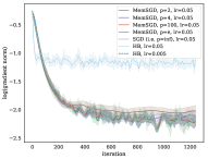
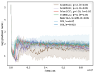
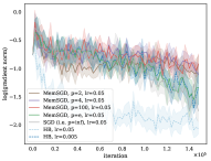
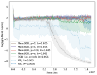
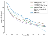
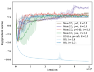
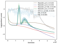
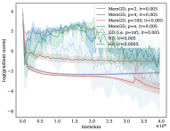
Figure 13: Real world experiments: Full gradient norm over iterations in mini- (top) and full batch (bottom) setting. Average and $95\%$ confidence interval of 10 runs with random initialization.

Covtype Logreg	FashionMNIST MLP	CIFAR-10 CNN

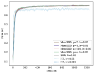
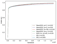
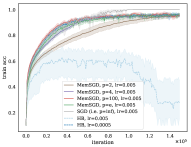
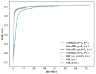
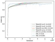
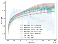
Figure 14: Real world experiments: Full training accuracy over iterations in mini- (top) and full batch (bottom) setting (undefined for autoencoder). Average and $95\%$ confidence interval of 10 runs with random initialization.

Covtype Logreg	MNIST Autoencoder	FashionMNIST MLP	CIFAR-10 CNN

Original
MemSGD (p=2)
MemSGD (p=4)
MemSGD (p=100)
MemSGD (p=e)
SGD (i.e. p=inf)
HB (lr=0.005)
HB (lr=0.05)

Figure 16: Original and reconstructed MNIST digits for different stochastic optimization methods after convergence. Compare Fig. 13 for corresponding loss.

References

- [Allen-Zhu, 2017] Allen-Zhu, Z. (2017). Katyusha: The first direct acceleration of stochastic gradient methods. In Proceedings of the 49th Annual ACM SIGACT Symposium on Theory of Computing, pages 1200–1205. ACM.
- [Arnol’d, 2013] Arnol’d, V. I. (2013). Mathematical methods of classical mechanics, volume 60. Springer Science & Business Media.
- [Betancourt et al., 2018] Betancourt, M., Jordan, M. I., and Wilson, A. C. (2018). On symplectic optimization. arXiv preprint arXiv:1802.03653.
- [Bottou et al., 2018] Bottou, L., Curtis, F. E., and Nocedal, J. (2018). Optimization methods for large-scale machine learning. SIAM Review, 60(2):223–311.
- [Cabot et al., 2009] Cabot, A., Engler, H., and Gadat, S. (2009). On the long time behavior of second order differential equations with asymptotically small dissipation. Transactions of the American Mathematical Society, 361:5983–6017.
- [Cauchy, 1847] Cauchy, A. (1847). Méthode générale pour la résolution des systemes d’équations simultanées. Comp. Rend. Sci. Paris, 25(1847):536–538.
- [Duchi et al., 2011] Duchi, J., Hazan, E., and Singer, Y. (2011). Adaptive subgradient methods for online learning and stochastic optimization. Journal of Machine Learning Research, 12(Jul):2121–2159.
- [Gadat and Panloup, 2014] Gadat, S. and Panloup, F. (2014). Long time behaviour and stationary regime of memory gradient diffusions. In Annales de l’IHP Probabilités et statistiques, volume 50, pages 564–601.
- [Ghadimi et al., 2015] Ghadimi, E., Feyzmahdavian, H. R., and Johansson, M. (2015). Global convergence of the heavy-ball method for convex optimization. In Control Conference (ECC), 2015 European, pages 310–315. IEEE.
- [Ghadimi and Lan, 2012] Ghadimi, S. and Lan, G. (2012). Optimal stochastic approximation algorithms for strongly convex stochastic composite optimization i: A generic algorithmic framework. SIAM Journal on Optimization, 22(4):1469–1492.
- [Goodfellow et al., 2016] Goodfellow, I., Bengio, Y., and Courville, A. (2016). Deep learning. MIT press.
- [Hairer et al., 2006] Hairer, E., Lubich, C., and Wanner, G. (2006). Geometric numerical integration: structure-preserving algorithms for ordinary differential equations, volume 31. Springer Science & Business Media.
- [Hardt et al., 2018] Hardt, M., Ma, T., and Recht, B. (2018). Gradient descent learns linear dynamical systems. The Journal of Machine Learning Research, 19(1):1025–1068.
- [Hinton and Salakhutdinov, 2006] Hinton, G. E. and Salakhutdinov, R. R. (2006). Reducing the dimensionality of data with neural networks. science, 313(5786):504–507.
- [Jain et al., 2018] Jain, P., Kakade, S. M., Kidambi, R., Netrapalli, P., and Sidford, A. (2018). Accelerating stochastic gradient descent for least squares regression. In Conference On Learning Theory, pages 545–604.
- [Karimi et al., 2016] Karimi, H., Nutini, J., and Schmidt, M. (2016). Linear convergence of gradient and proximal-gradient methods under the polyak-łojasiewicz condition. In Joint European Conference on Machine Learning and Knowledge Discovery in Databases, pages 795–811. Springer.
- [Khalil and Grizzle, 2002] Khalil, H. K. and Grizzle, J. (2002). Nonlinear systems, volume 3. Prentice hall Upper Saddle River, NJ.
- [Kidambi et al., 2018] Kidambi, R., Netrapalli, P., Jain, P., and Kakade, S. (2018). On the insufficiency of existing momentum schemes for stochastic optimization. In 2018 Information Theory and Applications Workshop (ITA), pages 1–9. IEEE.
- [Kingma and Ba, 2014] Kingma, D. P. and Ba, J. (2014). Adam: A method for stochastic optimization. arXiv preprint arXiv:1412.6980.
- [Krichene and Bartlett, 2017] Krichene, W. and Bartlett, P. L. (2017). Acceleration and averaging in stochastic descent dynamics. In Advances in Neural Information Processing Systems, pages 6796–6806.
- [Krichene et al., 2015] Krichene, W., Bayen, A., and Bartlett, P. L. (2015). Accelerated mirror descent in continuous and discrete time. In Advances in neural information processing systems, pages 2845–2853.
- [Lan, 2012] Lan, G. (2012). An optimal method for stochastic composite optimization. Mathematical Programming, 133(1-2):365–397.
- [Li et al., 2017] Li, Q., Tai, C., et al. (2017). Stochastic modified equations and adaptive stochastic gradient algorithms. In Proceedings of the 34th International Conference on Machine Learning-Volume 70, pages 2101–2110. JMLR. org.
- [Ma and Yarats, 2018] Ma, J. and Yarats, D. (2018). Quasi-hyperbolic momentum and adam for deep learning. arXiv preprint arXiv:1810.06801.
- [Mao, 2007] Mao, X. (2007). Stochastic differential equations and applications. Elsevier.
- [Mertikopoulos and Staudigl, 2018] Mertikopoulos, P. and Staudigl, M. (2018). On the convergence of gradient-like flows with noisy gradient input. SIAM Journal on Optimization, 28(1):163–197.
- [Mil’shtejn, 1975] Mil’shtejn, G. (1975). Approximate integration of stochastic differential equations. Theory of Probability & Its Applications, 19(3):557–562.
- [Nesterov, 2018] Nesterov, Y. (2018). Lectures on convex optimization. Springer.
- [Nesterov, 1983] Nesterov, Y. E. (1983). A method for solving the convex programming problem with convergence rate o (1/k^ 2). In Dokl. Akad. Nauk SSSR, volume 269, pages 543–547.
- [Øksendal, 2003] Øksendal, B. (2003). Stochastic differential equations. In Stochastic differential equations, pages 65–84. Springer.
- [Orvieto and Lucchi, 2018] Orvieto, A. and Lucchi, A. (2018). Continuous-time models for stochastic optimization algorithms. arXiv preprint arXiv:1810.02565.
- [Paszke et al., 2017] Paszke, A., Gross, S., Chintala, S., Chanan, G., Yang, E., DeVito, Z., Lin, Z., Desmaison, A., Antiga, L., and Lerer, A. (2017). Automatic differentiation in pytorch. In NIPS-W.
- [Polyak, 1964] Polyak, B. T. (1964). Some methods of speeding up the convergence of iteration methods. USSR Computational Mathematics and Mathematical Physics, 4(5):1–17.
- [Polyak, 1987] Polyak, B. T. (1987). Introduction to optimization. optimization software. Inc., Publications Division, New York, 1.
- [Reddi et al., 2018] Reddi, S., Kale, S., and Kumar, S. (2018). On the convergence of adam and beyond. In International Conference on Learning Representations.
- [Robbins and Monro, 1951] Robbins, H. and Monro, S. (1951). A stochastic approximation method. The annals of mathematical statistics, pages 400–407.
- [Shi et al., 2018] Shi, B., Du, S. S., Jordan, M. I., and Su, W. J. (2018). Understanding the acceleration phenomenon via high-resolution differential equations. arXiv preprint arXiv:1810.08907.
- [Shi et al., 2019] Shi, B., Du, S. S., Su, W. J., and Jordan, M. I. (2019). Acceleration via symplectic discretization of high-resolution differential equations. arXiv preprint arXiv:1902.03694.
- [Su et al., 2016] Su, W., Boyd, S., and Candes, E. J. (2016). A differential equation for modeling nesterov’s accelerated gradient method: Theory and insights. Journal of Machine Learning Research, 17:1–43.
- [Sutskever et al., 2013] Sutskever, I., Martens, J., Dahl, G., and Hinton, G. (2013). On the importance of initialization and momentum in deep learning. In Dasgupta, S. and McAllester, D., editors, Proceedings of the 30th International Conference on Machine Learning, volume 28 of Proceedings of Machine Learning Research, pages 1139–1147, Atlanta, Georgia, USA. PMLR.
- [Wibisono et al., 2016] Wibisono, A., Wilson, A. C., and Jordan, M. I. (2016). A variational perspective on accelerated methods in optimization. proceedings of the National Academy of Sciences, 113(47):E7351–E7358.
- [Wilson et al., 2016] Wilson, A. C., Recht, B., and Jordan, M. I. (2016). A lyapunov analysis of momentum methods in optimization. arXiv preprint arXiv:1611.02635.
- [Xu et al., 2018a] Xu, P., Wang, T., and Gu, Q. (2018a). Accelerated stochastic mirror descent: From continuous-time dynamics to discrete-time algorithms. In International Conference on Artificial Intelligence and Statistics, pages 1087–1096.
- [Xu et al., 2018b] Xu, P., Wang, T., and Gu, Q. (2018b). Continuous and discrete-time accelerated stochastic mirror descent for strongly convex functions. In International Conference on Machine Learning, pages 5488–5497.
- [Yang et al., 2018] Yang, L., Arora, R., Zhao, T., et al. (2018). The physical systems behind optimization algorithms. In Advances in Neural Information Processing Systems, pages 4377–4386.
- [Yang et al., 2016] Yang, T., Lin, Q., and Li, Z. (2016). Unified convergence analysis of stochastic momentum methods for convex and non-convex optimization. arXiv preprint arXiv:1604.03257.
- [Yuan et al., 2016] Yuan, K., Ying, B., and Sayed, A. H. (2016). On the influence of momentum acceleration on online learning. The Journal of Machine Learning Research, 17(1):6602–6667.
- [Zhang et al., 2018] Zhang, J., Mokhtari, A., Sra, S., and Jadbabaie, A. (2018). Direct runge-kutta discretization achieves acceleration. In Advances in Neural Information Processing Systems, pages 3904–3913.