Control-oriented model reduction for
minimizing transient energy growth in shear flows

Abstract

A linear non-modal mechanism for transient amplification of perturbation energy is known to trigger sub-critical transition to turbulence in many shear flows. Feedback control strategies for minimizing this transient energy growth can be formulated as convex optimization problems based on linear matrix inequalities. Unfortunately, solving the requisite linear matrix inequality problem can be computationally prohibitive within the context of high-dimensional fluid flows. In this work, we investigate the utility of control-oriented reduced-order models to facilitate the design of feedback flow control strategies that minimize the maximum transient energy growth. An output projection onto proper orthogonal decomposition modes is used to faithfully capture the system energy. Subsequently, a balanced truncation is performed to reduce the state dimension, while preserving the system’s input-output properties. The model reduction and control approaches are studied within the context of a linearized channel flow with blowing and suction actuation at the walls. Controller synthesis for this linearized channel flow system becomes tractable through the use of the proposed control-oriented reduced-order models. Further, the resulting controllers are found to reduce the maximum transient energy growth compared with more conventional linear quadratic optimal control strategies.

Keywords: Reduced-order model; transient energy growth; channel flow; feedback flow control; modal decomposition.

Nomenclature

$\Theta_{max}$  =	maximum transient energy growth
$\Phi_{r}$  =	matrix of $r$ dominant proper orthogonal decomposition modes
$(\alpha,\beta)$  =	streamwise and spanwise wave number pair
$A$  =	linear time invariant state matrix of plant
$\bar{A}$  =	reduced-order state matrix after balanced-truncation
$B$  =	linear time invariant input matrix of plant
$\bar{B}$  =	reduced-order input matrix after balanced-truncation
$E$  =	energy of the full-order plant
$\bar{E}$  =	reduced-order approximation of $E$
$K$  =	controller feedback gain
$Re$  =	Reynolds number
$T_{s}$  =	matrix of $s$ dominant balanced modes
$U_{cl}$  =	channel laminar base flow center-line velocity
$h$  =	channel half-height
$n$  =	dimension of the full-order plant
$q_{u},q_{l}$  =	wall-normal velocities at upper and lower wall respectively
$r,s$  =	number of proper orthogonal decomposition modes and balanced modes, respectively.
$\mathbf{u}$  =	input vector
$\mathbf{x}$  =	state vector
$\mathbf{z}$  =	proper orthogonal decomposition coefficients

1 Introduction

The transition of flows from a laminar to turbulent regime has been extensively studied, and remains a topic of continuing interest. It is well known that turbulent flows exhibit specific detrimental effects on systems, e.g., an increase in skin friction drag in wall-bounded shear flows [1]. It has been observed that transition to turbulence in many shear flows occurs at a Reynolds number ($Re$) much below the critical $Re$ predicted by linear (modal) stability analysis of a steady laminar base flow [2, 3]. This sub-critical transition is associated with non-modal amplification mechanisms that cause small disturbances to grow before undergoing an eventual modal decay, based on the linear analysis [4, 5, 6]. This transient energy growth (TEG) of disturbances can trigger non-linear instabilities and lead to bypass transition by driving the flow state beyond the region of attraction of the laminar equilibrium profile  [4, 7].

Numerous investigations have considered the possibility of reducing TEG and delaying transition by employing feedback control techniques. Excellent reviews of past works can be found in [8, 9, 10]. Linear quadratic optimal control has been a common approach for such applications. The full-information linear quadratic regulator (LQR) has been investigated in various capacities, and has been shown to increase transition thresholds within the channel flow system [11, 12, 13]. Observer-based output-feedback controllers have also been invoked with some success [11, 14, 15]. In [15], the authors successfully design a linear quadratic Gaussian (LQG) controller on a reduced-order Poiseuille flow system—combining the optimal LQR law with optimal state estimates from a Kalman filter. The study in [11] investigates LQG/$\mathcal{H}_{2}$ and $\mathcal{H}_{\infty}$ controllers, with particular emphasis on the use of appropriate transfer function norms to minimize the energy of flow perturbations in a channel flow system. The study in [14] further investigates LQG control of the channel flow system, giving careful attention to the design of the Kalman filter for optimal state estimation for use in observer-based feedback control. More recently, it has been shown that observer-based feedback strategies may exacerbate TEG in the controlled system, due to an adverse coupling between the fluid dynamics and the control system dynamics [16]. As a potential alternative, static output feedback formulations of the LQR problem have shown some promise in overcoming the limitations of LQG strategies under certain flow conditions within the channel flow system [17, 18]. Interestingly, although all of these investigations have shown the promise of feedback control for reducing TEG and delaying transition, it stands that linear quadratic optimal control techniques and related synthesis approaches do not necessarily minimize—nor even reduce—TEG. Indeed, in the case of LQR, the objective function to be minimized is the balance of integrated perturbation energy and input energy—not explicitly the TEG itself. Thus, the most commonly employed controller synthesis approaches aim to achieve an objective that does not necessarily address the TEG problem directly.

Given the central role of TEG and non-modal instabilities in the transition process, it seems that a more appropriate objective function for transition control would be to minimize the maximum transient energy growth (MTEG), as proposed in [19]. This objective has direct connections with notions of worst-case or optimal perturbations, which correspond to disturbances that result in the maximum TEG [20]. The objective also has connections with optimal forcing functions determined from input-output analysis [21], though these types of “persistent disturbances” will not be considered in the present work. The minimum-MTEG optimal control problem—which can be specified for either full-state or output feedback [19]—can be posed as a linear matrix inequality (LMI). The LMI constitutes a convex optimization problem that can be solved using standard methods, such as interior-point methods [22]. However, the specific LMI problem that arises for MTEG minimization is computationally intractable for high-order systems, such as fluid flows; the memory requirements associated with existing solution methods scale as system order to the sixth power [13].

Despite the computational challenge, control laws that minimize the MTEG can be desirable over linear quadratic optimal control techniques. MTEG-minimizing controllers have been found to outperform LQR controllers in reducing TEG within a channel flow configuration [13]. To achieve this, a modal truncation was performed to obtain a reduced-order model (ROM) that would make controller synthesis tractable for the linearized channel flow system [13]. In spite of the noteworthy performance reported in their study, it is well-established that modal truncation methods tend to yield ROMs that are poorly suited for controller synthesis [23, 24]. (A demonstration of this point is given in Appendix A.) Thus, it may be possible to synthesize MTEG-minimizing controllers with even better performance than those reported in [13] by exploiting an appropriately tailored control-oriented model reduction strategy.

Various ROM approaches have been studied in the literature (see [25, 26] for excellent reviews of such techniques within the context of fluid dynamics). However, developing ROMs that facilitate the design of MTEG-minimizing controllers requires a tailored approach. Control-oriented ROMs within this context must address a dual need: (i) approximate the perturbation energy to concisely and adequately describe the energy-based control objective; and (ii) reduce dimensionality to faithfully represent the input-output dynamics, as needed for computationally tractable controller synthesis. Identifying states that contribute substantially to both the perturbation energy and a system’s input-output properties (e.g., controllability and observability) is a non-trivial task [27]. A projection onto proper orthogonal decomposition (POD) modes is known to be optimal for capturing the energy of a given signal; however, projection-based model reduction based on POD modes often fails to capture a system’s input-output dynamics, making such models poor candidates for controller synthesis [28, 26]. In contrast, balanced truncation can be performed to obtain ROMs that retain a system’s input-output properties [29, 30]. The balanced truncation procedure can be shown to be equivalent to a Petrov-Galerkin ROM based on a projection onto a subspace spanned by a reduced set of balanced modes. For high-dimensional fluid flow systems, the balanced POD (BPOD) and related methods provide efficient tools for computing these balanced modes [27, 31, 30]. Alternative control-oriented model reduction techniques can also be devised to retain a system’s input-output properties, e.g., using ideas from robust control [24, 30].

The contribution of the present study is to investigate the utility of control-oriented model reduction for designing MTEG-minimizing controllers. The study focuses on full-information control of a linearized channel flow system, but the lessons learned can be generalized to other flows and control architectures as well. The ROMs in this work use POD and balanced truncation in conjunction. First, we perform an output-projection of the full-state onto a set of dominant POD modes. Subsequently, a balanced truncation is performed to reduce the state-dimension, while retaining the most controllable and observable modes that contribute to the input-output dynamics. As we will see, this dual approach results in control-oriented ROMs that can yield effective MTEG-minimizing controllers. The resulting models are able to represent the perturbation energy in terms of a small number of POD modes, thus providing a convenient approximation of the objective function. Further, state-dimension is reduced to a computationally tractable level, while retaining the most controllable and observable states that are critical for effective controller design.

The organization of the paper is as follows: Section 2 summarizes preliminaries on TEG and the relevant controller synthesis strategies, including the synthesis of LQR controllers and the LMI-based synthesis of MTEG-minimizing controllers. The control-oriented model reduction approach is then introduced in Section 2.1. Section 3 presents all of the results, which are based on the linearized channel flow system described in Section 3.1. ROMs are analyzed in an open-loop context in Section 3.2. Controller performance of ROM-based controller designs is evaluated in Section 3.3, which also includes a comparative analysis of the flow response to LQR and MTEG-minimizing control laws. Finally, Section 4 summarizes the findings and contributions of this study.

2 Reduced-order models and controller synthesis

Consider the linearized dynamics of flow perturbations $\mathbf{x}(t)$ about a steady laminar base-flow,

$$\dot{\mathbf{x}}(t)=A\mathbf{x}(t)+B\mathbf{u}(t)$$ (1)

where $\mathbf{x}$ is a vector of $n$ state variables, $\mathbf{u}$ is a vector of $p$ control inputs, and $t$ is time. Specific details on arriving at such a representation for a channel flow setup will be described in Section 3.1. The free-response of the system to an initial perturbation $\mathbf{x}(t_{o})=\mathbf{x}_{o}$ at time $t_{o}$ is given in terms of the matrix exponential $\mathbf{x}(t)=\mathrm{e}^{A(t-t_{o})}\mathbf{x}_{o}$. The perturbation energy for this system is defined as $E(t):=\mathbf{x}^{\mathsf{T}}(t)Q\mathbf{x}(t)$, where $Q=Q^{\mathsf{T}}>0$. In this study, we are primarily interested in the maximum transient energy growth (MTEG),

$$\Theta_{\text{max}}=\max_{t\geq t_{0}}\max_{E(t_{0})\neq 0}\frac{E(t)}{E(t_{0})},$$ (2)

which corresponds to the peak energy over all disturbances and all time. The flow perturbation $\mathbf{x}_{o}^{\text{opt}}$ that results in this MTEG is called the worst-case disturbance or the optimal perturbation [20].

Owing to the role of transient energy growth in sub-critical transition, our aim here will be to reduce the MTEG using full-information feedback control laws of the form $\mathbf{u}(t)=-K\mathbf{x}(t)$, where $K$ is a gain matrix determined by an appropriate synthesis strategy. In this study, two controller synthesis approaches will be considered: (i) linear quadratic regulation (LQR), and (ii) MTEG minimization via LMI-based synthesis. LQR is an optimal control technique that has been commonly employed in a variety of flow control applications, including transition control. LQR controllers are designed to minimize the integrated balance between perturbation energy and control effort; i.e.,

$$\min_{\mathbf{u}(t)}J=\int_{0}^{\infty}(\mathbf{x}^{T}Q\mathbf{x}+\mathbf{u}^{T}R\mathbf{u})dt$$ (3)

subject to the linear dynamic constraint in (1) and $R>0$. The feedback control law that minimizes this cost function is given by $\mathbf{u}=-K\mathbf{x}$, where the control gain $K=R^{-1}B^{T}P$ and $P=P^{\mathsf{T}}>0$ is determined from the algebraic Riccati equation,

$$A^{T}P+PA-PBR^{-1}B^{T}P+Q=0.$$ (4)

LQR is a widely used optimal control strategy owing to properties like guaranteed stability margins and robustness to parameter variations. However, it must be noted that the LQR formulation does not necessarily guarantee reductions in MTEG, let alone its minimization. In principle, a controller that minimizes the balance of integrated energies in (3) could still yield large energy peaks.

A state feedback control gain for minimizing the MTEG in a closed-loop system can be found from the solution of a linear matrix inequality (LMI), as shown in [19]. The solution approach leverages the relationship between MTEG and a system’s condition number. From this, a control law can be devised to minimize the condition number of the closed-loop system in order to minimize the associated $\Theta_{\text{max}}$. In what follows, it is assumed that an appropriate transformation has been made so that $Q=I$. A feedback control law that minimizes the upper bound $\Theta_{u}$ of the MTEG can be determined from the solution to the LMI generalized eigenvalue problem [19]:

$$\text{min}\leavevmode\nobreak\ \gamma$$ (5)

subject to $$I\leq\leavevmode\nobreak\ P\leavevmode\nobreak\ \leq\leavevmode\nobreak\ \gamma\leavevmode\nobreak\ I$$

$$P=P^{T}>0$$

$$AP+PA^{T}+BY+Y^{T}B^{T}\leavevmode\nobreak\ <0.$$

This LMI problem can be solved using standard convex optimization methods, such as those available in the cvx software package for Matlab [32]. Here, $\gamma$ upper bounds $\Theta_{u}$. Thus, minimizing $\gamma$ also minimizes $\Theta_{u}$, which consequently minimizes the upper bound on $\Theta_{\text{max}}$. The resulting full-state feedback control law is given by $\mathbf{u}=-YP^{-1}\mathbf{x}$, where $Y$ and $P$ are determined from (5).

Standard solution techniques for the LMI problem in (5) are presented in [22]. However, available algorithms are computationally demanding, with memory requirements scaling as $\mathcal{O}(n^{6})$ [13], making controller synthesis intractable for the high-dimensional systems of interest in flow control. The aim of the present study is to investigate the role of reduced-order models (ROMs) for facilitating controller synthesis by making the solution of this LMI problem tractable. Further, constructing reliable control-oriented ROMs requires consideration of the specific control objective. Since the LQR and MTEG-minimizing controllers to be studied here are based on energy-based control objectives, it stands that approximating the energy $E(t)$ will be an important consideration for reduced-order modeling. Section 2.1 presents a method for obtaining control-oriented ROMs for LQR and MTEG-minimizing controller synthesis.

2.1 Control-oriented reduced-order models

Procedures for generating ROMs often rely upon truncating state variables from the system description, with the details of the truncation procedure varying with the given application. A ROM intended to facilitate controller synthesis should faithfully capture a system’s input-output dynamics, motivating the use of techniques such as balanced truncation [29]. On the other hand, within the context of the energy-based control objectives considered in the present study, it will also be important for the ROM to faithfully reproduce the system energy $E(t)$. POD modes have been shown to optimally capture the energy of a given signal [25]. Here, we will combine these two approaches in order to realize ROMs that can facilitate the synthesis of controllers with energy-based control objectives. Similar approaches have been described in the literature [28, 26], but have not been leveraged for LMI-based synthesis of MTEG-minimizing controllers. In Appendix A, we demonstrate the need for tailored ROMs that favor control design.

The basic idea underlying the ROMs proposed here is to first append an output equation to (1) to keep track of the state response in terms of $r<n$ POD modes,

$$\begin{split}\dot{\mathbf{x}}&=A\mathbf{x}+B\mathbf{u}\\ \mathbf{z}&=\Phi_{r}^{T}\mathbf{x}.\end{split}$$ (6)

Here, $\mathbf{z}\in\mathbb{R}^{r}$ is a vector of POD coefficients and $\Phi_{r}\in\mathbb{R}^{n\times r}$ is a matrix whose columns are the $r$ dominant POD modes, defined with respect to an appropriate inner-product, such that $E(t)\approx\tilde{E}(t)=\mathbf{z}^{T}(t)\mathbf{z}(t)$. Thus, rather than requiring full-state information to compute energy, only the $r$-dimensional output of POD coefficients is needed to approximate the energy response. This approach is sometimes described as an output projection onto POD modes, since the output could also be viewed as a projection of the full-state output onto the dominant POD modes [27]. It should be noted that output projection in (6) does not change the state dimension $n$ of the model.

To find the POD modes, we use the snapshot POD approach [25]. Through heuristics, we found that POD modes obtained from snapshots of the system’s impulse response matrix provided an adequate basis for the projection. Therefore, to compute the POD modes ($\Phi_{r}$), we obtain the impulse response $G_{i}(t)$ from the $i^{\text{th}}$ input to the full-state output for each of the $p$ inputs. In generating this data, we first transform the state $\mathbf{x}$ into a coordinate system in which $Q=I$. These impulse response data are then collected and arranged within a single snapshot matrix $H:=\left[\begin{array}[]{cccc}G_{1}(t)&G_{2}(t)&\cdots&G_{p}(t)\end{array}\right]$. The POD modes are then computed by taking the singular value decomposition (SVD) of $H=U\Sigma V^{\mathsf{T}}$. The dominant POD modes are then determined as the leading $r\leq n$ left singular vectors—i.e., $\Phi_{r}=\left[\mathbf{u}_{1},\mathbf{u}_{2},\dots,\mathbf{u}_{r}\right]$, where $\mathbf{u}_{i}$ are columns $i=1,\dots,r$ of $U$. We note that the POD modes could also be computed analytically, though the data-driven method of snapshots is most commonly used in practice [25]. Thus, important parameters for generating the impulse response data will be the length of the simulation ($t_{f}$) and sampling interval ($\delta_{t}$). We address the specifics of these parameters for ROM construction in Section 3.2.

Up to this point, we have shown that the system energy can be approximated using just $r$ POD modes, with the associated POD coefficients tracked as the system output $\mathbf{z}$. However, in order to make the LMI problem for MTEG-minimizing controller synthesis computationally tractable, we still need to reduce the state dimension of the system. In the study here, we will perform a balanced truncation of (6) and retain only the dominant $s$ balanced modes. Such a truncation will ensure that the input-output dynamics are preserved, making the resulting $s$-dimensional ROM suitable for controller synthesis [30]. In order to perform a balanced truncation, we first apply a balancing transformation $\mathbf{x}=T\bar{\mathbf{x}}$. In the balanced coordinates $\bar{\mathbf{x}}$, the controllability Gramian $\bar{W}_{c}$ and the observability Gramian $\bar{W}_{o}$ are equal and diagonal. To determine the balanced realization, one must first compute the controllability Gramian $W_{c}$ and observability Gramian $W_{o}$ from the Lyapunov equations, $AW_{c}+W_{c}A^{T}-BB^{T}=0$ and $W_{o}A+A^{T}W_{o}+C^{T}C=0$, respectively. Once the Gramians are computed, the balancing transformation $\mathbf{x}=T\bar{\mathbf{x}}$ can be found in three steps [33]: (i) compute the lower triangular Cholesky factorizations of $W_{o}=L_{o}L_{o}^{T}$ and $W_{c}=L_{c}L_{c}^{T}$; (ii) compute the SVD of the products of Cholesky factors $L_{o}^{T}L_{c}=\bar{U}S\bar{V}^{T}$; and (iii) form the balancing transformation $T=L_{r}\bar{V}S^{\frac{1}{2}}$ and $T^{-1}=S^{\frac{1}{2}}\bar{U}^{T}L_{o}^{T}$.

In balanced coordinates, each mode’s relative contribution to the input-output dynamics of the system is clear. We have $\bar{W}_{c}=\bar{W}_{o}=\mathrm{diag}(\bar{\sigma}_{1},\dots,\bar{\sigma}_{n})$, where $\bar{\sigma}_{1}\geq\bar{\sigma}_{2}\geq\dots\geq\bar{\sigma}_{n}>0$ are the system’s Hankel Singular Values (HSVs). Since the HSVs relay information about relative contributions to the input-output dynamics, truncating balanced modes with “small” HSVs provides a convenient strategy for reducing state-dimension while preserving the input-output dynamics [30]. Upon performing the balanced truncation, the dominant $s$ balanced modes of the system are retained, and the $n-s$ modes corresponding to the lowest HSVs are truncated. The resulting state-space realization is given by,

$$\dot{\bar{\mathbf{x}}}_{s} =\bar{A}_{s}\bar{\mathbf{x}}_{s}+\bar{B}_{s}\mathbf{u}$$ (7)

$$\bar{\mathbf{z}}_{s} =\bar{C}_{s}\bar{\mathbf{x}}_{s}$$ (8)

where $\bar{\mathbf{x}}_{s}\in R^{s}$ is the reduced state vector and the system matrices are defined as $\bar{A}_{s}:=T^{-1}_{s}AT_{s}$, $\bar{B}_{s}:=T^{-1}_{s}B$, $\bar{C}_{s}:=\Phi_{r}^{T}T_{s}$. Here, $T_{s}\in\mathbb{R}^{n\times s}$ denotes a matrix whose $s$ columns are the leading $s$ columns of $T$, and $T^{-1}_{s}\in\mathbb{R}^{s\times n}$ denotes a matrix whose $s$ rows are the leading $s$ rows of $T^{-1}$. Finally, the perturbation energy $E(t)$ can now be approximated from this control-oriented ROM as,

$$\bar{E} =\bar{\mathbf{x}}_{s}^{T}\bar{Q}\bar{\mathbf{x}}_{s},$$ (9)

where $\bar{Q}=T^{T}_{s}\Phi_{r}\Phi_{r}^{T}T_{s}\in R^{s\times s}$. In this study, we take $s=r$, and so will solely report $r$ as the dimension of the reduced-order model.

In order to assess feedback control performance with respect to the MTEG that can be experienced in closed-loop, additional care must be taken when computing the optimal disturbances in this study. Since MTEG analysis is to be performed on the full order system, feedback controllers designed using the ROMs described here are first “lifted” to a control gain with compatible dimensions as the full order model. In this way, the optimal disturbance for the full order closed-loop system can be computed directly. Of course, to actually implement the resulting feedback controllers in practice, one would simply use the reduced-order gain matrix to take advantage of the reduced computational complexity at run-time.

The procedure outlined here will enable a means of obtaining control-oriented reduced-order models that can be used to synthesize feedback controllers, especially those aimed at achieving certain energy-based objectives—as with MTEG-minimization. We emphasize that the control-oriented model reduction procedure described here and other similar approaches have been explored in a number of previous studies [29, 27, 31, 12, 28]. The contribution of the present study is to investigate the applicability of such model reduction techniques for the purposes of minimizing the MTEG using the LMI-based synthesis procedure proposed in [19, 13].

3 Results

Next, the control-oriented reduced-order modeling approach introduced in the previous section is investigated within the context of controlling TEG in a linearized channel flow. The channel flow system is presented in Section 3.1. In Section 3.2, the frequency-responses of various ROMs are analyzed to assess open-loop modeling performance. Finally, ROM-based controller performance is investigated in Section 3.3, by comparing the MTEG resulting in the closed-loop system response. The associated flow responses are also studied and discussed.

3.1 Channel Flow System

Consider the flow between two infinitely long parallel plates separated by a distance of $2h$ (see Figure 1). We are interested in the linear evolution of perturbations about a steady laminar base flow $U(y)=U_{cl}\big{(}1-\frac{y^{2}}{h^{2}}\big{)}$. Thus, we linearize the Navier-Stokes equations about this base flow, and non-dimensionalize based on the centerline velocity $U_{cl}$ and the channel half-height $h$. Taking the divergence of the continuity equation and using the $y$-momentum equation to eliminate the pressure term, we obtain an equivalent representation for the evolution equations, now in terms of the wall-normal velocity ($v$) and the wall-normal vorticity ($\eta$). A Fourier transform is applied in the streamwise and spanwise directions to obtain the well-known Orr-Sommerfeld and Squire equations [1],

$$\begin{split}\Delta\dot{\tilde{v}}&=\bigg{[}i\alpha U\Delta+i\alpha U^{{}^{\prime\prime}}+\frac{\Delta\Delta}{Re}\bigg{]}\tilde{v},\\ \dot{\tilde{\eta}}&=\bigg{[}-i\beta U^{{}^{\prime}}\bigg{]}\tilde{v}+\bigg{[}-i\alpha U+\frac{\Delta}{Re}\bigg{]}\tilde{\eta},\end{split}$$ (10)

where $\Delta=\frac{\delta}{\delta y^{2}}-\kappa^{2}$. Here, $\kappa^{2}=\alpha^{2}+\beta^{2}$, and $(\alpha,\beta)$ denotes the pair of streamwise and spanwise wavenumbers, respectively. The no-slip boundary conditions in velocity-vorticity form are $\tilde{v}(y=\pm 1)=\frac{\partial\tilde{v}}{\partial y}\mid_{({y=\pm 1})}=\tilde{\eta}=0$. The wall-normal direction is discretized using Chebyshev polynomials of the first kind [34], allowing $\tilde{v}$ and $\tilde{\eta}$ to be approximated at $N$ discrete collocation points. At each point, the approximation uses Chebyshev basis functions $\Gamma_{i}$ and the respective unknown coefficients $a_{i}$. The resulting equations of motion can be expressed in the form $\dot{\mathbf{x}}=\mathcal{A}\mathbf{x}$, where $\mathbf{x}$ is a vector of Chebyshev coefficients; i.e.,  $\mathbf{x}=(a_{v_{0}},\dots,a_{v_{N}},a_{\eta_{0}},\dots,a_{\eta_{N}})^{T}$.

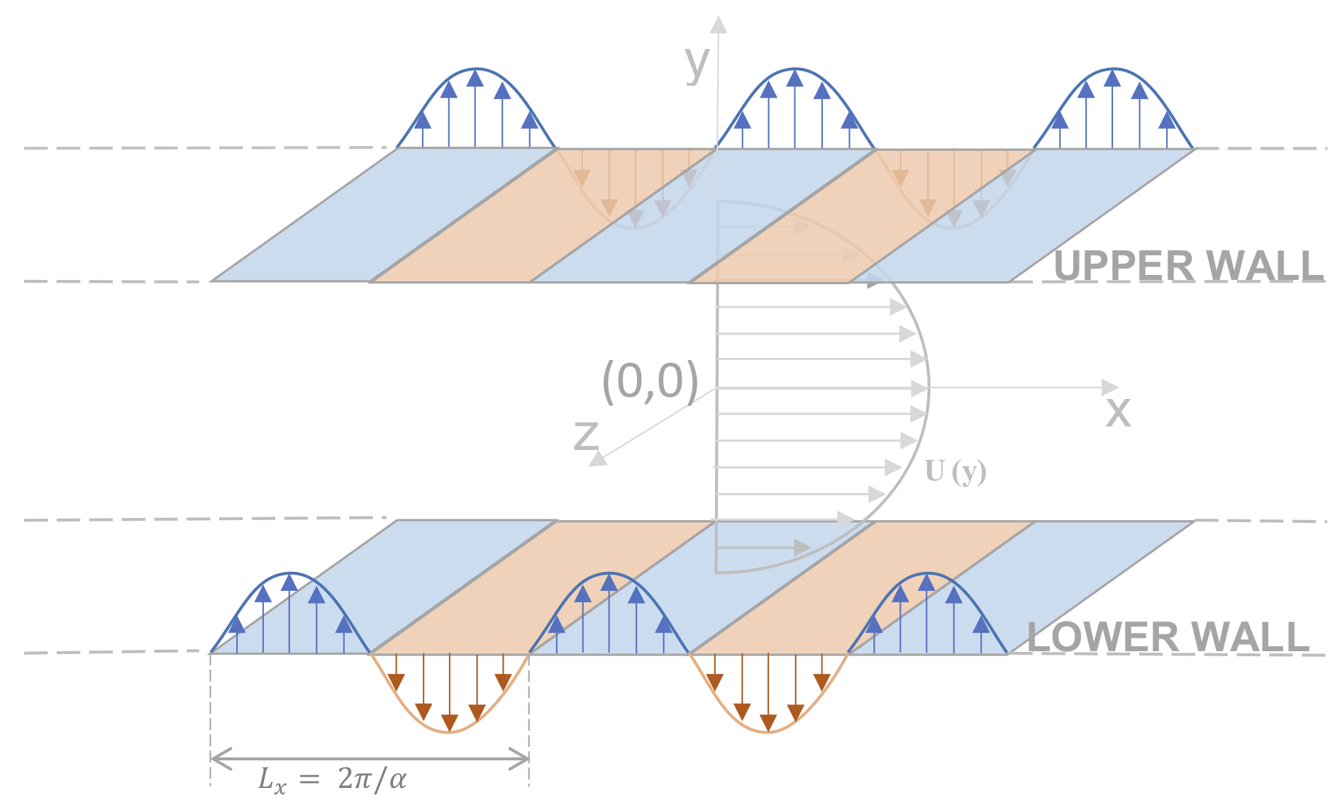
Figure 1: Channel flow setup.

One of the stages to bypass transition within the channel flow setting is the transient energy growth (TEG) of flow perturbations about the base-flow due to non-modal effects [1]. In accordance with previous studies, we use the kinetic energy density as a measure of this TEG,

$$E(t)=\frac{1}{V}\int_{V}\rho\frac{{u}^{2}+v^{2}+w^{2}}{2}dV\leavevmode\nobreak\ ,$$ (11)

where $\rho$ is the fluid density and $V$ is the volume of a unit streamwise length of channel. In relation to earlier discussions, the kinetic energy density can be re-expressed as $E(t):=\mathbf{x}^{T}Q\mathbf{x}$, where $Q=Q^{T}>0$ [35, 36].

In order to implement flow control, we introduce wall-normal blowing and suction actuation at the upper- and lower-walls—consistent with prior investigations on controlling channel flow [13, 15, 8]. Following the modeling procedure in [35], this can be modeled via the wall-transpiration boundary conditions $\tilde{v}(y=1)=q_{u}$, $\tilde{v}(y=-1)=q_{l}$, $\frac{\partial\tilde{v}}{\partial y}\mid_{y=\pm 1}=0$. Here, $q_{u}$ and $q_{l}$ are wall-normal velocities at the upper- and lower-wall, respectively. The final system formulation uses $\dot{q}_{u}$ and $\dot{q}_{l}$ as the control inputs, while reclassifying $q_{u}$ and $q_{l}$ as system states. This introduces two integrators—associated with the controls—within the system model. Finally, the actuated channel flow system can be expressed in state-space form, as in (1), with the state vector defined as $\mathbf{x}=(a_{v_{0}},\dots,a_{v_{N}},a_{\eta_{0}},\dots,a_{\eta_{N}},q_{u},q_{l})^{T}$ and the input vector defined as $\mathbf{u}=(\dot{q}_{u},\dot{q}_{l})^{T}$. It must be noted that the resulting system here is complex-valued, owing to the introduction of Fourier transformations in the streamwise and spanwise directions. As such, a final step is needed to transform the system into an equivalent real-valued state-space realization. Further modeling details can be found in [35].

In the remainder, we consider this linearized channel flow model at a sub-critical Reynolds number of $Re=3000$ (unless otherwise stated) for three different wavenumber pairs $(\alpha,\beta)$: $(1,0)$, $(1,1)$, and $(0,2)$. In all cases, the number of collocation points $N$ is chosen so that the resulting state dimension is $n=199$. The optimal spanwise disturbance to the uncontrolled system with $(\alpha,\beta)=(0,2)$ yields the largest MTEG among all other streamwise, spanwise, and oblique wavenumber configurations. Hence, this spanwise disturbance is an important case to study for controller performance evaluation; The other two wavenumber pairs considered here have also been widely studied in the literature [13, 14].

3.2 Frequency analysis of control-oriented reduced-order models for the channel flow system

Here, we examine how the control-oriented ROMs introduced in Section 2.1 approximate the dynamics of the full-order model (FOM) for the linearized channel flow system, for which $n=199$. Specifically, we examine whether the ROMs developed here capture the input-output behavior of the FOM accurately. In multi-input multi-output (MIMO) systems, the singular values $\sigma$ of the system’s transfer function over various frequencies provide a means of characterizing the input-output behavior of the system. The singular values provide information on the variation in the system’s principal gains in any of the $p$ input direction [37]. Here, we investigate these characteristics as a function of ROM order $r$ from the input $\dot{q}_{u}$ to the flow-state (see Figure 2). In this work, the scaled frequency is given by $f^{*}=ftU_{cl}/h$. The frequency response data reveal that increasing the order $r$ of the ROM decreases the approximation error with respect to the FOM response. Indeed, the trend is more clear from Table 2, which summarizes the root mean square error (RMSE) between the ROM and FOM frequency responses. The acceptable accuracy of a ROM in approximating a FOM response is mostly application specific. For the case here, the RMSE metric suggests that ROMs of $r\geq 20$ perform moderately well. Further, even using the higher-order $r=50$ models—which reflect excellent agreement with the FOM frequency-response—will make LMI-based controller synthesis tractable. The transfer function from input channel $\dot{q}_{l}$ to the flow-state exhibits similar convergence in the frequency-response.

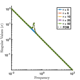
(a) $\alpha=1,\leavevmode\nobreak\ \beta=0$

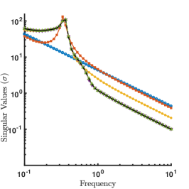
(b) $\alpha=1,\leavevmode\nobreak\ \beta=1$

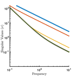
(c) $\alpha=0,\leavevmode\nobreak\ \beta=2$

Figure 2: Frequency response from $\dot{q}_{u}$ to the flow-state at $Re=3000$.

	$r=5$	$r=6$	$r=10$	$r=20$	$r=50$
$\alpha=1,\beta=0$	1.079	0.049	0.0033	$1.340\times 10^{-4}$	$5.726\times 10^{-6}$
$\alpha=1,\beta=1$	18.765	14.135	2.990	0.0891	$9.603\times 10^{-5}$
$\alpha=0,\beta=2$	119.19	61.0560	13.332	1.705	0.0193

Table 2: RMSE between the frequency-response of the FOM ($n=199$) and the ROM of order $r$ at $Re=3000$.

Finally, it should be noted that, for the ROMs presented here, the data-sampling parameters $t_{f}$ and $\delta_{t}$ in the snapshot POD stage of the ROM-procedure were tuned to ensure convergence of the ROM response to the FOM response. In the $Re=3000$ setting, for streamwise waves and oblique waves $\delta_{t}=0.01$ and $t_{f}=30\leavevmode\nobreak\ \text{and}\leavevmode\nobreak\ 50$ respectively. While for spanwise waves we use $\delta_{t}=1$ and $t_{f}=500$ to obtain adequate models. All times reported in this work are non-dimensionalized, and correspond to non-dimensional convective time units $\frac{tU_{cl}}{h}$.

3.3 Controller performance

The synthesis of MTEG-minimizing controllers via the solution of the LMI-problem in (5) is enabled by the control-oriented ROMs reported in Section 3.2 above. The resulting controllers will be referred to as LMI-ROM controllers here. For benchmarking, we compare MTEG performance with two sets of LQR controllers—one designed based on the FOM (“LQR-FOM”) and one designed based on the same ROM that was used for the LMI-based synthesis (“LQR-ROM”). Additionally, since the MTEG-minimizing controller in the LMI-ROM was designed without constraining the control input, we relax the penalty on the input effort within the LQR cost function in (3) by setting $R=10^{-6}I$, where $I$ denotes the identity matrix. This is done in an effort to make a fair comparison between the LMI-ROM, LQR-ROM, and LQR-FOM controllers. Note, this differs from the approach taken in [13], in which a constrained version of the controller was implemented. All controllers are applied to the full-order channel flow model described in Section 3.1 above, then compared based on the MTEG $\Theta_{\text{max}}$ for each respective closed-loop system. In general, the optimal perturbation will differ between each closed-loop system, and will also differ from that of the uncontrolled system. Here we use the optimal perturbation of the respective closed-loop system to perform MTEG analysis. In this study, each optimal perturbation is calculated using the algorithm presented in [38].

As shown in Figure 3, the LMI-ROM controller reduces the MTEG in the system relative to each of the LQR-based controllers for each of the wavenumber pairs considered. For $(\alpha,\beta)=(1,0)$, the LMI-ROM controller reduces $\Theta_{\text{max}}$ by a factor of $\approx 1.88$ in comparison with the LQR controllers (see Figure 3a). Similarly, the LMI-ROM reduces MTEG by a factor of $\approx 2.6$ relative to the LQR controllers for $(\alpha,\beta)=(1,1)$ (see Figure 3b). Finally, for $(\alpha,\beta)=(0,2)$, the difference in MTEG reduction between the LMI-ROM controller and the LQR controllers is only marginally greater (See Figure 3c). This result is consistent with the findings in [13], for which wall-normal blowing/suction was found to be less effective for TEG control than spanwise blowing/suction at the walls. For all controllers and all wavenumber pairs considered here, MTEG was reduced relative to the uncontrolled flow. These results are summarized in Table 3.

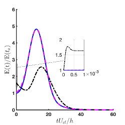
(a) $\alpha=1,\beta=0$ with $r=40$.

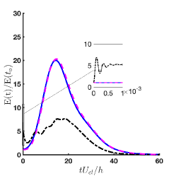
(b) $\alpha=1,\beta=1$ with $r=58$

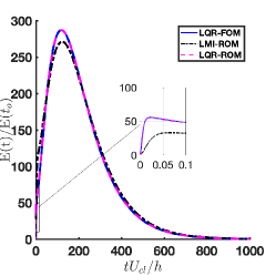
(c) $\alpha=0,\beta=2$ with $r=40$

Figure 3: Worst-case closed-loop TEG responses at $Re=3000$.

		$\Theta_{\text{max}}$
	r	Uncontrolled	LMI-ROM	LQR-FOM	LQR-ROM
$\alpha=1,\beta=0$	40	20.31	2.56	4.81	4.81
$\alpha=1,\beta=1$	58	107.00	7.58	20	20.28
$\alpha=0,\beta=2$	40	1762	271.2	287.1	287.1

Table 3: MTEG $\Theta_{\text{max}}$ for the uncontrolled and controlled channel flow system at $Re=3000$.

Although the LMI-ROM controller outperforms both of the LQR controllers in reducing the MTEG ($\Theta_{\text{max}}$) in the results above, these results depend on the order $r$ of the ROM used for controller synthesis. To investigate this influence, we vary $r$ in the ROM design, then study controller performance on the FOM for streamwise and oblique waves—$(1,0)$ and $(1,1)$, respectively—still with $Re=3000$. We only report values of $r$ for which the open-loop ROMs successfully converge to the FOM dynamics, and so do not consider $r$ smaller than these values here. Figure 4 shows that $\Theta_{\text{max}}$ decreases with increasing ROM order $r$ using the LMI-ROM controller. The same is true for the LQR-ROM controller, but the convergence is more rapid. MTEG for the LQR-ROM converges to that of the LQR-FOM for $r=20$ for streamwise and spanwise waves, and for $r=25$ for oblique waves. We found that for streamwise and oblique wavenumber pairs considered, there exists a ROM order $r$ such that the LMI-ROM controller will outperform both of the LQR controllers for MTEG reduction. We note that although the LMI-ROM yields a reduction in MTEG relative to both LQR-based controllers in the spanwise wave case, this case was also found to be relatively insensitive to the ROM order. Again, this finding is consistent with the results reported in [13], which found that spanwise blowing/suction actuation was required to achieve meaningful reductions in MTEG. Since the current investigation is focused on control-oriented ROM, we continue to focus on wall-normal blowing/suction actuation. Lastly, note that the fact that the LMI-ROM requires a larger $r$ than the LQR-ROM for MTEG performance to converge is to be expected; TEG is a phenomenon intimately related to $\dot{E}(t)$, whose approximation requires higher-precision estimates of $E(t)$.

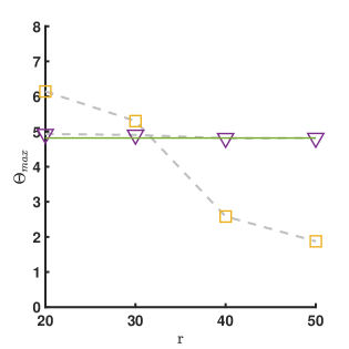
(a) $\alpha=1,\beta=0$.

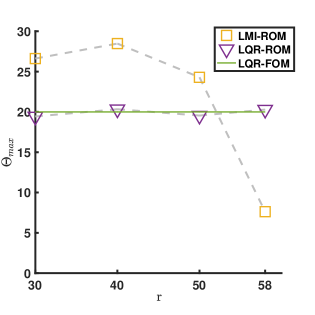
(b) $\alpha=1,\beta=1$

Figure 4: Closed-loop MTEG $\Theta_{\text{max}}$ as a function of ROM order $r$ at $Re=3000$.

It is clear that the LMI-ROM controller in the above cases outperforms both of the LQR controllers. In order to investigate this further, we proceed to analyze the details of the wall-normal actuation and its influence on the flow perturbations. Figure 5 shows the actuated wall-normal velocity at the upper- and lower-walls—$q_{u}$ and $q_{l}$, respectively—for each controller. The case of $(\alpha,\beta)=(1,0)$, shown in Figure 5a, reveals that LMI-ROM controller results in blowing and suction at the upper- and lower-walls that are equal in magnitude, but opposite in direction. In contrast, each of the LQR-ROM and the LQR-FOM controllers produces almost identical (both in magnitude and direction) blowing and suction at the upper- and lower-walls. Interestingly, the LQR-ROM controls differ from the LQR-FOM controls for a short period at the beginning of the response, which is an expected artifact of the modal truncation. The 5% settling time on the actuation for the LMI-ROM controllers is  $\approx 43$ convective time units; the LQR controllers settle in $\approx 34$ convective time units, indicating a shorter duration of control.

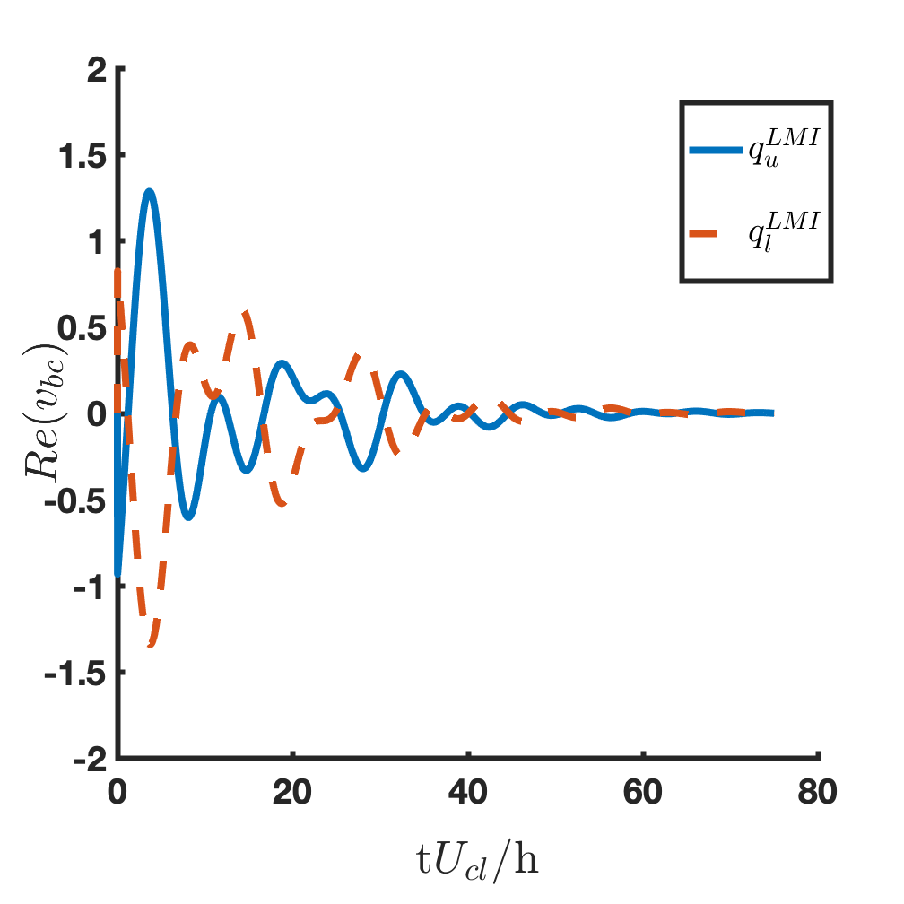
(a) LMI-ROM control

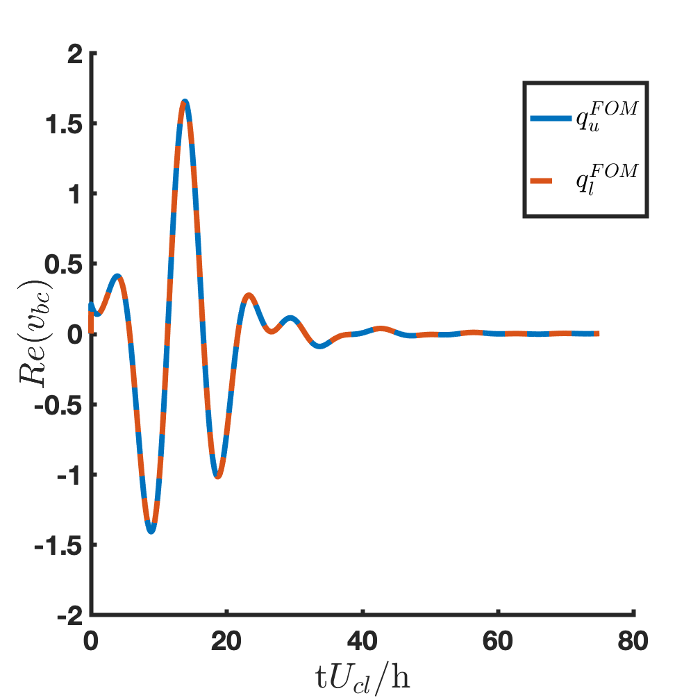
(b) LQR-FOM control

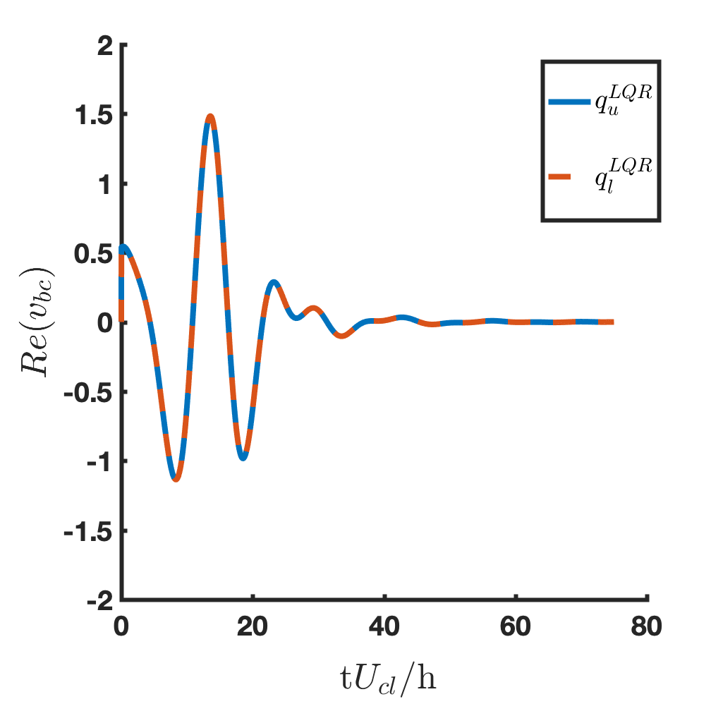
(c) LQR-ROM control

Figure 5: Actuated wall-normal velocity for $r=40$, $(\alpha,\beta)=(1,0)$, and $Re=3000$.

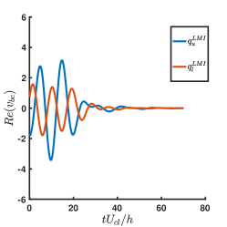
(a) LMI-ROM control

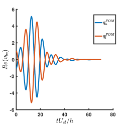
(b) LQR-FOM control

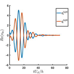
(c) LQR-ROM control

Figure 6: Actuated wall-normal velocity for $r=58$, $(\alpha,\beta)=(1,1)$, and $Re=3000$.

In the oblique wave case of $(\alpha,\beta)=(1,1)$, shown in Figure 6a, the LMI-ROM controller results in a maximum wall-normal blowing/suction velocity that is $\approx 1.6$ times lower than either of the LQR controllers. From Figure 6a we find that the $q_{u}$ produces a control input of larger magnitude compared to $q_{l}$, i.e., the actuator on the upper-wall is inducing a larger velocity compared to the actuator on the lower-wall. In Figures 6b and 6c the upper-wall and lower-wall actuators produce a velocity of similar magnitude, but opposite directions relative to each other. In the oblique wave case, the $5\%$ settling time of the actuation signal for the LMI-ROM controller is $\approx 41$ convective time units, while the LQR-FOM and LQR-ROM each have a settling time of $\approx 37$ convective time units. In the spanwise waves setting, shown in Figure 7, the LMI-ROM controller actuates the system similarly to both of the LQR controllers, but with a lower initial magnitude. For all controllers, wall-normal transpiration at the upper-wall is identical to that at the lower-wall (see Figure 7).

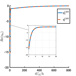
(a) LMI-ROM control

(b) LQR-FOM control

(c) LQR-ROM control

Figure 7: Actuated wall-normal velocity for $r=40$, $(\alpha,\beta)=(0,2)$, and $Re=3000$.

Next, we examine the evolution of perturbations in streamwise velocity ($u$) to analyze the effect of the different controllers on the flow response. Figures 8 – 10 show the evolution of normalized $u$ perturbations. In these figures, the initial optimal perturbation has been normalized such that $E(0)=1$. Figure 8 shows the response for the case of streamwise waves. Note that the LMI-ROM controller has a streamwise perturbation profile different from that of the LQR-ROM and the LQR-FOM. The $u$ perturbations die out faster with the LMI-ROM controller than with either of the LQR controllers. The LQR-FOM and the LQR-ROM result in a similar evolution of $u$ perturbation, as is to be expected from the similarity in TEG profiles we noted earlier in Figure 3a. In the case of oblique waves (see Figure 9), the LQR-ROM and LQR-FOM again yield a similar response in $u$-perturbations. In contrast to these responses, the LMI-ROM controller results in a reduced magnitude of $u$ at the lower walls of the channel. Again, the LMI-ROM results in a faster decay of $u$ perturbations than the LQR-ROM and LQR-FOM controllers. Finally, in the case of spanwise waves (see Figure 10), all the three controllers yield similar responses in $u$.

(a) LMI-ROM control

(b) LQR-FOM control

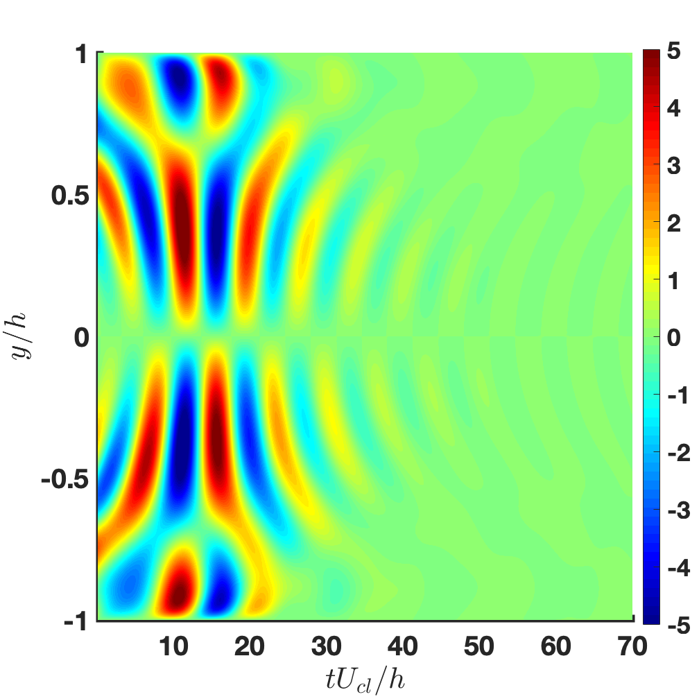
(c) LQR-ROM control

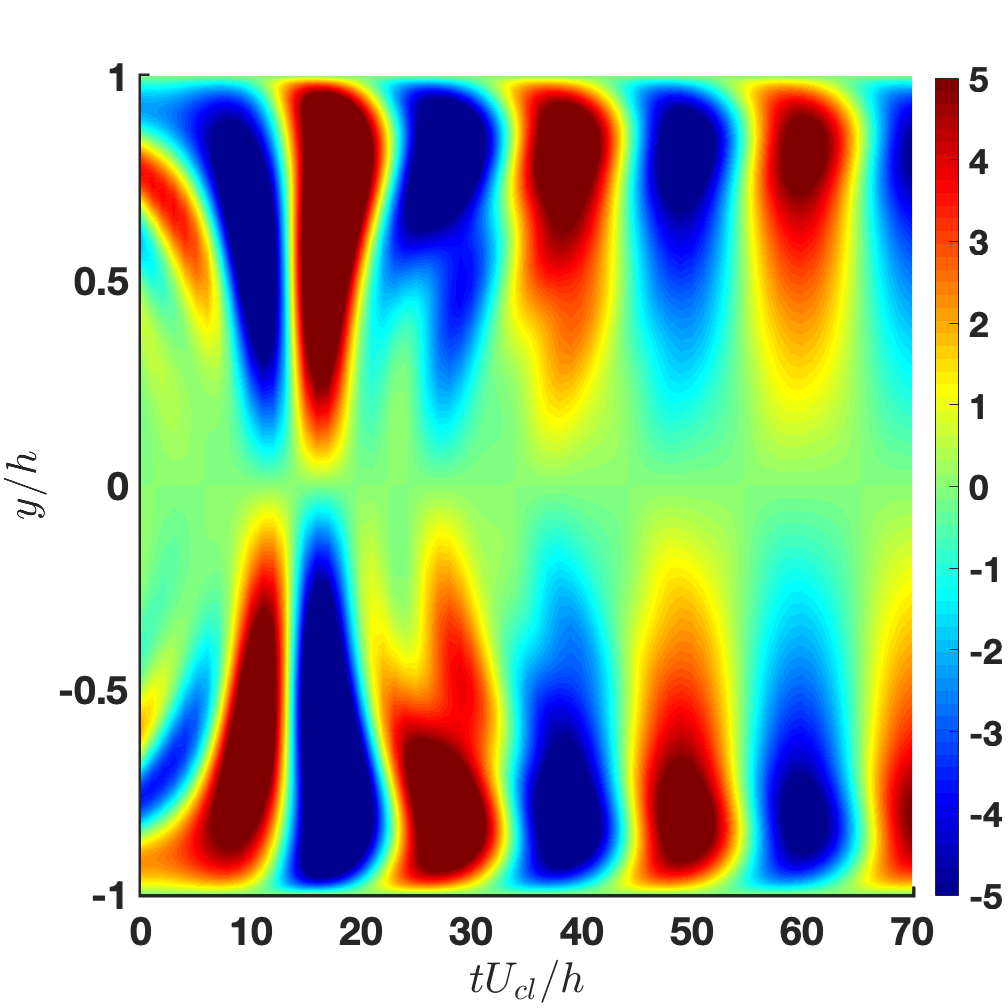
(d) Uncontrolled

Figure 8: Evolution of streamwise velocity perturbations ($u$) for $r=40$, $(\alpha,\beta)=(1,0)$, and $Re=3000$.

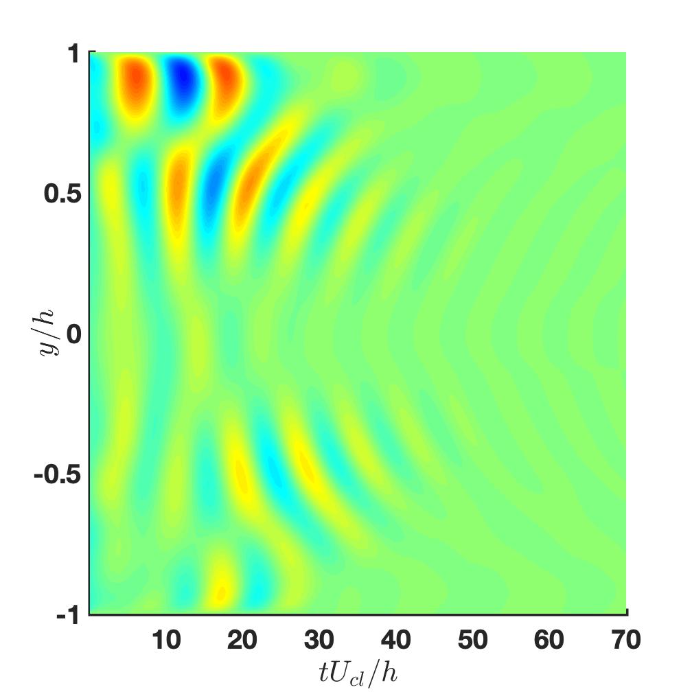
(a) LMI-ROM control

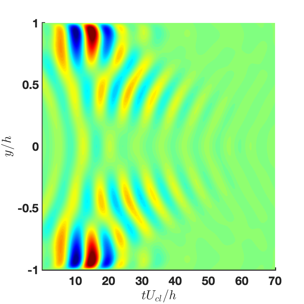
(b) LQR-FOM control

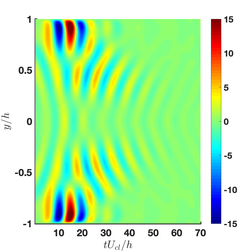
(c) LQR-ROM control

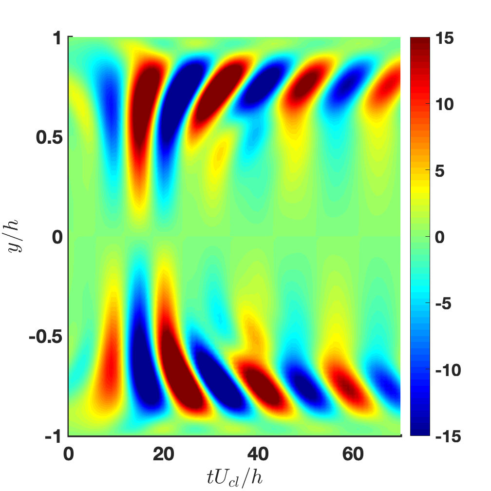
(d) Uncontrolled

Figure 9: Evolution of streamwise velocity perturbations ($u$) for $r=58$, $(\alpha,\beta)=(1,1)$, and $Re=3000$.

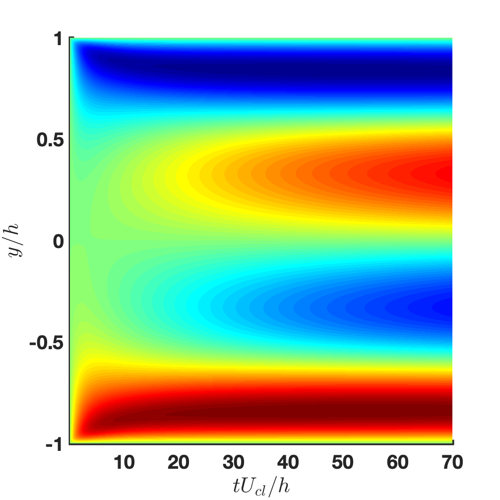
(a) LMI-ROM control

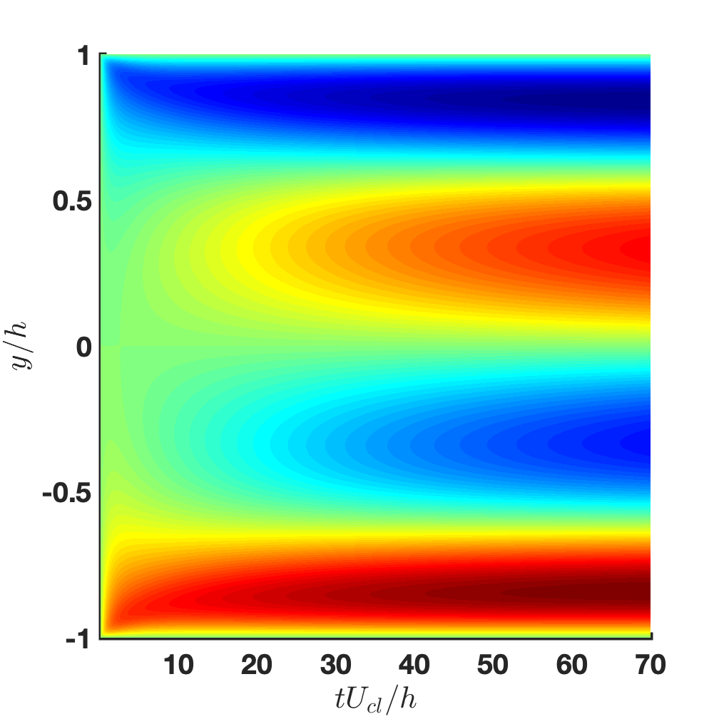
(b) LQR-FOM control

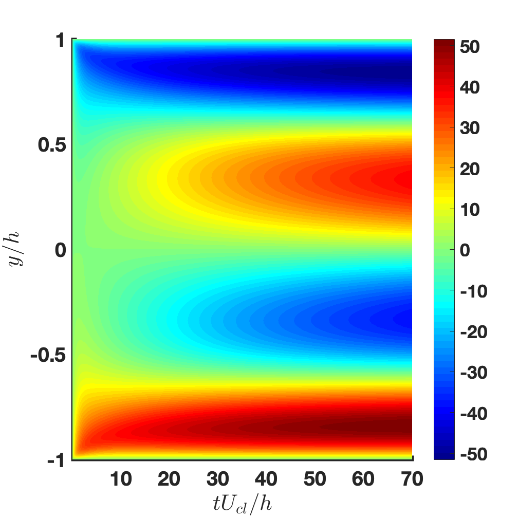
(c) LQR-ROM control

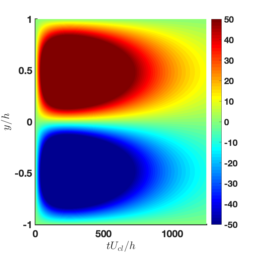
(d) Uncontrolled

Figure 10: Evolution of streamwise velocity perturbations ($u$) for $r=40$, $(\alpha,\beta)=(0,2)$, and $Re=3000$.

Finally, we repeat our study for other $Re$ values to ensure that the ROMs and controllers can be used in other settings as well. ROMs are developed and tuned to converge for $Re=1000$, $5000$, and $10,000$. Then, we follow the same procedure for control synthesis as in the $Re=3000$ cases described earlier. Note that for the case of $Re=10,000$, the flow is linearly unstable; thus, the balanced truncation procedure for the model reduction is only performed on the stable subspace of the linearized dynamics. Figures 11 and 12 report performance results for the cases of $(\alpha,\beta)=(1,0)$ and $(1,1)$, respectively. The results clearly show that the LMI-ROM controllers reduce TEG to a greater extent than the LQR controllers. However, with the increase in $Re$, the closed-loop response to the LMI-ROM control exhibits oscillations on a transient time scale, on the order of of approximately $10^{-2}\leavevmode\nobreak\ \text{to}\leavevmode\nobreak\ 10^{-4}$ convective time units. The transient oscillations appear to be a property of the closed-loop system, which has a set of eigenvalues with large imaginary parts—on the order of $10^{4}$—that lead to lightly damped oscillations. Further investigation is necessary to determine the underlying cause of these transient oscillations and the observed spectral properties of the closed-loop system.

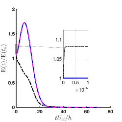
(a) $Re=1000$ ($r=40$)

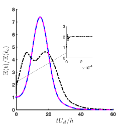
(b) $Re=5000$ ($r=50$)

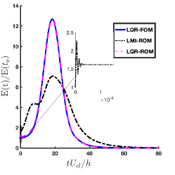
(c) $Re=10,000$ ($r=58$)

Figure 11: Worst-case closed-loop TEG responses for $(\alpha,\beta)=(1,0)$.

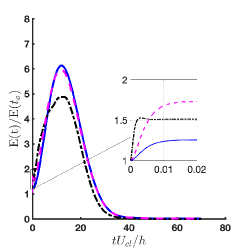
(a) $Re=1000$ ($r=40$)

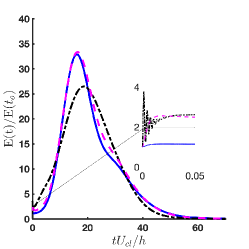
(b) $Re=5000$ ($r=58$)

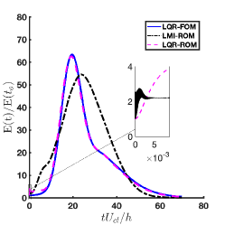
(c) $Re=10,000$ ($r=58$)

Figure 12: Worst-case closed-loop TEG responses for $(\alpha,\beta)=(1,1)$.

4 Conclusions

In this paper, we have investigated the use of control-oriented ROMs for designing feedback controllers that minimize the MTEG of flow perturbations within a linearized channel flow. The ROMs were formed using an output projection onto POD modes, followed by a balanced truncation procedure to reduce the state dimension. POD modes were chosen in order to best approximate the perturbation energy, as needed for representing the objective function for control. Note that this output projection does not alter the state dimension of the system. As such, a balanced truncation was performed to reduce the state dimension, retaining only state variables that were essential to preserving the system’s input-output dynamics. ROMs of the linearized channel flow system enabled the synthesis of MTEG-minimizing controllers through the solution of an LMI problem that would otherwise have been computationally prohibitive. Specifically, the dimension of the full-order model ($n=199$) was reduced to yield ROMs with order $r=40-60$, depending on the specific configuration. This constitutes a significant reduction in the computational demand for the subsequent LMI-based controller synthesis, since the computational requirements for LMI-based controller synthesis scale as $\mathcal{O}(n^{6})$. Further, the MTEG-minimizing controllers designed using the proposed ROMs were found to outperform LQR controllers in suppressing TEG, even when these LQR controllers were designed based on the full-order system model. Although not explicitly reported here, the present investigation revealed that ROM-based MTEG-minimizing controllers can be sensitive to $Re$ variations, leading to linearly unstable closed-loop systems when applied in “off-design” settings. As such, future investigations will need to focus on addressing these fragilities. It is expected that both the model reduction and controller synthesis approaches will need to be re-formulated to robustly minimize MTEG.

5 Acknowledgements

This material is based upon work supported by the Air Force Office of Scientific Research under award numbers FA9550-17-1-0252 and FA9550-19-0034, monitored by Drs. Douglas R. Smith and Gregg Abate.

Appendix A Limitations of Modal truncation for MTEG-minimizing control

Modal truncation based on the eigendecomposition of the matrix $A=V\Lambda V^{-1}$ in (1) is a common approach for reduced-order modeling, primarily owing to its simplicity. Since the eigenvalues $\lambda_{i}$ in the diagonal matrix $\Lambda$ provide information about the relative time-scales of the modal response, a simple strategy for modal truncation is to omit modes using time-scale arguments. For example, when long term behavior is of interest, then modes with fast decay rates and/or high oscillation frequencies can be omitted. ROMs constructed time-scale based modal truncation will not necessarily capture the input-output dynamics needed for controller synthesis. Thus, another common approach considers a measure of modal controllability/observability, given by the ratio [30]

$$\zeta_{i}=\frac{\|C_{i}\|\|B_{i}\|}{|\mathrm{Re}\{\lambda_{i}\}|},$$ (12)

where $B_{i}$ and $C_{i}$ correspond to the $i^{\text{th}}$ row and column of the modal representations of the matrices $B$ and $C$ from (1), respectively. Modes with larger values of $\zeta_{i}$ contribute more to the input-output dynamics and should be be retained, whereas those with lower values of $\zeta_{i}$ can be truncated.

Here, we apply both of these modal truncation approaches to arrive at ROMs with order $r<n$ of the linearized channel flow system with $(\alpha,\beta)=(1,0)$ and $Re=3000$. For truncation modal truncation by time-scale arguments, we truncate the “fastest” modes (i.e., stable modes with relatively large $|\mathrm{Re}\{\lambda_{i}\}|$). For truncation by modal controllability/observability, we truncate the least controllable/observable modes (i.e., stable modes with relatively small $\zeta_{i}$). Each of these ROMs is then used to design the LMI-ROM and LQR-ROM controllers. The resulting performance of each of these controllers is compared with the LQR-FOM controller in Figure 13. The model orders here were chosen based on convergence of the ROM open-loop frequency-response relative to the FOM. We note that for the results reported in the Appendix here, the FOM dimension is set to $n=99$; without doing so, ROMs based on modal truncation converge with $r>80$, which makes the LMI-based synthesis procedure intractable with the available computational resources. Figure 14 reports the resulting MTEG $\Theta_{\text{max}}$ as a function of $r$ for ROMs constructed by each of the modal truncation approaches. Interestingly, the truncation of “fast modes” yields improved MTEG performance with the LMI-ROM than truncation based on $\zeta_{i}$. These results indicate that modal truncation is a poor candidate for designing controllers to reduce TEG. Although in some cases these models can result in effective control laws, the model orders tend to be higher than the tailored approaches considered in this study. The short-comings of modal truncation—and other ROM methods—for TEG reduction further motivates the need for control-oriented model reduction, like the approach presented in Section 2.1.

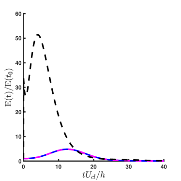
(a) $|\mathrm{Re}\{\lambda_{i}\}|$ modal truncation ($r=50$)

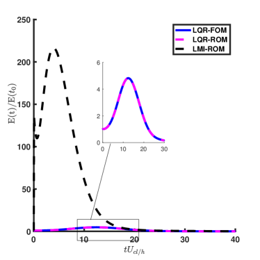
(b) $\zeta_{i}$ modal truncation ($r=50$)

Figure 13: Worst-case closed-loop TEG response for $(\alpha,\beta)=(1,0)$ and $Re=3000$.

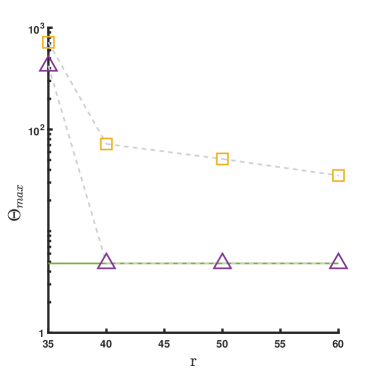
(a) $|\mathrm{Re}\{\lambda_{i}\}|$ modal truncation

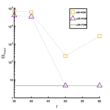
(b) $\zeta_{i}$ modal truncation

Figure 14: Closed-loop MTEG $\Theta_{\text{max}}$ as a function of ROM order $r$ for $(\alpha,\beta)=(1,0)$ at $Re=3000$.

References

- Schmid and Henningson [2001] Schmid, P. J., and Henningson, D. S., Stability and transition in shear flows, Springer, 2001. 10.1115/1.1470687.
- Patel and Head [1969] Patel, V. C., and Head, M. R., “Some observations on skin friction and velocity profiles in fully developed pipe and channel flows,” Journal of Fluid Mechanics, Vol. 38, No. 1, 1969, pp. 181–201. 10.1017/S0022112069000115.
- Reddy and Henningson [1993] Reddy, S. C., and Henningson, D. S., “Energy growth in viscous channel flows,” Journal of Fluid Mechanics, Vol. 252, No. -1, 1993, p. 209. 10.1017/S0022112093003738.
- Trefethen et al. [1993] Trefethen, L. N., Trefethen, A. E., Reddy, S. C., and Driscoll, T. A., “Hydrodynamic stability without eigenvalues.” Science (New York, N.Y.), Vol. 261, No. 5121, 1993, pp. 578–84. 10.1126/science.261.5121.578.
- Henningson and Reddy [1994] Henningson, D. S., and Reddy, S. C., “On the role of linear mechanisms in transition to turbulence,” Physics of Fluids, Vol. 6, No. 3, 1994, pp. 1396–1398. 10.1063/1.868251.
- Schmid [2007] Schmid, P. J., “Nonmodal Stability Theory,” Annual Review of Fluid Mechanics, Vol. 39, 2007, pp. 129–62. 10.1146/annurev.fluid.38.050304.092139.
- Chapman [2002] Chapman, S. J., “Subcritical transition in channel flows,” Journal of Fluid Mechanics, Vol. 451, 2002, pp. 35–97. 10.1017/S0022112001006255.
- Bewley [2001] Bewley, T. R., “Flow control: New challenges for a new Renaissance,” Progress in Aerospace Sciences, Vol. 37, No. 1, 2001, pp. 21–58. 10.1016/S0376-0421(00)00016-6.
- Bagheri and Henningson [2011] Bagheri, S., and Henningson, D. S., “Transition delay using control theory,” Philosophical Transactions: Mathematical, Physical and Engineering Sciences, Vol. 369, 2011. 10.1098/rsta.2010.0358.
- Kim and Bewley [2007] Kim, J., and Bewley, T. R., “A Linear Systems Approach to Flow Control,” Annual Review of Fluid Mechanics, Vol. 39, No. 1, 2007, pp. 383–417. 10.1146/annurev.fluid.39.050905.110153.
- Bewley and Liu [2018] Bewley, T. R., and Liu, S., “Optimal and robust control and estimation of linear paths to transition,” Journal of Fluid Mechanics, Vol. 365, 2018, pp. 305–349. 10.1017/S0022112098001281.
- Ilak and Rowley [2008a] Ilak, M., and Rowley, C. W., “Feedback Control of Transitional Channel Flow using Balanced Proper Orthogonal Decomposition,” AIAA Theoretical Fluid Mechanics Conference, Seattle, WA, AIAA paper 2008-4230, 2008a.
- Martinelli et al. [2011] Martinelli, F., Quadrio, M., Mckernan, J., and Whidborne, J. F., “Linear feedback control of transient energy growth and control performance limitations in subcritical plane Poiseuille flow,” Physics of Fluids, 2011. 10.1063/1.3540672.
- Hogberg et al. [2003] Hogberg, M., Bewley, T. R., and Henningson, D. S., “Linear feedback control and estimation of transition in plane channel flow,” Journal of Fluid Mechanics, Vol. 481, 2003, pp. 149–175. 10.1017/S0022112003003823.
- Joshi et al. [1999] Joshi, S. S., Speyer, J. L., and Kim, J., “Finite Dimensional Optimal Control of Poiseuille Flow,” Journal of Guidance, Control, and Dynamics, Vol. 22, No. 2, 1999. 10.2514/2.4383.
- Hemati and Yao [2018] Hemati, M. S., and Yao, H., “Performance Limitations of Observer-Based Feedback for Transient Energy Growth Suppression,” AIAA Journal, 2018. 10.2514/1.j056877.
- Yao and Hemati [2018] Yao, H., and Hemati, M. S., “Revisiting the separation principle for improved transition control,” AIAA Paper 2018-3693, 2018. 10.2514/6.2018-3693.
- Yao and Hemati [2019] Yao, H., and Hemati, M. S., “Advances in Output Feedback Control of Transient Energy Growth in a Linearized Channel Flow,” AIAA Paper 2019-0882, 2019. 10.2514/6.2019-0882.
- Whidborne and McKernan [2007] Whidborne, J. F., and McKernan, J., “On the Minimization of Maximum Transient Energy Growth,” IEEE Transactions on Automatic Control, Vol. 52, No. 9, 2007, pp. 1762–1767. 10.1109/TAC.2007.900854.
- Butler and Farrell [1992] Butler, K. M., and Farrell, B. F., “Three-dimensional optimal perturbations in viscous shear flow,” Physics of Fluids A: Fluid Dynamics, Vol. 4, No. 8, 1992, pp. 1637–1650. 10.1063/1.858386.
- Jovanovic and Bameih [2005] Jovanovic, M. R., and Bameih, B., “Componentwise energy amplification in channel flows,” Journal of Fluid Mechanics, Vol. 534, 2005, p. 145–183. 10.1017/S0022112005004295.
- Boyd et al. [1994] Boyd, S., El Ghaoui, L., Feron, E., and Balakrishnan, V., Linear Matrix Inequalities in System and Control Theory, Society for Industrial and Applied Mathematics, 1994. 10.1137/1.9781611970777.
- Barbagallo et al. [2012] Barbagallo, A., Sipp, D., and Schmid, P. J., “Reduced Order Models for Closed Loop Control: Comparison between POD, BPOD, and Global Modes,” Progress in Flight Physics, Vol. 3, 2012, pp. 503–512. 10.1051/eucass/201203503.
- Jones et al. [2015] Jones, B. L., Heins, P. H., Kerrigan, E. C., Morrison, J. F., and Sharma, A. S., “Modelling for robust feedback control of fluid flows,” Journal of Fluid Mechanics, Vol. 769, 2015, pp. 687–722. 10.1017/jfm.2015.84.
- Taira et al. [2017] Taira, K., Brunton, S. L., Dawson, S. T. M., Rowley, C. W., Colonius, T., Mckeon, B. J., Schmidt, O. T., Gordeyev, S., Theofilis, V., and Ukeiley, L. S., “Modal Analysis of Fluid Flows: An Overview,” AIAA Journal, 2017. 10.2514/1.J056060.
- Rowley and Dawson [2017] Rowley, C. W., and Dawson, S. T. M., “Model Reduction for Flow Analysis and Control,” Annual Review of Fluid Mechanics, Vol. 49, 2017, pp. 387–417. 10.1146/annurev-fluid-010816-060042.
- Rowley [2005] Rowley, C. W., “Model reduction for fluids using balanced proper orthogonal decomposition,” International Journal on Bifurcation and Chaos, Vol. 15, No. 3, 2005, pp. 997–1013. 10.1142/S0218127405012429.
- Ilak and Rowley [2008b] Ilak, M., and Rowley, C. W., “Modeling of transitional channel flow using balanced proper orthogonal decomposition,” Physics of Fluids, Vol. 20, 2008b, p. 34103. 10.1063/1.2840197.
- Moore [1981] Moore, B., “Principal component analysis in linear systems: Controllability, observability, and model reduction,” IEEE Transactions on Automatic Control, Vol. 26, No. 1, 1981, pp. 17–32. 10.1109/TAC.1981.1102568.
- Antoulas [2006] Antoulas, A. C., Approximation of Large-Scale Dynamical Systems, Society for Industrial and Applied Mathematics, 2006.
- Willcox and Peraire [2002] Willcox, K., and Peraire, J., “Balanced Model Reduction via the Proper Orthogonal Decomposition,” AIAA Journal, Vol. 40, No. 11, 2002. 10.2514/2.1570.
- Grant and Boyd [2014] Grant, M., and Boyd, S., “CVX: Matlab Software for Disciplined Convex Programming, version 2.1,” http://cvxr.com/cvx, Mar. 2014.
- Laub et al. [1987] Laub, A. J., Heath, M. T., Paige, C. C., and Ward, R. C., “Computation of System Balancing Transformations and Other Applications of Simultaneous Diagonalization Algorithms,” IEEE Transactions on Automatic Control, Vol. AC-32, No. 2, 1987, pp. 115–122. 10.1109/TAC.1987.1104549.
- Boyd [2000] Boyd, J. P., Chebyshev and Fourier Spectral Methods, Dover Publications, 2000. 10.1007/978-0-387-77674-3.
- McKernan et al. [2006] McKernan, J., Papadakis, G., and Whidborne, J. F., “A linear state-space representation of plane Poiseuille flow for control design: a tutorial,” International Journal of Modelling, Identification and Control, Vol. 1, No. 4, 2006, p. 272. 10.1504/IJMIC.2006.012615.
- McKernan [2006] McKernan, J., “Control of Plane Poiseuille Flow: A Theoretical and Computational Investigation,” Ph.D. thesis, Cranfield University, 2006.
- Skogestad and Postlethwaite [2005] Skogestad, S., and Postlethwaite, I., Multivariable feedback control : analysis and design, John Wiley, 2005.
- Whidborne and Amar [2011] Whidborne, J. F., and Amar, N., “Computing the maximum transient energy growth,” BIT Numerical Mathematics, Vol. 51, No. 2, 2011, pp. 447–457. 10.1007/s10543-011-0326-4.