Selecting the independent coordinates of manifolds with large aspect ratios

Abstract

Many manifold embedding algorithms fail apparently when the data manifold has a large aspect ratio (such as a long, thin strip). Here, we formulate success and failure in terms of finding a smooth embedding, showing also that the problem is pervasive and more complex than previously recognized. Mathematically, success is possible under very broad conditions, provided that embedding is done by carefully selected eigenfunctions of the Laplace-Beltrami operator $\Delta$. Hence, we propose a bicriterial Independent Eigencoordinate Selection (IES) algorithm that selects smooth embeddings with few eigenvectors. The algorithm is grounded in theory, has low computational overhead, and is successful on synthetic and large real data.

1 Motivation

We study a well-documented deficiency of manifold learning algorithms. Namely, as shown in [GZKR08], algorithms that find their output $\mathbf{\bm{Y}}=\varphi(\mathbf{\bm{X}})$ by minimizing a quadratic form under some normalization constraints, fail spectacularly when the data manifold has a large aspect ratio, that is, it extends much more in one direction than in others, as the long, thin strip illustrated in Figure 1. This class, called output normalized (ON) algorithms, includes Locally Linear Embedding (LLE), Laplacian Eigenmap, Local Tangent Space Alignment (LTSA), Hessian Eigenmaps (HLLE), and Diffusion maps. The problem, often observed in practice, was formalized in [GZKR08] as failure to find an $\mathbf{\bm{Y}}$ affinely equivalent to $\mathbf{\bm{X}}$. They give sufficient conditions for failure, using a linear algebraic perspective. The conditions show that, especially when noise is present, the problem is pervasive.

In the present paper, we revisit the problem from a differential geometric perspective. First, we define failure not as distortion, but as drop in the rank of the mapping $\phi$ represented by the embedding algorithm. In other words, the algorithm fails when the map $\phi$ is not invertible, or, equivalently, when the dimension $\dim\phi(\mathcal{M})<\dim\mathcal{M}=d$, where $\mathcal{M}$ represents the idealized data manifold, and $\dim$ denotes the intrinsic dimension. Figure 1 demonstrates that the problem is fixed by choosing the eigenvectors with care. In fact, as we show in Section 6, it is known [Bat14] that for the DM and LE algorithms, under mild geometric conditions, one can always find a finite set of $m$ eigenfunctions that provide a smooth $d$-dimensional map. We call this problem the Independent Eigencoordinate Selection (IES) problem, formulate it and explain its challenges in Section 3.

Our second main contribution (Section 4) is to design a bicriterial method that will select from a set of coordinate functions $\phi_{1},\ldots\,\phi_{m}$, a subset $S$ of small size that provides a smooth full-dimensional embedding of the data. The IES problem requires searching over a combinatorial number of sets. We show (Section 4) how to drastically reduce the computational burden per set for our algorithm. Third, we analyze the proposed criterion under asymptotic limit (Section 6). Finally (Section 7), we show examples of successful selection on real and synthetic data. The experiments also demonstrate that users of manifold learning for other than toy data must be aware of the IES problem and have tools for handling it. Notations table, proofs, a library of hard examples, extra experiments and analyses are in Supplements A–G; Figure/Table/Equation references with prefix S are in the Supplement.

2 Background on manifold learning

Manifold learning (ML) and intrinsic geometry  Suppose we observe data $\mathbf{\bm{X}}\in{\mathbb{R}}^{n\times D}$, with data points denoted by $\mathbf{\bm{x}}_{i}\in{\mathbb{R}}^{D}~{}\forall~{}i\in[n]$, that are sampled from a smooth $d$-dimensional submanifold $\mathcal{M}\subset{\mathbb{R}}^{D}$. Manifold Learning algorithms map $\mathbf{\bm{x}}_{i},i\in[n]$ to $\mathbf{\bm{y}}_{i}=\phi(\mathbf{\bm{x}}_{i})\in{\mathbb{R}}^{s}$, where $d\leq s\ll D$, thus reducing the dimension of the data $\mathbf{\bm{X}}$ while preserving (some of) its properties. Here we present the LE/DM algorithm, but our results can be applied to other ML methods with slight modification.

The first two steps of LE/DM [CL06, NLCK06] algorithms are generic; they are performed by most ML algorithms. First we encode the neighborhood relations in a neighborhood graph, which is an undirected graph $G(V,E)$ with vertex set $V$ be the collection of all points $i\in[n]$ and edge set $E$ be the collections of tuple $(i,j)\in V^{2}$ such that $i$ is $j$’s neighbor (and vice versa). Common methods for building neighborhood graphs include $r$-radius graph and $k$-nearest neighbor graph. Readers are encouraged to refer to [HAvL07, THJ10] for details. In this paper, $r$-radius graph are considered, for which principled methods to select the neighborhood size and dimension exist. For such method, the edge set $E$ of the neighborhood graph is constructed as follow: $E=\{(i,j)\in V^{2}:\|\mathbf{\bm{x}}_{i}-\mathbf{\bm{x}}_{j}\|_{2}\leq r\}$. Closely related to the neighborhood graph is the kernel matrix $\mathbf{\bm{K}}\in{\mathbb{R}}^{n\times n}$ whose elements are $K_{ij}=\exp\left(-\tfrac{\|\mathbf{\bm{x}}_{i}-\mathbf{\bm{x}}_{j}\|}{\varepsilon^{2}}\right)\;\text{if }(i,j)\in E\text{ and }0\text{ otherwise}$. Typically, the radius $r$ and the bandwidth parameter $\varepsilon$ are related by $r=c\varepsilon$ with $c$ a small constant greater than 1, e.g., $c\in[3,10]$. This ensures that $\mathbf{\bm{K}}$ is close to its limit when $r\rightarrow\infty$ while remaining sparse, with sparsity structure induced by the neighborhood graph. Having obtained the kernel matrix $\mathbf{\bm{K}}$, we then construct the renormalized graph Laplacian matrix $\mathbf{\bm{L}}$ [CL06], also called the sample Laplacian, or Diffusion Maps Laplacian, by the following: $\mathbf{\bm{L}}=\mathbf{\bm{I}}_{n}-\tilde{\mathbf{\bm{W}}}^{-1}\mathbf{\bm{W}}^{-1}\mathbf{\bm{K}}\mathbf{\bm{W}}^{-1},$ where $\mathbf{\bm{W}}=\operatorname{diag}(\mathbf{\bm{K}}\mathbf{\bm{1}}_{n})$ with $\mathbf{\bm{1}}_{n}$ be all one vectors and $\tilde{\mathbf{\bm{W}}}=\operatorname{diag}\left(\mathbf{\bm{W}}^{-1}\mathbf{\bm{K}}\mathbf{\bm{W}}^{-1}\mathbf{\bm{1}}_{n}\right)$. The method of constructing $\mathbf{\bm{L}}$ as described above guarantees that if the data are sampled from a manifold $\mathcal{M}$, $\mathbf{\bm{L}}$ converges to $\Delta_{\mathcal{M}}$ [HAvL05, THJ10]. A summary of the construction of $\mathbf{\bm{L}}$ can be found in Algorithm 5 Laplacian. The last step of LE/DM algorithm embeds the data by solving the minimum eigen-problem of $\mathbf{\bm{L}}$. The desired $m$ dimensional embedding coordinates are obtained from the second to $m+1$-th principal eigenvectors of graph Laplacian $\mathbf{\bm{L}}$, with $0=\lambda_{0}<\lambda_{1}\leq\ldots\leq\lambda_{m}$, i.e., $\mathbf{\bm{y}}_{i}=(\phi_{1}(\mathbf{\bm{x}}_{i}),\ldots\phi_{m}(\mathbf{\bm{x}}_{i}))$ (see also Supplement B).

To analyze ML algorithms, it is useful to consider the limit of the mapping $\phi$ when the data is the entire manifold $\mathcal{M}$. We denote this limit also by $\phi$, and its image by $\phi(\mathcal{M})\in{\mathbb{R}}^{m}$. For standard algorithms such as LE/DM, it is known that this limit exists [CL06, BN07, HAvL05, HAvL07, THJ10]. One of the fundamental requirements of ML is to preserve the neighborhood relations in the original data. In mathematical terms, we require that $\phi:\mathcal{M}\rightarrow\phi(\mathcal{M})$ is a smooth embedding, i.e., that $\phi$ is a smooth function (i.e. does not break existing neighborhood relations) whose Jacobian $\textbf{{D}}\phi(\mathbf{\bm{x}})$ is full rank $d$ at each $\mathbf{\bm{x}}\in\mathcal{M}$ (i.e. does not create new neighborhood relations).

The pushforward Riemannian metric

A smooth $\phi$ does not typically preserve geometric quantities such as distances along curves in $\mathcal{M}$. These concepts are captured by Riemannian geometry, and we additionally assume that $(\mathcal{M},g)$ is a Riemannian manifold, with the metric $g$ induced from ${\mathbb{R}}^{D}$. One can always associate with $\phi(\mathcal{M})$ a Riemannian metric $g_{*\phi}$, called the pushforward Riemannian metric [Lee03], which preserves the geometry of $(\mathcal{M},g)$; $g_{*\phi}$ is defined by

$$\langle\mathbf{\bm{u}},\mathbf{\bm{v}}\rangle_{g_{*\phi}(\mathbf{\bm{x}})}=\left\langle\textbf{{D}}\phi^{-1}(\mathbf{\bm{x}})\mathbf{\bm{u}},\textbf{{D}}\phi^{-1}(\mathbf{\bm{x}})\mathbf{\bm{v}}\right\rangle_{g(\mathbf{\bm{x}})}\text{ for all }\mathbf{\bm{u}},\mathbf{\bm{v}}\in\mathcal{T}_{\phi(\mathbf{\bm{x}})}\phi(\mathcal{M})$$ (1)

In the above, $\mathcal{T}_{\mathbf{\bm{x}}}\mathcal{M}$, $\mathcal{T}_{\phi(\mathbf{\bm{x}})}\phi(\mathcal{M})$ are tangent subspaces, $\textbf{{D}}\phi^{-1}(\mathbf{\bm{x}})$ maps vectors from $\mathcal{T}_{\phi(\mathbf{\bm{x}})}\phi(\mathcal{M})$ to $\mathcal{T}_{\mathbf{\bm{x}}}\mathcal{M}$, and $\langle,\rangle$ is the Euclidean scalar product. For each $\phi(\mathbf{\bm{x}}_{i})$, the associated push-forward Riemannian metric expressed in the coordinates of ${\mathbb{R}}^{m}$, is a symmetric, semi-positive definite $m\times m$ matrix $\mathbf{\bm{G}}(i)$ of rank $d$. The scalar product $\langle\mathbf{\bm{u}},\mathbf{\bm{v}}\rangle_{g_{*\phi}(\mathbf{\bm{x}}_{i})}$ takes the form $\mathbf{\bm{u}}^{\top}\mathbf{\bm{G}}(i)\mathbf{\bm{v}}$. Given an embedding $\mathbf{\bm{Y}}=\phi(\mathbf{\bm{X}})$, $\mathbf{\bm{G}}(i)$ can be estimated by Algorithm 1 (RMetric) of [PM13]. The RMetric algorithm also returns the co-metric $\mathbf{\bm{H}}(i)$, which is the pseudo-inverse of the metric $\mathbf{\bm{G}}(i)$, and its Singular Value Decomposition $\mathbf{\bm{\Sigma}}(i),\mathbf{\bm{U}}(i)\in\mathbb{R}^{m\times d}$. The latter represents an orthogonal basis of $\mathcal{T}_{\phi(\mathbf{\bm{x}})}(\phi(\mathcal{M}))$.

Input : Embedding $\mathbf{\bm{Y}}\in\mathbb{R}^{n\times m}$, Laplacian $\mathbf{\bm{L}}$, intrinsic dimension $d$

1 for all $\mathbf{\bm{y}}_{i}\in\mathbf{\bm{Y}},k=1\to m,l=1\to m$ do

2       $[\tilde{\mathbf{\bm{H}}}(i)]_{kl}=\sum_{j\neq i}L_{ij}(y_{jl}-y_{il})(y_{jk}-y_{ik})$

3 end for

4for $i=1\to n$ do

5       $\mathbf{\bm{U}}(i)$, $\mathbf{\bm{\Sigma}}(i)\leftarrow$ ReducedRankSVD$(\tilde{\mathbf{\bm{H}}}(i),d)$

6       $\mathbf{\bm{H}}(i)=\mathbf{\bm{U}}(i)\mathbf{\bm{\Sigma}}(i)\mathbf{\bm{U}}(i)^{\top}$

7       $\mathbf{\bm{G}}(i)=\mathbf{\bm{U}}(i)\mathbf{\bm{\Sigma}}^{-1}(i)\mathbf{\bm{U}}(i)^{\top}$

8      

9 end for

Return : $\mathbf{\bm{G}}(i),\mathbf{\bm{H}}(i)\in\mathbb{R}^{m\times m}$, $\mathbf{\bm{U}}(i)\in\mathbb{R}^{m\times d}$, $\mathbf{\bm{\Sigma}}(i)\in\mathbb{R}^{d\times d}$, for $i\in[n]$

Algorithm 1 RMetric

3 IES problem, related work, and challenges

An example

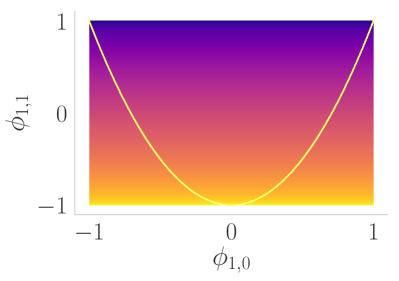
(a)

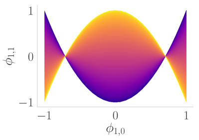
(b)

Figure 1: (a) Eigenfunction $\phi_{1,0}$ versus ${\phi}_{2,0}$ (curve) or ${\phi}_{0,1}$ (two dimensional manifold). (b) Eigenfunction $\phi_{1,0}$ versus ${\phi}_{1,1}$. All three manifolds are colored by the parameterization $h$.

Consider a continuous two dimensional strip with width $W$, height $H$, and aspect ratio $W/H\geq 1$, parametrized by coordinates $w\in[0,W],h\in[0,H]$. The eigenvalues and eigenfunctions of the Laplace-Beltrami operator $\Delta$ with von Neumann boundary conditions [Str07] are $\lambda_{k_{1},k_{2}}=\left(\tfrac{k_{1}\pi}{W}\right)^{2}+\left(\tfrac{k_{2}\pi}{H}\right)^{2}$, respectively $\phi_{k_{1},k_{2}}(w,h)=\cos\left(\frac{k_{1}\pi w}{W}\right)\cos\left(\frac{k_{2}\pi h}{H}\right)$. Eigenfunctions $\phi_{1,0}$, $\phi_{0,1}$ are in bijection with the $w,h$ coordinates (and give a full rank embedding), while the mapping by $\phi_{1,0},\phi_{2,0}$ provides no extra information regarding the second dimension $h$ in the underlying manifold (and is rank 1). Theoretically, one can choose as coordinates eigenfunctions indexed by $(k_{1},0),(0,k_{2})$, but, in practice, $k_{1}$, and $k_{2}$ are usually unknown, as the eigenvalues are index by their rank $0=\lambda_{0}<\lambda_{1}\leq\lambda_{2}\leq\cdots$. For a two dimensional strip, it is known [Str07] that $\lambda_{1,0}$ always corresponds to $\lambda_{1}$ and $\lambda_{0,1}$ corresponds to $\lambda_{(\lceil W/H\rceil)}$. Therefore, when $W/H>2$, the mapping of the strip to ${\mathbb{R}}^{2}$ by $\phi_{1},\phi_{2}$ is low rank, while the mapping by $\phi_{1},\phi_{\lceil W/H\rceil}$ is full rank. Note that other mappings of rank 2 exist, e.g., $\phi_{1},\phi_{\lceil W/H\rceil+2}$ ($k_{1}=k_{2}=1$ in Figure 1b). These embeddings reflect progressively higher frequencies, as the corresponding eigenvalues grow larger.

Prior work

[GZKR08] is the first work to give the IES problem a rigurous analysis. Their paper focuses on rectangles, and the failure illustrated in Figure 1a is defined as obtaining a mapping $\mathbf{\bm{Y}}=\phi(\mathbf{\bm{X}})$ that is not affinely equivalent with the original data. They call this the Price of Normalization and explain it in terms of the variances along $w$ and $h$. [DTCK18] is the first to frame the failure in terms of the rank of $\phi_{S}=\{\phi_{k}:k\in S\subseteq[m]\}$, calling it the repeated eigendirection problem. They propose a heuristic, LLRCoordSearch, based on the observation that if $\phi_{k}$ is a repeated eigendirection of $\phi_{1},\cdots,\phi_{k-1}$, one can fit $\phi_{k}$ with local linear regreesion on predictors $\phi_{[k-1]}$ with low leave-one-out errors $r_{k}$.

Existence of solution

Before trying to find an algorithmic solution to the IES problem, we ask the question whether this is even possible, in the smooth manifold setting. Positive answers are given in [Por16], which proves that isometric embeddings by DM with finite $m$ are possible, and more recently in [Bat14], which proves that any closed, connected Riemannian manifold $\mathcal{M}$ can be smoothly embedded by its Laplacian eigenfunctions $\phi_{[m]}$ into ${\mathbb{R}}^{m}$ for some $m$, which depends only on the intrinsic dimension $d$ of $\mathcal{M}$, the volume of $\mathcal{M}$, and lower bounds for injectivity radius and Ricci curvature. The example in Figure 1a demonstrates that, typically, not all $m$ eigenfunctions are needed. I.e., there exists a set $S\subset[m]$, so that $\phi_{S}$ is also a smooth embedding. We follow [DTCK18] in calling such a set $S$ independent. It is not known how to find an independent $S$ analytically for a given $\mathcal{M}$, except in special cases such as the strip. In this paper, we propose a finite sample and algorithmic solution, and we support it with asymptotic theoretical analysis.

The IES Problem

We are given data $\mathbf{\bm{X}}$, and the output of an embedding algorithm (DM for simplicity) $\mathbf{\bm{Y}}=\phi(\mathbf{\bm{X}})=[\phi_{1},\cdots,\phi_{m}]\in{\mathbb{R}}^{n\times m}$. We assume that $\mathbf{\bm{X}}$ is sampled from a $d$-dimensional manifold $\mathcal{M}$, with known $d$, and that $m$ is sufficiently large so that $\phi(\mathcal{M})$ is a smooth embedding. Further, we assume that there is a set $S\subseteq[m]$, with $|S|=s\leq m$, so that $\phi_{S}$ is also a smooth embedding of $\mathcal{M}$. We propose to find such set $S$ so that the rank of $\phi_{S}$ is $d$ on $\mathcal{M}$ and $\phi_{S}$ varies as slowly as possible.

Challenges

(1) Numerically, and on a finite sample, distiguishing between a full rank mapping and a rank-defective one is imprecise. Therefore, we substitute for rank the volume of a unit parallelogram in $\mathcal{T}_{\phi(\mathbf{\bm{x}}_{i})}\phi(\mathcal{M})$. (2) Since $\phi$ is not an isometry, we must separate the local distortions introduced by $\phi$ from the estimated rank of $\phi$ at $\mathbf{\bm{x}}$. (3) Finding the optimal balance between the above desired properties. (4) In [Bat14] it is strongly suggested that $s$ the number of eigenfunctions needed may exceed the Whitney embedding dimension ($\leq 2d$) [Lee03], and that this number may depend on injectivity radius, aspect ratio, and so on. Section 5 shows an example of a flat 2-manifold, the strip with cavity, for which $s>2$. In this paper, we assume that $s$ and $m$ are given and focus on selecting $S$ with $|S|=s$ unless otherwise stated; for completeness, in Section 5 we present a heuristic to select $s$.

(Global) functional dependencies, knots and crossings

Before we proceed, we describe three different ways a mapping $\phi(\mathcal{M})$ can fail to be invertible. The first, (global) functional dependency is the case when $\operatorname{rank}\textbf{{D}}\phi<d$ on an open subset of $\mathcal{M}$, or on all of $\mathcal{M}$ (yellow curve in Figure 1a); this is the case most widely recognized in the literature (e.g., [GZKR08, DTCK18]). The knot is the case when $\operatorname{rank}\textbf{{D}}\phi<d$ at an isolated point (Figure 1b). Third, the crossing (Figure S8 in Supplement G) is the case when $\phi:\mathcal{M}\rightarrow\phi(\mathcal{M})$ is not invertible at $\mathbf{\bm{x}}$, but $\mathcal{M}$ can be covered with open sets $U$ such that the restriction $\phi:U\rightarrow\phi(U)$ has full rank $d$. Combinations of these three exemplary cases can occur. The criteria and approach we define are based on the (surrogate) rank of $\phi$, therefore they will not rule out all crossings. We leave the problem of crossings in manifold embeddings to future work, as we believe that it requires an entirely separate approach (based, e.g., or the injectivity radius or density in the co-tangent bundle rather than differential structure).

4 Criteria and algorithm

4.1 A geometric criterion

We start with the main idea in evaluating the quality of a subset $S$ of coordinate functions. At each data point $i$, we consider the orthogonal basis $\mathbf{\bm{U}}(i)\in\mathbb{R}^{m\times d}$ of the $d$ dimensional tangent subspace $\mathcal{T}_{\phi(\mathbf{\bm{x}}_{i})}\phi(\mathcal{M})$. The projection of the columns of $\mathbf{\bm{U}}(i)$ onto the subspace $\mathcal{T}_{\phi(\mathbf{\bm{x}}_{i})}\phi_{S}(\mathcal{M})$ is $\mathbf{\bm{U}}(i)[S,:]\equiv\mathbf{\bm{U}}_{S}(i)$. The following Lemma connects $\mathbf{\bm{U}}_{S}(i)$ and the co-metric $\mathbf{\bm{H}}_{S}(i)$ defined by $\phi_{S}$, with the full $\mathbf{\bm{H}}(i)$.

Lemma 1.

Let $\mathbf{\bm{H}}(i)=\mathbf{\bm{U}}(i)\mathbf{\bm{\Sigma}}(i)\mathbf{\bm{U}}(i)^{\top}$ be the co-metric defined by embedding $\phi$, $S\subseteq[m]$, $\mathbf{\bm{H}}_{S}(i)$ and $\mathbf{\bm{U}}_{S}(i)$ defined above. Then $\mathbf{\bm{H}}_{S}(i)=\mathbf{\bm{U}}_{S}(i)\mathbf{\bm{\Sigma}}(i)\mathbf{\bm{U}}_{S}(i)^{\top}=\mathbf{\bm{H}}(i)[S,S]$.

The proof is straightforward and left to the reader. Note that Lemma 1 is responsible for the efficiency of the search over sets $S$, given that the push-forward co-metric $\mathbf{\bm{H}}_{S}$ can be readily obtained as a submatrix of $\mathbf{\bm{H}}$. Denote by $\mathbf{\bm{u}}^{S}_{k}(i)$ the $k$-th column of $\mathbf{\bm{U}}_{S}(i)$. We further normalize each $\mathbf{\bm{u}}^{S}_{k}$ to length 1 and define the normalized projected volume $\operatorname{Vol}_{\mathrm{norm}}(S,i)=\frac{\sqrt{\det(\mathbf{\bm{U}}_{S}(i)^{\top}\mathbf{\bm{U}}_{S}(i))}}{\prod_{k=1}^{d}\|\mathbf{\bm{u}}^{S}_{k}(i)\|_{2}}$. Conceptually, $\operatorname{Vol}_{\mathrm{norm}}(S,i)$ is the volume spanned by a (non-orthonormal) “basis” of unit vectors in $\mathcal{T}_{\phi_{S}(\mathbf{\bm{x}}_{i})}\phi_{S}(\mathcal{M})$; $\operatorname{Vol}_{\mathrm{norm}}(S,i)=1$ when $\mathbf{\bm{U}}_{S}(i)$ is orthogonal, and it is 0 when $\operatorname{rank}\mathbf{\bm{H}}_{S}(i)<d$. In Figure 1a, the $\operatorname{Vol}_{\mathrm{norm}}(\{1,2\})$ with $\phi_{\{1,2\}}=\{{\phi}_{1,0},{\phi}_{2,0}\}$ is close to zero, since the projection of the two tangent vectors is parallel to the yellow curve; however $\operatorname{Vol}_{\mathrm{norm}}(\{1,\lceil w/h\rceil\},i)$ is almost 1, because the projections of the tangent vectors $\mathbf{\bm{U}}(i)$ will be (approximately) orthogonal. Hence, $\operatorname{Vol}_{\mathrm{norm}}(S,i)$ away from 0 indicates a non-singular $\phi_{S}$ at $i$, and we use the average $\log\operatorname{Vol}_{\mathrm{norm}}(S,i)$, which penalizes values near 0 highly, as the rank quality ${\mathfrak{R}}(S)$ of $S$.

Higher frequency $\phi_{S}$ maps with high ${\mathfrak{R}}(S)$ may exist, being either smooth, such as the embeddings of the strip mentioned previously, or containing knots involving only small fraction of points, such as $\phi_{\phi_{1,0},\phi_{1,1}}$ in Figure 1a. To choose the lowest frequency, slowest varying smooth map, a regularization term consisting of the eigenvalues $\lambda_{k}$, $k\in S$, of the graph Laplacian $\mathbf{\bm{L}}$ is added, obtaining the criterion

$${\mathfrak{L}}(S;\zeta)=\underbrace{\frac{1}{n}\sum_{i=1}^{n}\log\sqrt{\det\left({\mathbf{\bm{U}}}_{S}(i)^{\top}{\mathbf{\bm{U}}}_{S}(i)\right)}}_{{\mathfrak{R}}_{1}(S)=\frac{1}{n}\sum_{i=1}^{n}{\mathfrak{R}}_{1}(S;i)}-\underbrace{\frac{1}{n}\sum_{i=1}^{n}\sum_{k=1}^{d}\log\|{\mathbf{\bm{u}}}^{S}_{k}(i)\|_{2}}_{{\mathfrak{R}}_{2}(S)=\frac{1}{n}\sum_{i=1}^{n}{\mathfrak{R}}_{2}(S;i)}-\zeta\sum_{k\in S}\lambda_{k}$$ (2)

4.2 Search algorithm

Input : Data $\mathbf{\bm{X}}$, bandwith $\varepsilon$, intrinsic dimension $d$, embedding dimension $s$, regularizer $\zeta$

1 $\mathbf{\bm{Y}}\in\mathbb{R}^{n\times m},\mathbf{\bm{L}},\mathbf{\bm{\lambda}}\in\mathbb{R}^{m}\leftarrow$DiffMap$(\mathbf{\bm{X}},\varepsilon)$

2 $\mathbf{\bm{U}}(i),\cdots,\mathbf{\bm{U}}(n)\leftarrow$RMetric$(\mathbf{\bm{Y}},\mathbf{\bm{L}},d)$

3 for $S\in\{S^{\prime}\subseteq[m]:|S^{\prime}|=s,1\in S^{\prime}\}$ do

4       ${\mathfrak{R}}_{1}(S)\leftarrow 0;{\mathfrak{R}}_{2}(S)\leftarrow 0$

5       for $i=1,\cdots,n$ do

6             $\mathbf{\bm{U}}_{S}(i)\leftarrow\mathbf{\bm{U}}(i)[S,:]$

7             ${\mathfrak{R}}_{1}(S)\mathrel{+}=\frac{1}{2n}\cdot\log\det\left(\mathbf{\bm{U}}_{S}(i)^{\top}\mathbf{\bm{U}}_{S}(i)\right)$

8             ${\mathfrak{R}}_{2}(S)\mathrel{+}=\frac{1}{n}\cdot\sum_{k=1}^{d}\log\|u^{S}_{k}(i)\|_{2}$

9       end for

10      ${\mathfrak{L}}(S;\zeta)={\mathfrak{R}}_{1}(S)-{\mathfrak{R}}_{2}(S)-\zeta\sum_{k\in S}\lambda_{k}$

11 end for

12$S_{*}=\operatorname*{argmax}_{S}{\mathfrak{L}}(S;\zeta)$

Return : Independent eigencoordinates set $S_{*}$

Algorithm 2 IndEigenSearch

With this criterion, the IES problem turns into a subset selection problem parametrized by $\zeta$

$$S_{*}(\zeta)=\operatorname*{argmax}_{S\subseteq[m];|S|=s;1\in S}{\mathfrak{L}}(S;\zeta)$$ (3)

Note that we force the first coordinate $\phi_{1}$ to always be chosen, since this coordinate cannot be functionally dependent on previous ones, and, in the case of DM, it also has lowest frequency. Note also that ${\mathfrak{R}}_{1}$ and ${\mathfrak{R}}_{2}$ are both submodular set function (proof in Supplement C.1). For large $s$ and $d$, algorithms for optimizing over the difference of submodular functions can be used (e.g., see [IB12]). For the experiments in this paper, we have $m=20$ and $d,s=2\sim 4$, which enables us to use exhaustive search to handle (3). The exact search algorithm is summarized in Algorithm 2 IndEigenSearch. A greedy variant is also proposed and analyzed in Supplement D.

4.3 Regularization path and choosing $\zeta$

According to (2), the optimal subset $S_{*}$ depends on the parameter $\zeta$. The regularization path $\ell(\zeta)=\max_{S\subseteq[m];|S|=s;1\in S}{\mathfrak{L}}(S;\zeta)$ is the upper envelope of multiple lines (each correspond to a set $S$) with slopes $-\sum_{k\in S}\lambda_{k}$ and intercepts ${\mathfrak{R}}(S)$. The larger $\zeta$ is, the more the lower frequency subset penalty prevails, and for sufficiently large $\zeta$ the algorithm will output $[s]$. In the supervised learning framework, the regularization parameters are often chosen by cross validation. Here we propose a second criterion, that effectively limits how much ${\mathfrak{R}}(S)$ may be ignored, or alternatively, bounds $\zeta$ by a data dependent quantity. Define the leave-one-out regret of point $i$ as follows

$$\mathfrak{D}(S,i)=\mathfrak{R}(S_{*}^{i};[n]\backslash\{i\})-\mathfrak{R}(S;[n]\backslash\{i\})\text{ with }S_{*}^{i}=\mathrm{argmax}_{S\subseteq[m];|S|=s;1\in S}{\mathfrak{R}}(S;i)$$ (4)

In the above, we denote $\mathfrak{R}(S;T)=\frac{1}{|T|}\sum_{i\in T}{\mathfrak{R}}_{1}(S;i)-{\mathfrak{R}}_{2}(S;i)$ for some subset $T\subseteq[n]$. The quantity $\mathfrak{D}(S,i)$ in (4) measures the gain in ${\mathfrak{R}}$ if all the other points $[n]\backslash\{i\}$ choose the optimal subset $S_{*}^{i}$. If the regret $\mathfrak{D}(S,i)$ is larger than zero, it indicates that the alternative choice might be better compared to original choice $S$. Note that the mean value for all $i$, i.e., $\frac{1}{n}\sum_{i}\mathfrak{D}(S,i)$ depends also on the variability of the optimal choice of points $i$, $S_{*}^{i}$. Therefore, it might not favor an $S$, if $S$ is optimal for every $i\in[n]$. Instead, we propose to inspect the distribution of $\mathfrak{D}(S,i)$, and remove the sets $S$ for which $\alpha$’s percentile are larger than zero, e.g., $\alpha=75\%$, recursively from $\zeta=\infty$ in decreasing order. Namely, the chosen set is $S_{*}=S_{*}(\zeta^{\prime})$ with $\zeta^{\prime}=\max_{\zeta\geq 0}\textsc{Percentile}(\{\mathfrak{D}(S_{*}(\zeta),i)\}_{i=1}^{n},\alpha)\leq 0$. The optimal $\zeta_{*}$ value is simply chosen to be the midpoint of all the $\zeta$’s that outputs set $S_{*}$ i.e., $\zeta_{*}=\frac{1}{2}\left(\zeta^{\prime}+\zeta^{\prime\prime}\right)$, where $\zeta^{\prime\prime}=\min_{\zeta\geq 0}S_{*}(\zeta)=S_{*}(\zeta^{\prime})$. The procedure ReguParamSearch is summarized in Algorithm 3.

Input : Threshold parameter $\alpha$

1 for $\zeta=\zeta_{\mathrm{\max}}\to 0$ do

       $\triangleright$ $\zeta_{\mathrm{\max}}$ should be sufficiently large such that $S_{*}(\zeta_{\max})=[s]$

2       $S\leftarrow S_{*}(\zeta)$; $S_{*}\leftarrow$NULL; $\zeta^{\prime\prime}\leftarrow$ NULL

3       for $i\in[n]$ do

4             $\mathfrak{D}(S,i)\leftarrow{\mathfrak{R}}(S^{i}_{*};[n]\backslash\{i\})-{\mathfrak{R}}(S;[n]\backslash\{i\})$ from equation (4)

5            

6       end for

7      if $\textsc{Percentile}(\{\mathfrak{D}(S,i)\}_{i=1}^{n},\alpha)\leq 0$ and $S_{*}=$ NULL  then

8             Optimal set $S_{*}\leftarrow S$

             $\zeta^{\prime}\leftarrow\zeta$   $\triangleright$ First found a set that satisfies the criterion.

9            

10       else if $S_{*}\neq$ NULL and $S_{*}=S_{*}(\zeta)$ then

             $\zeta^{\prime\prime}\leftarrow\zeta$   $\triangleright$ Searching for $\zeta^{\prime\prime}$

11            

12       else if $S_{*}\neq$ NULL and $\zeta^{\prime\prime}\neq$ NULL and $S_{*}\neq S_{*}(\zeta)$ then

13             $\zeta_{*}\leftarrow\frac{1}{2}(\zeta^{\prime}+\zeta^{\prime\prime})$

             break    $\triangleright$ Leave the loop when found $\zeta^{\prime\prime}=\min_{\zeta\geq 0}S_{*}(\zeta^{\prime})=S_{*}(\zeta)$

14            

15       else

16            continue

17       end if

18      

19 end for

Return : Optimal set $S_{*}$, optimal regularization parameter $\zeta_{*}$

Algorithm 3 ReguParamSearch

5 A heuristic to determine whether $s$ is sufficiently large

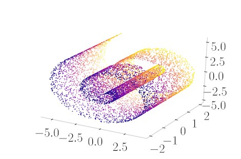
(a)

(b)

(c)

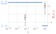
(d)

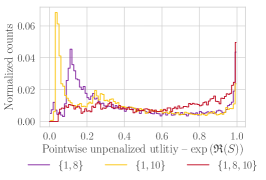
(e)

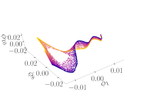
(f)

(g)

Figure 2: (a) Original data of $\mathcal{D}_{4}$, swiss roll with hole dataset. Embeddings with coordinate subset to be (b) $S=\{1,8\}$, (c) $S=\{1,10\}$, (f) $S=\{1,8,10\}$ and (g) $S=\{1,11\}$ on $\mathcal{D}_{4}$. (e) Histogram of point-wise normalized projected volume on $\mathcal{D}_{4}$ for top two ranking of subsets (purple and yellow) and the union of two sets (red) obtain from IndEigenSearch algorithm.

In this section, we propose a heuristic method to determine whether the given $s$ is large enough. Our method is based on the histogram of $\operatorname{Vol}_{\rm norm}(S,i)=\exp\left({\mathfrak{R}}(S,i)\right)$, the normalized projected volume of each point $i$. Recall that this volume is bounded between 0 and 1. Ideally, a perfect choice of cardinality $|S|$ will result in a concentration of mass in larger $\operatorname{Vol}_{\rm norm}$ region. The heuristic works as follow: at first we check the histogram of unpenalized $\operatorname{Vol}_{\rm norm}$ on the top few ranked subsets in terms of ${\mathfrak{L}}$. If spikes in the small $\operatorname{Vol}_{\rm norm}$ regions are witnessed in the histogram, taking the union of the subsets and inspecting the histogram of unpenalized $\operatorname{Vol}_{\rm norm}$ on the combined set again. If spikes in small $\operatorname{Vol}_{\rm norm}$ region diminished, one can conclude that a larger cardinality size $|S|$ is needed for such manifold.

We illustrate the idea on swiss roll with hole dataset in Figure 2a. Figure 2b is the optimal subset of coordinates $S_{*}=\{1,8\}$ selected by the proposed algorithm that best parameterize the underlying manifold. Figure 2d suggests one should eliminate $S_{0}=\{1,2\}$ because $\mathfrak{D}(S_{0},i)\geq 0$ for all the points by ReguParamSearch. However, as shown in Figure 2b, though it has low frequency and having rank $2$ for most of the places, set $\{1,8\}$ might not be suitable for data analysis for the very thin arms in left side of the embedding. Figure 2e is the histograms of the point-wise unpenalized $\operatorname{Vol}_{\rm norm}$ on different subsets. Purple and yellow curves correspond to the histogram of top two ranked subsets $S$ from IndEigenSearch. Both curves show a concentration of masses in small $\operatorname{Vol}_{\rm norm}$ region. The histogram of point-wise unpenalized $\operatorname{Vol}_{\rm norm}$ on $\{1,8,10\}$ (red curve), which is the union of the aforementioned two subsets, shows less concentration in the small $\operatorname{Vol}_{\rm norm}$ region and implies that $|S|=3$ might be a better choice for data analysis. Figure 2f shows the embedding with coordinate $S=\{1,8,10\}$, which represents a two dimensional strip embedded in three dimensional space. The thin arc in Figure 2b turns out to be a collapsed two dimensional manifold via projection, as shown in the upper right part of Figure 2f and left part of Figure 2c. Here we have to restate that the embedding in Figure 2b, although is a degenerated embedding, is still the best set one can choose for $s=2$ such that the embedding varies slowest and has rank $2$. However, choosing $s=3$ might be better for data analysis.

6 ${\mathfrak{R}}$ as Kullbach-Leibler divergence

In this section we analyze ${\mathfrak{R}}$ in its population version, and show that it is reminiscent of a Kullbach-Leibler divergence between unnormalized measures on $\phi_{S}(\mathcal{M})$. The population version of the regularization term takes the form of a well-known smoothness penalty on the embedding coordinates $\phi_{S}$.

Volume element and the Riemannian metric

Consider a Riemannian manifold $(\mathcal{M},g)$ mapped by a smooth embedding $\phi_{S}$ into $(\phi_{S}(\mathcal{M}),g_{*\phi_{S}})$, $\phi_{S}:\mathcal{M}\rightarrow{\mathbb{R}}^{s}$, where $g_{*\phi_{S}}$ is the push-forward metric defined in (1). A Riemannian metric $g$ induces a Riemannian measure on $\mathcal{M}$, with volume element $\sqrt{\det g}$. Denote now by $\mu_{\mathcal{M}}$, respectively $\mu_{\phi_{S}(\mathcal{M})}$ the Riemannian measures corresponding to the metrics induced on $\mathcal{M},\phi_{S}(\mathcal{M})$ by the ambient spaces ${\mathbb{R}}^{D},{\mathbb{R}}^{s}$; let $g$ be the former metric.

Lemma 2.

Let $S,\phi,\phi_{S},\mathbf{\bm{H}}_{S}(\mathbf{\bm{x}}),\mathbf{\bm{U}}_{S}(\mathbf{\bm{x}}),\mathbf{\bm{\Sigma}}(\mathbf{\bm{x}})$ be defined as in Section 4 and Lemma 1. For simplicity, we denote by $\mathbf{\bm{H}}_{S}(\mathbf{\bm{y}})\equiv\mathbf{\bm{H}}_{S}(\phi_{S}^{-1}(\mathbf{\bm{y}}))$, and similarly for $\mathbf{\bm{U}}_{S}(\mathbf{\bm{y}}),\mathbf{\bm{\Sigma}}(\mathbf{\bm{y}})$. Assume that $\phi_{S}$ is a smooth embedding. Then, for any measurable function $f:\mathcal{M}\rightarrow{\mathbb{R}}$,

$$\int_{\mathcal{M}}f(\mathbf{\bm{x}})d\mu_{\mathcal{M}}(\mathbf{\bm{x}})=\!\int_{\phi_{S}(\mathcal{M})}\!\!\!f(\phi_{S}^{-1}(\mathbf{\bm{y}}))j_{S}(y)d\mu_{\phi_{S}(\mathcal{M})}(\mathbf{\bm{y}}),$$ (5)

with

$$j_{S}(\mathbf{\bm{y}})\;=\;1/\operatorname{Vol}(\mathbf{\bm{U}}_{S}(\mathbf{\bm{y}})\mathbf{\bm{\Sigma}}_{S}^{1/2}(\mathbf{\bm{y}})).$$ (6)

Proof. Let $\mu^{*}_{\phi_{S}(\mathcal{M})}$ denote the Riemannian measure induced by $g_{*\phi_{S}}$. Since $(\mathcal{M},g)$ and $(\phi_{S}(\mathcal{M}),g_{*\phi_{S}})$ are isometric by definition, $\int_{\mathcal{M}}f(\mathbf{\bm{x}})d\mu_{\mathcal{M}}(\mathbf{\bm{x}})=\int_{\phi_{S}(\mathcal{M})}\!f(\phi_{S}^{-1}(\mathbf{\bm{y}}))d\mu^{*}_{\phi_{S}(\mathcal{M})}(\mathbf{\bm{y}})=\int_{\phi_{S}(\mathcal{M})}$$f(\phi_{S}^{-1}(\mathbf{\bm{y}}))$$\sqrt{\det g_{*\phi_{S}}(\mathbf{\bm{y}})}d\mu_{\phi_{S}(\mathcal{M})}(\mathbf{\bm{y}})$ follows from the change of variable formula. It remains to find the expression of $j_{S}(\mathbf{\bm{y}})=\sqrt{\det g_{*\phi_{S}}(\mathbf{\bm{y}})}$. The matrix $\mathbf{\bm{U}}_{S}(\mathbf{\bm{y}})$ (note that $\mathbf{\bm{U}}_{S}(\mathbf{\bm{y}})$ is not orthogonal) can be written as

$$\mathbf{\bm{U}}_{S}(\mathbf{\bm{y}})\;=\;\mathbf{\bm{V}}\mathbf{\bm{Q}}_{S}(\mathbf{\bm{y}})$$ (7)

where $\mathbf{\bm{V}}\in{\mathbb{R}}^{s\times d}$ is an orthogonal matrix and $\mathbf{\bm{Q}}_{S}(\mathbf{\bm{y}})\in{\mathbb{R}}^{d\times d}$ is upper triangular. Then,

$$\mathbf{\bm{H}}_{S}(\mathbf{\bm{y}})=\mathbf{\bm{U}}_{S}(\mathbf{\bm{y}})\mathbf{\bm{\Sigma}}(\mathbf{\bm{y}})\mathbf{\bm{U}}_{S}(y)^{\top}=\mathbf{\bm{V}}_{S}(y)\underbrace{(\mathbf{\bm{Q}}_{S}(\mathbf{\bm{y}})\mathbf{\bm{\Sigma}}(\mathbf{\bm{y}})\mathbf{\bm{Q}}_{S}(\mathbf{\bm{y}})^{\top})}_{\tilde{\mathbf{\bm{H}}}_{S}(\mathbf{\bm{y}})}\mathbf{\bm{V}}_{S}(\mathbf{\bm{y}})^{\top}.$$ (8)

In the above $\tilde{\mathbf{\bm{H}}}_{S}(y)$ is the co-metric expressed in the new coordinate system induced by $\mathbf{\bm{V}}_{S}(\mathbf{\bm{y}})$. Hence, in the same basis, $g_{*\phi_{S}}$ is expressed by

$$\tilde{\mathbf{\bm{G}}}_{S}(y)\,=\,\tilde{\mathbf{\bm{H}}}_{S}(y)^{-1}\,=\;(\mathbf{\bm{Q}}_{S}(\mathbf{\bm{y}})\mathbf{\bm{\Sigma}}(\mathbf{\bm{y}})\mathbf{\bm{Q}}_{S}(\mathbf{\bm{y}})^{\top})^{-1}.$$ (9)

The volume element, which is invariant to the chosen coordinate system, is

$$\det\left(\mathbf{\bm{Q}}_{S}(\mathbf{\bm{y}})\mathbf{\bm{\Sigma}}(\mathbf{\bm{y}})\mathbf{\bm{Q}}_{S}(\mathbf{\bm{y}})^{\top}\right)^{-1/2}\;=\;\prod_{k=1}^{d}\sigma_{k}(\mathbf{\bm{y}})^{-1/2}q_{S,kk}(\mathbf{\bm{y}})^{-1}.$$ (10)

From (7), it follows also that

$$\det\left(\mathbf{\bm{Q}}_{S}(\mathbf{\bm{y}})\mathbf{\bm{\Sigma}}(\mathbf{\bm{y}})\mathbf{\bm{Q}}_{S}(\mathbf{\bm{y}})^{\top}\right)^{-1/2}=1/\operatorname{Vol}\left(\mathbf{\bm{U}}_{S}(\mathbf{\bm{y}})\mathbf{\bm{\Sigma(\mathbf{\bm{y}})}}^{1/2}\right)$$ (11)

$\blacksquare$

Asymptotic limit of ${\mathfrak{R}}$

We now study the first term of our criterion in the limit of infinite sample size. We make the following assumptions.

Assumption 1.

The manifold $\mathcal{M}$ is compact of class $\mathcal{C}^{3}$, and there exists a set $S$, with $|S|=s$ so that $\phi_{S}$ is a smooth embedding of $\mathcal{M}$ in ${\mathbb{R}}^{s}$.

Assumption 2.

The data are sampled from a distribution on $\mathcal{M}$ continuous with respect to $\mu_{\mathcal{M}}$, whose density is denoted by $p$.

Assumption 3.

The estimate of $\mathbf{\bm{H}}_{S}$ in Algorithm 1 computed w.r.t. the embedding $\phi_{S}$ is consistent.

We know from [Bat14] that Assumption 1 is satisfied for the DM/LE embedding. The remaining assumptions are minimal requirements ensuring that limits of our quantities exist. Now consider the setting in Sections 3, in which we have a larger set of eigenfunctions, $\phi_{[m]}$ so that $[m]$ contains the set $S$ of Assumption 1. Denote by $\tilde{\jmath}_{S}(\mathbf{\bm{y}})=\prod_{k=1}^{d}\left(||u_{k}^{S}(\mathbf{\bm{y}})||\sigma_{k}(\mathbf{\bm{y}}))^{1/2}\right)^{-1}$ a new volume element.

Theorem 3 (Limit of ${\mathfrak{R}}$).

Under Assumptions 1–3,

$$\lim_{n\rightarrow\infty}\frac{1}{n}\sum_{i}\ln{\mathfrak{R}}(S,\mathbf{\bm{x}}_{i})={\mathfrak{R}}(S,\mathcal{M}),$$ (12)

and

$${\mathfrak{R}}(S,\mathcal{M})\,=\,-\int_{\phi_{S}(\mathcal{M})}\ln\frac{j_{S}(\mathbf{\bm{y}})}{\tilde{\jmath}_{S}(\mathbf{\bm{y}})}p(\phi_{S}^{-1}(\mathbf{\bm{y}}))j_{S}(\mathbf{\bm{y}})d\mu_{\phi_{S}(\mathcal{M})}(\mathbf{\bm{y}})\,\stackrel{{\scriptstyle\textit{def}}}{{=}}\,-D(pj_{S}\|p\tilde{\jmath}_{S})$$ (13)

Proof. Because $\phi_{S}$ is a smooth embedding, $j_{S}(\mathbf{\bm{y}})>0$ on $\phi_{S}(\mathcal{M})$, and because $\mathcal{M}$ is compact, $\min_{\phi_{S}(\mathcal{M})}j_{S}(\mathbf{\bm{y}})>0$. Similarly, noting that $\tilde{\jmath}_{S}(\mathbf{\bm{y}})\geq\prod_{k=1}^{d}\sigma_{k}^{-1/2}(\mathbf{\bm{y}})$, we conclude that $\tilde{\jmath}_{S}(\mathbf{\bm{y}})$ is also bounded away from 0 on $\mathcal{M}$. Therefore $\ln j_{S}(\mathbf{\bm{y}})$ and $\ln\tilde{\jmath}_{S}(\mathbf{\bm{y}})$ are bounded, and the integral in the r.h.s. of (13) exists and has a finite value. Now,

$$\frac{1}{n}\sum_{i}\ln{\mathfrak{R}}(S,\mathbf{\bm{x}}_{i})\,\rightarrow\,\int_{\mathcal{M}}\ln{\mathfrak{R}}(S,\mathbf{\bm{x}})p(\mathbf{\bm{x}})d\mu_{\mathcal{M}}(\mathbf{\bm{x}})\,=\,{\mathfrak{R}}(S,\mathcal{M}).$$ (14)

$$\int_{\mathcal{M}}\ln{\mathfrak{R}}(S,\mathbf{\bm{x}})p(\mathbf{\bm{x}})d\mu_{\mathcal{M}}(\mathbf{\bm{x}})$$

$$= \int_{\phi_{S}(\mathcal{M})}\ln{\mathfrak{R}}(\phi_{S}^{-1}(\mathbf{\bm{y}}))p(\phi_{S}^{-1}(\mathbf{\bm{y}}))j_{S}(\mathbf{\bm{y}})d\mu_{\phi_{S}(\mathcal{M})}(\mathbf{\bm{y}})$$

$$= \!\!\!\int_{\phi_{S}(\mathcal{M})}\!\!\left[\frac{1}{2}\ln\frac{\operatorname{Vol}\left(\mathbf{\bm{U}}^{\top}_{S}(\mathbf{\bm{y}})\mathbf{\bm{U}}_{S}(\mathbf{\bm{y}})\right)}{\tilde{\jmath}_{S}(\mathbf{\bm{y}})}-\frac{p(\phi_{S}^{-1}(\mathbf{\bm{y}})\prod_{k=1}^{d}\sigma_{k}^{1/2}(\mathbf{\bm{y}})}{p(\phi_{S}^{-1}(\mathbf{\bm{y}})\prod_{k=1}^{d}\sigma_{k}^{1/2}(\mathbf{\bm{y}})}\right]p(\phi_{S}^{-1}(\mathbf{\bm{y}}))j_{S}(\mathbf{\bm{y}})d\mu_{\phi_{S}(\mathcal{M})}(\mathbf{\bm{y}})$$

$$= \int_{\phi_{S}(\mathcal{M})}\ln\frac{j_{S}(\mathbf{\bm{y}})p(\phi_{S}^{-1}(\mathbf{\bm{y}})}{\tilde{\jmath}_{S}(\mathbf{\bm{y}})p(\phi_{S}^{-1}(\mathbf{\bm{y}})}p(\phi_{S}^{-1}(\mathbf{\bm{y}}))j_{S}(\mathbf{\bm{y}})d\mu_{\phi_{S}(\mathcal{M})}(\mathbf{\bm{y}})\;=\;-D(pj_{S}\|p\tilde{\jmath}_{S})$$ (16)

$\blacksquare$

Note that $D(\cdot\|\cdot)$ is a Kullbach-Leibler divergence, where the measures defined by $pj_{S},p\tilde{\jmath}_{S}$ normalize to different values; because $j_{S}\geq\tilde{\jmath}_{S}$ the divergence $D$ is always positive.

It is known that $\lambda_{k}$, the $k$-th eigenvalue of the Laplacian, converges under certain technical conditions [BN07] to an eigenvalue of the Laplace-Beltrami operator $\Delta_{\mathcal{M}}$ and that

$$\lambda_{k}(\Delta_{\mathcal{M}})=\langle\phi_{k},\Delta_{\mathcal{M}}\phi_{k}\rangle=\int_{\mathcal{M}}\|\operatorname{grad}\phi_{k}(\mathbf{\bm{x}})\|^{2}_{2}d\mu(\mathcal{M}).$$ (17)

Hence, a smaller value for the regularization term encourages the use of slow varying coordinate functions, as measured by the squared norm of their gradients, as in equation (17). Hence, under Assumptions 1, 2, 3, ${\mathfrak{L}}$ converges to

$${\mathfrak{L}}(S,\mathcal{M})\;=\;-D(pj_{S}\|p\tilde{\jmath}_{S})-\frac{\zeta}{\lambda_{1}(\mathcal{M})}\sum_{k\in S}\lambda_{k}(\mathcal{M}).$$ (18)

The rescaling of $\zeta$ in comparison with equation (2) aims to make $\zeta$ adimensional, whereas the eigenvalues scale with the volume of $\mathcal{M}$.

7 Experiments

	Original data $\mathbf{\bm{X}}$	Embedding ${\phi}_{S_{*}}$	Regularization path
$\mathcal{D}_{1}$
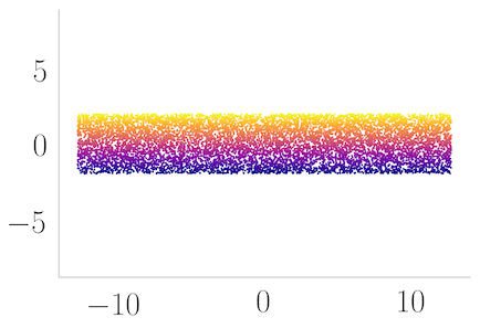
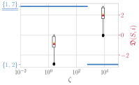
$\mathcal{D}_{7}$
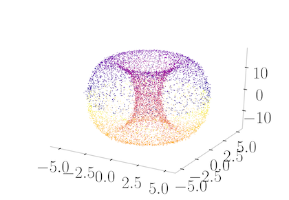
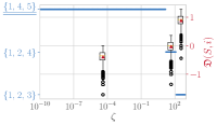
$\mathcal{D}_{13}$

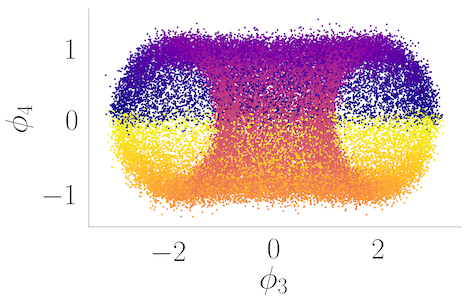
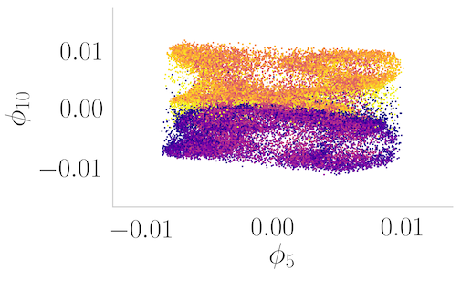
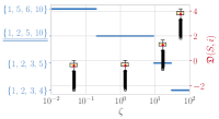
Figure 3: Experimental result for synthetic datasets. Rows correspond to different synthetic datasets (please refer to Table S2). Optimal subset $S_{*}$ is selected by IndEigenSearch.

We demonstrate the proposed algorithm on three synthetic datasets, one where the minimum embedding dimension $s$ equals $d$ ($\mathcal{D}_{1}$ long strip), and two ($\mathcal{D}_{7}$ high torus and $\mathcal{D}_{13}$ three torus) where $s>d$. The complete list of synthetic manifolds (transformations of 2 dimensional strips, 3 dimensional cubes, two and three tori, etc.) investigated can be found in Supplement G and Table S2. The examples have (i) aspect ratio of at least 4 (ii) points sampled non-uniformly from the underlying manifold $\mathcal{M}$, and (iii) Gaussian noise added. The sample size of the synthetic datasets is $n=10,000$ unless otherwise stated. Additionally, we analyze several real datasets from chemistry and astronomy. All embeddings are computed with the DM algorithm, which outputs $m=20$ eigenvectors. Hence, we examine 171 sets for $s=3$ and $969$ sets for $s=4$. No more than 2 to 5 of these sets appear on the regularization path. Detailed experimental results are in Table S3. In this section, we show the original dataset $\mathbf{\bm{X}}$, the embedding $\phi_{S_{*}}$, with $S_{*}$ selected by IndEigenSearch and $\zeta_{*}$ from ReguParamSearch, and the maximizer sets on the regularization path with box plots of $\mathfrak{D}(S,i)$ as discussed in Section 4. The $\alpha$ threshold for ReguParamSearch is set to $75\%$. All the experiments are replicated for more than 5 times, and the outputs are similar because of the large sample size $n$.

Synthetic manifolds The results of synthetic manifolds are in Figure 3. (i) Manifold with $s=d$. The first synthetic dataset we considered, $\mathcal{D}_{1}$, is a two dimensional strip with aspect ratio $W/H=2\pi$. Left panel of the top row shows the scatter plot of such dataset. From the theoretical analysis in Section 3, the coordinate set that corresponds to slowest varying unique eigendirection is $S=\{1,\lceil W/H\rceil\}=\{1,7\}$. Middle panel, with $S_{*}=\{1,7\}$ selected by IndEigenSearch with $\zeta$ chosen by ReguParamSearch, confirms this. The right panel shows the box plot of $\{\mathfrak{D}(S,i)\}_{i=1}^{n}$. According to the proposed procedure, we eliminate $S_{0}=\{1,2\}$ since $\mathfrak{D}(S_{0},i)\geq 0$ for almost all the points. (ii) Manifold with $s>d$. The second data $\mathcal{D}_{7}$ is displayed in the left panel of the second row. Due to the mechanism we used to generate the data, the resultant torus is non-uniformly distributed along the z axis. Middle panel is the embedding of the optimal coordinate set $S_{*}=\{1,4,5\}$ selected by IndEigenSearch. Note that the middle region (in red) is indeed a two dimensional narrow tube when zoomed in. The right panel indicates that both $\{1,2,3\}$ and $\{1,2,4\}$ (median is around zero) should be removed. The optimal regularization parameter is $\zeta_{*}\approx 7$. The result of the third dataset $\mathcal{D}_{13}$, three torus, is in the third row of the figure. We displayed only projections of the penultimate and the last coordinate of original data $\mathbf{\bm{X}}$ and embedding $\phi_{S_{*}}$ (which is $\{5,10\}$) colored by $\alpha_{1}$ of (S7) in the left and middle panel to conserve space. A full combinations of coordinates can be found in Figure S5. The right panel implies one should eliminate the set $\{1,2,3,4\}$ and $\{1,2,3,5\}$ since both of them have more than $75\%$ of the points such that $\mathfrak{D}(S,i)\geq 0$. The first remaining subset is $\{1,2,5,10\}$, which yields an optimal regularization parameter $\zeta_{*}\approx 5$.

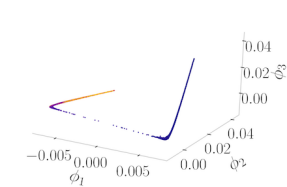
(a)

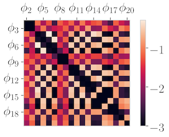
(b)

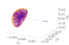
(c)

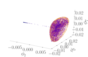
(d)

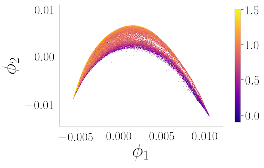
(e)

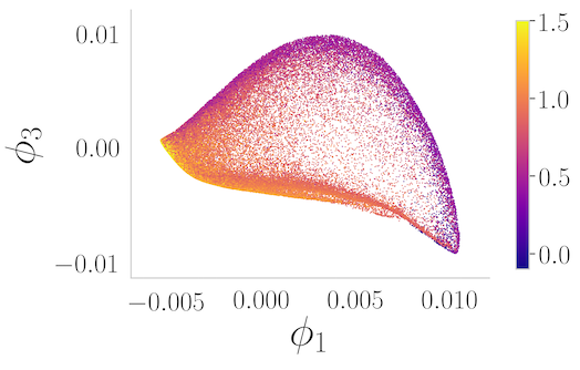
(f)

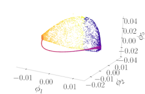
(g)

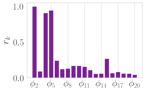
(h)

Figure 4: First row: Choloromethane dataset; second row: SDSS dataset in (e), (f) and (g), (h) show the example when LLR failed. (c) and (d) are embeddings with top two ranked subsets $S_{1}$ and $S_{2}$, colored by the distances between C and two different Cl-, respectively. (e) and (f) are embeddings of $\mathbf{\bm{\phi}}_{\{1,2\}}$ (suboptimal set) and $\mathbf{\bm{\phi}}_{\{1,3\}}$ (maximizer of ${\mathfrak{L}}$), respectively (values shown in caption).

Molecular dynamics dataset [FTP16]

In SN2 reaction molecular dynamics of chloromethane [FTP16] dataset, two chloride atoms substitute with each other in different configurations/points $\mathbf{\bm{x}}_{i}$ as described in the following chemical equation CH3Cl + Cl^- ¡-¿ CH3Cl + Cl^-. The dataset exhibits some kind of clustering structure with a sparse connection between two clusters which represents the time when the substitution happened. The dataset has size $n\approx 30,000$ and ambient dimension $D=40$, with the intrinsic dimension estimate be $\hat{d}=2$ The embedding with coordinate set $S=[3]$ is shown in Figure 4a. The first three eigenvectors parameterize the same directions, which yields a one dimensional manifold in the figure. Top view ($S=[2]$) of the figure is a u-shaped structure similar to the yellow curve in Figure 1a. The heat map of ${\mathfrak{L}}(\{1,i,j\})$ for different combinations of coordinates in Figure 4b confirms that ${\mathfrak{L}}$ for $S=[3]$ is low and that $\phi_{1}$, $\phi_{2}$ and $\phi_{3}$ give a low rank mapping. The heat map also shows high ${\mathfrak{L}}$ values for $S_{1}=\{1,4,6\}$ or $S_{2}=\{1,5,7\}$, which correspond to the top two ranked subsets. The embeddings with $S_{1},S_{2}$ are in Figures 4c and 4d, respectively. In this case, we obtain two optimal $S$ sets due to the data symmetry.

Galaxy spectra from the Sloan Digital Sky survey (SDSS)

[AAMA⁺09], preprocessed as in [MMVZ16]. We display a sample of $n=50,000$ points from the first $0.3$ million points which correspond to closer galaxies. Figures 4e and 4f show that the first two coordinates are almost dependent; the embedding with $S_{*}=\{1,3\}$ is selected by IndEigenSearch with $d=2$. Both plots are colored by the blue spectrum magnitude, which is correlated to the number of young stars in the galaxy, showing that this galaxy property varies smoothly and non-linearly with $\phi_{1},\phi_{3}$, but is not smooth w.r.t. $\phi_{1},\phi_{2}$.

Comparison with [DTCK18]

The LLRCoordSearch method outputs similar candidate coordinates as our proposed algorithm most of the time (see Table S3). However, the results differ for high torus as in Figure 4. Figure 4h is the leave one out (LOO) error $r_{k}$ versus coordinates. The coordinates chosen by LLRCoordSearch was $S=\{1,2,5\}$, as in Figure 4g. The embedding is clearly shown to be suboptimal, for it failed to capture the cavity within the torus. This is because the algorithm searches in a sequential fashion; the noise eigenvector $\phi_{2}$ in this example appears before the signal eigenvectors e.g., $\phi_{4}$ and $\phi_{5}$.

Additional experiments with real data

are shown in Table 1. Not surprisingly, for most real data sets we examined, the independent coordinates are not the first $s$. They also show that the algorithm scales well and is robust to the noise present in real data.

Table 1: Results for other real datasets. Columns from left to right are sample size $n$, ambient dimension of data $D$, average degree of neighbor graph $\mathrm{deg}_{\mathrm{avg}}$, $(s,d)$ and runtime for IES, and the chosen set $S^{*}$, respectively. Last three datasets are from [CTS⁺17].

	$n$	$D$	$\mathrm{deg}_{\mathrm{avg}}$	$(s,d)$	$t$ (sec)	$S^{*}$
SDSS (full)	298,511	3750	144.91	(2, 2)	106.05	(1, 3)
Aspirin	211,762	244	101.03	(4, 3)	85.11	(1, 2, 3, 7)
Ethanol	555,092	102	107.27	(3, 2)	233.16	(1, 2, 4)
Malondialdehyde	993,237	96	106.51	(3, 2)	459.53	(1, 2, 3)

The asymptotic runtime of LLRCoordSearch has quadratic dependency on $n$, while for our algorithm is linear in $n$. Details of runtime analysis are Supplement E. LLRCoordSearch was too slow to be tested on the four larger datasets (see also Figure S1).

8 Conclusion

Algorithms that use eigenvectors, such as DM, are among the most promising and well studied in ML. It is known since [GZKR08] that when the aspect ratio of a low dimensional manifold exceeds a threshold, the choice of eigenvectors becomes non-trivial, and that this threshold can be as low as 2. Our experimental results confirm the need to augment ML algorithms with IES methods in order to successfully apply ML to real world problems. Surprisingly, the IES problem has received little attention in the ML literature, to the extent that the difficulty and complexity of the problem have not been recognized. Our paper advances the state of the art by (i) introducing for the first time a differential geometric definition of the problem, (ii) highlighting geometric factors such as injectivity radius that, in addition to aspect ratio, influence the number of eigenfunctions needed for a smooth embedding, (iii) constructing selection criteria based on intrinsic manifold quantities, (iv) which have analyzable asymptotic limits, (v) can be computed efficiently, and (vi) are also robust to the noise present in real scientific data. The library of hard synthetic examples we constructed will be made available along with the python software implementation of our algorithms.

Disclaimer

The views expressed herein do not necessarily represent the views of the U.S. Department of Energy or the United States Government.

Supplement to
Selecting the independent coordinates of manifolds with large aspect ratios

Appendix A Notational table

Table S1: Notational table

Matrix operation
$\mathbf{\bm{M}}$	Matrix
$\mathbf{\bm{m}}_{i}$	Vector represents the $i$-th row of $\mathbf{\bm{M}}$
$\mathbf{\bm{m}}_{:,j}^{T}$	Vector represents the $j$-th column of $\mathbf{\bm{M}}$
$m_{ij}$	Scalar represents $ij$-th element of $\mathbf{\bm{M}}$
$[\mathbf{\bm{M}}]_{ij}$	Scalar, alternative notation for $m_{ij}$
$\mathbf{\bm{M}}[\alpha,\beta]$	Submatrix of $\mathbf{\bm{M}}$ of index sets $\alpha,\beta$
$\mathbf{\bm{v}}$	Column vector
$v_{i}$	Scalar represents $i$-th element of vector $\mathbf{\bm{v}}$
$[\mathbf{\bm{v}}]_{i}$	Scalar, alternative notation for $v_{i}$
Scalars
$n$	Number of samples
$D$	Ambient dimension
$m$	Dimension of diffusion embedding
$s$	(Minimum) embedding dimension
$d$	Intrinsic dimension
Vectors & Matrices
$\mathbf{\bm{X}}$	Data matrix
$\mathbf{\bm{x}}_{i}$	Point $i$ in ambient space
$\mathbf{\bm{Y}}$	Diffusion coordinates
$\mathbf{\bm{y}}_{i}$	Point $i$ in diffusion coordinates
$\phi_{i}$	The $i$-th diffusion coordinate of all points
$\mathbf{\bm{K}}$	Kernel (similarity) matrix
$\mathbf{\bm{L}}$	Graph Laplacian
$\mathbf{\bm{H}}(i)$	Dual metric at point $i$
$\mathbf{\bm{I}}_{k}$	Identity matrix in $k$ dimension space
$\mathbf{\bm{1}}_{n}$	All one vector $\in\mathbb{R}^{n}$
$\mathbf{\bm{1}}_{S}$	$[\mathbf{\bm{1}}_{S}]_{i}=1$ if $i\in S$ 0 otherwise
Miscellaneous
$G(V,E)$	Graph with vertex set $V$ and edge set $E$
$\mathcal{M}$	Data manifold
$\phi(\cdot)$	Embedding mapping
${\mathfrak{L}}(S;\zeta)$	Utilities
${\mathfrak{R}}$	Unpenalized utilities
$[s]$	Set $\{1,\cdots,s\}$
$D(\cdot\|\cdot)$	KL divergence
D	Jacobian
$\mathfrak{D}(S,i)$	Leave-one-out regret of point $i$

Appendix B Pseudocodes

Input : Data matrix $\mathbf{\bm{X}}\in{\mathbb{R}}^{n\times D}$, bandwidth $\varepsilon$, embedding dimension $m$

1 Compute similarity matrix $\mathbf{\bm{K}}$ with $K_{ij}=\begin{cases}\exp\left[-\frac{||\mathbf{\bm{x}}_{i}-\mathbf{\bm{x}}_{j}||^{2}}{\varepsilon^{2}}\right]&\text{ if }\|x-y\|\leq 3\varepsilon\\ 0&\text{ otherwise }\end{cases}$

2 $\mathbf{\bm{L}}\leftarrow\text{{\sc Laplacian}}(\mathbf{\bm{K}})\in{\mathbb{R}}^{n\times n}$ (Algorithm 5)

3 Compute eigenvectors of $\mathbf{\bm{L}}$ for smallest $m+1$ eigenvalues $[\mathbf{\bm{\phi}}_{0}\,\mathbf{\bm{\phi}}_{1}\,\ldots\mathbf{\bm{\phi}}_{m}]\in{\mathbb{R}}^{n\times(m+1)}$

Return : $\mathbf{\bm{\Phi}}=[\mathbf{\bm{\phi}}_{1}\,\ldots\mathbf{\bm{\phi}}_{m}]\in{\mathbb{R}}^{n\times m}$ The embedding coordinates of $\mathbf{\bm{x}}_{i}$ are $(\Phi_{i1},\ldots,\Phi_{im})\in{\mathbb{R}}^{m}$

Algorithm 4 DiffMap

Input : Symmetric similarity matrix $\mathbf{\bm{K}}$

Calculate the degree of node $i$, $[\mathbf{\bm{w}}]_{i}=\sum_{j=1}^{n}K_{ij}$ $\triangleright$ Set $\mathbf{\bm{W}}=\operatorname{diag}(\mathbf{\bm{w}})$

1 $\tilde{\mathbf{\bm{L}}}=\mathbf{\bm{W}}^{-1}\mathbf{\bm{K}}\mathbf{\bm{W}}^{-1}$

$[\tilde{\mathbf{\bm{w}}}]_{i}\leftarrow\sum_{j=1}^{n}\tilde{L}_{ij}$ $\triangleright$ Set $\tilde{\mathbf{\bm{W}}}=\operatorname{diag}(\tilde{\mathbf{\bm{w}}})$

2 $\mathbf{\bm{L}}=\mathbf{\bm{I}}_{n}-\tilde{\mathbf{\bm{W}}}^{-1}\tilde{\mathbf{\bm{L}}}$

Return : Renormalized graph Laplacian $\mathbf{\bm{L}}$

Algorithm 5 Laplacian

Input : Embedding $\mathbf{\bm{Y}}=[\phi_{1},\cdots,\phi_{m}]\in\mathbb{R}^{n\times m}$

1 Set the leave-one-out validation error $\mathbf{\bm{r}}=[1,\cdots,1]\in\mathbb{R}^{m}$

2 for $s=2\to m$ do

3       Bandwidth of LLR: $h\leftarrow\frac{1}{3}\cdot\textsc{Median}(\textsc{PairwiseDist}(\phi_{[s-1]}))$

4       $\hat{\phi}_{s}\leftarrow$ LocalLinearRegression$(\phi_{s},\phi_{[s-1]},h)$

5       $r_{s}=\sqrt{\frac{\|\hat{\phi}_{s}-\phi_{s}\|^{2}}{\|\phi_{s}\|^{2}}}$

6 end for

7$S_{*}\leftarrow\textsc{ArgSort}(\mathbf{\bm{r}})$

$\triangleright$ Sort in descending order.

Return : Sorted independent coordinates $S_{*}$

Algorithm 6 LLRCoordSearch

Appendix C Extra theorems

C.1 Submodularity of the objective functions

Theorem S1.

For a rank $d$ tangent space matrix $\mathbf{\bm{U}}\in\mathbb{R}^{m\times d}$, if any submatrix $\mathbf{\bm{U}}_{S}$, with index set $S\subseteq[m]$ and $|S|=s\geq d$, is rank $d$, we have ${\mathfrak{R}}_{1}$ be a submodular set function.

Proof. W.L.O.G, set $n=1$, with slightly abuse of notation, let $\mathbf{\bm{U}}=\mathbf{\bm{U}}_{T\cup\{i\}}\in\mathbb{R}^{(|T|+1)\times d}$. The matrix can be written in the following form

$$\mathbf{\bm{U}}=\begin{bmatrix}\mathbf{\bm{T}}\\ \mathbf{\bm{a}}\end{bmatrix}=\begin{bmatrix}\mathbf{\bm{S}}\\ \mathbf{\bm{V}}\\ \mathbf{\bm{a}}\end{bmatrix}\in\mathbb{R}^{(|T|+1)\times d}$$

With $\mathbf{\bm{U}}_{S}=\mathbf{\bm{S}}$, $\mathbf{\bm{U}}_{T}=\mathbf{\bm{T}}$ and $U_{\{i\}}=\mathbf{\bm{a}}$ for set $S\subseteq T\subseteq[m]$ and $i\in[m]\backslash T$. Here $\mathbf{\bm{a}}\in\mathbb{R}^{1\times d}$. By the definition of ${\mathfrak{R}}_{1}$ in (2), one has (ignoring the constants)

$$\begin{gathered}{\mathfrak{R}}_{1}(S)=\log\det(\mathbf{\bm{S}}^{\top}\mathbf{\bm{S}})\\ {\mathfrak{R}}_{1}(T)=\log\det\left(\mathbf{\bm{T}}^{\top}\mathbf{\bm{T}}\right)\\ {\mathfrak{R}}_{1}(S\cap\{i\})=\log\det\left(\begin{bmatrix}\mathbf{\bm{S}}\\ \mathbf{\bm{a}}\end{bmatrix}^{\top}\begin{bmatrix}\mathbf{\bm{S}}\\ \mathbf{\bm{a}}\end{bmatrix}\right)\\ {\mathfrak{R}}_{1}(T\cap\{i\})=\log\det(\mathbf{\bm{U}}^{\top}\mathbf{\bm{U}})\end{gathered}$$

Denote $\partial_{i}f(S)=f(S\cup\{i\})-f(S)$ for some function $f$, we have

$$\begin{gathered}\partial_{i}{\mathfrak{R}}_{1}(S)=\log\det(\mathbf{\bm{S}}^{\top}\mathbf{\bm{S}}+\mathbf{\bm{a}}^{\top}\mathbf{\bm{a}})-\log\det(\mathbf{\bm{S}}^{\top}\mathbf{\bm{S}})\\ \partial_{i}{\mathfrak{R}}_{1}(T)=\log\det(\mathbf{\bm{T}}^{\top}\mathbf{\bm{T}}+\mathbf{\bm{a}}^{\top}\mathbf{\bm{a}})-\log\det(\mathbf{\bm{T}}^{\top}\mathbf{\bm{T}})\end{gathered}$$

The full rank of any submatrices guarantees the positive definiteness of $\mathbf{\bm{S}}^{\top}\mathbf{\bm{S}},\mathbf{\bm{T}}^{\top}\mathbf{\bm{T}}$, by matrix determinant lemma [Har98], we have

$$\det(\mathbf{\bm{S}}^{\top}\mathbf{\bm{S}}+\mathbf{\bm{a}}^{\top}\mathbf{\bm{a}})=\det(\mathbf{\bm{S}}^{\top}\mathbf{\bm{S}})\left(1+\mathbf{\bm{a}}(\mathbf{\bm{S}}^{\top}\mathbf{\bm{S}})^{-1}\mathbf{\bm{a}}^{\top}\right)$$

Therefore

$$\partial_{i}{\mathfrak{R}}_{1}(S)=1+\mathbf{\bm{a}}(\mathbf{\bm{S}}^{\top}\mathbf{\bm{S}})^{-1}\mathbf{\bm{a}}^{\top}$$

Similar equation holds for set $T$. Therefore,

$$\partial_{i}{\mathfrak{R}}_{1}(S)-\partial_{i}{\mathfrak{R}}_{1}(T)=\log\frac{1+\mathbf{\bm{a}}(\mathbf{\bm{S}}^{\top}\mathbf{\bm{S}})^{-1}\mathbf{\bm{a}}^{\top}}{1+\mathbf{\bm{a}}(\mathbf{\bm{T}}^{\top}\mathbf{\bm{T}})^{-1}\mathbf{\bm{a}}^{\top}}$$

Because $\mathbf{\bm{T}}^{\top}\mathbf{\bm{T}}\succeq\mathbf{\bm{S}}^{\top}\mathbf{\bm{S}}$, we have $(\mathbf{\bm{S}}^{\top}\mathbf{\bm{S}})^{-1}\succeq(\mathbf{\bm{T}}^{\top}\mathbf{\bm{T}})^{-1}$ [HHJ90], which implies $\partial_{i}{\mathfrak{R}}_{1}(S)-\partial_{i}{\mathfrak{R}}_{1}(T)\geq 0$ for all $S\subseteq T\subseteq[m]$ and $i\in[m]\backslash T$. This completes the proof. $\blacksquare$

Theorem S2.

${\mathfrak{R}}_{2}$ is a submodular set function.

Proof. W.L.O.G, set $n,d=1$. With slightly abuse of notation, let $\mathbf{\bm{u}}\leftarrow\mathbf{\bm{u}}_{1}(i)$ and $\mathbf{\bm{u}}_{S}\leftarrow\mathbf{\bm{u}}^{S}_{1}(i)$. For any set $S\subseteq T\subseteq[m]$ and $i\in[m]\backslash T$, we have

$$\begin{gathered}\begin{split}\partial_{i}{\mathfrak{R}}_{2}(S)&={\mathfrak{R}}_{2}\left(S\cap\{i\}\right)-{\mathfrak{R}}_{2}(S)=\log\frac{\sum_{k\in S}u_{k}^{2}+u_{i}^{2}}{\sum_{k\in S}u_{k}^{2}}=\log\frac{\Sigma_{S}+u_{i}^{2}}{\Sigma_{S}}\end{split}\\ \begin{split}\partial_{i}{\mathfrak{R}}_{2}(T)&={\mathfrak{R}}_{2}\left(T\cap\{i\}\right)-{\mathfrak{R}}_{2}(T)=\log\frac{\sum_{k\in T}u_{k}^{2}+u_{i}^{2}}{\sum_{k\in T}u_{k}^{2}}=\log\frac{\Sigma_{S}+\Sigma_{T\backslash S}+u_{i}^{2}}{\Sigma_{S}+\Sigma_{T\backslash S}}\end{split}\end{gathered}$$

Where $\Sigma_{S}=\sum_{k\in S}u_{k}^{2}$. By definition, we have $\Sigma_{S},\Sigma_{T\backslash S},u_{i}^{2}\geq 0$. Therefore,

$$\begin{split}&\partial_{i}{\mathfrak{R}}_{2}(S)-\partial_{i}{\mathfrak{R}}_{2}(T)=\log\frac{\left(\Sigma_{S}+u_{i}^{2}\right)\cdot\left(\Sigma_{S}+\Sigma_{T\backslash S}\right)}{\Sigma_{S}\cdot\left(\Sigma_{S}+\Sigma_{T\backslash S}+u_{i}^{2}\right)}\\ &=\log\underbrace{\left[\frac{\Sigma_{S}^{2}+\Sigma_{S}\left(\Sigma_{T\backslash S}+u^{2}_{i}\right)+u_{i}^{2}\Sigma_{T\backslash S}}{\Sigma_{S}^{2}+\Sigma_{S}\left(\Sigma_{T\backslash S}+u^{2}_{i}\right)}\right]}_{\geq 1}\geq 0\end{split}$$

Which completes the proof. $\blacksquare$

Appendix D Greedy search

Input : Orthogonal basis $\{\mathbf{\bm{U}}(i)\}_{i=1}^{n}$, eigenvalues $\mathbf{\bm{\lambda}}$, intrinsic dimension $d$, regularization parameter $\zeta$

1 Solve $S_{*}\leftarrow\operatorname*{argmax}_{S\subseteq[m];|S|=d;1\in S}{\mathfrak{L}}(S;\zeta)$.

2 for $s=d+1\to m$ do

3       $k_{*}=\operatorname*{argmax}_{k\in[m]\backslash S_{*}}{\mathfrak{L}}(S_{*}\cup\{k\};\zeta)$

       $S_{*}\leftarrow S_{*}\cup\{k_{*}\}$ $\triangleright$ Record order

4      

5 end for

Return : Independent coordinates $S_{*}$

Algorithm 7 GreedyIndEigenSearch

Inspired by the greedy version of submodular maximization [NWF78], a greedy heuristic has been proposed, as in Algorithm 7. The algorithm starts from an observation that the optimal value of the $S^{\prime}=\operatorname*{argmax}_{S;d\leq|S|<s}{\mathfrak{L}}(S;\zeta)$ will often time be a subset of the optimal $S_{*}$ of (3). Since the appropriate cardinality of the set $S$ is unknown, we can simply scan from $|S|=d$ to $m$. The order of the returned elements indicates the significance of the corresponding coordinate.

Appendix E Computational complexity analysis

E.1 The proposed algorithms

For computation complexity analysis, we assume the embedding has already been obtained. Therefore, the computational complexity for building neighbor graph and solving the eigen-problem of graph Laplacian can be omitted. This is also the case for LLRCoordSearch.

Co-metrics and orthogonal basis

According to [PM13], time complexity for computing $\mathbf{\bm{H}}(i)\in\mathbb{R}^{m\times m}~{}\forall~{}i\in[n]$ is $\mathcal{O}(nm^{2}\delta)$, with $\delta$ be the average degree of the neighbor graph $G(V,E)$. In manifold learning, the graph will be sparse therefore $\delta\ll n$. Time complexity for obtaining principal space $\mathbf{\bm{U}}(i)$ of point $i$ via SVD will be $\mathcal{O}(m^{3})$. Total time complexity will be $\mathcal{O}(nm^{2}\delta+nm^{3})$.

Exact search

Evaluating the objective function ${\mathfrak{L}}$ for each point $i$ takes $\mathcal{O}(sd^{2})$ in computing $\mathbf{\bm{U}}_{S}(i)^{\top}\mathbf{\bm{U}}_{S}(i)$, $\mathcal{O}(d^{3})$ in evaluating the determinant of a $d\times d$ matrix. Normalization (${\mathfrak{R}}_{2}$ term) takes $\mathcal{O}(ds)$. Exhaustive search over all the subset with cardinality $s$ takes $\mathcal{O}\left(\binom{m}{s}\right)$. The total computational complexity will therefore be $\mathcal{O}(nm^{s}(d^{3}+d^{2}s)+nm^{2}\delta+nm^{3})=\mathcal{O}(nm^{s+3}+nm^{2}\delta)$.

Greedy algorithm

First step of greedy algorithm includes solving $\operatorname*{argmax}_{S\subseteq[m];|S|=d}{\mathfrak{L}}(S,d)$, which takes $\mathcal{O}(nm^{d}d^{3})=\mathcal{O}(nm^{d+3})$. Starting from $s=d+1\to m$, each step includes exhaustively search over $m-s$ candidates, with the time complexity of evaluating ${\mathfrak{L}}$ be $n(d^{3}+d^{2}s)$. Putting things together, one has the second part of the greedy algorithm be

$$\sum_{s=d}^{m}n(m-s)(d^{3}+d^{2}s)=\mathcal{O}(nm^{5})$$ (S1)

The total computational complexity will therefore be $\mathcal{O}(n(m^{d+3}+m^{5}+m^{2}\delta))$.

E.2 Time complexity of [DTCK18] & discussion

The Algorithm LLRCoordSearch is summarized in Algorithm 6. For searching over fixed coordinate $s$, the algorithm first build a kernel for local linear regression by constructing a neighbor graph, which takes $\mathcal{O}(n\log(n)s)$ using approximate nearest neighbor search. The $s$ dependency come from the dimension of the feature. For each point $i$, a ordinary least square (OLS) problem is solved, which results in $\mathcal{O}(n^{2}s^{2}+ns^{3})$ time complexity.

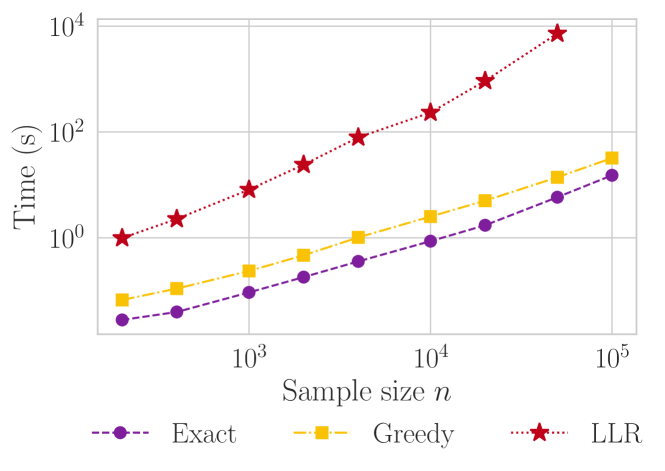
Figure S1: Runtimes of different IES algorithms on two dimensional long strip. Purple, yellow and red curves correspond to IndEigenSearch, GreedyIndEigenSearch and LLRCoordSearch algorithm, respectively.

Searching from $s=2\to m$ will make the total time complexity be

$$\sum_{s=2}^{m}n^{2}s^{2}+ns^{3}+ns\log n=\mathcal{O}(n^{2}m^{3}+nm^{4})$$ (S2)

For a sparse graph, the overheads of the IndEigenSearch and GreedyIndEigenSearch algorithms come from the enumeration of the subset $S$. Because of the linear dependency on the sample size $n$, the algorithm is tractable for small $s$ and $d$. However, LLRCoordSearch  has a quadratic dependency on sample size $n$, which is more computationally intensive for large sample size. For large $s$ and $d$, one can use the techniques in difference between submodular function optimization (e.g. [IB12]) as ${\mathfrak{R}}_{1}$, ${\mathfrak{R}}_{2}$ are both submodular set function from Theorems S1 and S2. An empirical runtime plot for different algorithms can be found in Figure S1. The runtime was evaluated on two dimensional long strip with $s=d=2$ and was performed on a single desktop computer running Linux with 32GB RAM and a 8-Core 4.20GHz Intel® Core™ i7-7700K CPU.

Appendix F A discussion on UMAP

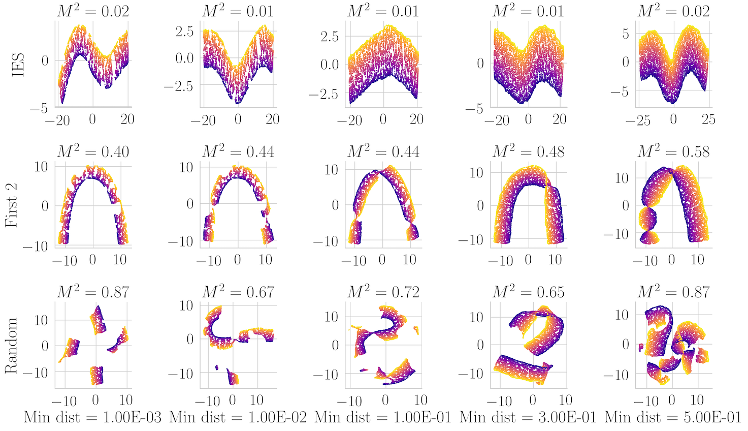
(a)

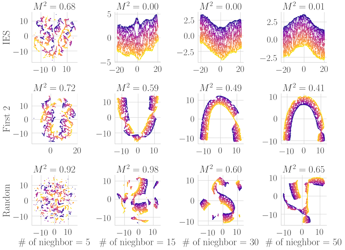
(b)

Figure S2: UMAP embeddings of 2D long stripe with different initializations and choices of hyper-parameters. Rows from top to bottom correspond to UMAP embedding initialized with DM which coordinates chosen by IndEigenSearch, naïve DM and random initialization, respectively. Columns represent different choices of (a) points separation and (b) number of neighbors.

UMAP [MHM18] is a commonly used data visualization alternative of t-SNE. The authors proposed to use the spectral embedding of the graph Laplacian as an initialization to the algorithm for faster convergence (compared to random initialization). In this section, we showed empirically that, (1) given reasonable computing resources, the IES problem also appears in the UMAP embedding and (2) by initializing with spectral embedding with carefully selected coordinate set chosen by IndEigenSearch, one can obtain a faster convergence and a globally interpretable embedding. Figure S2 is the UMAP embedding of 2D long stripe dataset $\mathcal{D}_{1}$ with different choices of hyper-parameters (points separation in S2a and number of neighbors in S2b), with total number of epochs be $500$. The first row of both plots are the embedding initialized with IndEigenSearch, the second row corresponds to those initialized with naïve DM. The embeddings in the third row are initialized randomly. As shown in the results, algorithmic/random artifacts can be easily seen in the embeddings with Naïve DM or random initialization (2nd and 3rd rows). More precisely, unwanted patterns which reduce the interpretability of the embeddings, e.g., the “knots” in the second row or disconnected components in the second/third rows, are generated. The sum of square procrustes error $M^{2}$ between ground truth dataset and the embedding shown on each subplots also confirm our statement. Note that it is possible to unroll the algorithmic artifact with more epochs in the sampling steps of UMAP. (3 to 5 times more iterations are needed in this example.) However, due to the efficiency of performing IndEigenSearch, it is beneficial to initialize with the embedding selected by IndEigenSearch.

Appendix G Additional experiments & details of the used datasets

In this paper, a total of 13 different synthetic manifolds are considered. Table S2 summarized the synthetic manifolds constructed and its abbreviations (from $\mathcal{D}_{1}$ to $\mathcal{D}_{13}$). Embedding results for the synthetic manifolds are in Figures S3, S4 and S5. The ranking of the first few candidate sets $S$ from IndEigenSearch, GreedyIndEigenSearchand LLRCoordSearch can be found in Table S3. The table shows the optimal subsets return by three different algorithms are often time the same, with exception for $\mathcal{D}_{7}$ high torus as discussed in Section 7.

Table S2: Abbreviations for different synthetic manifolds in this paper. The abbreviation with asterisk represents such dataset is discussed in main manuscript.

Manifold with $s=d$
$\mathcal{D}_{1}^{*}$	Two dimensional strip (aspect ratio $2\pi$)
$\mathcal{D}_{2}$	2D strip with cavity (aspect ratio $2\pi$)
$\mathcal{D}_{3}$	Swiss roll
$\mathcal{D}_{4}$	Swiss roll with cavity
$\mathcal{D}_{5}$	Gaussian manifold
$\mathcal{D}_{6}$	Three dimensional cube
Manifold with $s>d$
$\mathcal{D}_{7}^{*}$	High torus
$\mathcal{D}_{8}$	Wide torus
$\mathcal{D}_{9}$	z-asymmetrized high torus
$\mathcal{D}_{10}$	x-asymmetrized high torus
$\mathcal{D}_{11}$	z-asymmetrized wide torus
$\mathcal{D}_{12}$	x-asymmetrized wide torus
$\mathcal{D}_{13}^{*}$	Three-torus

Table S3: Results returned from different algorithms on different synthetic datasets.

	Exact search					Greedy rank	LLR rank
	1	2	3	4	5
$\mathcal{D}_{1}$	[1, 7]	[1, 8]	[1, 9]	[1, 10]	[1, 12]	[1, 7, 6, 4, 3, 2, 5]	[1, 7, 14, 16, 11, 18, 6]
$\mathcal{D}_{2}$	[1, 4]	[1, 8]	[1, 9]	[1, 10]	[1, 12]	[1, 4, 8, 6, 5, 3, 2]	[1, 4, 8, 5, 17, 11, 14]
$\mathcal{D}_{3}$	[1, 9]	[1, 10]	[1, 11]	[1, 13]	[1, 18]	[1, 9, 5, 2, 3, 4, 6]	[1, 9, 19, 16, 12, 10, 4]
$\mathcal{D}_{4}$	[1, 8]	[1, 10]	[1, 11]	[1, 14]	[1, 15]	[1, 8, 3, 2, 4, 10, 5]	[1, 8, 11, 10, 19, 16, 4]
$\mathcal{D}_{5}$	[1, 6]	[1, 8]	[1, 10]	[1, 11]	[1, 13]	[1, 6, 2, 8, 3, 10, 4]	[1, 6, 19, 8, 18, 14, 12]
$\mathcal{D}_{6}$	[1, 2, 8]	[1, 2, 11]	[1, 4, 8]	[1, 2, 17]	[1, 2, 13]	[1, 2, 8, 3, 4, 6, 5]	[1, 2, 8, 10, 3, 13, 6]
$\mathcal{D}_{7}$	[1, 4, 5]	[1, 4, 8]	[1, 5, 7]	[1, 7, 12]	[1, 7, 8]	[1, 5, 4, 3, 6, 2, 8]	[1, 2, 5, 4, 15, 6, 10]
$\mathcal{D}_{8}$	[1, 2, 7]	[1, 4, 7]	[1, 3, 7]	[1, 2, 9]	[1, 5, 7]	[1, 7, 2, 4, 3, 13, 5]	[1, 2, 7, 13, 12, 15, 14]
$\mathcal{D}_{9}$	[1, 3, 4]	[1, 3, 7]	[1, 4, 6]	[1, 3, 10]	[1, 7, 9]	[1, 3, 4, 2, 9, 7, 6]	[1, 3, 4, 2, 19, 8, 7]
$\mathcal{D}_{10}$	[1, 2, 4]	[1, 3, 4]	[1, 4, 5]	[1, 6, 9]	[1, 6, 14]	[1, 4, 2, 3, 5, 6, 8]	[1, 4, 2, 3, 8, 5, 6]
$\mathcal{D}_{11}$	[1, 2, 5]	[1, 4, 8]	[1, 4, 5]	[1, 8, 9]	[1, 2, 8]	[1, 5, 2, 4, 8, 3, 9]	[1, 2, 5, 8, 10, 9, 11]
$\mathcal{D}_{12}$	[1, 2, 5]	[1, 4, 5]	[1, 2, 7]	[1, 3, 5]	[1, 2, 8]	[1, 5, 2, 3, 4, 6, 8]	[1, 5, 2, 6, 10, 9, 4]
$\mathcal{D}_{13}$	[1, 2, 5, 10]	[1, 3, 5, 10]	[1, 4, 5, 10]	[1, 5, 6, 10]	[1, 2, 8, 10]	[1, 5, 10, 2, 4, 3, 6]	[1, 2, 10, 5, 14, 15, 16]

G.1 Additional experiments on synthetic manifolds with $s=d$

Below summarized the details of generating the datasets.

1. $\mathcal{D}_{1}^{*}$: points from this dataset are sampled uniformly from $\mathbf{\bm{x}}_{i}\sim\textsc{Unif}([-2,2]\times[-4\pi,4\pi])$.

2. $\mathcal{D}_{2}$: points are first sampled uniformly from $[-2,2]\times[-4\pi,4\pi]$. Points $i$ are removed if $|X_{i1}|<4\pi/3$ and $|X_{i2}|<2/3$.

3. $\mathcal{D}_{3}$: first sampling points $\mathbf{\bm{X}}_{\mathrm{true}}=[\mathbf{\bm{x}}_{0},\mathbf{\bm{y}}_{0}]$ uniformly from a two dimensional strip. The data $\mathbf{\bm{X}}$ can be obtained by the following non-linear transformation.

   $$\mathbf{\bm{X}}=\left[\frac{\mathbf{\bm{x}}_{0}\mathbin{\vbox{\hbox{{$\circ$}}}}\cos\mathbf{\bm{x}}_{0}}{2},\mathbf{\bm{y}}_{0},\frac{\mathbf{\bm{x}}_{0}\mathbin{\vbox{\hbox{{$\circ$}}}}\sin\mathbf{\bm{x}}_{0}}{2}\right]$$ (S3)

   With $\mathbin{\vbox{\hbox{{$\circ$}}}}$ denotes Hadamard (element-wise) product.

4. $\mathcal{D}_{4}$: sampling points $\mathbf{\bm{X}}_{\mathrm{true}}=[\mathbf{\bm{x}}_{0},\mathbf{\bm{y}}_{0}]$ uniformly from 2D strip with cavity then applying the transformation (S3) to get $\mathbf{\bm{X}}$.

5. $\mathcal{D}_{5}$: sampling points $\mathbf{\bm{X}}_{\mathrm{true}}$ uniformly from ellipse $\left\{(x,y)\in\mathbb{R}^{2}:\left(\frac{x}{6}\right)^{2}+\left(\frac{y}{2}\right)^{2}=1\right\}$. The data is obtained by

   $$\mathbf{\bm{X}}=\left[\mathbf{\bm{X}}_{\mathrm{true}},\mathbf{\bm{z}}\right]$$

   With $z_{i}=\exp\left(-\left(\left(\frac{X_{i1}}{3}\right)^{2}+X_{i2}^{2}\right)/2\right)$

6. $\mathcal{D}_{6}$: points are sampled uniformly from $[-1,1]\times[-2,2]\times[-4,4]$.

The experimental results are in Figure S3 ($\mathcal{D}_{4}$ in Figure 2).

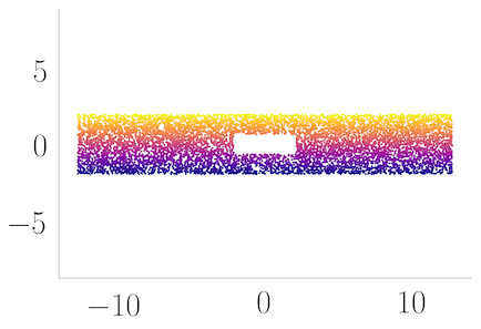
(a)

(b)

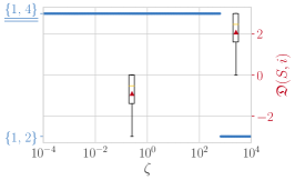
(c)

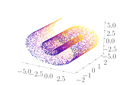
(d)

(e)

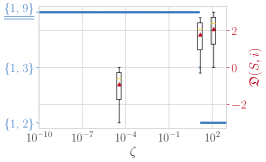
(f)

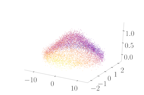
(g)

(h)

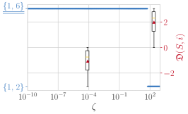
(i)

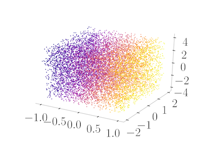
(j)

(k)

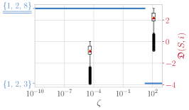
(l)

Figure S3: Synthetic manifolds with minimum embedding dimension $s$ equals intrinsic dimension $d$. Rows from top to bottom represent two dimensional strip with cavity (aspect ratio $W/H=2\pi$), swiss roll, gaussian manifold and three dimensional cube dataset, respectively. Columns from left to right are the original data $\mathbf{\bm{X}}$, embedding ${\phi}_{S_{*}}$ with optimal coordinate sets $S_{*}$ chosen by IndEigenSearch and the regularization path, respectively.

G.2 Additional experiments on synthetic manifolds with $s>d$

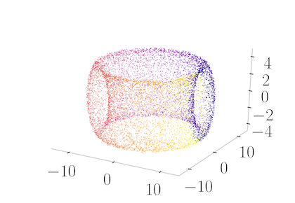
(a)

(b)

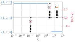
(c)

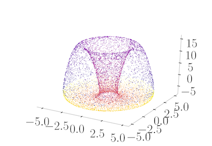
(d)

(e)

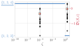
(f)

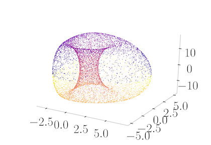
(g)

(h)

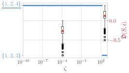
(i)

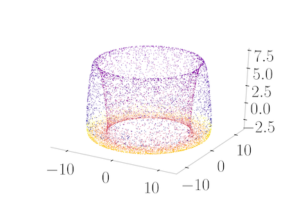
(j)

(k)

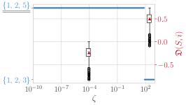
(l)

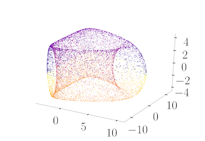
(m)

(n)

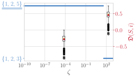
(o)

Figure S4: Synthetic manifolds with minimum embedding dimension $s$ greater than intrinsic dimension $d$. Rows from top to bottom represent wide torus, z-asymmetrized high torus, x-asymmetrized high torus, z-asymmetrized wide torus and x-asymmetrized wide torus, respectively. Columns from left to right are the original data $\mathbf{\bm{X}}$, embedding ${\phi}_{S_{*}}$ with optimal coordinate sets $S_{*}$ chosen by IndEigenSearch and the regularization path, respectively.

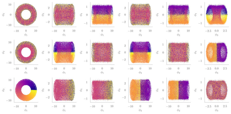
(a)

(b)

Figure S5: Experiment on three-torus dataset. (a) Original data $\mathbf{\bm{X}}$ of three torus. (b) Embedding ${\phi}_{S_{*}}$ with optimal coordinate sets $S_{*}$ chosen by IndEigenSearch. Rows for both (a) and (b) from top to bottom are embedding colored by the parameterization $(\alpha_{1},\alpha_{2},\alpha_{3})$ in (S7), respectively.

G.2.1 Tori and asymmetrized tori

A torus can be parametrized by

$$\begin{split}x&=(a+b\cos\alpha)\cos\beta\\ y&=(a+b\cos\alpha)\sin\beta\\ z&=h\sin(\beta)\end{split}$$ (S4)

1. $\mathcal{D}_{7}^{*}$: sampling $\mathbf{\bm{\alpha}},\mathbf{\bm{\beta}}$ uniformly from $[0,2\pi)$ and generating the torus with $(a,b,h)=(3,2,8)$ from (S4).

2. $\mathcal{D}_{8}$: generating the torus with $(a,b,h)=(10,2,2)$.

3. $\mathcal{D}_{9}$: generating a high torus with $(a,b,h)=(3,2,8)$ and applying the following transformation

   $$z\leftarrow(z-\min(z))^{\gamma}/\varsigma\\$$ (S5)

   with $(\gamma,\varsigma)=(3,1500)$

4. $\mathcal{D}_{10}$: generating a high torus with $(a,b,h)=(3,2,8)$ and applying the following transformation

   $$x\leftarrow(x-\min(x))^{\kappa}/\eta\\$$ (S6)

   with $(\kappa,\eta)=(2,10)$

5. $\mathcal{D}_{11}$: generating a wide torus with $(a,b,h)=(10,2,2)$ and applying transformation (S5) with $(\gamma,\varsigma)=(3,50)$.

6. $\mathcal{D}_{12}$: generating a wide torus with $(a,b,h)=(10,2,2)$ and applying transformation (S6) with$(\kappa,\eta)=(3,1000)$.

The experimental results are in Figure S4.

G.2.2 Three-torus

Figure S6: $M^{2}$ and $\hat{d}$ vs. ranking of $\mathcal{D}_{13}$

The parameterization of the three torus is

$$\begin{split}x_{1}&=a_{1}\sin\alpha_{1}\\ x_{2}&=(a_{2}+a_{1}\cos\alpha_{1})\sin\alpha_{2}\\ x_{3}&=(a_{3}+(a_{2}+a_{1}\cos\alpha_{1})\cos\alpha_{2})\sin\alpha_{3}\\ x_{4}&=(a_{3}+(a_{2}+a_{1}\cos\alpha_{1})\cos\alpha_{2})\cos\alpha_{3}\end{split}$$ (S7)

To generate $\mathcal{D}_{13}$, we sample $\mathbf{\bm{\alpha}}_{k}$ uniformly from $[0,2\pi)$ for $k\in[3]$ and apply the transformation (S7) with $(a_{1},a_{2},a_{3})=(8,2,1)$. The sample size for this dataset is $n=50,000$. The experimental result of three-torus can be found in Figure S5.

(a)

(b)

(c)

(d)

(e)

(f)

(g)

(h)

(i)

(j)

(k)

(l)

Figure S7: Verification of the correctness of the chosen sets in synthetic manifolds.

G.3 Verification of the chosen subsets on synthetic manifolds

Unlike 2D strip, the close form solution of the optimal set is oftentimes unknown in general. In this section, we verify the correctness of the chosen subset by reporting the full procrustes distance (disparity score) $M^{2}$ [Dry16], which is defined to be the normalized sum of square of the point-wise difference between the procrustes transformed ground truth data $\mathbf{\bm{X}}_{\mathrm{true}}\in{\mathbb{R}}^{n\times k}$ and the test data $\mathbf{\bm{X}}_{\mathrm{test}}\in{\mathbb{R}}^{n\times k}$. Namely,

$$\begin{split}M^{2}(\mathbf{\bm{X}}_{\mathrm{true}},\mathbf{\bm{X}}_{\mathrm{test}})&=\min_{\beta,\mathbf{\bm{\gamma}},\mathbf{\bm{\Gamma}}}\|\mathbf{\bm{X}}_{\mathrm{true}}-\beta\mathbf{\bm{X}}_{\mathrm{test}}\mathbf{\bm{\Gamma}}-\mathbf{\bm{1}}_{n}\mathbf{\bm{\gamma}}^{\top}\|_{F}^{2}\\ \text{ s.t. }&\beta>0,\mathbf{\bm{\gamma}}\in\mathbb{R}^{k},\Gamma\in SO(k)\end{split}$$ (S8)

Figure S8: Embedding that has crossing.

Here $\beta$ is a scale parameter, $\mathbf{\bm{\gamma}}$ is the centering parameter and $\mathbf{\bm{\Gamma}}$ is a $k\times k$ rotation matrix. We further require $\|\mathbf{\bm{X}}_{\mathrm{true}}\|_{F}=1$ so that the disparity score will be between 0 and 1. Intuitively, one can expect the optimal choice of eigencoordinates $S_{*}$ will yield a small disparity score $M^{2}(\mathbf{\bm{X}}_{\mathrm{true}},\phi_{S_{*}})$, with score increases as the coordinate set $S$ contains duplicate parameterizations or $\phi_{S}$ contains knots, crossings, etc. (e.g., Figure S8). Note that the score can only be calculated when the ground truth data $\mathbf{\bm{X}}_{\mathrm{true}}$ is available. For dataset without obtainable ground truth, one cannot proposed to report the disparity score of $\phi_{S}$ and the original data $\mathbf{\bm{X}}$ as the proxy of $\mathbf{\bm{X}}_{\mathrm{true}}$, for $\mathbf{\bm{X}}$ might not be a affine transformation of $\mathbf{\bm{X}}_{\mathrm{true}}$, e.g., Swiss roll. Besides, small $M^{2}$ given $\phi_{S}$ does not imply $S$ is optimal, which will be clear in the discussion of Figure 2g. Besides disparity scores, we will also report the estimated dimension $\hat{d}$. One can expect the estimated dimension for the optimal set $\dim(\phi_{S_{*}})$ will be close to the intrinsic dimension $d$, while the estimated dimension for sets containing duplicate parameterizations will be smaller than the intrinsic dimension. One cannot propose to use it as a criterion to choose the optimal set, for the suboptimal sets can also have estimated dimensions closed to the intrinsic dimension, e.g., Figure 4g. Throughout the experiment, the dimension estimation method by [LB05] is used for its ability to estimate dimension among all candidate subsets fairly fast. Blue and red curves in Figure S7 and S6 show the disparity scores and estimated dimensions versus ranking of coordinate subsets for different synthetic manifolds, respectively. As expected, we have an increasing in $M^{2}$ and decreasing in $\hat{d}$ with respect to ranking. We first highlight that the set that produces the lowest disparity score is not necessarily optimal, although $S_{*}$ does yield a small disparity. This can be shown in the example of $\mathcal{D}_{4}$ swiss roll with hole dataset. Figure 2g is the embedding ${\phi}_{S_{3}}$ of $\mathcal{D}_{4}$, with $S_{3}$ is ranked third subset in terms of ${\mathfrak{L}}(S;\zeta)$, that minimizes the disparity score $M^{2}$ in $\mathcal{D}_{4}$ as shown in Figure S7d. This is because the embedding of the subset $S_{3}=\{1,11\}$ has larger area on the left, compared to Figure Figure 2b. This balances out the high disparity caused by the flipped region between two knots in the embedding ${\phi}_{S_{3}}$ when matched with $\mathbf{\bm{X}}_{\mathrm{true}}$. Since all the ranked first subset has low disparity compared to other subsets, we have higher confidence saying that the ranked 1st subset is indeed the optimal choice for the synthetic manifolds.

References

- [AAMA+09] Kevork N Abazajian, Jennifer K Adelman-McCarthy, Marcel A Agüeros, Sahar S Allam, Carlos Allende Prieto, Deokkeun An, Kurt SJ Anderson, Scott F Anderson, James Annis, Neta A Bahcall, et al. The seventh data release of the sloan digital sky survey. The Astrophysical Journal Supplement Series, 182(2):543, 2009.
- [Bat14] Jonathan Bates. The embedding dimension of laplacian eigenfunction maps. Applied and Computational Harmonic Analysis, 37(3):516–530, 2014.
- [BN07] Mikhail Belkin and Partha Niyogi. Convergence of laplacian eigenmaps. In B. Schölkopf, J. C. Platt, and T. Hoffman, editors, Advances in Neural Information Processing Systems 19, pages 129–136. MIT Press, 2007.
- [CL06] R. R. Coifman and S. Lafon. Diffusion maps. Applied and Computational Harmonic Analysis, 30(1):5–30, 2006.
- [CTS+17] Stefan Chmiela, Alexandre Tkatchenko, Huziel E Sauceda, Igor Poltavsky, Kristof T Schütt, and Klaus-Robert Müller. Machine learning of accurate energy-conserving molecular force fields. Science advances, 3(5):e1603015, 2017.
- [Dry16] I. L. (Ian L.) Dryden. Statistical shape analysis : with applications in R. Wiley series in probability and statistics. Wiley, Chichester, West Sussex, England, 2nd ed. edition, 2016.
- [DS13] Sanjoy Dasgupta and Kaushik Sinha. Randomized partition trees for exact nearest neighbor search. In Conference on Learning Theory, pages 317–337, 2013.
- [DTCK18] Carmeline J Dsilva, Ronen Talmon, Ronald R Coifman, and Ioannis G Kevrekidis. Parsimonious representation of nonlinear dynamical systems through manifold learning: A chemotaxis case study. Applied and Computational Harmonic Analysis, 44(3):759–773, 2018.
- [FTP16] Kelly L. Fleming, Pratyush Tiwary, and Jim Pfaendtner. New approach for investigating reaction dynamics and rates with ab initio calculations. Jornal of Physical Chemistry A, 120(2):299–305, 2016.
- [GZKR08] Yair Goldberg, Alon Zakai, Dan Kushnir, and Ya’acov Ritov. Manifold learning: The price of normalization. Journal of Machine Learning Research, 9(Aug):1909–1939, 2008.
- [Har98] David A Harville. Matrix algebra from a statistician’s perspective, 1998.
- [HAvL05] Matthias Hein, Jean-Yves Audibert, and Ulrike von Luxburg. From graphs to manifolds - weak and strong pointwise consistency of graph laplacians. In Learning Theory, 18th Annual Conference on Learning Theory, COLT 2005, Bertinoro, Italy, June 27-30, 2005, Proceedings, pages 470–485, 2005.
- [HAvL07] Matthias Hein, Jean-Yves Audibert, and Ulrike von Luxburg. Graph laplacians and their convergence on random neighborhood graphs. Journal of Machine Learning Research, 8:1325–1368, 2007.
- [HHJ90] Roger A Horn, Roger A Horn, and Charles R Johnson. Matrix analysis. Cambridge university press, 1990.
- [IB12] Rishabh Iyer and Jeff Bilmes. Algorithms for approximate minimization of the difference between submodular functions, with applications. In Proceedings of the Twenty-Eighth Conference on Uncertainty in Artificial Intelligence, UAI’12, pages 407–417, Arlington, Virginia, United States, 2012. AUAI Press.
- [LB05] Elizaveta Levina and Peter J Bickel. Maximum likelihood estimation of intrinsic dimension. In Advances in neural information processing systems, pages 777–784, 2005.
- [Lee03] John M. Lee. Introduction to smooth manifolds, 2003.
- [MHM18] Leland McInnes, John Healy, and James Melville. Umap: Uniform manifold approximation and projection for dimension reduction. arXiv preprint arXiv:1802.03426, 2018.
- [MMVZ16] James McQueen, Marina Meilă, Jacob VanderPlas, and Zhongyue Zhang. Megaman: Scalable manifold learning in python. Journal of Machine Learning Research, 17(148):1–5, 2016.
- [NLCK06] Boaz Nadler, Stephane Lafon, Ronald Coifman, and Ioannis Kevrekidis. Diffusion maps, spectral clustering and eigenfunctions of Fokker-Planck operators. In Y. Weiss, B. Schölkopf, and J. Platt, editors, Advances in Neural Information Processing Systems 18, pages 955–962, Cambridge, MA, 2006. MIT Press.
- [NWF78] George L Nemhauser, Laurence A Wolsey, and Marshall L Fisher. An analysis of approximations for maximizing submodular set functions—i. Mathematical programming, 14(1):265–294, 1978.
- [PM13] D. Perraul-Joncas and M. Meila. Non-linear dimensionality reduction: Riemannian metric estimation and the problem of geometric discovery. ArXiv e-prints, May 2013.
- [Por16] Jacobus W Portegies. Embeddings of riemannian manifolds with heat kernels and eigenfunctions. Communications on Pure and Applied Mathematics, 69(3):478–518, 2016.
- [Str07] Walter A Strauss. Partial differential equations: An introduction. Wiley, 2007.
- [THJ10] Daniel Ting, Ling Huang, and Michael I. Jordan. An analysis of the convergence of graph laplacians. In Proceedings of the 27th International Conference on Machine Learning (ICML-10), pages 1079–1086, 2010.