A hp-adaptive discontinuous Galerkin solver for elliptic equations in numerical relativity

Abstract

A considerable amount of attention has been given to discontinuous Galerkin methods for hyperbolic problems in numerical relativity, showing potential advantages of the methods in dealing with hydrodynamical shocks and other discontinuities. This paper investigates discontinuous Galerkin methods for the solution of elliptic problems in numerical relativity. We present a novel hp-adaptive numerical scheme for curvilinear and non-conforming meshes. It uses a multigrid preconditioner with a Chebyshev or Schwarz smoother to create a very scalable discontinuous Galerkin code on generic domains. The code employs compactification to move the outer boundary near spatial infinity. We explore the properties of the code on some test problems, including one mimicking Neutron stars with phase transitions. We also apply it to construct initial data for two or three black holes.

I Introduction

Discontinuous Galerkin (DG) methods Reed and Hill (1973); Hesthaven and Warburton (2008); Cockburn (2001); Cockburn and Shu (1998); Cockburn (1998); Cockburn et al. (2000) have matured into standard numerical methods to simulate a wide variety of partial differential equations. In the context of numerical relativity Baumgarte and Shapiro (2010), discontinuous Galerkin methods have shown advantages for relativistic hyperbolic problems over traditional discretization methods such as finite difference, finite volume and spectral finite elements Field et al. (2010); Brown et al. (2012); Field et al. (2009); Zumbusch (2009); Radice and Rezzolla (2011); Mocz et al. (2014); Zanotti et al. (2014); Endeve et al. (2015); Teukolsky (2016); Bugner et al. (2016); Schaal et al. (2015); Zanotti et al. (2015); Miller and Schnetter (2017); Kidder et al. (2017); Fambri et al. (2018) by combining the best aspects of all three methods. As computers reach exa-scale power, new methods like DG are needed to tackle the biggest problems in numerical relativity such as realistic supernovae and binary neutron-star merger simulations on these very large machines Kidder et al. (2017).

DG efforts in numerical relativity have so far targeted evolutionary problems Field et al. (2010); Brown et al. (2012); Field et al. (2009); Zumbusch (2009); Radice and Rezzolla (2011); Teukolsky (2016); Bugner et al. (2016); Schaal et al. (2015); Zanotti et al. (2015); Miller and Schnetter (2017); Fambri et al. (2018). Radice and Rezzolla Radice and Rezzolla (2011) showed for spherically symmetric problems that the discontinuous Galerkin method could handle strong relativistic shock waves while maintaining exponential convergence rates in smooth regions of the flow. Teukolsky Teukolsky (2016) showed how to develop discontinuous Galerkin methods for applications in relativistic astrophysics. Bugner et al. Bugner et al. (2016) presented the first three-dimensional simulations of general relativistic hydrodynamics with a fixed spacetime background using a discontinuous Galerkin method coupled with a WENO algorithm. Kidder et al. Kidder et al. (2017) showcased the first discontinuous Galerkin code to use a task-based parallelism framework for applications in relativisitic astrophysics. Kidder et al. tested the scalability and convergence of the code on relativistic magnetohydrodynamics problems. Miller et al. Miller and Schnetter (2017) developed a discontinuous Galerkin operator method for use in finite difference codes and used it to solve gauge wave problems involving the BSSN formulation of the Einstein field equations. Hebert et al. Hébert et al. (2018) presented the first discontinuous Galerkin method for evolving neutron stars in full General Relativity. Finally, Fambri et al. Fambri et al. (2018) used an ADER discontinuous Galerkin scheme to solve general relativistic ideal magnetohydrodynamics problems in fixed spacetimes. They compared their DG method to a finite volume scheme and showed that DG is much more efficient.

This paper explores DG for elliptic problems in numerical relativity. We develop an elliptic solver with the following primary features: (i) It operates on curved meshes, with non-conforming elements. (ii) It supports adaptive h and p refinement, driven by a posteriori error estimators. (iii) It employs multi-grid for efficient solution of the resulting linear systems. (iv) It uses compactified domains to treat boundary conditions at infinity. While each of these features has appeared in the literature before Arnold et al. (2002); Stiller (2017); Hesthaven and Warburton (2008); Kronbichler and Wall (2018); Fick (2014); Kozdon and Wilcox (2018); Kozdon et al. (2019), to our knowledge, our solver for the first time combines all these elements simultaneously and demonstrate their effectiveness on difficult numerical problems.

Specifically, the present article is a step toward a solver for the Einstein constraint equations, which must be solved to construct initial data for the evolution of compact binary systems Pfeiffer (2005); Cook (2000); Baumgarte and Shapiro (2010). The constraint equations are generally rewritten as elliptic equations, and depending on detailed assumptions, this results in one or more coupled non-linear elliptic partial differential equations. Construction of initial data is arguably the most important elliptic problem in numerical relativity, but not the only one: Elliptic equations also occur in certain gauge conditions Baumgarte and Shapiro (2010) or for implicit time-stepping to alleviate the computational cost of high-mass-ratio binaries Lau et al. (2009, 2011) .

The motivation for developing a new solver is multi-fold. First, current spectral methods have difficulty obtaining certain initial data sets, such as binaries at short separation containing a neutron star, where the neutron star has high compactness and a realistic equation of state Henriksson et al. (2016). Furthermore, there is a need for a solver which can routinely obtain high-accuracy. Errors from inaccurate initial data sets creep into the evolutions with sizeable effect: Ref. Tsokaros et al. (2016) shows that despite only global (local) differences of $0.02\%$ ($1\%$) in the initial data of the two codes COCAL and LORENE for irrotational neutron-star binaries, the gravitational wave phase at the merger time differed by 0.5 radians after 3 orbits. The design of a more accurate code requires adaptive mesh refinement, load-balancing and scalability which a DG code potentially can provide. The present work also complements the DG evolution code presented in Ref. Kidder et al. (2017), leading to a complete framework for solving both elliptic and hyperbolic PDEs in numerical relativity.

The organization of the paper is as follows: Section II presents the components of our discontinuous Galerkin code. Section III showcases our hp-adaptive multigrid solver on increasingly challenging test-problems, each illustrating the power of the discontinuous Galerkin method. This section includes a solution for the Einstein constraint equations in the case of a constant density star. This problem has a surface discontinuity which mimicks Neutron stars with phase transitions. Lastly, this section also presents solutions for initial-data of two orbiting non-spinning black-holes to showcase and compare it with the elliptic solver Spells Pfeiffer et al. (2003a) as well as solutions for the initial data of three black-holes with random locations, spins and momenta. We close with a discussion in Sec. IV.

II Numerical Algorithm

II.1 DGFEM discretization

We base our nomenclature on Arnold et al. (2002); Sherwin et al. (2006); Di Pietro and Ern (2011); Fick (2014); Kozdon and Wilcox (2018); Kozdon et al. (2019), which we summarize here for completeness.

II.1.1 Mesh

Our purpose is to solve elliptic equations in a computational domain $\Omega\subset\mathbb{R}^{d}$ in $d$ dimensions. To allow for non-trivial topology and shape of $\Omega$, we introduce a macro-mesh (also known as a multi-block mesh) $\mathbb{E}_{0}$ consisting of macro-elements (also known as blocks) $e_{0}\in\mathbb{E}_{0}$ such that (1) the macro-elements cover the entire domain, i.e., $\cup_{e_{0}\in\mathbb{E}_{0}}e_{0}=\Omega$, (2) the macro-elements touch each other at complete faces and do not overlap; and (3) each $e_{0}\in\mathbb{E}_{0}$ is the image of the reference cube $[-1,1]^{d}$ under a mapping $\Phi_{e_{0}}:[-1,1]^{d}\rightarrow e_{0}$. As an example, Fig. 1 shows a macro-mesh of five elements covering a two-dimensional disk. The macro-mesh represents the coarsest level of subsequent mesh-refinement.

The macro-mesh $\mathbb{E}_{0}$ is refined by subdividing macro-elements into smaller elements along faces of constant reference cube coordinates. Refinement can be multiple levels deep (i.e. refined elements can be further subdivided), and we do not assume uniform refinement. The refined mesh $\mathbb{E}$ is referred to as the fine mesh, which is exemplified in panel (b) of Fig. 1. In contrast to the macro-mesh, the fine mesh will generally be non-conforming at element boundaries, both within one macro-element and at boundaries between macro-elements. We assume that there is at most a 2:1 refinement difference at any element boundary, i.e. the boundary of a coarse element faces at most two smaller elements (per dimension). Each face of each element $e\in\mathbb{E}$ is endowed with an outward-pointing unit-normal $\hat{n}$. The map $\Phi_{e_{0}}$ in macro-element $e_{0}\in\mathbb{E}_{0}$ induces a map on each fine element $e$ within $e_{0}$, denoted

$$\Phi_{e}:[-1,1]^{d}\to e.$$ (1)

The reference coordinates of $\Phi_{e}$ are linearly related to the reference coordinates of $\Phi_{e_{0}}$.

Turning to boundaries, we define the set of all element boundaries (internal and external), $\Gamma=\cup_{e\in\mathbb{E}}\partial e$, where $\partial e$ is the boundary of element e of the fine mesh. $\Gamma$ is called the mortar, and it decomposes into a finite set of $(d-1)$-dimensional mortar elements $m\in\mathbb{M}$, arising from the faces of each mesh element $e\in\mathbb{E}$, s.t. $\Gamma=\cup_{m\in\mathbb{M}}m$ and each mortar element intersects at most at the boundary of two elements. $\mathbb{M}$ splits into interior mortar elements $\mathbb{M}_{\rm I}$ and exterior mortar elements $\mathbb{M}_{\rm B}$, with $\mathbb{M}_{\rm I}\cap\mathbb{M}_{\rm B}=0$. Similarly, $\Gamma$ splits into interior mortar $\Gamma_{\rm I}=\cup_{m\in\mathbb{M}_{I}}m$ and exterior mortar $\Gamma_{\rm B}=\cup_{m\in\mathbb{M}_{\rm B}}m$, cf. Fig. 1, which intersect at $(d-2)$-dimensional edges where the interior mortar touches the exterior boundary. We partition the exterior mortar elements further into elements where we apply Dirichlet boundary conditions, $\mathbb{M}_{\rm D}$, Neumann boundary conditions, $\mathbb{M}_{\rm N}$, and Robin boundary conditions, $\mathbb{M}_{\rm R}$, respectively. This induces sets of boundary points via $\Gamma_{\rm D}=\cup_{m\in\mathbb{M}_{\rm D}}m$, $\Gamma_{\rm N}=\cup_{m\in\mathbb{M}_{\rm N}}m$ and $\Gamma_{\rm R}=\cup_{m\in\mathbb{M}_{\rm R}}m$. We assume $\Gamma_{\rm D}$, $\Gamma_{\rm N}$ and $\Gamma_{\rm R}$ are disjoint, i.e. one type of boundary condition is employed on each connected part of the boundary. Finally, we introduce two definitions to help us simplify equations later in the text. Firstly, because internal boundaries and external Dirichlet boundaries are often treated similarly, it is convenient to define $\mathbb{M}_{\rm ID}=\mathbb{M}_{\rm I}\cup\mathbb{M}_{\rm D}$ and $\Gamma_{\rm ID}=\Gamma_{\rm I}\cup\Gamma_{\rm D}$. Secondly, we refer to the set of mortar elements surrounding an element $e$ as $\mathbb{M}_{e}$.

Figure 1: Ingredients into the setup of the domain-decomposition: (a) The macro-mesh $\mathbb{E}_{0}$ of a 2-dimensional disk consisting of five macro-elements. (b) A representative mesh derived from the macro-mesh by refining once in the left-most macro-element. (c) The boundary mortar $\Gamma_{\rm B}$. (d) The interior mortar $\Gamma_{\rm I}$.

II.1.2 Weak Equations

On the fine mesh $\mathbb{E}$, we wish to discretize the following model elliptic problem with the symmetric interior penalty discontinuous Galerkin method Arnold et al. (2002):

$$\partial_{i}\partial_{i}u(\boldsymbol{x})+f(\boldsymbol{x})u =g(\boldsymbol{x}) \boldsymbol{x}\in\Omega,$$ (2a)

$$u =g_{D}(\boldsymbol{x}) \boldsymbol{x}\in\Gamma_{\rm D},$$ (2b)

$$\hat{n}_{i}\partial_{i}u =g_{N}(\boldsymbol{x}) \boldsymbol{x}\in\Gamma_{\rm N},$$ (2c)

$$\hat{n}_{i}\partial_{i}u+\gamma u =g_{R}(\boldsymbol{x}) \boldsymbol{x}\in\Gamma_{\rm R}.$$ (2d)

In Eqs. (2) and in the following, we employ the Einstein sum convention, so that the first term in Eq. (2a) represents $\sum_{i=1}^{d}\partial_{i}\partial_{i}u$, and similar for the left hand side of Eqs. (2c) and (2d). In accordance with the underlying ideas of DG, we seek to approximate the solution of Eqs. (2) with polynomials on each element $e\in\mathbb{E}$, without strictly enforcing continuity across elements. Let $V_{h,e,p_{e}}$ denote the set of polynomials on the reference cube $[-1,1]^{d}$ up to degree $p_{e}$ mapped to element $e\in\mathbb{E}$. We assume the same maximum polynomial order along each dimension; it is straightforward to extend to different polynomial order along different dimensions. The functions in $V_{h,e,p_{e}}$ are understood to be extended by $0$ outside of $e$ (i.e. on other elements). The global function space is the direct sum of the per-element polynomial spaces,

$$V_{h}=\bigoplus_{e\in\mathbb{E}}V_{h,e,p_{e}},$$ (3)

where the polynomial order may vary between elements. Because neighboring element touch, on internal boundaries $\Gamma_{\rm I}$ the discretized solution $u_{h}\in V_{h}$ will be represented twice on touching elements with generally different values on either element (this is origin of the term ’discontinuous’ in DG).

The discretized solution $u_{h}\in V_{h}$ is determined, such that the residual of Eqs. (2a) is orthogonal to the function space $V_{h}$. Within the symmetric interior penalty discontinuous Galerkin discretization Arnold et al. (2002); Di Pietro and Ern (2011), this yields

$$L_{h}(u_{h},v_{h})=F_{h}(v_{h})\qquad\forall v_{h}\in V_{h},$$ (4)

where

$$L_{h}(u,v)= \int\displaylimits_{\mathbb{E}}\partial_{i}v\partial_{i}u\,\mathrm{d}\boldsymbol{x}-\int\displaylimits_{\Gamma_{\rm ID}}\llbracket u\rrbracket_{i}\{\kern-2.24998pt\{\partial_{i}v\}\kern-2.24998pt\}\mathrm{d}\boldsymbol{s}$$

$$-\int\displaylimits_{\Gamma_{\rm ID}}\llbracket v\rrbracket_{i}\{\kern-2.24998pt\{\partial_{i}u\}\kern-2.24998pt\}\mathrm{d}\boldsymbol{s}+\int\displaylimits_{\Gamma_{\rm ID}}\sigma\llbracket u\rrbracket_{i}\llbracket v\rrbracket_{i}\mathrm{d}\boldsymbol{s}$$

$$+\int\displaylimits_{\mathbb{E}}fuv\,\mathrm{d}\boldsymbol{x}+\int\displaylimits_{\Gamma_{R}}\gamma uv\,\mathrm{d}\boldsymbol{s},$$ (5)

and

$$F_{h}(v)= \int\displaylimits_{\mathbb{E}}gv\mathrm{d}x-\int\displaylimits_{\Gamma_{D}}g_{D}\hat{n}_{i}\partial_{i}v\mathrm{d}\boldsymbol{s}+\int\displaylimits_{\Gamma_{D}}\sigma g_{D}v\mathrm{d}\boldsymbol{s}$$

$$+\int\displaylimits_{\Gamma_{N}}g_{N}v\mathrm{d}\boldsymbol{s}-\int\displaylimits_{\Gamma_{R}}g_{R}v\mathrm{d}\boldsymbol{s}.$$ (6)

For internal boundaries, the operators $\llbracket\,.\,\rrbracket$ and $\{\kern-2.24998pt\{\,.\,\}\kern-2.24998pt\}$ are defined by

$$\llbracket q\rrbracket\; =q^{+}\boldsymbol{n}^{+}+q^{-}\boldsymbol{n}^{-}\quad\mbox{on $\Gamma_{I}$},$$ (7)

$$\{\kern-2.24998pt\{q\}\kern-2.24998pt\} =\frac{1}{2}\left(q^{+}+q^{-}\right)\quad\;\;\mbox{on $\Gamma_{I}$}.$$ (8)

Here $q$ is a scalar function, ’+’ and ’-’ is an arbitrary labeling of the two elements $e^{+}$ and $e^{-}$ touching at the interface, and $q^{\pm}$ and $\boldsymbol{n}^{\pm}$ are the function values and the outward pointing unit normal on the two elements that share the interface. These operators are extended to external boundaries by

$$\llbracket q\rrbracket\; =q\boldsymbol{n}\quad\;\mbox{on $\Gamma_{B}$},$$ (9)

$$\{\kern-2.24998pt\{q\}\kern-2.24998pt\} =q\quad\;\;\;\,\mbox{on $\Gamma_{B}$}.$$ (10)

Breaking up the integrals in Eqs. (II.1.2) and (II.1.2) into integrals over individual mesh– and mortar–elements, one finds

$$L_{h}(u,v)= \sum_{e\in\mathbb{E}}\int\displaylimits_{e}\partial_{i}v\partial_{i}u\,\mathrm{d}\boldsymbol{x}-\sum_{m\in\mathbb{M}_{\rm ID}}\int\displaylimits_{m}\llbracket u\rrbracket_{i}\{\kern-2.24998pt\{\partial_{i}v\}\kern-2.24998pt\}\mathrm{d}\boldsymbol{s}$$

$$-\sum_{m\in\mathbb{M}_{\rm ID}}\int\displaylimits_{m}\llbracket v\rrbracket_{i}\{\kern-2.24998pt\{\partial_{i}u\}\kern-2.24998pt\}\mathrm{d}\boldsymbol{s}+\sum_{m\in\mathbb{M}_{\rm ID}}\int\displaylimits_{m}\sigma\llbracket u\rrbracket_{i}\llbracket v\rrbracket_{i}\mathrm{d}\boldsymbol{s}$$

$$-\sum_{m\in\mathbb{M}_{R}}\int\displaylimits_{m}\gamma uv\mathrm{d}\boldsymbol{s}+\sum_{e\in\mathbb{E}}\int\displaylimits_{e}fuv\,\mathrm{d}\boldsymbol{x},$$ (11)

and

$$F_{h}(v)= \sum_{e\in\mathbb{E}}\int\displaylimits_{e}\!gv\mathrm{d}x-\!\sum_{m\in\mathbb{M}_{\rm D}}\int\displaylimits_{m}\!g_{D}\hat{n}_{i}\partial_{i}v\mathrm{d}\boldsymbol{s}+\!\sum_{m\in\mathbb{M}_{\rm D}}\int\displaylimits_{m}\!\sigma g_{D}v\mathrm{d}\boldsymbol{s}$$

$$+\sum_{m\in\mathbb{M}_{\rm N}}\int\displaylimits_{m}g_{N}v\mathrm{d}\boldsymbol{s}-\sum_{m\in\mathbb{M}_{\rm R}}\int\displaylimits_{m}g_{R}v\mathrm{d}\boldsymbol{s}.$$ (12)

For later reference, we will refer to the first four integrals in Eq. (II.1.2) as the stiffness, consistency, symmetry and penalty integrals respectively and denote them $L^{\text{stiff}}_{h}(u,v)$, $L^{\text{con}}_{h}(u,v)$, $L^{\text{sym}}_{h}(u,v)$ and $L^{\text{pen}}_{h}(u,v)$ so that we may write

$$L_{h}(u,v)= L^{\text{stiff}}_{h}(u,v)+L^{\text{con}}_{h}(u,v)+L^{\text{sym}}_{h}(u,v)+L^{\text{pen}}_{h}(u,v)$$

$$+\sum_{e\in\mathbb{E}}\int\displaylimits_{e}fuv\,\mathrm{d}\boldsymbol{x}-\int\displaylimits_{\Gamma_{R}}\gamma uv\,\mathrm{d}\boldsymbol{s}.$$ (13)

II.1.3 Basis Functions

So far, we have not yet specified a concrete basis for the polynomial spaces $V_{h,e,p_{e}}$ introduced in Sec. II.1.2. We do so now. Recall that curvilinear elements $e\in\mathbb{E}$ are mapped to reference cubic elements $[-1,1]^{d}$. That is, each point $\boldsymbol{x}\in e$ corresponds to a reference cube coordinate $\boldsymbol{\xi}=\Phi_{e}^{-1}(\boldsymbol{x})$, cf. Eq. (1).

Along each dimension $\xi_{i}\in[-1,1]$, where the subscript $i\in\{1,\ldots,d\}$ denotes dimension, we first choose $N_{i}+1$ Legendre-Gauss-Lobatto collocation points $\xi^{\mathrm{LGL}}_{\alpha_{i}}$. The index $\alpha_{i}\in\{1,\ldots,N_{i}+1\}$ identifies the point along dimension $i$. We take $N_{i}\geq 1$ so that the points with $\xi_{i}=-1$ and $\xi_{i}=1$, that lie on the faces of the cube, are always collocation points. The collocation points in all $d$ dimensions form a tensor product grid of $\prod_{i=1}^{d}(N_{i}+1)$ $d$-dimensional collocation points $\boldsymbol{\xi}^{\mathrm{LGL}}_{\alpha}=(\xi^{\mathrm{LGL}}_{\alpha_{1}},\ldots,\xi^{\mathrm{LGL}}_{\alpha_{d}})$ that we index by $\alpha\in\{1,\ldots,\prod_{i=1}^{d}(N_{i}+1)\}$ that identifies a point regardless of dimension. With respect to these collocation points we can now construct the one-dimensional interpolating Lagrange polynomials

$$l_{\alpha_{i}}(\xi):=\prod_{\begin{subarray}{c}\beta_{i}=1\\ \beta_{i}\neq\alpha_{i}\end{subarray}}^{N_{i}+1}\frac{\xi-\xi^{\mathrm{LGL}}_{\beta_{i}}}{\xi^{\mathrm{LGL}}_{\alpha_{i}}-\xi^{\mathrm{LGL}}_{\beta_{i}}},\quad\xi\in[-1,1]$$ (14)

and employ their tensor product to define the $d$-dimensional basis functions

$$\psi_{\alpha}(\boldsymbol{\xi})=\prod_{i=1}^{d}l_{\alpha_{i}}(\xi_{i})\text{.}$$ (15)

When evaluating $\psi_{\alpha}$ in the physical coordinates $\boldsymbol{x}\in e$, one uses $\Phi_{e}^{-1}:\boldsymbol{x}\to\boldsymbol{\xi}$ to map the function argument. For instance, the set of test-functions on element $e\in\mathbb{E}$ becomes

$$V_{h,e,p_{e}}=\mbox{span}\left\{\,\Phi_{e}^{-1}\circ\psi_{\alpha}\,\right\}.$$ (16)

Furthermore, because the $\psi_{\alpha}$ form a nodal basis, the expansion coefficients are the function values at the nodal points $\boldsymbol{\xi}^{\alpha}$, and each test-function can be written as

$$u^{e}_{h}=\sum_{\alpha}u^{e}_{h}\big{(}\boldsymbol{\xi}_{\alpha}^{\textrm{LGL}}\big{)}\psi_{\alpha}=\sum_{\alpha}u^{e}_{\alpha}\psi_{\alpha},$$ (17)

where $u^{e}_{\alpha}:=u^{e}_{h}\big{(}\boldsymbol{\xi}_{\alpha}^{\textrm{LGL}}\big{)}$.

II.1.4 Semi-Discrete Global Matrix Equations

The global solution over the entire mesh is the direct sum of the solutions on each element, that is

$$u_{h}=\bigoplus_{e\in\mathbb{E}}u^{e}_{h}=\bigoplus_{e\in\mathbb{E}}\sum_{\alpha}u^{e}_{\alpha}\psi^{e}_{\alpha}.$$ (18)

Thus, with a chosen global ordering of elements $e\in\mathbb{E}$ and local ordering of basis functions $\psi^{e}_{\alpha}$, we may prescribe a global index $\alpha^{\prime}$ to each of the local expansion coefficients $u^{e}_{\alpha}$. With this, we may now turn Eqs. (II.1.2) and (II.1.2) into a global linear system of equations. Let $\mathbb{L}=L_{h}(\psi_{\alpha^{\prime}},\psi_{\beta^{\prime}})=:L_{\alpha^{\prime}\beta^{\prime}}$, $\boldsymbol{u}=u_{\beta^{\prime}}$ and $\boldsymbol{F}=F(\psi_{\alpha^{\prime}})=:F_{\alpha^{\prime}}$, then the global linear system is

$$\mathbb{L}\boldsymbol{u}=\boldsymbol{F}.$$ (19)

Instead of forming the full global matrix $\mathbb{L}$ and performing the matrix-vector operator $\mathbb{L}\boldsymbol{u}$ over the global space, we can restrict the integrals in (II.1.2) and (II.1.2) to those pertaining to element $e$ and the mortar elements $m$ of $\partial e$, and perform elemental matrix-vector operations.

Equation 19 contains integrals and therefore represents only a semi-discrete set of equations. In the next section we show how to make Eq. (19) fully discrete by using quadrature to approximate the integrals.

II.1.5 Quadrature

The integrals in Eqs. (II.1.2) and (II.1.2) depend on various geometric objects: We define the Jacobian matrix with respect to the mapping $\boldsymbol{\phi}_{e}:\boldsymbol{\xi}\rightarrow\boldsymbol{x}$ on an element as $e\in\mathbb{E}$

$$(\boldsymbol{J})^{i}_{j}=\frac{\partial\boldsymbol{x}_{i}}{\partial\boldsymbol{\xi}_{j}},$$ (20)

with an inverse given by

$$(\boldsymbol{J}^{-1})^{i}_{j}=\frac{\partial\boldsymbol{\xi}_{i}}{\partial\boldsymbol{x}_{j}}.$$ (21)

The Jacobian determinant is

$$J=\text{det}\boldsymbol{J}$$ (22)

Similarly, the surface Jacobian for a mortar element $m\in\mathbb{M}$ is

$$S^{m}=J\sqrt{\frac{\partial\xi_{j}}{\partial\boldsymbol{x}}\cdot\frac{\partial\xi_{j}}{\partial\boldsymbol{x}}},$$ (23)

where $j$ is the index of the reference coordinate which is constant on the surface under consideration (no sum-convention). For a mortar on a macro-element boundary, $S^{m}$ may change depending on which of the two macro-element mappings are used to compute Eqn. (23). This ambiguity is not problematic as long as all quantities in a mortar integrand are transformed to the macro-element coordinate system in which $S^{m}$ is being computed. The normal is computed by

$$\hat{\boldsymbol{n}}=\text{sgn}(\xi_{j})\frac{J}{S^{m}}\frac{\partial\xi_{j}}{\partial\boldsymbol{x}},$$ (24)

where sgn is the signum function, where $j$ labels the dimension that is constant on the face under consideration (no sum-convention).

Let us now consider the stiffness integral in Eq. (II.1.2). Because basis-functions are local to each element, we can consider each element $e$ individually, and we will omit the superscript $e$ to lighten the notational load. Substituting the expansion of the solution $u_{h}=u_{\alpha}\psi_{\alpha}$, as well as $v=\psi_{\beta}$, the stiffness integral becomes

$$L^{\text{stiff}}_{h,e}(u_{h},\psi_{\beta}) =\int_{e}u_{\alpha}\frac{\partial\psi_{\alpha}}{\partial x_{k}}\frac{\partial\psi_{\beta}}{\partial x_{k}}\,\mathrm{d}\boldsymbol{x}.$$ (25)

We recall that we employ the Einstein sum convention, i.e. Eq. (25) has implicit sums over $\alpha$ and $k$. The derivatives $\partial\psi_{\alpha}/\partial\xi_{l}$ are just polynomials in $\boldsymbol{\xi}$, therefore, they can be re-expanded in our nodal basis as $\partial\psi_{\alpha}/\partial\xi_{l}=D^{l}_{\alpha\beta}\,\psi_{\beta}$ with $D^{l}_{\alpha\beta}:=\partial\psi_{\alpha}/\partial\xi_{l}(\boldsymbol{\xi}^{\beta})$. The physical derivative $\frac{\partial\psi_{\alpha}}{\partial x_{k}}$ is then $\frac{\partial\psi_{\alpha}}{\partial x_{k}}=(J^{-1})^{l}_{k}D^{l}_{\alpha\beta}\psi_{\beta}$. The tensor-grid in Eq. (15) implies that the matrices $D^{l}_{\alpha\beta}$ are sparse for $d>1$. Using these expressions, and converting to an integral in the reference coordinates, we obtain

$$L^{\text{stiff}}_{h,e}(u_{h},v_{h}) =u_{\alpha}\!\int\displaylimits_{[-1,1]^{d}}\!\!\!\!(J^{-1})^{l}_{k}D^{l}_{\alpha\gamma}\psi_{\gamma}(J^{-1})^{m}_{k}D^{m}_{\beta\delta}\psi_{\delta}\,J\,\mathrm{d}\boldsymbol{\xi}$$ (26)

$$=u_{\alpha}L^{{\rm stiff},e}_{\alpha\beta}.$$ (27)

We evaluate the integral in Eq. (26) with Gauss-Legendre (GL) quadrature. This choice follows Mengaldo et al. (2015) in the use of a stronger set of quadrature points (higher order GL grids) to decrease the error in geometric aliasing. We denote the GL abscissas and weights by $\xi_{\rm GL}^{(c)}$ and $w_{\rm GL}^{(c)}$, respectively, where $c=1,\ldots,N_{\rm GL}$. In multiple dimensions these will be a tensor product of the 1-d GL abscissas and weights denotes by $\boldsymbol{\xi}^{\sigma}_{\rm GL}$ and $w^{\sigma}_{\rm GL}$, respectively. All non-polynomial functions, including geometric quantities such as $J,(J^{-1})^{i}_{j},S^{m},\hat{\boldsymbol{n}}$, are evaluated directly at $\boldsymbol{\xi}^{\sigma}_{\rm GL}$, whereas polynomial functions like the trial function $u_{h}$ and the test function $\psi_{h}$ —which naturally are represented on the Legendre-Gauss-Lobatto grid— are interpolated to the GL–quadrature points. Denoting the interpolation matrix by $I_{\sigma\alpha}:=\psi_{\alpha}(\boldsymbol{\xi}^{\sigma}_{\rm GL})$, we find

$$L^{\text{stiff},e}_{\alpha\beta} \approxeq\sum_{\sigma}w_{\sigma}\left(J\,(\boldsymbol{J}^{-1})^{l}_{k}D^{l}_{\alpha\gamma}\psi_{\gamma}(\boldsymbol{J}^{-1})^{m}_{k}D^{m}_{\beta\delta}\psi_{\delta}\right)\Bigg{|}_{\xi^{\sigma}_{GL}}$$ (28)

$$=D^{l}_{\alpha\gamma}I_{\sigma\gamma}(\boldsymbol{J}_{\sigma}^{-1})^{l}_{k}\,w_{\sigma}J_{\sigma}(\boldsymbol{J}_{\sigma}^{-1})^{m}_{k}I_{\sigma\delta}D^{m}_{\beta\delta}.$$ (29)

Here $I_{cm}=\psi_{m}(\xi^{\zeta}_{GL})$ is an interpolation matrix from the GLL points to the GL points. The other volume integrals in Eq. (II.1.2) are computed in a similar manner.

The mortar integrals are a bit more involved owing to the extra book-keeping arising from the two elements (named ’+’ and ’-’) that touch at the boundary $m\in\mathbb{M}$, each with their own local basis-functions, denoted by $\psi^{-}_{\alpha}$ and $\psi^{+}_{\alpha}$. Taking the penalty-integral as an example, for test-functions $v_{h}$ that are a basis-function of the ’-’ element, the definition Eq. (7) yields

$$L^{\text{pen}}_{m,h}(u_{h},\psi^{-}_{\alpha}) =\int_{m}\sigma\llbracket u_{h}\rrbracket_{k}\llbracket\psi^{-}_{\alpha}\rrbracket_{k}\mathrm{d}\boldsymbol{s}$$ (30)

$$=\int_{[-1,1]^{d-1}}\sigma\left(u_{h}^{-}-u_{h}^{+}\right)\psi^{-}_{\alpha}\,S^{m}\,\mathrm{d}\boldsymbol{\xi}.$$ (31)

Equation (31) contains both $u_{h}^{-}$ and $u_{h}^{+}$; therefore, when substituting in their respective local expansions, $u_{h}^{\pm}=u_{\alpha}^{\pm}\psi_{\alpha}^{\pm}$, and pulling the coefficients outside the integral, we see that the penalty term will result in entries of the global matrix equation (19) that couple the two elements $e^{\pm}$. Once the coefficients $u_{\alpha}^{\pm}$ are moved outside the integral, the remaining integral only depends on basis-functions $\psi_{\alpha}^{\pm}$ and geometric quantities. These integrals are evaluated with GL-quadrature, which is expressed in terms of interpolation matrices $I_{\alpha\rho}^{\pm}:=\psi^{\pm}_{\alpha}(\boldsymbol{\xi}^{\rho}_{\rm GL})$, where $\rho$ labels the GL collocation points on the boundary $[-1,1]^{d-1}$ and $\alpha$ labels the local basis-functions in $e^{\pm}$, which are to be evaluated in the suitably mapped $\boldsymbol{\xi}_{\rm GL}$ locations.

Figure 2: A representation of a 2:1 interface in two dimensions. On the left we have a 4th-order element and on the right we have two elements of degree 8 and degree 2 respectively. The data on the faces of these three elements will be used in the mortar integrals of equation II.1.2, but since the interface is non-conforming, we need to interpolate the face data to a shared broken polynomial space on the mortar. To ensure that the face data on each element is in a polynomial space which a subset of the polynomial space on the mortar, we demand that the polynomial degree p on the mortar is the maximum of the polynomial degrees on either side. For the lower mortar face (red) this would be $\max(4,3)=4$ and for the upper mortar face (green) this would be $\max(4,6)=6$. Since the left element must interpolate it’s face data to a space containing two faces, we use the hp-interpolation operator $\mathcal{I}_{hp}$. On the right side, each element has to map its data from one face to one face, so we use the p-interpolation operator $\mathcal{I}_{p}$.

II.2 Penalty Function

The penalty parameter $\sigma$ in Eqs. (II.1.2) and (II.1.2) is a spatially dependent function on boundaries $m\in\mathbb{M}$, defined by

$$\sigma=C\frac{p_{m}^{2}}{h_{m}},$$ (32)

where $p_{m}$ and $h_{m}$ represent a typical polynomial degree and a typical length-scale of the elements touching at the boundary, respectively, and where the parameter $C>0$ is large enough such that $L\left(\cdot,\cdot\right)$ is coercive. We choose $p_{m}=\max(p^{+},p^{-})$ and we set $h_{m}=\min(J^{+}/S^{m},J^{-}/S^{m})$ as this has yielded the best results empirically. Here $J^{\pm}$ is the volume Jacobian on $e^{\pm}$ mapping $[0,1]^{d}$ to $e^{\pm}$, and $S^{m}$ is the surface Jacobian mapping $[0,1]^{d-1}$ to the boundary face of $e^{\pm}$.

II.3 Norms

Throughout the following sections we will use the energy norm,

$$||\nu||_{*}=\left(\sum_{\begin{subarray}{c}e\in\mathbb{E}\end{subarray}}\;\int_{e}|\nabla\nu|^{2}\mathrm{d}\boldsymbol{x}+\sum\limits_{m\in\Gamma}\;\int_{m}|\sqrt{\sigma}\llbracket\nu\rrbracket|^{2}\mathrm{d}\boldsymbol{s}\right)^{\frac{1}{2}},$$ (33)

and the $L_{2}$ norm,

$$||\nu||_{2}=\left(\int_{\Omega}\nu^{2}\mathrm{d}\boldsymbol{x}\right)^{\frac{1}{2}}=\left(\sum_{\begin{subarray}{c}e\in\mathbb{E}\end{subarray}}\int_{e}\nu^{2}\mathrm{d}\boldsymbol{x}\right)^{\frac{1}{2}}.$$ (34)

Here, $\nu$ is a scalar function on $\Omega$.

II.4 Multigrid-Preconditioned Newton-Krylov

II.4.1 Newton-Krylov

In general, a set of elliptic partial differential equations can be written in the form

$$R\left(\boldsymbol{u}\right)=0,$$ (35)

where $\boldsymbol{u}$ is the solution and R is a non-linear elliptic operator. Defining the Jacobian of the system by $\mathrm{J}_{R}(\boldsymbol{u})\equiv\frac{\partial R}{\partial\boldsymbol{u}}(\boldsymbol{u})$, Newton-Raphson iteratively refines an initial guess for the solution $\boldsymbol{u}^{(k)}$ by solving the following linear system for the correction $\delta\boldsymbol{u}^{(k)}=\boldsymbol{u}^{(k+1)}-\boldsymbol{u}^{(k)}$:

$$\mathrm{J}_{R}(\boldsymbol{u}^{(k)})\delta\boldsymbol{u}^{(k)}=-R(\boldsymbol{u}^{(k)}).$$ (36)

Upon discretization as described in Sec. II.1, Eq. (36) results in a $\mathrm{N}\times\mathrm{N}$ linear system. Once Eq. (36) is solved, the improved solution is given by $\boldsymbol{u}^{(k+1)}=\boldsymbol{u}^{(k)}+\delta\boldsymbol{u}^{(k)}$. The Newton-Raphson iterations are continued until the residual $R(\boldsymbol{u}^{(k)})$ is sufficiently small. At each step, the linear system is solved by a linear solver we abbreviate as $LSOLVE$. The full algorithm is described in Algorithm 1.

Algorithm 1 Multigrid Preconditioned Newton-Krylov: Solves Eq. (35).$N_{\text{iter,NK}}$ and $\text{tol}_{\text{NK}}$ are user-specified parameters.

1:procedure NK($u_{0}$)

2:     $k\leftarrow 0$

3:     while $k\leq N_{\text{iter,NK}}\;$ or $\;||R(u_{k})||\geq\text{tol}_{\text{NK}}$ do

4:         $\delta u_{k}\leftarrow$ LSOLVE($u_{k}$, $R(u_{k})$, $\mathrm{J}_{R}(u_{k})$)

5:         $u_{k+1}\leftarrow u_{k}+\delta u_{k}$

6:         $k\leftarrow k+1$

7:     end while

8:     return $u_{k}$

9:end procedure

For three-dimensional problems with a large number $\mathrm{N}$ of degrees of freedom, the Jacobian $\mathrm{J}$ is too large to form fully and partition across processes. For building a scalable solver, we are therefore limited to iterative solvers, the most popular class of which are the Krylov solvers Saad (2003) such as the Conjugate Gradient method or GMRES, which only involve matrix-vector operations. In this paper we use the flexible conjugate gradient Krylov Notay (2000) solver at each Newton-Raphson step, as summarized in Algorithm 2, where $u_{0}$ denotes the initial guess of the linear solver, and $N_{\text{its}}$ is the number of iterations.

Algorithm 2 Flexible Conjugate Gradients: Solves Eq. (36), with the variable $u$ representing $\delta u^{(k)}$. $N_{\text{iter,FCG}}$ and $\text{tol}_{\text{FCG}}$ are user-specified parameters.

1:function LSOLVE($u_{0}$,$R$,$\mathrm{J}$)

2:     $r_{0}\leftarrow\mathrm{J}u_{0}+R$

3:     $k\leftarrow 0$

4:     while $k$++ $\leq N_{\text{iter,FCG}}\;$ or $\;||r_{k}||\geq\text{tol}_{\text{FCG}}$ do

5:         $v_{k}\leftarrow\text{VCYCLE}(r_{k},\mathrm{J}v_{k})$

6:         $w_{k}\leftarrow\mathrm{J}v_{k}$

7:         $\alpha_{k}\leftarrow v_{k}\cdot r_{k}$

8:         $\beta_{k}\leftarrow v_{k}\cdot w_{k}$

9:         if k = 0 then

10:              $d_{k}\leftarrow v_{k}$

11:              $q_{k}\leftarrow w_{k}$

12:              $\rho_{k}\leftarrow\beta_{k}$

13:         else

14:              $\gamma_{k}\leftarrow v_{k}\cdot q_{k-1}$

15:              $d_{k}\leftarrow v_{k}-(\gamma_{k}/\rho_{k-1})d_{k-1}$

16:              $q_{k}\leftarrow w_{k}-(\gamma_{k}/\rho_{k-1})q_{k-1}$

17:              $\rho_{k}\leftarrow\beta_{k}-\gamma^{2}_{k}/\rho_{k-1}$

18:         end if

19:         $u_{k+1}\leftarrow u_{k}+(\alpha_{k}/\rho_{k})d_{k}$

20:         $r_{k+1}\leftarrow r_{k}-(\alpha_{k}/\rho_{k})q_{k}$

21:     end while

22:     return $u_{k}$

23:end function

A typical Krylov solver will take $\mathrm{O}(\sqrt{\kappa})$ iterations to reach a desired accuracy, where the condition number $\kappa$ is defined as the ratio of the maximum eigenvalue and minimum eigenvalue of $\mathrm{J}_{R}$. For the discontinuous galerkin method, the discretized Laplacian matrix has a condition number that grows with p-refinement and h-refinement (see Antonietti and Houston (2011); Hesthaven and Warburton (2008) for example) and therefore the number of iterations will grow with each AMR step unless Eq. (36) is preconditioned.

II.4.2 Multigrid preconditioner

We use a multigrid V-cycle Briggs et al. (2000) as a preconditioner for each FCG solve (called on line 4 in Algorithm 2). Multigrid is an multi-level iterative method aimed at achieving mesh-independent error reduction rates through a clever method of solving for the error corrections on coarser grids and prolonging the corrections to the finer grids. For a detailed overview of multigrid methods see Briggs et al. (2000). The main drawback of multigrid is its complexity. In this section we will briefly describe the components of the multigrid algorithm employed in solving problems in this paper with hp-grids in parallel with the interior penalty discontinuous Galerkin method.

II.4.3 Multigrid Meshes

Multigrid uses a hierarchy of coarsened meshes, labeled with $l=0,\ldots L$, where $l=L$ represents the fine mesh $\mathbf{E}$ on which the solution is desired, and $l=0$ represents the coarsest mesh. One V-cycle proceeds from the fine grid to the coarsest grid, and back to the fine grid, as indicated in Fig. 3. We construct the coarse meshes $l=L-1,\ldots 0$ by successively coarsening. Coarsening by combining $2^{d}$ elements into one element can lead to interfaces with a 4:1 balance, even if the original mesh is 2:1 balanced. We avoid such 4:1 balance with surrogate meshes, which have been used before in large-scale FEM multigrid solvers, see for example Sampath et al. (2008); Sundar et al. (2012). A surrogate mesh is the naively h-coarsened mesh, as indicated in blue in Fig. 3. If the surrogate mesh has indeed interfaces with 4:1 balance, the desired 2:1 balance is enforced by refining at the unbalanced interfaces. This results in the coarsened mesh on Level $l=L-1$, and iteratively down to $l=0$. It is easy to show that at each coarsening the coarse level $l-1$ mesh is strictly coarser than the level $l$ fine mesh. Following this, we must make a decision as to what polynomial degree we choose for the coarsened elements. We take the minimum polynomial degree of the $2^{d}$ children elements for each parent element of the coarsened mesh, ensuring that functions on the coarse grid can be represented exactly on the fine mesh, a property we will utilize below in Eq. (42). Lastly, it is important to note that we never purely p-coarsen on any of the multigrid levels. We do not store the multigrid meshes because we have empirically shown that the coarsening, refining and balancing is not the bottleneck for the multigrid algorithm.

Figure 3: A structural representation of a multigrid v-cycle. The nodes in yellow are actual grid-levels, while the nodes in blue represent surrogate grids which are not necessarily 2:1 balanced. In order for a multigrid v-cycle to represent a symmetric operation, the grid levels along the down arrow are exactly the same as the grid-levels along the up arrow. Level 0 represents the coarsest possible mesh.

II.4.4 Multigrid algorithm

Algorithm 3 Multigrid Preconditioner Vcycle.
$L$ denotes the number of multigrid Levels.

1:function Vcycle($f_{L},\mathrm{J}_{L}$)

2:     for $l=L,1$ do

3:         $v_{l}\leftarrow 0$

4:         $v_{l}\leftarrow\text{SMOOTHER}(v_{l},f_{l},\mathrm{J}_{l})$

5:         Coarsen grid

6:         Balance grid

7:         $f_{l-1}\leftarrow I_{l}^{T}(f_{l}-J_{l}v_{l})$ $\triangleright$ Restriction

8:     end for

9:     $v_{0}\leftarrow 0$

10:     $v_{0}\leftarrow\text{SMOOTHER}(v_{0},f_{0},\mathrm{J}_{0})$

11:     for $l=1,L$ do

12:         Refine grid

13:         $v_{l}\leftarrow I_{l}(v_{l-1})+v_{l}$ $\triangleright$ Prolongation

14:         $v_{l}\leftarrow\text{SMOOTHER}(v_{l},f_{l},\mathrm{J}_{l})$

15:     end for

16:     return $v_{L}$

17:end function

Having constructed the coarse meshes, we can now turn to the multigrid algorithm, summarized in Algorithm 3. It consists of several important components most importantly smoothing and inter-mesh operators like coarsening, balancing of the mesh, restriction and prolongation. We now look at each of these in turn.

II.4.5 Multigrid Smoother

We explore two different smoothers, Chebyshev smoothing and a Schwarz smoother. Both of these avoid explicit storage of the matrix, as required by smoothers like the Gauss-Seidel method Shang (2009).

Chebyshev smoothing Li et al. (2011), a type of polynomial smoother Saad (2003) requires only matrix-vector operations and has been shown to work satisfactorily in scalable multigrid solvers Ghysels et al. (2012). Our implementation of Chebyshev smoothing Li et al. (2011) is presented in Algorithm 4. For this algorithm there are two user-defined parameters: $N_{\text{iter,Cheb}}$ and $\Lambda$. Typical values we use for $N_{\text{iter,Cheby}}$ are in the range $8-15$ and $\Lambda$ is usually set in the range $10-30$.

Algorithm 4 Chebyshev Smoothing
$N_{\text{iter,Cheb}}$ and $\Lambda$ are user-defined parameters.

1:function SMOOTHER($x,b,\mathrm{J}$)

2:     $p\leftarrow 0$

3:     $\lambda_{max},x\leftarrow\text{CGEIGS}(x,b,\mathrm{J})$

4:     $\lambda_{min}\leftarrow\lambda_{max}/\Lambda$

5:     $c\leftarrow(\lambda_{max}-\lambda_{min})/2$

6:     $d\leftarrow(\lambda_{max}+\lambda_{min})/2$

7:     for $k=1...N_{\text{iter,Cheb}}$ do

8:         $r\leftarrow b-\mathrm{J}x$

9:         $\alpha\leftarrow\begin{cases}d^{-1}&k=1\\ 2d(2d^{2}-c^{2})^{-1}&k=2\\ (d-\alpha c^{2}/4)^{-1}&k\neq 1,2\end{cases}$ 

10:         $\beta\leftarrow\alpha d-1$

11:         $p\leftarrow\alpha r-\beta p$

12:         $x\leftarrow x+p$

13:     end for

14:     return $x$

15:end function

Chebyshev polynomial smoothers require a spectral bound on the eigenvalues of the linear operator. We use conjugate gradients to estimate the eigenvalues of a general symmetric linear operator, as implemented in Algorithm 5. It can be shown Scales (1989) that each iteration of conjugate gradients obtains one row of the underlying linear operator in tri-diagonal form:

$$\left(\begin{array}[]{ccccc}\frac{1}{\alpha_{1}}&-\frac{\sqrt{\beta_{2}}}{\alpha_{1}}&0&\cdots&0\\ -\frac{\sqrt{\beta_{2}}}{\alpha_{1}}&\frac{1}{\alpha_{2}}+\frac{\beta_{2}}{\alpha_{1}}&-\frac{\sqrt{\beta_{3}}}{\alpha_{2}}&&\vdots\\ 0&&\quad\quad\ddots&&0\\ \vdots&&-\frac{\sqrt{\beta_{k-1}}}{\alpha_{k-2}}&\frac{1}{\alpha_{k-1}}+\frac{\beta_{k-1}}{\alpha_{k-2}}&-\frac{\sqrt{\beta_{k}}}{\alpha_{k-1}}\\ 0&\cdots&0&\frac{-\sqrt{\beta_{k}}}{\alpha_{k-1}}&\frac{1}{\alpha_{k}}+\frac{\beta_{k}}{\alpha_{k-1}}\end{array}\right)$$ (37)

The values $\alpha_{k}$ and $\beta_{k}$ in this expression are obtained from the conjugate gradients algorithm 5 on lines 6 and 9. Furthermore, the eigenvalues of each of the sub tri-diagonal matrices is a subset of the eigenvalues of the full matrix. So at each iteration we can get an estimate of the bound by using the Gershgorin circle theorem  Bell (1965). Our Alg. 5 combines the CG steps with the estimation of the bound $\lambda_{\rm max}$ of the largest eigenvalue.

Algorithm 5 CG Spectral Bound Solver
$N_{\rm{iter,eigs}}$ is a user-defined parameter.

1:function CGEIGS($x_{1},b,\mathrm{J}$)

2:     $r_{1}\leftarrow b-\mathrm{J}x_{1}$

3:     $p_{1}\leftarrow r_{1}$

4:     $\lambda_{\rm{max}}\leftarrow 0$

5:     for $k=1,N_{\rm{iter,eigs}}$ do

6:         $\alpha_{k}\leftarrow(r_{k}\cdot r_{k})/(p_{k}\cdot Jp_{k})$

7:         $x_{k+1}\leftarrow x_{k}+\alpha_{k}p_{k}$

8:         $r_{k+1}\leftarrow r_{k}-\alpha_{k}Jp_{k}$

9:         $\beta_{k}\leftarrow(r_{k+1}\cdot r_{k+1})/(r_{k}\cdot r_{k})$

10:         $p_{k+1}\leftarrow r_{k+1}+\beta_{k}p_{k}$

11:         $\lambda_{k}\leftarrow\begin{cases}\frac{1}{a_{1}}+\frac{\sqrt{\beta_{1}}}{a1}&\text{if}\,\,\,\,k=1\\[10.0pt] \frac{1}{a_{k}}+\frac{\beta_{k-1}}{a_{k-1}}+\frac{\sqrt{\beta_{k-1}}}{\alpha_{k-1}}&\text{if}\,\,\,\,k\neq 1\\[10.0pt] \end{cases}$ 

12:         $\lambda_{\rm{max}}=\max(\lambda_{k},\lambda_{\rm{max}})$

13:     end for

14:return $\lambda_{\rm{max}},x_{k+1}$

15:end function

Besides estimating the spectral radius, we also use the CG iterations to further smooth the solution. This adds robustness to multigrid algorithms Elman et al. (2001).

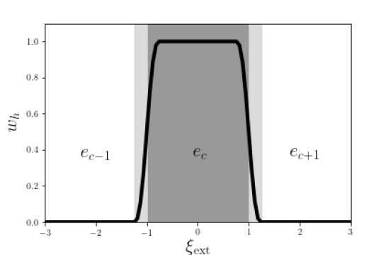
While the Chebyshev smoother is easy to implement, it is reliant on a robust estimate of the largest eigenvalue and this may not be always true in our case. Thus we also implement an additive Schwarz smoother in the manner of Stiller (2017), which is much more robust. The Schwarz smoother works by performing local solves on element-centered subdomains and then adding a weighted sum of these local solves to obtain the smoothed solution. A simple example of one of these subdomains (where the grid is both p and h-uniform) is shown in Figure 4. More generally, the Schwarz subdomain centered on element $e_{c}$ of the mesh is constructed as follows: Starting with all collocation points on $e_{c}$, one adds all boundary points of neighboring elements which coincide with faces, vertices or corners of $e_{c}$. Around these collocation points, one then adds $N_{\rm overlap}-1$ layers of additional collocation points (in Fig. 4, $N_{\rm overlap}=2$). If the mesh has non-uniform $h$ or $p$ refinement, the resulting set of collocation points will have ragged boundaries.

Figure 4: A simple 2-D Schwarz subdomain, with no h-nonconforming or p-nonconforming boundaries. In grey is the element $e$ which is the center of the subdomain. The light grey area is the overlap (of size $\delta_{\xi}$) into the other elements. The subdomain is composed of everything in light and dark grey.

The solutions on the individual Schwarz subdomains are combined as a weighted sum. The weights differ with each collocation point of each subdomain. In 1-D, for a Schwarz subdomain centered on element $e_{c}$ with left and right neighbours $e_{c-1}$ and $e_{c+1}$ we define an extended LGL coordinate $\xi_{\text{ext}}$ for a collocation point $x$ as follows:

$$\xi_{\text{ext}}(\boldsymbol{x})=\begin{cases}\xi^{*}&\boldsymbol{x}\in e_{c},\\ \xi^{*}\pm 2&\boldsymbol{x}\in e_{c\pm 1},\end{cases}$$ (38)

where $\xi^{*}$ is the LGL coordinate of the collocation point $x$ in the reference coordinate system of the macro-element containing $e_{c}$. This definition takes care of the case when a Schwarz subdomain contains a face that is on a tree boundary.

We denote the overlap size as $\delta_{\xi}$ and compute it as the width of the Schwarz subdomain overlap in the coordinate $\xi_{\text{ext}}$. With these definitions we compute the weights for this 1-D subdomain using the function $w_{h}:\mathbb{R}\to\mathbb{R}$ defined as

$$w_{h}(\xi_{\text{ext}})=\frac{1}{2}\left(\phi\left(\frac{\xi_{\text{ext}}+1}{\delta_{\xi}}\right)-\phi\left(\frac{\xi_{\text{ext}}-1}{\delta_{\xi}}\right)\right),$$ (39)

where the $\phi$ function is given by

$$\phi(\xi)=\begin{cases}\text{sgn}(\xi),&|\xi|>1,\\ \frac{1}{8}(15\xi-10\xi^{3}+3\xi^{5}),&|\xi|\leq 1.\end{cases}$$ (40)

We have plotted the weighting function $w_{h}$ in Figure 5.

For Schwarz subdomains in d-dimensions, the weights are computed as a product of 1-dimensional weights along each dimension,

$$W=\prod_{i=1}^{d}w_{h}(\xi^{i}_{ext}).$$ (41)

For the Schwarz subdomain solves we need to define the following operators: $R_{s}$ is the restriction operator for a Schwarz subdomain, it reduces the data on the mesh to the nodes of the subdomain. $R_{s}^{T}$ is the transpose of this operator. $W_{s}$ are the weights for a Schwarz subdomain, computed by evaluating Eq. (39) on the nodes of the subdomain. With these definitions, the Schwarz smoother algorithm is listed in Alg. 6. In Alg. 6, $N_{s}$ indicates the number of smoothing cycles (typically, $N_{s}=3$), $N_{subs}$ indicates the number of subdomains which for our implementation is equal to the number of elements. The linear system on line 6 of Alg. 6 is of the size of the Schwarz-subdomain; we solve it with conjugate gradients to a relative tolerance of $10^{-3}$.

Figure 5: A plot of the Schwarz weighting function defined by Eq. (39). The dark grey shaded region is the center element of the Schwarz subdomain $e_{c}$ and the light grey shaded region is the overlap of width $\delta_{\xi}$. For this plot, we set $\delta_{\xi}=.25$.

Algorithm 6 Schwarz Smoother
$N_{\text{iter,Sch}}$ is a user-defined parameter.

1:function SMOOTHER($x,b,\mathrm{J}$)

2:     for $k=1...N_{\text{iter,Sch}}$ do

3:         $r\leftarrow b-{\rm J}x$

4:         for $s=1...N_{\text{subs}}$ do

5:              $r_{s}\leftarrow R_{s}r$

6:              Solve $R_{s}\mathrm{J}R^{T}_{s}\delta x_{s}=r_{s}$

7:         end for

8:         $x\leftarrow x+\sum_{s}R_{s}^{T}W_{s}\delta x_{s}$

9:     end for

10:     return $x$

11:end function

II.4.6 Multigrid Inter-mesh Operators

Let us now turn to the implementation of restriction and prolongation operators. For clarity, we use the following notation: a superscript lowercase h refers to the children elements and an uppercase H refers to the parent element.

We recall our requirement that the polynomial order of a coarse element is smaller than or equal to the polynomial orders of its children elements (cf. Sec. II.4.3). This ensures that a parent element’s Lagrange polynomial space is always embedded in the broken Lagrange polynomial space of its children. In particular, the coarse-mesh basis-functions can be written, exactly, as

$$\psi_{\alpha}^{H}=(I_{h}^{H})_{\beta\alpha}\psi_{\beta}^{h},$$ (42)

where $(I_{h}^{H})_{\beta\alpha}=\psi_{\alpha}^{H}(\boldsymbol{\xi}^{\beta}_{h})$ is the interpolation-matrix of the coarse-mesh basis-functions to the fine-mesh collocation points, and where we utilized our choice of a nodal basis.

For $h$-refinement, each $\psi_{\beta}^{h}$ has support in only one of the child-elements and, consequently, the implicit sum over $\beta$ in Eq. (42) goes over the basis-elements of all children elements.

The preceding paragraph immediately suggests the natural definition of the prolongation operator from a coarse-grid function $u^{H}\!=\!u^{H}_{\alpha}\psi_{\alpha}^{H}$ to a fine-grid function $u^{h}\!=\!u^{h}_{\beta}\psi_{\beta}^{h}$ such that $u^{h}\equiv u^{H}$. This yields

$$u^{h}_{\beta}=u^{H}(\boldsymbol{\xi}^{\beta}_{h})=(I_{h}^{H})_{\beta\alpha}u^{H}_{\alpha},$$ (43)

so that $(I_{h}^{H})$ represents the prolongation operator.

Because the left hand side operator for the weak equations —e.g. $L(\cdot,\cdot)$ in Eqn. (II.1.2)— is a bilinear form, the residual will also be a bilinear form, which we will denote $B(\cdot,\cdot)$; on the coarse grid. Equation (42) therefore implies

$$B(\,\cdot\,,\,\psi_{\alpha}^{H})=(I_{h}^{H})_{\beta\alpha}B(\,\cdot\,,\psi_{\beta}^{h}),$$ (44)

which defines our coarse grid residual.

Lastly, let us consider restriction of the operators itself. After linearization around the current solution $u_{0}$, the problems we consider here take the form

$$\nabla^{2}\delta u+f(u_{0})\delta u=0,$$ (45)

for some function $f$. The associated weak form reads

$$L_{h}(\delta u,\psi_{\alpha})+\int f(u_{0})\psi_{\alpha}\delta u\,\mathrm{d}\boldsymbol{x}=0\qquad\forall\;\psi_{\alpha}.$$ (46)

The weak Laplacian operator ($L_{h}(\cdot,\cdot)$) can be computed on any coarse grid via Eqn. (II.1.2) without any need for a restriction operator. The second term will require either a restriction operator on $f(u_{0})$, or a restriction operator on $O^{h}_{\alpha\beta}\equiv\int f(u_{0})\psi^{h}_{\beta}\psi^{h}_{\alpha}\mathrm{d}\boldsymbol{x}$. We choose the latter. By Eq. (42), it holds that

$$\int f(u_{0})\psi_{\alpha}^{H}\psi_{\beta}^{H}\,\mathrm{d}\boldsymbol{x}=(I_{h}^{H})_{\gamma\alpha}(I_{h}^{H})_{\delta\beta}\int f(u_{0})\psi_{\gamma}^{h}\psi_{\delta}^{h}\,\mathrm{d}\boldsymbol{x},$$ (47)

so that the restricted operator in matrix form becomes

$$O^{H}=(I_{h}^{H})^{T}\;O^{h}\;(I_{h}^{H}).$$ (48)

II.5 hp-Adaptivity

One of the great advantages of the discontinuous Galerkin method is that it naturally allows for two different methods of refining the grid, h-adaptivity, where one subdivides the element into smaller sub-elements, and p-adaptivity, where one increases the order $p_{e}$ of the polynomial basis on an element. The combination of both h-adaptivity and p-adaptivity is called hp-adaptivity. If one strategically p-refines in smooth regions of the mesh and h-refines in discontinuous regions of the mesh, then it is possible to regain exponential convergence in particular error norms for problems with non-smooth functions. In the next four sections we will discuss the four components of our hp-adaptive scheme. These are: (1) The expected convergence of the solution on a series of adaptively refined hp-meshes (2) an a posteriori error estimator to decide which elements will be refined; (3) a driving strategy that determines based on the convergence of the error estimator whether to h-refine or p-refine; (4) an efficient method to apply discrete operators in multi-dimensions on an hp-grid. We discuss these four items in order in the follow subsections.

II.5.1 Expected Convergence

For quasi-linear problems with piecewise-analytic solutions $u$ on polygonal domains, the convergence of the energy norm (Eq. 33) of the analytical error for the numerical solution $u_{h}$ is

$$||u-u_{h}||_{*}\leq C\left(\sum\limits_{e\in\mathbb{E}}\frac{h_{e}^{2s_{e}-2}}{p_{e}^{2k_{e}-3}}||u||^{2}_{H^{k_{e}}}\right)^{1/2}.$$ (49)

Here ${H^{k_{e}}}$ is the Sobolev space on element $e$ with Sobolev order $k_{e}$ and $1\leq s_{e}\leq\text{min}(p_{e}+1,k_{e})$ Houston et al. (2007, 2008, 2005a); Bi et al. (2015). For uniform refinement and uniform Sobolev order k across elements, we expect $||u-u_{h}||_{*}\leq Ch^{\text{min}(p+1,k)-1}$. Thus, for smooth problems we expect $||u-u_{h}||_{*}\leq Ch^{p}$.

One can show Schötzau et al. (2014) that there exists a series of hp-adaptive refinement steps where the convergence of the energy norm is asymptotically bounded by

$$||u-u_{h}||_{*}\leq C_{1}\exp(-C_{2}\text{DOF}^{1/(2d-1)}).$$ (50)

Here $C_{1}$ and $C_{2}$ are constants, $d$ is the dimension of the mesh and DOF is the number of degrees of freedom, in other words the number of grid points on the mesh.

II.5.2 A Posteriori Error Estimator

Ref. Bi et al. (2015) derives a local a posteriori error estimator for an interior penalty hp-DG discretization of the following class of strongly nonlinear elliptic problems with Dirichlet boundary conditions

$$-\nabla\cdot\boldsymbol{a}(\boldsymbol{x},u,\nabla u)+f(\boldsymbol{x},\nabla u)=0.$$ (51)

The error estimator can be computed locally on each element by the following prescription. Given a discretized solution $u_{h}$, first define quantities on each element $e$ or mortar element $m$ by

$$R_{e} \equiv f(u_{h},\nabla u_{h})-\nabla\cdot\boldsymbol{a}(u_{h},\nabla u_{h}), e\in\mathbb{E},$$ (52a)

$$J_{m,1} \equiv\llbracket\boldsymbol{a}(u_{h},\nabla u_{h})\rrbracket_{m}, m\in\mathbb{M_{I}},$$ (52b)

$$J_{m,2} \equiv\llbracket u_{h}\rrbracket_{m}, m\in\mathbb{M_{I}},$$ (52c)

$$J_{m,3} \equiv\llbracket u_{h}-g_{D}\rrbracket_{m}, m\in\mathbb{M}_{\rm D}.$$ (52d)

From these quantities we compute the followings integrals on an element e and mortar m:

$$\eta^{2}_{e} =h^{2}_{e}p^{2}_{e}||R_{e}||^{2}_{0,e},$$ (53a)

$$\eta^{2}_{m,1} =h_{m}p^{-1}_{m}||J_{m,1}||^{2}_{0,m},$$ (53b)

$$\eta^{2}_{m,2} =\sigma h_{m}^{-1}p^{2}_{m}||J_{m,2}||^{2}_{0,m},$$ (53c)

$$\eta^{2}_{m,3} =\sigma h_{m}^{-1}p^{2}_{m}||J_{m,3}||^{2}_{0,m},$$ (53d)

Here, $||.||^{2}_{0,e}=\int_{e}(.)^{2}\mathrm{d}\boldsymbol{x}=\int_{[-1,1]^{d}}J(.)^{2}\mathrm{d}\boldsymbol{\xi}$ and $||.||^{2}_{0,m}=\int_{m}(.)^{2}\mathrm{d}\boldsymbol{s}=\int_{[-1,1]^{d-1}}S^{m}(.)^{2}\mathrm{d}\boldsymbol{\xi}$. Furthermore, $h_{e}$ is the diameter of the element $e$, $p_{m},h_{m}$ and $\sigma$ are defined in Eq. (32) and $J,S^{m}$ are defined in Eq. (22) and Eq. (23).

Following Bi et al. (2015), we take the local estimator on the element to be

$$\eta^{2}(e)=\eta^{2}_{e}+\sum_{m\subset\mathbb{M}_{e}}\eta^{2}_{m,1}+\sum_{m\subset\mathbb{M}_{e}\setminus\mathbb{M}_{D}}\eta^{2}_{m,2}+\sum_{m\subset\mathbb{M}_{e}\cap\mathbb{M}_{D}}\eta^{2}_{m,3},$$ (54)

where $\mathbb{M}_{e}$ and $\mathbb{M}_{d}$ are the sets of mortar elements touching the element $e$ and $\partial\Omega_{d}$ respectively (see Sec.II.1.1). The estimator provides an estimate of the error in the energy norm, $||u-u_{h}||_{*}$, see Eq. (33). Similar error estimators for various classes of linear and non-linear elliptic PDEs can be found in Houston et al. (2005b); Hansbo and Larson (2011); Zhu et al. (2011); Houston et al. (2007); Schötzau and Zhu (2009); Houston et al. (2005c); Lovadina and Marini (2009). Equations (53) are typically computed on the physical grid on which the elliptic PDE is solved. For highly stretched grids (for instance, when a mapping inverse in radius is used to push the outer boundary to very large radius $R\sim 10^{3}\cdots 10^{10}$), the geometric factors in Eqs. (53) can distort the error estimates. For those cases, we will sometimes introduce a fiducial grid of identical structure and connectivity, that avoids or mitigates excessive grid-stretching. Once a fiducial grid is chosen, its geometric properties can be used in Eqs. (53) and the corresponding norms. Below, we demonstrate that such a “fiducial-grid” error-estimator allows efficient hp-refinement even in highly stretched computational domains. This problem is encountered below in Sec. III.3 and discussed there in greater detail.

II.5.3 Driving Strategy

The a posteriori estimator Eq. (54) indicates which elements to refine. Then the choice must be made for each cell, whether to h-refine or p-refine elements with a large error $\eta(e)$. In the survey paper Mitchell and McClain (2011), Mitchell and McClain looked at 15 different hp-adaptive strategies with a finite elements scheme. Their results indicate that the strategy known as smooth-pred, first introduced in Melenk and Wohlmuth (2001) performs quite well, if not the best under the example problems they tested. For this reason alone we use it, but our code is flexible enough to use any of strategies studied in Mitchell and McClain’s paper.

The idea behind the smooth-pred strategy is based on the observation that for a locally smooth solution, the energy norm Eq. (33) $\eta(e)$ will converge as $h^{p}$, (see Sec. II.5.1). To take advantage of this observation, we first predict the error in the next refinement step and test if this prediction satisfies the smooth error convergence law, if so we p-refine, otherwise we h-refine. The full algorithm is given in Algorithm 7.

Algorithm 7 hp-AMR Driving Strategy
$\gamma_{h}$ and $\gamma_{p}$ are user-defined parameters.

1:procedure SMOOTH-PRED

2:     if $\eta^{2}(e)\text{ is large}$ then

3:         if $\eta^{2}(e)>\eta^{2}_{\rm pred}(e)$ then

4:              h-refine element

5:              $\eta^{2}_{\rm pred}(e_{\textrm{children}})\leftarrow\gamma_{h}\,\big{(}\frac{1}{2}\big{)}^{d}\big{(}\frac{1}{2}\big{)}^{2p_{e}}\eta^{2}(e)$

6:         else

7:              p-refine element

8:              $\eta^{2}_{\rm pred}(e)\leftarrow\gamma_{p_{e}}\eta^{2}(e)$

9:         end if

10:     end if

11:end procedure

In Algorithm 7, $\eta^{2}(e)$ is the square of the error estimator, Eq. (54) of the element under consideration, and $\eta_{\text{pred}}^{2}(e)$ is the predicted error estimator from the last AMR step assuming the solution on the element is smooth. We always start with $\eta_{\rm pred}(e)=0$, so that each element will first be $p$-refined, before $h$-refinement is considered.

The parameters $\gamma_{p}$ and $\gamma_{h}$ influence the behavior of Alg. 7 as follows: As long as the actual $\eta^{2}(e)$ is small compared to the predicted $\eta^{2}_{\rm pred}(e)$ , Line 3 implies continued $p$-refinement. Since Line 8 reduces the predicted $\eta^{2}_{\rm pred}$ by a factor $\gamma_{p}$, this means, that $p$-refinement continues as long as each increment in $p_{e}$ reduces the error-estimator $\eta^{2}(e)$ by a factor $\gamma_{p}$, i.e. as long as exponential convergence is obtained with convergence rate better than $\sqrt{\gamma_{p}}$. If this convergence-rate is not observed, the driver switches to $h$-refinement, and $\gamma_{h}$ begins to matter. In this case, a large $\gamma_{h}$ will preferably switch back to $p$-refinement, whereas a small $\gamma_{h}$ will prefer continued $h$-refinement. All runs shown in the remainder of this paper use $\gamma_{p}=0.1$. The runs differ in $\gamma_{h}$, which is used to tune h- vs p-refinement, and in how many elements are refined in each AMR-iteration, which is used to control how quickly AMR increases the number of degrees of freedom. However for the majority of the runs we find that $\gamma_{h}=0.25$ is a good choice.

In the numerical examples of this paper we use the following two alternatives for the conditional on line 2 of Alg. 7, i.e. to decide which elements should be refined: In the first test-problem, we refine if $\eta^{2}$ is greater than some constant factor times the mean $\bar{\eta}^{2}$ across all elements $e$. This criterion was used in the original description of the hp-AMR scheme (See Melenk and Wohlmuth (2001)). In the remaining problems we refine a percentage of elements with the largest $\eta(e)$. We change criterion because the estimator may vary over orders of magnitude and this variation may change at each refinement step. In such cases, the percentage criterion robustly captures more of the elements with a large estimator than thresholding on a constant times the average estimator). However, the constant factor times the mean method has the advantage that it is computationally cheap and does not require a global sort of the estimator over all cores like the percentage method does. When we use the percentage indicator, we make use of the highly parallel global sort outlined in Feng et al. (2015).

II.5.4 On-the-fly hp Tensor-Product Operations

To solve the elliptic equations with multigrid on grids that are hp-adaptively refined, a large number of different operators must be generated at run-time. In no specific order, we need at least the following linear operators

• interpolation operators on faces, edges and volumes of size $(p^{\prime}+1)\times(p+1)$ in 1-D, where p is the order of the original data and p’ is the order of the new interpolated data

• restriction operators on faces, edges and volumes of size $(p+1)\times(p^{\prime}+1)$ in 1-D, where p’ is the order of the original data and p is the order of the new restricted data

• derivative operator of order p on the reference element, which has size $(p+1)\times(p+1)$ in 1-D.

We can take advantage of the tensor product nature of the reference element in order to efficiently generate these operators on demand. All of the operators listed can be reduced to a tensor product of 1-D operators when applied in $d\geq 2$ dimensions. Upon requiring a certain operator in a calculation, the process is then as follows

1. Check if the 1-D version of the operator has already been computed in the database, if it has been computed, retrieve and goto step 3, if not goto step 2.

2. Compute the 1-D version of the operator and store in the MPI process-local database.

3. Apply the 2-D or 3-D version of the operator on a vector by using optimized Kronecker product matrix vector operation on the nodal vector v: $(A_{1D}\otimes B_{1D})\vec{v}$ for $d=2$, or $(A_{1D}\otimes B_{1D}\otimes C_{1D})\vec{v}$ for $d=3$. Here $A,B,C$ denote the 1-D matrices of the respective operator, as applied to the first, second, and third dimension.

A Kronecker product matrix vector operation can be efficiently performed using a series of BLAS matrix-multiply calls, see Buis and Dyksen (1996) for example.

II.6 Implementation

To implement the multi-block adaptive mesh refinement we use the p4est library, which has been shown to scale to $\mathcal{O}$(100,000) cores Burstedde et al. (2011). We use PETSc Balay et al. (2001) for the Krylov subspace linear solves and the Newton Raphson iterations. The components of the multigrid algorithm are written by the authors and do not use PETSc.

III Test Examples

We examine the components of our code through three test examples, the first a linear Poisson problem solved on a square grid where the solution is only C²-smooth at the $(0,0)$ grid point. The second example is a non-linear elliptic problem, where we solve the Einstein constraint equations for the initial data of a constant density star. We then end the test examples section with a linear problem on a cubed-sphere with stretched outer boundary and a solution that falls off as $r^{-1}$ with radial coordinate r as $r\rightarrow\infty$. Each test is aimed at isolating different aspects of the puncture black-hole problem, whose solution contains points that are C²-smooth and falls off as $r^{-1}$. The puncture black-hole problem further requires us to solve nonlinear Einstein constraint elliptic equations on a cubed-sphere mesh.

III.1 Poisson with $H^{4-\epsilon}$ solution

The first test problem we will investigate numerically is taken from Stamm and Wihler (2010), where the authors solve $\nabla^{2}u=f$ on $\Omega=(0,1)^{2}$ with the solution chosen as

$$u=x\left(1-x\right)y\left(1-y\right)\left[\left(x-\frac{1}{2}\right)^{2}+\left(y-\frac{1}{2}\right)^{2}\right]^{3/2}.$$ (55)

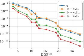
Here $u\in H^{4-\epsilon}$, where $\epsilon>0$ so from Eq. (49) we expect third order convergence for uniform refinement. We have confirmed this numerically. However, with hp-adaptivity, it is possible to achieve $||u-u_{h}||_{*}\sim\exp(\text{DOF}^{\frac{1}{3}})$, as we show in Fig. 6. Notice also the close agreement between the estimator and energy norm $||u-u_{h}||_{*}$. The final mesh is shown in Fig. 7. Of note is the fact that the elements with the lowest polynomial order (p=4) are only in the vicinity of the $C^{2}$-smooth $(0,0)$ grid-point and the refinement level of the mesh is locally much higher here as well. Here we used AMR parameters $\gamma_{h}=10$, $\gamma_{p}=0.1$; at each AMR iterations all cells were refined which have $\eta^{2}(e)$ larger than $1/4$ of the overall mean of all $\eta^{2}(e)$. For this problem, we performed a survey of different choices for $\gamma_{h}$ and $\gamma_{p}$. We found rather modest dependence on $\gamma_{h}$ within $0.25\lesssim\gamma_{h}\lesssim 10$, with $\gamma_{h}\!=\!10$ leading to the good balance between $h-$ and $p-$refinement shown in Fig. 7. Our preferred value for the rest of the paper ($\gamma_{h}=0.25$) also yields good convergence, but leads to a more uniform polynomial degree through the mesh.

Figure 6: Problem A, Eq. (55): Convergence of the energy norm estimator $\eta^{2}$ and the error between the numerical solution $u_{h}$ and the analytic solution $u$ in the energy norm $||\cdot||_{*}$ (Eq. 33) and the $L_{2}$ norm $||\cdot||_{2}$ (Eq. 34).

Figure 7: Problem A, Eq. (55): Visualization of the solution and the hp-refined computational mesh. Top portion: The computational grid, color-coded by polynomial degree, with height representing the solution $u$. Bottom portion: Color-coded by $h$-refinement level. A cell on level $l$ has size $2^{-l}$ of the overall computational domain.

Figure 8: Problem A, Eq. (55): Iteration-count of the flexible conjugate gradient (FCG) Krylov subspace solver versus the Multigrid preconditioned FCG solver (MG-FCG). The MG-FCG completes all solves in $\leq 3$ iterations.

III.2 Constant density star

For the next test problem, taken from  Baumgarte et al. (2007), we solve the Einstein constraints in the simplest possible scenario, a constant density star. The goal of this test problem is to investigate how the elliptic solver behaves for problems that contain surface discontinuities that mimick surface and phase transition discontinuities in a Neutron star. The Einstein constraint equations for the case of a constant density star reduce to

$$\nabla^{2}\psi+2\pi\rho\psi^{5}=0,$$ (56)

where $\rho$ is the density of the star and $\psi$ is the conformal factor which describes the deviation of the space from flat space. In Baumgarte et al. (2007) the authors solve the above equation for the case of a star with radius $r_{0}$ and mass-density

$$\rho=\begin{cases}\rho_{0}&r\leq r_{0}\\ 0&r>r_{0},\end{cases}$$ (57)

where r is the radial spherical polar coordinate. Since the star is in isolation, the boundary condition at infinity is $\psi=1$, corresponding to a asymptotically-flat space. For such a problem, there is an analytic solution given by

$$\psi=\begin{cases}Cu_{\alpha}(r)&r\leq r_{0}\\ \frac{\beta}{r}+1&r>r_{0}.\end{cases}$$ (58)

with $C=(2\pi\rho_{0}/3)^{-1/4}$ and

$$u_{\alpha}(r)\equiv\frac{(\alpha r_{0})^{1/2}}{(r^{2}+(\alpha r_{0})^{2})^{1/2}}.$$ (59)

The parameters $\alpha$ and $\beta$ are determined from the continuity of $\psi$ and it’s first derivative at the surface of the star, and are given by

$$\beta=r_{0}(Cu_{\alpha}(r_{0})-1)$$ (60)

$$\rho_{0}r_{0}^{2}=\frac{3}{2\pi}\frac{\alpha^{10}}{(1+\alpha^{2})^{3}}$$ (61)

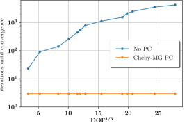
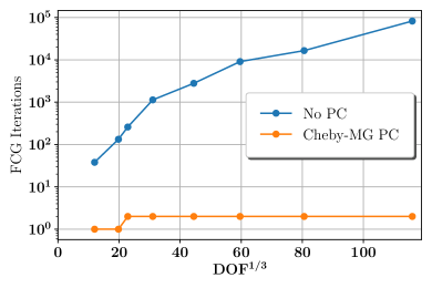
We solve the above problem on a cubic domain with $\rho_{0}=0.001$ and analytic Dirichlet boundary conditions on a boundary at $8r_{0}$. The non-linear term in Eqn. 56 is handled by first interpolating $\psi$ onto the GL quadrature points of an element, evaluating $\psi^{5}$ at the GL quadrature points and then performing the necessary Gaussian quadrature sum on each element. Figure 9 showcases the convergence of the solution and the nice agreement between the energy norm estimator $\eta^{2}$ and the energy norm of the analytic error. To achieve this convergence we used the following AMR parameters, $\gamma_{h}=0.25$, $\gamma_{p}=0.1$. At each AMR refinement iteration, 10% of the elements are refined. In Figure 10 we show a comparison between multigrid-preconditioned FCG iterations and unpreconditioned FCG iterations. We notice that for the preconditioned case, the iteration count is roughly constant with increases in DOF, whereas the unpreconditioned iterations grow with DOF. Finally, in Figure 11 we show the mesh after the last AMR step. This mesh showcases the highest h-refinement around the star boundary (yellow circle) as expected, since this area is not smooth.

Figure 9: Problem B, Eq. (56): Convergence of the energy norm estimator $\eta^{2}$ and the error between the numerical solution $u_{h}$ and the analytic solution $u$ in the energy norm $||\cdot||_{*}$ and the $||\cdot||_{2}$ norm

Figure 10: Comparison of the average number of iterations per Newton-Raphson step when using a Chebyshev smoothed Multigrid preconditioner and no preconditioner.

Figure 11: Visualization of hp-refined computational mesh for Problem B, Eq. (56). Top portion: The $z=0$ cross-section of the computational grid, color-coded by the polynomial degree and with height representing the solution $\psi$. Bottom portion: Volume rendering of the $z\leq 0$ part of the computational domain, color-coded by the $h$-refinement level. A cell on level $l$ has size $2^{-l}$ of the overall computational domain.

III.3 Cubed sphere Meshes and Stretched Boundary Elements

Figure 12: The mesh structure for a computational domain with spherical outer boundary. This structure consists of 13 macro-meshes (shown in different colors). For clarity, only the $z\leq 0$ part of the mesh is shown.

So far, we have only investigated meshes with a regular, Cartesian structure and with a rectangular outer boundary at close distance. We will now investigate scenarios with a spherical outer boundary, where we use a macro-mesh arising from the 3-dimensional generalization of Fig. 1 (a). We will also place the outer boundary at very large radius, typically $10^{9}$, to approximate boundary conditions at infinity. Typically, such problems have solutions which fall off as a power series in $1/r$.

Figure 12 shows the structure of the mesh we will use: a central cube, surrounded by two layers of six deformed macro-elements each. The inner layer interpolates from the cubical inner region to a spherical outer region. The outer layer has spherical boundaries both at its inner and outer surface, and thus radial coordinate lines that are always orthogonal to the angular coordinate lines. This allows to apply a radial coordinate transformation in the outer layer, to move its outer boundary to near infinity. Because we know the solution will fall off as $1/r$ we use an inverse mapping in the outer six spherical wedges of the cubed-sphere (blocks 0-5 in Fig. 12). This mapping is defined as follows. Denote the physical grid variable with $r\in[r_{1},r_{2}]$ and the collocation-point integration variable as $x\in[x_{1},x_{2}]$, then the inverse mapping is defined by

$$r=\frac{m}{x-t},$$ (62)

where

$$m=\frac{x_{2}-x_{1}}{\frac{1}{r_{2}}-\frac{1}{r1}},\qquad t=\frac{x_{1}r_{1}-x_{2}r_{2}}{r_{1}-r_{2}}.$$ (63)

We will investigate the discontinuous Galerkin method on the following test problem which captures many of the above features:

$$\nabla^{2}u=3(1+x^{2}+y^{2}+z^{2})^{-\frac{5}{2}},$$ (64)

with $\Omega=\{(x,y,z):x^{2}+y^{2}+z^{2}<R\}$ and Dirichlet boundary conditions given by the analytical solution, which is a Lorentzian function $u=(1+r^{2})^{-1/2}$. The Lorentzian function falls off as a power series in $1/r$ as $r\rightarrow\infty$.

To solve this test problem we run two schemes: uniform $p$-refinement and adaptive p-refinement. We run only with p-AMR because the underlying solution is smooth everywhere so there is very little to no benefit in running with hp-AMR for this problem (which we also found to be the case empirically). For the uniformly refined run, we start with refinement level $l=4$, i.e. with $2^{3l}=4096$ elements in each of the 13 macro-elements, and increase $p$ from $2$ to $11$.

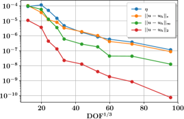
To achieve pure p-AMR with the hp-AMR scheme outlined in Sec. II.5, we start with refinement level $l=2$, i.e. with $2^{3l}=64$ elements in each of the 13 macro-elements, and with polynomial order $p_{e}=1$ in all elements. We set $\gamma_{h}\!=\!10^{6}$, $\gamma_{p}\!=\!10^{6}$ and in each AMR iteration, we refine the $25\%$ elements with the largest estimator. Figure 13 shows the convergence of the p-AMR scheme versus the p-uniform scheme. We stop at the maximum polynomial order currently allowed in the code, $p\!=\!19$. Comparing the $L_{\infty}$ norm between the p-AMR and p-uniform runs, the number of degrees of freedom per dimension, $\mbox{DOF}^{1/3}$, is roughly cut in half. The $L_{2}$ norm is slower to converge because it is dominated by the contributions of the outer stretched wedges, and this region is less aggressively refined by the AMR. Figure 14 shows the final mesh for the problem. The AMR algorithm increases the polynomial order $p$ predominantly in the centre, where the solution has the most structure.

Figure 13: Problem C, Eq. (64): Convergence of the solution as the degree p is uniformly increased across all elements for uniform case and as the degree p is adaptively increased in the amr case. (Dirichlet BC at R=1000).

Figure 14: Visualization of the final mesh for problem C. Shown is a xy-plane slice of the mesh which has been warped so that the height of the surface corresponds to the value $u$ of the solution, color coded by the polynomial degree. For ease of visualization, grid-points are mapped onto the compactified grid on which the estimator $\eta_{e}$ is computed; the compactified outer radius $R=3$ corresponds to the physical outer radius $R=1000$.

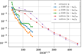
Strong coordinate stretching, as performed via the inverse map Eq. (62) leads to the following problem: The error estimator $\eta^{2}(e)$ utilizes integrals in physical coordinates in Eqs. (52). For strongly stretched grids (e.g. with inverse mappings where $R$ is orders of magnitude larger than other length scales in the problem) these volume integrals will place a large emphasis on the regions at large distance. AMR will then aggressively refine in the stretched region despite the pointwise errors (as measured by the $L_{\infty}$ norm for individual elements) being very small. Such regions tend to have a very low $L_{\infty}$ because the numerical solution is very accurate there, but a high $L_{2}$ because of the large volume in the stretched region, thus also explaining why the $L_{2}$ norm of the p-AMR run in Fig. 13 fails to converge as smoothly as the $L_{\infty}$ norm.

We solve this problem by introducing a “compactified grid”, which has the same structure as the physical grid, but without the compactification in the physical grid. We then compute the integrals for the estimator in Eqs. (53) on this compactified grid. The integrands, Eqs. (52), are as before computed on the physical grid. In essence, this procedure merely changes the weighting of the different regions of the grid via the Jacobians $J$ in the integrals and the parameters $h_{e},h_{m}$ which are now computed on the compactified grid. In practice, we use as compactified grid a cubed-sphere mesh where the outer spherical shell extends from radius $2$ to radius $3$, and where the middle cube has a side-length of $2/\sqrt{3}$.

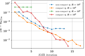
Figure 15 shows the convergence of the $L_{\infty}$ norm using the compactified grid versus the non-compactified grid. For $R=1000$, the standard estimator (“non-compact $\eta$”) converges well for the first 10 AMR iterations, but then stalls. For $R=10^{9}$, the standard estimator fails to yield convergence of the solution at all. For both cases, the new estimator (“compact $\eta$”) results in good convergence. We stress that the compactified estimator is only used in driving the AMR refinement. The DG-scheme is always formulated in the physical domain, and also the error plotted in Fig. 15 is computed from the solution on the physical domain with outer boundary $R=1000$ or $10^{9}$. The p-AMR run shown in Fig. 13 uses the compactified estimator.

Figure 15: Problem C, (Eq. 64): Convergence of the solution in the $L_{2}$ norm (See Eq. 34) as the degree p is adaptively refined with a compact and non-compact estimator. (Dirichlet BC at R=1000 and $R=10^{9}$). All runs use the AMR/dG parameters of the p-amr run in Figure 13.

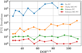
Finally, we investigate the efficiency of preconditioners for the p-AMR run with $R=1000$ and the compactified estimator, i.e. the run plotted in orange in Figs. 13 and 15. Figure 16 presents the iteration counts for four different kinds of preconditioning. Chebyshev-smoothed multigrid preconditioner loses efficiency on cubed spheres with stretched boundaries, possibly due to a poorly estimated upper eigenvalue in Alg. 5. However, using the more powerful domain decomposition additive Schwarz method, we can regain the efficiency of the multigrid-preconditioner seen in the previous two sections. Here, the Schwarz subdomains have $N_{\rm overlap}=2$, and each multi-grid iteration employs $N_{\rm iter,Sch}=3$ iterations of Schwarz-smoothing with rtol=1e-3. Chebyshev uses $N_{\rm iter,eigs}=15$ iterations for the eigenvalue estimate, and $N_{\rm iter,Cheb}=15$ iterations in the Chebyshev smoother.

Figure 16: Comparison of four different methods of preconditioning FCG. All runs use the AMR/dG parameters of the p-amr run in Figure 13.

III.4 Puncture Initial Data

There are various approaches to solving for binary black hole initial data sets and these approaches are primarily distinguished by the initial choice of hypersurface and how the physical singularity inside the black holes is treated. One possibility when considering two black holes is to work on $\mathbb{R}^{3}$ with two balls excisedCook (1994); Cook and Pfeiffer (2004); Caudill et al. (2006). This approach has been shown to work well with the spectral finite element method (e.g. Pfeiffer et al. (2003b)), but is more problematic for finite-difference codes because special stencils must be created near the curved boundaries. Another popular approach, which is more amenable to finite difference codes is the puncture method Brandt and Brügmann (1997), where an elliptic equation is solved on $\mathbb{R}^{3}$, with two points where the solution becomes singular. These points represent the inner asymptotically flat infinity (Brill-Lindquist topology). The puncture method simplifies the numerical method because no special inner boundary condition has to be considered, however the solution is only $C^{4}$ smooth at the puncture points Brandt and Brügmann (1997). Without using contrived coordinate systems to remove the $C^{4}$-smooth nature of the punctures (See Ansorg et al. (2004) for example), spectral methods cannot perform optimally, because they would require the solution to be smooth on the computational domain in order to obtain exponential convergence. We choose to solve for binary black hole initial-data with the puncture method in this paper for two reasons. The first is that the method does not couple well with traditional spectral schemes as discussed above and this allows us to compare the discontinuous Galerkin method to the spectral method. Secondly, the equation we must solve is less complicated than the excision case because it only involves a solve for a single field, the conformal factor, as opposed to the 5 fields one must solve for with the excision method (see e.g. Pfeiffer et al. (2003b)), so it is easier to implement numerically.

Nevertheless, puncture data provides a testing ground for many of the new techniques developed here: Singular points which benefit from h-refinement; smooth regions that benefit from p-refinement; a spherical outer boundary requiring the cubed-sphere domain shown in Fig. 12; and a boundary at infinity (or near infinity) which requires a compactified radial coordinate. Moreover, for testing of adaptivity, it is easy to add arbitrarily many black holes each represented by its own singularity, at arbitrary coordinates with arbitrary spins.

For the case of puncture data, the initial data equations of general relativity reduce down to a single equation Brandt and Brügmann (1997):

$$-\nabla^{2}u=\frac{1}{8}\bar{A}^{ij}\bar{A}_{ij}\psi^{-7}$$ (65)

where $\bar{A}_{ij}$ is a spatially dependent function given by

$$\bar{A}_{ij}=\frac{3}{2}\sum_{I}\frac{1}{r^{2}_{I}}[2P^{I}_{(i}n^{l}_{j)}-(f_{ij}-n^{l}_{i}n^{l}_{j})P^{k}_{I}n^{I}_{k}+\frac{4}{r_{I}}n^{l}_{(i}\epsilon_{j)kl}S^{k}_{I}n^{l}_{I}].$$ (66)

Here, $n^{i}_{I}$ are the spatially varying components of the radial unit-vector $\hat{n}_{I}(\vec{x})=(\vec{x}-\vec{c}_{I})/|\vec{x}-\vec{c}_{I}|$ relative to the position $\vec{c}_{I}$ of the $I$-th black hole Brandt and Brügmann (1997). The constant vectors $\boldsymbol{P}_{I}$ and $\boldsymbol{S}_{I}$ quantify the momentum and spin of the $I$-th black-hole and $\psi=1+\sum_{I}\frac{m_{I}}{2r_{I}}+u$. The boundary condition is

$$u\to 0,\quad|\vec{x}|\to\infty.$$ (67)

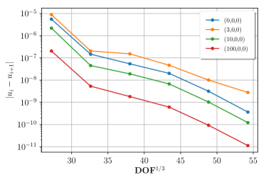
We solve the above elliptic PDE using first the spectral code SpEC and then the dG solver presented in this paper. We solve for the case of two orbiting equal mass black holes with momenta $\pm.2$, zero spin and initial positions $(\pm 3,0,0)$ in units of total mass M. This is the test case used in Ansorg (2007). Since there is no analytical solution, we will compare the solutions between refinement levels at four reference points on the x-axis. These are $(0,0,0)$, $(3,0,0)$, the location of the right-most puncture, $(10,0,0)$ and $(100,0,0)$.

The SpEC solver was already used to solve for puncture data in Dennison et al. (2006); Lovelace et al. (2008). This spectral code is apriori not well suited for puncture data which results in a non-smooth solution $u(\vec{x})$. Because we know where the singularities of the punctures are, this can be overcome manually, by covering the punctures with very small rectangular blocks, at high enough resolution, to compensate for the loss of exponential convergence. Figure 17 shows the difference in the solution at the four reference points as the resolution is manually increased. We emphasize that this solution obtained with SpEC depents on (i) prior knowledge of the locations of the singularities; and (ii) tuning of SpEC’s mesh and resolution by hand.

Figure 17: Convergence of the SpEC–elliptic solver with manually adopting the domain-decomposition and manual adjustment of resolution to compensate for the singularities. Plotted are differences to the next-lower resolution at four points in the computational domain.

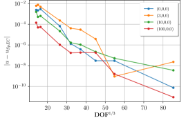
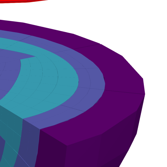
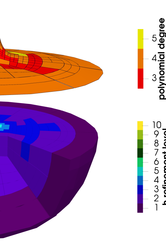
For the dG solver, we start with a uniformly refined cubed-sphere mesh at level $l=1$, i.e. 13 blocks, each consisting of eight cells. The outer radius at $10^{11}$M and the size of the inner cube is 10M. We start further with elements of polynomial order $p=2$. The location of the punctures is not utilized in the dG code, and all mesh-refinement is automatic, driven by Alg. 7 with parameters $\gamma_{h}=.25$ and $\gamma_{p}=.1$ and we refine the top $12.5\%$ of elements. In order to run a Schwarz smoother for this problem we would need to transfer ghost-data for the operator described by Eqn. (48) whenever a Schwarz subdomain contains a ghost element. While this is by no means problematic, we have not yet implemented the infrastructure to do it, so we just use a Chebyshev smoother when we precondition this problem with Multigrid. Figure 18 shows the convergence of the four reference points with respect to the finest grid SpEC solution between AMR levels. We first see that in terms of overall DOF, the dG solver doesn’t do much worse than the finely tuned SpEC solver, even though the dG solver has to adaptively find the punctures, has a larger initial error and has no h-or-p coarsening, so mistakes in the refinement cannot be fixed. Thus, taken all of this into account, the convergence is highly satisfactory. The bounce in the $(3,0,0)$ at the second to last iteration arises because the dG-solution oscillates around the SpEC solution and coincidentally is shown near a zero-crossing. Figure 20 shows the solution on the final mesh, which has the highest h-refinement exactly at the points of the punctures, as desired.

Figure 18: Problem D: Black hole initial data with two punctures. Convergence of the error between the dG solution and the SpEC solution.

Figure 19: Problem D (Black hole initial data with two punctures): Visualization of the hp-refined computational mesh. The bottom portion of the image shows a volume rendering of the $z<0$ portion of the computational domain, with two blocks removed, and color-coded by the h-refinement level. The top portion of the image shows the $z=0$ cross-section of the computational grid, color-coded by the polynomial degree, with the height representing the solution $u$. For ease of visualization, grid-points are mapped onto the compactified grid on which the estimator $\eta_{e}$ is computed; the compactified outer radius $R=3$ corresponds to the physical outer radius $R=10^{11}$.

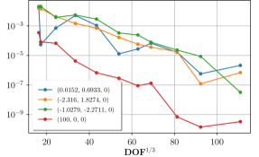
Next, we solve for the puncture initial data of three black-holes randomly located in the xy-plane, with random spins and random momenta. Spectral solvers such as SpEC cannot perform well when the singular points on the grid are not known in advance. Thus, we end this paper showcasing a problem that our discontinuous Galerkin code can solve, but SpEC cannot. Table 1 illustrates the parameters for the randomly placed punctures and their spin and momenta.

Figure 20: Problem E (Black hole initial data with three punctures): Visualization of the solution, and the hp-refined computational mesh. Top portion: the $z=0$ cross-section of the computational grid, color-coded by the polynomial degree, with the height representing the solution $u$. Middle portion: volume rendering of the $z<0$ part of the computational domain, with two blocks removed, and color-coded by the h-refinement level. Bottom portion: Zoom into the middle portion, highlighting the region near the three punctures with highest refinement level. For ease of visualization, grid-points are mapped onto the compactified grid on which the estimator $\eta_{e}$ is computed; the compactified outer radius $R=3$ corresponds to the physical outer radius $R=10^{11}$.

	Puncture 1	Puncture 2	Puncture 3
$m$	0.2691	0.4063	0.3245
$x$	0.0152	-2.316	-1.0279
$y$	-0.6933	1.8274	-2.2711
$P_{x}$	0.0585	-0.0284	0.1640
$P_{y}$	0.0082	-0.1497	0.0515
$S_{z}$	-0.0134	-0.0332	-0.0708

Table 1: The randomly generated parameters for the three black holes. We list the mass m, the position $(x,y,0)$, the momentum $(P_{x},P_{y},0)$ and the spin $(0,0,S_{z})$ of the black holes.

Figure 21 shows the convergence of four points, three at the location of the punctures, and one at $(100,0,0)$. We use amr parameters $\gamma_{h}=0.25$, $\gamma_{p}=0.1$, $F_{\rm refined}=0.125$ for this run.

Figure 21: Problem D: Black hole initial data with three randomly generated punctures. Convergence of the error between AMR steps at four different points, three corresponding to the location of the punctures and one at $(100,0,0)$.

IV Conclusion and Future Work

We presented a new code for solving elliptic equations intended for numerical relativity. The methodology we use differs from other codes in the field in many important respects. In particular, we use a discontinuous Galerkin method to discretize the equations, an hp-adaptive mesh refinement scheme driven by an a posteriori estimator and a matrix-free, scalable Multigrid preconditioned Newton-Krylov solver. Individually, many of the features of our code have been implemented before Kozdon and Wilcox (2018); Kozdon et al. (2019); Stiller (2017); Sundar et al. (2012); Hesthaven and Warburton (2008), but they have never been combined together to create a general dG solver. In particular, the combination of curved meshes (cf. Fig. 12) and non-conforming elements is novel and is crucial for generic solution-driven AMR. Moreover, the compactified AMR-driver introduced in Sec. III.3 is also new, enabling AMR on compactified computational domains with outer boundary near infinity. Lastly, the use of a multigrid-preconditioned solver with a Schwarz (or Chebyshev) smoother on non-polygonal meshes has not been investigated in a dG setting until this paper.

For BBH puncture data, our new code approaches the accuracy of existing, specialized codes like SpEC. In addition, the automatic AMR in the new code does not require manual tuning of the computational mesh, and does not utilize any prior knowledge of features of the solution like the location of black hole punctures. The new code already improves on the more specialized codes by being able to handle an arbitrary number of puncture-black holes. AMR can also automatically resolve discontinuities without prior knowledge of their existence (cf. Fig. 11).

Moving forward, there are still several areas of improvement our code could possibly benefit from:

1. Load balancing: For problems that require adaptive mesh refinement and multi-grid, there will naturally be a unbalanced number of degrees of freedom (DOF) across processors and this can slow down the Krylov iterations substantially. This can be amended by incorporating a task-based parallelism framework for load balancing. The elliptic solver developed in this article will be incorporated task-based parallel code SpECTRE, which is concurrently being developed Kidder et al. (2017).

2. Anisotropic refinement: Most realistic problems have some anisotropy and therefore a solver would benefit from anisotropic mesh refinement. Indeed, most of the problems in this paper could have had better convergence with anisotropic refinement, for instance, Problem C is spherically symmetric, and puncture data is approximately spherically symmetric at large distance. We use the p4est framework for mesh refinement and while it has support for anisotropic refinement, the direction of the anisotropy has to be known a priori. We look to go beyond this and have general refinement in a future edition of our code.

3. Hybridizable dG: The discontinuous Galerkin method can be quite expensive in terms of the amount of DOF it requires to converge to a certain error. Recently, a method called Hybridizable dG has been coupled with matrix-free multigrid methods to solve elliptic problems with substantially reduced DOF over the classical dG method Fabien et al. (2019); Muralikrishnan et al. (2019). Whether this method can be fully incorporated into the complex scheme presented in this paper, will be an area of further inquiry.

In future work, we plan to use this solver to expand the physics in compact object initial data, for instance, neutron star initial data for equation of state with phase-transitions, neutron stars with very high compactness (where current solvers fail Henriksson et al. (2016)), or compact objects in alternative theories of gravity, or with novel matter fields like boson stars.