Classification of Cardiac Arrhythmias from Single Lead ECG
with a Convolutional Recurrent Neural Network

Abstract

While most heart arrhythmias are not immediately harmful, they can lead to severe complications. In particular, atrial fibrillation, the most common arrhythmia, is characterized by fast and irregular heart beats and increases the risk of suffering a stroke. To detect such abnormal heart conditions, we propose a system composed of two main parts: a smart vest with two cooperative sensors to collect ECG data and a neural network architecture to classify heart rhythms. The smart vest uses two dry bi-electrodes to record a single lead ECG signal. The biopotential signal is then streamed via a gateway to the cloud where a neural network detects and classifies the heart arrhythmias. We selected an architecture that combines convolutional and recurrent layers. The convolutional layers extract relevant features from sliding windows of ECG and the recurrent layer aggregates them for a final softmax layer that performs the classification. Our neural network achieves an accuracy of 87.50% on the dataset of the challenge of Computing in Cardiology 2017.

1 INTRODUCTION

Heart arrhythmias are caused by irregular electrical conduction in cardiac tissue. Atrial fibrillation, which affects 1–2% of the population [Camm et al., 2010], is the most common one. Furthermore, its prevalence increases with age, from $<$0.5% at 40–50 years to 5–15% at 80 years. While not directly life-threatening, it can lead to serious complications [January et al., 2014]. In particular, atrial fibrillation is associated with a 3–5 fold increased risk of stroke and a 2-fold increased risk of mortality [Kannel et al., 1998]. It is also associated with a 3-fold risk of heart failure [Wang et al., 2003]. Typical symptoms include heart palpitations, shortness of breath, and fainting. However, about one third of the cases are asymptomatic which prevents early diagnosis. This, in turn, precludes early therapies which might protect the patient from the consequences of atrial fibrillation but also from its progression. Indeed, atrial fibrillation causes electrical and structural remodeling of the atria which facilitates its further development [Frick et al., 2001, Nattel et al., 2008].

The gold standard for diagnosing atrial fibrillation and other heart arrhythmias is the 12-lead ECG. A trained electrophysiologist can select the most appropriate treatment after reviewing ECG signals and the patient history. This is, however, a time-consuming task, especially for long recordings such as the ones collected with Holter monitors. To alleviate this task, several approaches have been proposed to detect arrhythmias from ECG signals [Owis et al., 2002, De Chazal et al., 2004]. Even without perfect detection accuracy, these approaches are useful as they facilitate reviewing ECG by selecting relevant signal excerpts.

Recently, neural networks have shown impressive performance in various classification and regression tasks. Image processing was the first field where deep networks surpassed existing approaches by a large margin [Krizhevsky et al., 2012]. Since then, they have been extensively applied to fields previously dominated by signal processing. In particular, several architectures have been proposed to detect and classify heart arrhythmias from ECG signals.

In the context of the challenge of Computing in Cardiology 2017 [Clifford et al., 2017], a few neural network architectures were proposed to classify single lead ECG signals into one of the following classes: normal sinus rhythm, atrial fibrillation, other rhythm, and noise. One of these architectures uses logarithmic spectrograms computed over sliding windows of ECG as input to two-dimensional convolutional layers [Zihlmann et al., 2017]. Aggregation of successive windows is done with either temporal averaging or a recurrent layer. However, the convolutional and recurrent layers were trained separately due to convergence issues. A similar approach used a 16-layer convolutional neural network with skip connections to classify arrhythmias from ECG signals [Xiong et al., 2017]. Each layer is composed of batch normalization, ReLU activation, dropout, one-dimensional convolution, and averaging pooling.

Recently, a convolutional neural network was shown to reach cardiologist-level arrhythmia detection [Rajpurkar et al., 2017]. This 34-layer network takes advantage of a very large dataset of 64,121 ECG signals, recorded from 29,163 patients, to recognize 12 different heart arrhythmias including atrial fibrillation, atrial flutter, and ventricular tachycardia. Another approach applied convolutional neural networks for detecting atrial fibrillation from time-frequency representations of ECG signals [Xia et al., 2018]. Two methods for computing these representations were compared: the short-time Fourier transform or the stationary wavelet transform. In this case, the neural network using coefficients from the second transform yielded better classification accuracy.

Neural networks have thus shown promising results for the detection of abnormal cardiac rhythms. Furthermore, as mentioned previously, it is of the utmost importance to detect arrhythmias as early as possible to improve treatment outcome. To tackle this issue, we developed a system composed of two main elements: a smart vest to record ECG signals and an algorithm to detect and classify arrhythmias. The smart vest includes two cooperative sensors to record a single lead ECG signal and stream by Bluetooth the collected data to a gateway. This gateway then forwards the ECG signal to the cloud where it is processed by a neural network in order to detect abnormal rhythms.

This article is structured as follows. First, the dataset of ECG signals, our neural network architecture, and the monitoring system are described in Section 2. Then, the results are presented in Section 3 and discussed in Section 4. Finally, this article ends with a short conclusion in Section 5.

2 MATERIALS AND METHODS

2.1 Dataset

We used the dataset from the challenge of Computing in Cardiology 2017 to train a neural network to classify cardiac arrhythmias. This dataset includes 8528 single lead ECG signals recorded with an AliveCor device. The signals are sampled at 300 Hz and have durations ranging from 9 to 60 seconds. Each signal was acquired when the subject held each one of the two electrodes in each hand resulting in a lead I (left arm – right arm) ECG. As the device has no specific orientation, many signals are inverted (right arm – left arm).

All ECG signals are labeled with one of the following four classes: normal sinus rhythm, atrial fibrillation, other rhythm, and noise. The proportion of each class in the dataset varies from 3.27% for noise to 59.52% for normal rhythm. The full breakdown of all classes is reported in Table 1.

Table 1: Number of signals and mean duration for each class.

Class	Count	Proportion	Mean duration [s]
Normal rhythm	5076	59.52%	32.11
Atrial fibrillation	758	8.89%	32.34
Other rhythm	2415	28.32%	34.30
Noise	279	3.27%	24.38
Total	8528	100%	32.50

The entries of the challenge of Computing in Cardiology 2017 were ranked according to the following score evaluated on a private test set:

$$S_{\text{CinC}}=\frac{F_{1n}+F_{1a}+F_{1o}}{3}$$ (1)

where $F_{1n}$, $F_{1a}$, and $F_{1o}$ denote the $F_{1}$ scores for normal rhythm, atrial fibrillation, and other rhythm. The four winners [Teijeiro et al., 2017, Datta et al., 2017, Zabihi et al., 2017, Hong et al., 2017] reached a score of 0.83.

Several aspects of this dataset are challenging for arrhythmia classification. First, many signals are inverted as mentioned previously. Second, the classes are not balanced. There are very few signals labeled atrial fibrillation or noise compared to the ones labeled normal rhythm. Furthermore, the durations of the recordings are also different. They vary from 9 to 60 seconds. Figure 1 illustrates this issue. Most ECG signals last 30 seconds but a significant portion has shorter or longer durations. In addition, labeling is relatively coarse as a single label is associated with each ECG signal. In some cases, several labels could be used for the same signal. Finally, the ECG quality of a non-negligible part of the records is rather poor. Four examples of signals are shown in Figure 2. The first two signals are labeled normal rhythm and atrial fibrillation and have good overall quality. The third example is a normal rhythm record with acceptable quality except for a short segment of noise. The last ECG signal is labeled as atrial fibrillation but has very poor quality due to large shifts of the baseline. It also illustrates that all signals do not share the same duration.

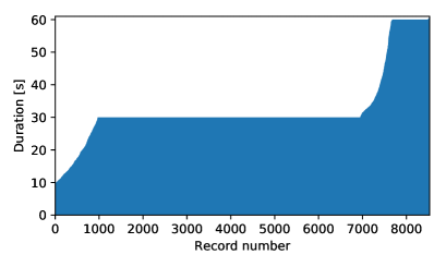
Figure 1: Record durations sorted in increasing order.

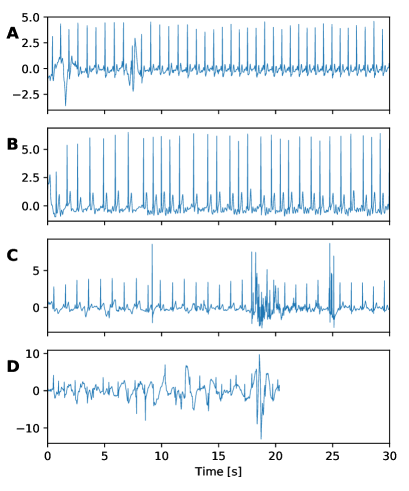
Figure 2: Examples of ECG records: (A) normal rhythm from record A00001, (B) atrial fibrillation from record A00004, (C) normal rhythm from record A00002, (D) atrial fibrillation from record A00015.

The test set used during the challenge of Computing in Cardiology was not yet publicly released. Therefore, we split the dataset (which was originally intended only for training) into a training set of 7000 records and a test set with the remaining 1528 records while approximately preserving class repartition.

We applied the following pre-processing steps to the dataset. First, we filtered the ECG signals with a digital Butterworth band-pass filter between 0.5 and 40 Hz. The filter is applied in both forward and backward directions to avoid distortions. The analog filter used by the recording device has similar cutoff frequencies but still leaked some components outside the pass-band. Then, we downsampled the signals to 200 Hz to reduce the number of samples. Finally, the signals are scaled by the mean of the standard deviations of all signals from the training set. Scaling is helpful to accelerate training [LeCun et al., 2012].

2.2 Network Architecture

An approach to handle signals with different durations is to extract windows with the same length. The label of a signal is then used for all included windows. Fixed size inputs would make possible to apply a convolutional neural network to learn features useful to classify arrhythmias. However, this approach is sub-optimal as illustrated in Figure 2 where a signal labeled as normal rhythm includes a segment of noise. Furthermore, all signals would need to be truncated to the same length. This would lead to a large data loss due to the considerable variations in signal durations.

A more appropriate approach is to use a recurrent neural network which is well-suited to process sequences with varying lengths. While such a neural network can, by design, remember past values over long time intervals, they are not as efficient as convolutional neural networks for learning complex features.

After reviewing the advantages and drawbacks of these two approaches, we chose to combine them and build a neural network that includes convolutional and recurrent layers. Specifically, each ECG signal was divided in sliding windows of 512 samples with 50% overlap. This corresponds to a window duration slightly above 2.5 seconds. The number of windows extracted from each signal depends on its duration. Seven convolutional layers were applied to all windows of a signal. Each convolutional layer is composed of a 1D convolution and a max pooling operation. The convolution uses a kernel of size 5, zero padding, and a ReLU activation [Hahnloser et al., 2000]. The pool size for max pooling was set to 2. The first convolutional layer has 8 output channels (from the single channel windows). Then, each following layers double the number of channels while max pooling halves the number of samples. After the convolutional layers, a global averaging pooling layer was applied. This results in 512 features for each input window. The features were then processed with a long short-term memory (LSTM) layer [Hochreiter and Schmidhuber, 1997] with 128 units. Finally, a softmax layer outputs the probability of each class for the input ECG windows. This results in a neural network with 1,203,364 trainable parameters including 874,656 for the convolutional part, 328,192 for the recurrent part, and 516 for the final softmax layer. The complete network architecture is summarized in Table 2.

Table 2: Neural network architecture. The output size is given as $N_{w}\times N_{s}\times N_{c}$ where $N_{w}$ denotes the variable number of windows, $N_{s}$ the number of samples, and $N_{c}$ the number of channels.

Layer	Output size
Input windows	$N_{w}\times 512\times 1$
Convolutional layer 1	$N_{w}\times 256\times 8$
Convolutional layer 2	$N_{w}\times 128\times 16$
Convolutional layer 3	$N_{w}\times 64\times 32$
Convolutional layer 4	$N_{w}\times 32\times 64$
Convolutional layer 5	$N_{w}\times 16\times 128$
Convolutional layer 6	$N_{w}\times 8\times 256$
Convolutional layer 7	$N_{w}\times 4\times 512$
Global average pooling	$N_{w}\times 512$
LSTM layer	$128$
Softmax layer	$4$

2.3 Data Augmentation

As the dataset is relatively small for fitting a neural network, we applied different strategies to synthetically augment the number of ECG signals available during training. The first strategy is to simply flip the sign of each signal with probability 0.5. We found it easier to let the neural network learn to take into account inverted ECG signals instead of applying a rectifying step during pre-processing.

Furthermore, when extracting sliding windows, it is not possible to use all samples for the large majority of ECG signals. Indeed, the maximum number of sliding windows $N_{w}$ in a signal with $N$ samples is given by

$$N_{w}=\left\lfloor\frac{N-512}{256}\right\rfloor+1$$

assuming $N\geq 512$. In the previous expression, $\lfloor\cdot\rfloor$ denotes the floor function. We took advantage of this fact to place the first window at a random offset from the start of the signal. This random offset is drawn uniformly from

$$\{0,1,\dots,N-(N_{w}-1)\cdot 256-512\}$$

for each signal at each epoch. The main idea behind this strategy is to prevent the neural network from learning the exact positions of the QRS complexes in the training set. However, we always used the maximum number of sliding windows possible for each signal to avoid wasting ECG samples.

The third strategy we applied is to resample each signal at each epoch with probability 0.8 in order to simulate slightly slower or faster heart rate and thus help the neural network to reach better generalization performance. Naturally, the resampling operation should not change the heart rate too much. Otherwise, there is a risk to confuse a cardiac rhythm for another one. Therefore, if a signal needs resampling, its length is changed by a proportion sampled uniformly between $-5$% and $+5$%.

2.4 Training

We implemented our neural network and strategies for data augmentation in Python with the Keras library [Chollet et al., 2015]. We trained the neural network for 200 epochs by minimizing the cross-entropy with the Adam algorithm [Kingma and Ba, 2014]. We set the initial learning rate to 0.001. The learning rate was divided by two if the cross-entropy evaluated on the test set did not decrease for 5 consecutive epochs with a lower limit at $10^{-5}$.

We used a batch size of 50 signals. As a batch must include the same number of sliding windows for each signal, we applied zero-padding. Specifically, too short signals were prepended with all-zero windows. To limit zero-padding as much as possible we sorted the signals by duration and grouped them in batches of similar lengths. This resulted in batches with varying numbers of windows.

The LSTM layer was regularized by applying dropout with a rate of 0.5 for both the input and recurrent parts [Srivastava et al., 2014, Gal and Ghahramani, 2016]. We monitored the accuracy on the test set and selected the weights at the best epoch as the final parameters of the neural network.

2.5 Monitoring System

The smart vest used to monitor ECG includes two cooperative sensors illustrated in Figure 3. These sensors use dry stainless steel bi-electrodes. This technology, which was validated in a previous study, yields high quality measurements of ECG and bio-impedance signals, even in motion. No wetting of the electrode is required. Moreover, the electrical connection linking both sensors does not have to be shielded, nor insulated, which makes its integration in garment easier and cheaper (a conductive fabric is sufficient). The length of the connection is not limited to very short distances and is therefore placed in the back so as to have space for a central zipper in the vest, which makes donning and doffing easy, even for the elderly. The two watertight sensors are clipped in the vest and can be removed for washing and recharging. Operation is simplified to its maximum: the sensors automatically switch to record mode as soon as they are applied on the skin and return to standby mode when removed.

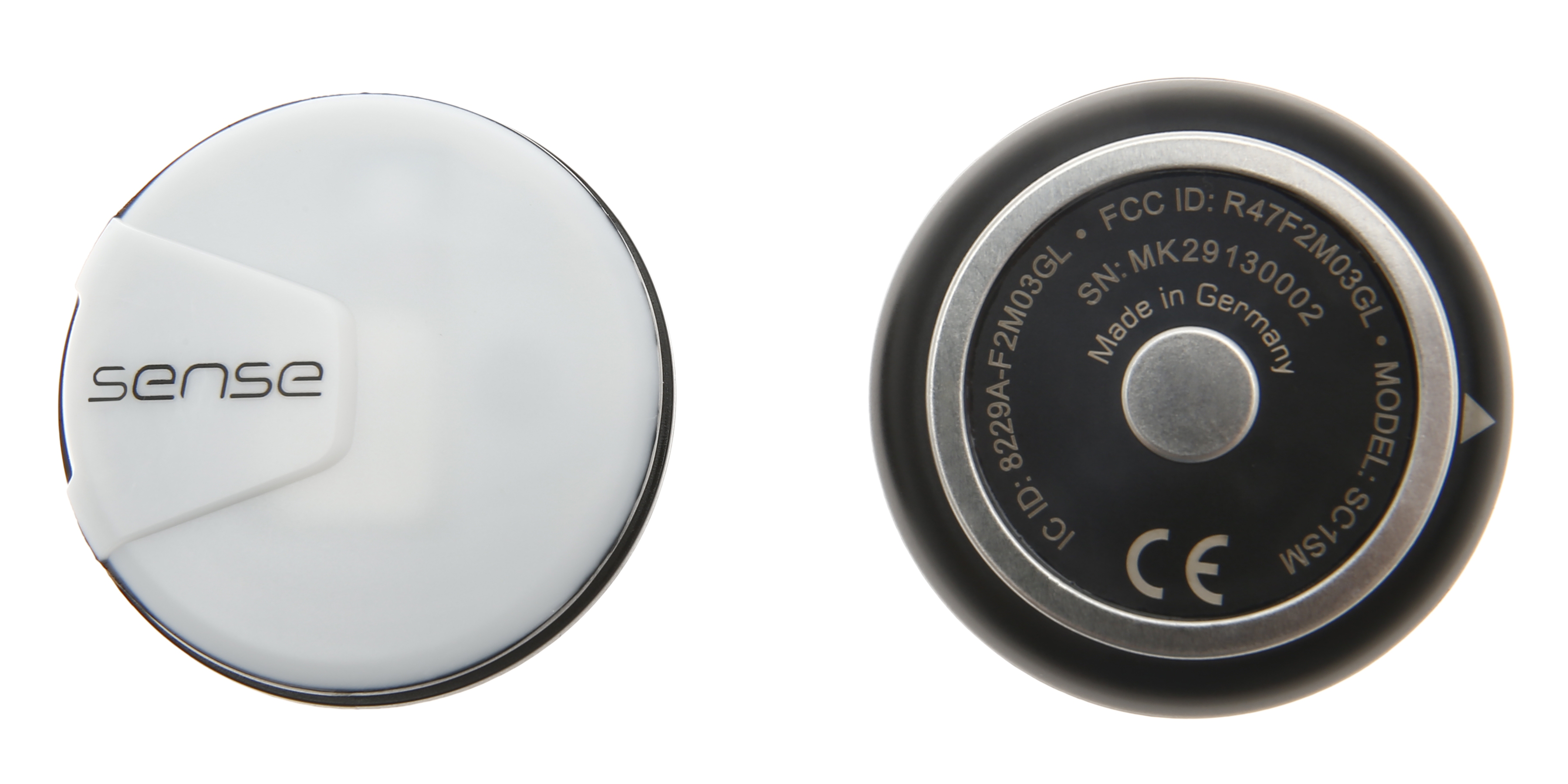
Figure 3: Cooperative sensors included in the smart vest for monitoring ECG.

This smart vest which was originally developed for athletes also monitors the following biomedical signals: heart rate, transthoracic impedance, respiration rate, skin temperature, activity class (resting, walking, running), and posture (lying, standing/sitting). A quality index is associated with each signal so that the reliability of the measurements can be easily assessed. However, these additional signals and the quality indices were not used in the present study. Figure 4 shows the smart vest during the validation protocol.

Figure 4: Smart vest during the validation protocol.

Another important feature of the smart vest consists in its capability to store all the recorded signals locally as well as synchronize them in the cloud. This is achieved by means of an accompanying gateway that acts as a relay for the streamed data. The gateway is robust to poor network connectivity and uploads the newly available data to the cloud as it is being streamed while an active connection is available. In our case, the gateway is composed of a simple Raspberry Pi that connects to the smart vest via Bluetooth. The biomedical data is then collected, stored locally in a compact format and relayed via telemetry messages simultaneously to all the clients connected to this gateway as well as a private cloud. The messaging protocol chosen for this application is MQTT (Message Queuing Telemetry Transport). This protocol, which uses the publish/subscribe paradigm, is one of the most widely employed telemetry protocols in IoT and real-time streaming. Once the ECG signal is in the cloud, we can leverage the powerful computing capabilities and detect heart arrhythmias with our neural network.

The ECG signals recorded with the smart vest device were pre-processed similarly to the data from the challenge of Computing in Cardiology 2017. First, the same band-pass filter between 0.5 and 40 Hz was used to remove the baseline and high-frequency noise. Then, the signals were resampled at 200 Hz. Finally, we scaled each signal with its standard deviation. Indeed, we could not use the scaling factor computed on the training set as the two types of ECG signals did not have the same range of values.

After pre-processing the ECG signals, we extracted sliding windows of 512 samples with 50% overlap. We used groups of 25 such windows as input to the neural network. We selected this specific number of windows as it corresponds to segments of approximately 33 seconds which is close to the median length of the signals used for training and testing the model. Applying the neural network resulted in a rhythm prediction for each group of 25 windows.

3 RESULTS

We evaluated three configurations. The first one used the architecture described in Table 2 except that it included only 6 convolutional layers. In addition, all data augmentation strategies were applied during training except resampling. The second configuration used the full architecture with 7 convolutional layers but again without resampling. Finally, the last configuration was identical to the second one but with resampling for further data augmentation. Figure 5 shows the evolution of the cross-entropy loss and the accuracy during training for these three network configurations. An additional convolutional layer helped to increase the accuracy and reduce the loss. Resampling the signals also slightly improved performance. Despite our efforts, we could not completely eliminate over-fitting as shown by the performance gap between training and test sets. Indeed, additional regularization only decreased the performance of the network. However, it is worth mentioning that resampling helped to reduce over-fitting. The neural network with the third configuration reached an accuracy of 87.37% on the test set after 47 epochs. At the same epoch, the accuracy on the training set was 90.90%.

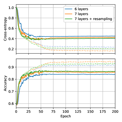
Figure 5: Cross-entropy loss (top) and accuracy (bottom) evaluated during training for a network with 6 convolutional layers without resampling (blue), a network with 7 convolutional layers without resampling (orange), and a network with 7 convolutional layers with resampling (green). Dashed lines denote results obtained on the training set and solid lines results obtained on the test set.

After selecting the best neural network, we evaluated it without zero-padding by selecting a batch size of 1. In this case, the accuracy was 92.64% on the training set and 87.50% on the test set. Sensitivity, specificity, and $F_{1}$ score values are reported in Table 3 for all classes. Unsurprisingly, the best $F_{1}$ score was obtained for the class with the most samples (normal rhythm) and the worst one for the class with the least samples (noise). Interestingly, the specificity for atrial fibrillation was relatively high at 0.9784 while the sensitivity was lower at 0.8382. Thus, the number of false positive is more larger than the number of false negative which is an important property of the model. Indeed, it missed only a few atrial fibrillation cases while false detections can always be disproved with additional analyses such as a full 12-lead ECG. Furthermore, when evaluated in terms of the score used during the challenge of Computing in Cardiology 2017 (1), the neural network yielded 0.9156 and 0.8495 on the training and test sets. This is similar to the best score obtained by the winners of the challenge. However, we could only evaluate our neural network on 1528 ECG signals from the original training set since the official test set was not made public yet. Therefore, it is difficult to compare the performance of our approach with the winning entries.

Table 3: Performance metrics for the best neural network.

Class	Metric	Training set	Test set
Normal rhythm	Sensitivity	0.9707	0.9263
	Specificity	0.8955	0.8853
	$F_{1}$ score	0.9509	0.9243
Atrial fibrillation	Sensitivity	0.9084	0.8382
	Specificity	0.9942	0.9784
	$F_{1}$ score	0.9232	0.8143
Other rhythm	Sensitivity	0.8380	0.7921
	Specificity	0.9675	0.9352
	$F_{1}$ score	0.8728	0.8099
Noise	Sensitivity	0.9345	0.7600
	Specificity	0.9972	0.9871
	$F_{1}$ score	0.9264	0.7103

After training and evaluation on the dataset of the challenge of Computing in Cardiology 2017, we applied the neural network to a few ECG signals recorded with the smart vest. We also extracted the times between consecutive R-waves from the ECG signals (a.k.a. RR intervals) to facilitate visualization of the heart rate. An example is shown in Figure 6. In this case, the subject had a normal sinus rhythm with two successive premature ventricular contractions characterized a very short RR interval followed by a long recovery RR interval. These premature contractions are clearly identifiable especially compared to the stable RR intervals of a normal rhythm. The neural network classified the this ECG segment as normal rhythm except for the groups of windows including the premature contractions which are classified as other rhythm.

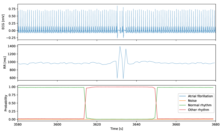
Figure 6: Cardiac rhythm classification from an ECG signal recorded with the smart vest. The ECG signal (top) includes two premature ventricular contractions which are visible in the RR intervals (middle). The neural network correctly identifies this segment of the signal as reflected by the class probabilities (bottom).

Another example of classification is shown in Figure 7. In this case, no ECG signal was collected during a few minutes due to poor skin-electrode contact caused by motion. The neural network identified this segment without signal as noise. Furthermore, two segments preceding signal loss were classified as normal rhythm and other rhythm. The RR intervals were stable in the first segment and there were a few premature ventricular contractions in the second one. After the ECG signal was recovered, the RR intervals varied widely and the neural network classified the data as other rhythm.

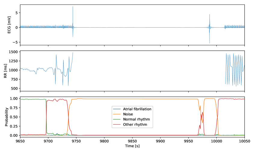
Figure 7: Cardiac rhythm classification from an ECG signal recorded with the smart vest. The ECG signal (top) includes a segment with no R waves due to poor skin-electrode contact. Consequently, the RR intervals (middle) could not be extracted. The class probabilities (bottom) computed by the neural network are valid as the segment is labeled as noise.

4 DISCUSSION

The neural network architecture we developed achieved a classification performance similar to the winners of the challenge of Computing in Cardiology 2017. Although we could not evaluate our approach on the same data since the true test set was not released yet, the results are promising. In particular, the specificity for atrial fibrillation shows that only a limited number cases are not detected. We could take into account signals of different lengths by combining convolutional and recurrent layers. Indeed, the convolutional layers extract features relevant for arrhythmia classification from sliding windows of raw ECG signal. With this approach, there is no need to pre-process the data to extract spectrogram or wavelet transform for instance. Furthermore, no feature engineering is required as the neural network learns during the training phase to extract high-level features useful for classification. The only pre-processing we used is band-pass filtering as well as scaling to accelerate training. We also used strategies for data augmentation to reduce over-fitting and improve the generalization performance of the network. In particular, randomly flipping the sign of ECG signals forced the neural network to learn to take into account both regular and inverted waveforms. Without this simple strategy, we would have needed to develop a robust method to detect signals that had to be rectified.

In addition, we have shown that it is possible to apply a neural network trained on a generic dataset to ECG signals recorded by the smart vest with minimal changes. Indeed, there was no need to adapt the network architecture. The method to standardize the ECG signals was the only element that required a modification. Of course, if the two measurement systems, the AliveCor device and the smart vest, did not record the same ECG lead, additional changes would be needed. However, it is difficult to determine the extend of these changes without evaluating the neural network on a dataset of ECG signals from another lead.

Taken together, these results demonstrate that our system could be used to monitor the cardiac activity of a subject for detecting abnormal rhythms over long periods of time. Indeed, the smart vest is more comfortable to wear than a traditional Holter and it can still collect high quality ECG signals since it was initially developed for athletes. After transmitting the data to the cloud, our neural network can quickly classify abnormal rhythms. While the accuracy of our system is not perfect, it can still help to reduce the time spent reviewing ECG by selecting segments with potential abnormalities that require additional attention. These segments can then be analyzed by a trained specialist. If needed, a full 12-lead ECG can be performed to refine or confirm the diagnosis.

5 CONCLUSION

We presented a system composed of a smart vest to record a single lead ECG signal and a neural network for detection and classification of heart arrhythmias. We plan to aggregate several databases of ECG signals with rhythm annotations to extend the types of arrhythmias that our algorithm can detect and improve its accuracy. We will also investigate whether adding skip connections in our network architecture further improves classification performance.

REFERENCES

- Camm et al., 2010 Camm, A. J. et al. (2010). Guidelines for the management of atrial fibrillation. European Heart Journal, 31(19):2369–2429.
- Chollet et al., 2015 Chollet, F. et al. (2015). Keras. https://keras.io.
- Clifford et al., 2017 Clifford, G. D., Liu, C., Moody, B., Lehman, L.-w. H., Silva, I., Li, Q., Johnson, A., and Mark, R. G. (2017). AF classification from a short single lead ECG recording: The PhysioNet/Computing in Cardiology Challenge 2017. Proceedings of Computing in Cardiology, 44:1.
- Datta et al., 2017 Datta, S., Puri, C., Mukherjee, A., Banerjee, R., Choudhury, A. D., Singh, R., Ukil, A., Bandyopadhyay, S., Pal, A., and Khandelwal, S. (2017). Identifying normal, AF and other abnormal ECG rhythms using a cascaded binary classifier. In 2017 Computing in Cardiology (CinC), pages 1–4.
- De Chazal et al., 2004 De Chazal, P., O’Dwyer, M., and Reilly, R. B. (2004). Automatic classification of heartbeats using ECG morphology and heartbeat interval features. IEEE Transactions on Biomedical Engineering, 51(7):1196–1206.
- Frick et al., 2001 Frick, M., Frykman, V., Jensen-Urstad, M., and Östergren, J. (2001). Factors predicting success rate and recurrence of atrial fibrillation after first electrical cardioversion in patients with persistent atrial fibrillation. Clinical Cardiology, 24(3):238–244.
- Gal and Ghahramani, 2016 Gal, Y. and Ghahramani, Z. (2016). A theoretically grounded application of dropout in recurrent neural networks. In Advances in neural information processing systems, pages 1019–1027.
- Hahnloser et al., 2000 Hahnloser, R. H., Sarpeshkar, R., Mahowald, M. A., Douglas, R. J., and Seung, H. S. (2000). Digital selection and analogue amplification coexist in a cortex-inspired silicon circuit. Nature, 405(6789):947.
- Hochreiter and Schmidhuber, 1997 Hochreiter, S. and Schmidhuber, J. (1997). Long short-term memory. Neural Computation, 9(8):1735–1780.
- Hong et al., 2017 Hong, S., Wu, M., Zhou, Y., Wang, Q., Shang, J., Li, H., and Xie, J. (2017). ENCASE: An ENsemble ClASsifiEr for ECG classification using expert features and deep neural networks. In 2017 Computing in Cardiology (CinC), pages 1–4.
- January et al., 2014 January, C. T., Wann, L. S., Alpert, J. S., Calkins, H., Cigarroa, J. E., Cleveland, J. C., Conti, J. B., Ellinor, P. T., Ezekowitz, M. D., Field, M. E., Murray, K. T., Sacco, R. L., Stevenson, W. G., Tchou, P. J., Tracy, C. M., and Yancy, C. W. (2014). 2014 AHA/ACC/HRS guideline for the management of patients with atrial fibrillation: a report of the American College of Cardiology/American Heart Association task force on practice guidelines and the Heart Rhythm Society. Journal of the American College of Cardiology, 64(21):e1–e76.
- Kannel et al., 1998 Kannel, W. B., Wolf, P. A., Benjamin, E. J., and Levy, D. (1998). Prevalence, incidence, prognosis, and predisposing conditions for atrial fibrillation: population-based estimates. The American journal of cardiology, 82(7):2N–9N.
- Kingma and Ba, 2014 Kingma, D. P. and Ba, J. (2014). Adam: A method for stochastic optimization. arXiv preprint arXiv:1412.6980.
- Krizhevsky et al., 2012 Krizhevsky, A., Sutskever, I., and Hinton, G. E. (2012). ImageNet classification with deep convolutional neural networks. In Advances in Neural Information Processing Systems 25, pages 1097–1105.
- LeCun et al., 2012 LeCun, Y. A., Bottou, L., Orr, G. B., and Müller, K.-R. (2012). Efficient backprop. In Neural networks: Tricks of the trade, pages 9–48. Springer.
- Nattel et al., 2008 Nattel, S., Burstein, B., and Dobrev, D. (2008). Atrial remodeling and atrial fibrillation: mechanisms and implications. Circulation: Arrhythmia and Electrophysiology, 1(1):62–73.
- Owis et al., 2002 Owis, M. I., Abou-Zied, A. H., Youssef, A.-B., and Kadah, Y. M. (2002). Study of features based on nonlinear dynamical modeling in ECG arrhythmia detection and classification. IEEE Transactions on Biomedical Engineering, 49(7):733–736.
- Rajpurkar et al., 2017 Rajpurkar, P., Hannun, A. Y., Haghpanahi, M., Bourn, C., and Ng, A. Y. (2017). Cardiologist-level arrhythmia detection with convolutional neural networks. arXiv preprint arXiv:1707.01836.
- Srivastava et al., 2014 Srivastava, N., Hinton, G., Krizhevsky, A., Sutskever, I., and Salakhutdinov, R. (2014). Dropout: a simple way to prevent neural networks from overfitting. The Journal of Machine Learning Research, 15(1):1929–1958.
- Teijeiro et al., 2017 Teijeiro, T., García, C. A., Castro, D., and Félix, P. (2017). Arrhythmia classification from the abductive interpretation of short single-lead ECG records. In 2017 Computing in Cardiology (CinC), pages 1–4.
- Wang et al., 2003 Wang, T. J., Larson, M. G., Levy, D., Vasan, R. S., Leip, E. P., Wolf, P. A., D’Agostino, R. B., Murabito, J. M., Kannel, W. B., and Benjamin, E. J. (2003). Temporal relations of atrial fibrillation and congestive heart failure and their joint influence on mortality: the Framingham heart study. Circulation, 107(23):2920–2925.
- Xia et al., 2018 Xia, Y., Wulan, N., Wang, K., and Zhang, H. (2018). Detecting atrial fibrillation by deep convolutional neural networks. Computers in Biology and Medicine, 93:84–92.
- Xiong et al., 2017 Xiong, Z., Stiles, M. K., and Zhao, J. (2017). Robust ECG signal classification for detection of atrial fibrillation using a novel neural network. In 2017 Computing in Cardiology (CinC), pages 1–4.
- Zabihi et al., 2017 Zabihi, M., Rad, A. B., Katsaggelos, A. K., Kiranyaz, S., Narkilahti, S., and Gabbouj, M. (2017). Detection of atrial fibrillation in ECG hand-held devices using a random forest classifier. In 2017 Computing in Cardiology (CinC), pages 1–4.
- Zihlmann et al., 2017 Zihlmann, M., Perekrestenko, D., and Tschannen, M. (2017). Convolutional recurrent neural networks for electrocardiogram classification. In 2017 Computing in Cardiology (CinC), pages 1–4.