Semiclassical Vibrational Spectroscopy with Hessian Databases

Abstract

We report on a new approach to ease the computational overhead of ab initio “on-the-fly” semiclassical dynamics simulations for vibrational spectroscopy. The well known bottleneck of such computations lies in the necessity to estimate the Hessian matrix for propagating the semiclassical pre-exponential factor at each step along the dynamics. The procedure proposed here is based on the creation of a dynamical database of Hessians and associated molecular geometries able to speed up calculations while preserving the accuracy of results at a satisfactory level. This new approach can be interfaced to both analytical potential energy surfaces and on-the-fly dynamics, allowing one to study even large systems previously not achievable. We present results obtained for semiclassical vibrational power spectra of methane, glycine, and N-acetyl-L-phenylalaninyl-L-methionine-amide, a molecule of biological interest made of 46 atoms.

I Introduction

Several computational methods for calculating quantum molecular vibrational spectra have been established. To name some popular ones, we recall the vibrational self-consistent field and virtual space configuration interaction (VSCF/VCI) method,(Bowman, Carter, and Huang, 2003; Bowman, Carrington, and Meyer, 2008; Huang, Habershon, and Bowman, 2008; Mancini and Bowman, 2014) the multi-configuration time dependent Hartree (MCTDH) approach,(Meyer, Manthe, and Cederbaum, 1990; Meyer and Worth, 2003; Vendrell, Gatti, and Meyer, 2007; Picconi, Cina, and Burghardt, 2019a, b) the use of contracted basis functions with an eigensolver,(Cullum and Willoughby, 2015; Davidson, 1975) collocation methods,(Manzhos and Carrington, 2016; Avila and CarringtonJr., 2017) and second-order vibrational perturbation theory (VPT2).(Barone, 2005) Despite the advance these methods provide in dealing with the exponential scaling of quantum approaches with the number of vibrational degrees of freedom, the investigation of large molecules or complex supra-molecular systems remains quite challenging. In this case classical simulations or ad-hoc scaling of harmonic estimates are the approaches commonly employed in spite of the drawback of totally neglecting or not properly describing quantum effects (such as zero-point energies, quantum couplings, and overtones). This aspect has been recently confirmed by a semiclassical (SC) investigation,(Gabas et al., 2018) which has explained experimental findings due to quantum effects, in contrast to previous non conclusive theoretical attempts.(Masson, Williams, and Rizzo, 2015; Oh et al., 2005) Furthermore, recent SC techniques which are capable of accurately calculating the intensities of vibrational spectral transitions have demonstrated that the widely employed double harmonic approximation often provides only a rough estimate, which has to be corrected by incorporating quantum couplings and anharmonicities.(Micciarelli et al., 2018, 2019)

Semiclassical dynamics is indeed gaining more and more attention due to some of its peculiar features, which include the possibility of accounting for quantum effects in an accurate way starting from short-time classical trajectories,(Miller, 1974; Heller, 1981; Herman and Kluk, 1984; Miller, 1991; Kay, 1994a; Walton and Manolopoulos, 1995; Elran and Kay, 1999; Grossmann, 1999; Shalashilin and Child, 2001; Miller, 2005; Kay, 2005; Liu and Miller, 2007; Ceotto et al., 2009a; Ceotto, Dell‘ Angelo, and Tantardini, 2010; Ceotto, Tantardini, and Aspuru-Guzik, 2011; Tamascelli et al., 2014; Wehrle, Oberli, and Vaníček, 2015; Buchholz, Grossmann, and Ceotto, 2018; Ma et al., 2018; Conte and Ceotto, pted; Church, Antipov, and Ananth, 2017; Bonella, Montemayor, and Coker, 2005; Tao and Miller, 2011, 2012; Tao, 2014, 2013) the advantage of not being limited to a single-well picture,(Conte, Aspuru-Guzik, and Ceotto, 2013; Gabas, Conte, and Ceotto, 2017; Di Liberto, Conte, and Ceotto, 2018a) and the possibility of adopting an ab initio “on-the-fly” approach.(Ceotto et al., 2009b; Tatchen and Pollak, 2009; Ceotto et al., 2011; Wehrle, Sulc, and Vanicek, 2014; Patoz, Begusic, and Vanicek, 2018; Gabas, Conte, and Ceotto, 2017) These characteristics make the range of applicability of semiclassical spectroscopy enormously vast, ranging from small molecules, for which very precise analytical potential energy surfaces (PES) can be constructed, to larger molecules or even supra-molecular systems whose dynamics can be integrated “on-the-fly” from ab initio calculations. Clearly, a very different computational effort is required depending on whether calls to the potential are analytical or ask for ab initio electronic structure calculations as in the case of “on-the-fly” simulations.(Pratihar et al., 2017; Marx and Hutter, 2009; Marx and Parrinello, 1996; Galimberti et al., 2017; Gaigeot, 2010) In SC dynamics this difference translates mainly into the very different number of trajectories on which SC calculations are based. In fact, when working with an analytical PES and exploiting time-average (TA) filtering techniques, a proper Monte Carlo convergence in the evaluation of the semiclassical phase-space integration can be reached.(Kaledin and Miller, 2003a, b) A tailored approach, known as Multiple Coherent Semiclassical Initial Value Representation (MC SCIVR), must be employed instead when adopting “on-the-fly” dynamics, so that even a single tailored trajectory allows one to regain the main spectral features.(Ceotto et al., 2009a; Gabas, Conte, and Ceotto, 2017)

Application of standard SC techniques is hampered by a few well-known drawbacks. One is the so-called “curse of dimensionality” which concerns the impossibility of obtaining a resolved spectroscopic signal when the dimensionality of the system becomes too large. Another one is related to the chaotic behavior of classical dynamics. Chaotic trajectories make numerical integration of the monodromy matrix elements (needed to evaluate the SC frozen Gaussian propagator) inaccurate because of finite machine precision. The consequence is that, if the contribution of these trajectories is neither discarded nor reshaped, the entire calculation may be spoiled. However, even in the case of non-chaotic trajectories, propagation of the monodromy matrix elements represents a computational bottleneck due to the necessity to evaluate the Hessian matrix (matrix of second derivatives of the potential with respect to the nuclear coordinates) at each step along the dynamics.

Recent advances in the semiclassical field have permitted researchers to make progress on these issues and further research is still being carried out. For instance, a “divide-and-conquer” strategy (DC SCIVR) has been employed to extend semiclassical spectroscopy to systems as large as fullerene;(Ceotto, Di Liberto, and Conte, 2017; Di Liberto, Conte, and Ceotto, 2018b, a) appropriate approximations have been introduced to deal with chaotic trajectories;(Kay, 1994b; Gelabert et al., 2000; Di Liberto and Ceotto, 2016; Gabas, Conte, and Ceotto, 2017) and a compact finite-difference (CFD) approximation to the Hessian has been able to reduce the number of Hessian calculations required.(Wu et al., 2010; Zhuang et al., 2012; Ahmadian et al., 2017) In particular, CFD-Bofill schemes permit one to preserve the accuracy in the propagation of monodromy matrix elements quite well and, using them, accurate semiclassical spectra have been obtained for several small molecules including an “on-the-fly” application to CO₂.(Ceotto, Zhuang, and Hase, 2013)

So far this introduction has been focused on SC frozen Gaussian propagators, which were employed in the numerical applications presented in this paper. However, Hessian calculations are ubiquitous in semiclassical dynamics and, in fact, they are required also by another variety of SC propagators, known as thawed Gaussian propagators.(Heller, 1975; Baranger et al., 2001; Pollak and Miret-Artés, 2004; Grossmann, 2006; Conte and Pollak, 2010) The main difference between the two families is that in a frozen Gaussian the width of the Gaussians is a constant in time, while in a thawed Gaussian the width evolves in time. Furthermore, SC thawed Gaussian calculations are based on single-trajectory dynamics and are known to be less accurate than their frozen Gaussian counterparts even in the case of MC SCIVR single trajectory simulations. Interpolation schemes have been developed for thawed Gaussian propagators,(Wehrle, Sulc, and Vanicek, 2014; Buchholz, Grossmann, and Ceotto, 2016, 2017; Buchholz et al., 2012; Begusic, Roulet, and Vanicek, 2018; Patoz, Begusic, and Vanicek, 2018) and, at the time of writing, an approach based on a single, initial Hessian evaluation has just been proposed and applied to SC thawed Gaussian vibro-electronic (vibronic) calculations.(Begusic, Cordova, and Vanicek, 2019)

The main goals of this paper are the introduction of a new strategy to slash the computational overhead associated with Hessian matrix calculations and its application to precise semiclassical frozen Gaussian vibrational spectroscopy of polyatomic molecular systems. The approach is based on the dynamical construction of a database of Hessian matrices dependent on the molecular geometry visited along the dynamics. It is not as computationally inexpensive as the thawed Gaussian single Hessian scheme, but more accurate. We show that this Hessian approximation is accurate, and able to extend the range of applicability of “on-the-fly” SC vibrational spectroscopy to larger chemical species. The paper introduces the theoretical details of the new approach in Section II. Section III is devoted to applications to methane, glycine and N-acetyl-L-phenylalaninyl-L-methionine-amide. Finally, in Section IV, a summary and some conclusions are reported.

II Theoretical and Computational Details

The semiclassical calculation of vibrational power spectra of molecular species is a long established technique, which does not suffer from zero point energy (ZPE) leakage(Buchholz et al., 2018) and has recently evolved into a very powerful computational tool able to deal with systems involving dozens of degrees of freedom. In this Section we introduce the SC theoretical methodology on which our results are based, and then focus on the description of the new database strategy.

In a pivotal paper(Kaledin and Miller, 2003a) Kaledin and Miller demonstrated that by time averaging the Herman-Kluk semiclassical propagator, it is possible to work out a computationally advantageous expression for the power spectrum of a survival amplitude evolved according to a vibrational Hamiltonian. Their starting point, the Herman-Kluk (HK) propagator, provides a semiclassical approximation to the exact quantum propagator. In particular, for an $N_{vib}$-dimensional system, the survival amplitude of a generic reference state $|\chi\rangle$ can be written as

$$\left\langle\chi\left|e^{-i\hat{H}t/\hbar}\right|\chi\right\rangle_{HK}=\left(\frac{1}{2\pi\hbar}\right)^{N_{vib}}\iintop d\mathbf{p}_{0}d\mathbf{q}_{0}C_{t}\left(\mathbf{p}_{0},\mathbf{q}_{0}\right)e^{\frac{i}{\hbar}S_{t}\left(\mathbf{p}_{0},\mathbf{q}_{0}\right)}\left\langle\chi\right.\left|\mathbf{p}_{t},\mathbf{q}_{t}\left\rangle\right\langle\mathbf{p}_{0},\mathbf{q}_{0}\right|\left.\chi\right\rangle.$$ (1)

The Monte Carlo integration needed to evaluate the rhs of Eq. (1) is performed by generating a set of phase space points (p₀, q₀) according to the distribution function defined by the overlap $\langle\mathbf{p}_{0},\mathbf{q}_{0}|\chi\rangle$. $|{\bf p},{\bf q}\rangle$ indicates a coherent state, which has a Gaussian representation in both position and momentum space. Specifically,

$$\left\langle\mathbf{x}|\mathbf{p},\mathbf{q}\right\rangle=\left(\frac{\text{det}(\boldsymbol{\Gamma})}{\pi^{N_{vib}}}\right)^{1/4}e^{-\frac{1}{2}\left(\mathbf{x}-\mathbf{q}\right)^{T}\Gamma\left(\mathbf{x}-\mathbf{q}\right)+i\mathbf{p}^{T}\left(\mathbf{x}-\mathbf{q}\right)/\hbar},$$ (2)

where $\boldsymbol{\Gamma}$ is the N_vib × N_vib coherent state width matrix that is generally chosen to be diagonal with elements equal to the harmonic frequencies of vibrations. The select phase space points (p₀, q₀) serve as starting conditions for classical dynamics runs that permit one to evaluate the whole integrand. In fact, at every time t along the dynamics, the coherent state overlap $\langle\chi|\mathbf{p}_{t},\mathbf{q}_{t}\rangle$ is readily estimated; S_t(p₀, q₀) is the instantaneous classical action, and C_t(p₀, q₀) is the Herman-Kluk pre-exponential factor defined as

$$C_{t}\left(\mathbf{p}_{0},\mathbf{q}_{0}\right)=\sqrt{\left|\frac{1}{2}\left(\frac{\partial\mathbf{q}_{t}}{\partial\mathbf{q}_{0}}+\boldsymbol{\Gamma}^{-1}\frac{\partial\mathbf{p}_{t}}{\partial\mathbf{p}_{0}}\boldsymbol{\Gamma}-i\hbar\frac{\partial\mathbf{q}_{t}}{\partial\mathbf{p}_{0}}\boldsymbol{\Gamma}+\frac{i\boldsymbol{\Gamma}^{-1}}{\hbar}\frac{\partial\mathbf{p}_{t}}{\partial\mathbf{q}_{0}}\right)\right|}.$$ (3)

The Fourier transform of Equation (1) yields the SC power spectrum (i.e. the spectral density) associated to the vibrational Hamiltonian $\hat{H}$

$$I(E)_{HK}=\dfrac{Re}{\pi\hbar}\int_{0}^{+\infty}dt\;e^{iEt/\hbar}\;\left\langle\chi\left|e^{-i\hat{H}t/\hbar}\right|\chi\right\rangle_{HK}.$$ (4)

The SC estimates of the molecular eigenenergies of vibration correspond to the energy values at which the peaks in the power spectrum are localized. The ground state energy, i.e. the zero point energy, is commonly shifted to zero and, in this case, the peaks in the power spectrum are centered at the quantum (semiclassical) transition frequencies of fundamentals and overtones. Unfortunately, convergence of the phase space Monte Carlo integration for the Herman Kluk propagator is too slow for application to sizeable molecular systems due to the oscillatory nature of its integrand. This issue is overcome by Kaledin and Miller’s time average filter, which leads to a more efficient formula for the spectral density known as the time averaged semiclassical initial value representation (TA SCIVR)

$$I(E)_{TASCIVR}=\left(\frac{1}{2\pi\hbar}\right)^{N_{vib}}\iintop d\mathbf{p}_{0}d\mathbf{q}_{0}\frac{1}{2\pi\hbar T}\left|\intop_{0}^{T}e^{\frac{i}{\hbar}\left[S_{t}\left(\mathbf{p}_{0},\mathbf{q}_{0}\right)+Et+\phi_{t}\left(\mathbf{p}_{0},\mathbf{q}_{0}\right)\right]}\langle\chi|\mathbf{p}_{t},\mathbf{q}_{t}\rangle dt\right|^{2}.$$ (5)

In Eq.(5) $\phi_{t}\left(\mathbf{p}_{0},\mathbf{q}_{0}\right)$ is the phase of the original complex-valued Herman-Kluk pre-exponential factor introduced owing to the so-called “separable” approximation,(Kaledin and Miller, 2003a) and T is the total time of the dynamics. The key advantage of Eq. (5) is that the integrand is positive definite and this facilitates the numerical convergence of the integration. The derivation of Eq. (5) is discussed extensively in Ref. 59, and the interested reader can find all the details therein.

For the purposes of this work it is important to point out that Eq. (5) is the basic working formula for our spectral simulations. It has been applied previously to several molecules and further developed to interface the TA-SCIVR formalism to “on-the-fly” dynamics for application to much larger molecular systems. Specifically, on-the-fly simulations must rely on a limited number of trajectories to be computationally affordable. This is achieved by adopting for each vibrational state a few tailored trajectories (i.e. SC propagators) and reference states $|\chi\rangle$, a technique known as multiple coherent semiclassical initial value representation (MC SCIVR). The trajectories are run at an energy corresponding to the harmonic estimate for the generic k-th state to investigate, while the corresponding reference state is chosen as

$$\left|\chi^{(k)}\right\rangle=\prod_{i=1}^{N_{vib}}\sum_{j=1}^{N_{\alpha}}\boldsymbol{\varepsilon}_{ij}^{(k)}\left|p_{eq,i}^{(k)},q_{eq,i}^{(k)}\right\rangle.$$ (6)

The coherent states in Eq.(6) are centered at specific positions and momenta $({\bf p}_{eq}^{(k)},{\bf q}_{eq}^{(k)})$, which determine the initial conditions and the energy of the classical trajectories needed by the semiclassical simulation. $\text{\text{N}}_{\alpha}$ accounts for the possible duplication of coherent states, which are linearly combined through the array of integers ($\boldsymbol{\varepsilon}$), to enforce parity and molecular symmetries. Parity symmetry allows to enhance specific peaks in the power spectrum (i.e. the ground state, specific fundamental transitions, or overtones) and it is obtained by inverting the sign of the momentum in the duplicate coherent state. Molecular symmetry (detection of peaks corresponding to vibrations belonging to a specific irreducible representation of the symmetry group of the molecule) is introduced by inverting the sign of the (equilibrium) positions in the duplicate coherent state.(Kaledin and Miller, 2003b; Ceotto et al., 2009a) The greatest novelty of the MC SCIVR procedure is that accurate results can be obtained by running just one tailored trajectory per state with the effect of alleviating the computational cost substantially.

Another problem related to Eq. (5) is that the coherent state overlap $\langle\chi|\mathbf{p}_{t},\mathbf{q}_{t}\rangle$ is more and more likely to give a negligible contribution as N_vib increases, so that a spectrally resolved Fourier signal is harder and harder to collect. A very recent advance able to overcome this problem is the divide-and-conquer semiclassical initial value representation (DC SCIVR), which is based on performing semiclassical calculations in lower dimensional subspaces. The dynamics is still performed in full dimensionality permitting one to recover at least partially the interaction between different subspaces, and Eq. (5) remains the working formula. The several quantities appearing in the integrand of Eq. (5) are readily projected onto the subspaces with the exception of the action, which requires a redefinition of the projected potential energy due to its non-separability in general. For an M-dimensional subspace

$$\tilde{I}(E)_{DCSCIVR}=\left(\frac{1}{2\pi\hbar}\right)^{M}\iintop d\tilde{\mathbf{p}}_{0}d\tilde{\mathbf{q}}_{0}\frac{1}{2\pi\hbar T}\left|\intop_{0}^{T}e^{\frac{i}{\hbar}\left[\tilde{S}_{t}\left(\tilde{\mathbf{p}}_{0},\tilde{\mathbf{q}}_{0}\right)+Et+\tilde{\phi}_{t}\left(\tilde{\mathbf{p}}_{0},\tilde{\mathbf{q}}_{0}\right)\right]}\langle\tilde{\chi}|\tilde{\mathbf{p}}_{t},\tilde{\mathbf{q}}_{t}\rangle dt\right|^{2}.$$ (7)

$$\tilde{S}_{t}(\tilde{\mathbf{p}}_{0},\tilde{\mathbf{q}}_{0})=\int_{0}^{t}dt^{\prime}\,(\tilde{T}(t^{\prime})-\tilde{V}(t^{\prime})),$$

$$\tilde{V}(t^{\prime})=V(\tilde{q}_{M}(t^{\prime});q_{N_{vib}-M}^{eq})+\lambda(t^{\prime});$$

$$\lambda(t)=V(\tilde{q}_{M}(t);q_{N_{vib}-M}(t))-[V(\tilde{q}_{M}^{eq};q_{N_{vib}-M}(t)+V(\tilde{q}_{M}(t);q_{N_{vib}-M}^{eq})];$$

$$\tilde{V}(t^{\prime})=V(\tilde{q}_{M}(t^{\prime});q_{N_{vib}-M}(t^{\prime}))-V(\tilde{q}_{M}^{eq};q_{N_{vib}-M}(t^{\prime})).$$ (8)

Projected quantities in Eqs. (7) and (8) are indicated by tildes. Upon parametrization of the degrees of freedom external to the M-dimensional subspace and correction by means of the external time-dependent field $\lambda(t),$ the projected potential is obtained as a difference between the instantaneous potential and the potential at the corresponding unrelaxed subspace minimum. Combination of the multiple coherent and divide-and-conquer techniques, named MC-DC SCIVR is feasible and effective. A complete treatment of DC SCIVR can be found in Refs.61; 62, where appropriate strategies for determining the best suited subspaces have been illustrated and discussed.

A final issue concerning Eq. (5) is that evolution of the phase $\phi_{t}\left(\mathbf{p}_{0},\mathbf{q}_{0}\right)$, which bears key quantum effects, requires to calculate the Hessian matrix along the whole classical trajectory and the computational effort therefore increases rapidly with the number of degrees of freedom. This is the bottleneck of semiclassical calculations plaguing both full dimensional and DC-SCIVR approaches. To overcome the problem it is necessary to find a way to reduce the number of Hessian calculations while keeping a sufficient accuracy for vibrational frequencies. A first effort in this direction has been made by developing a compact finite-difference approximation.(Ceotto, Zhuang, and Hase, 2013) If the Hessian is calculated at the i-th step of the dynamics ($\mathcal{H}_{i}$), then the approximation estimates $\mathcal{H}_{j}$ (j=i+1,…,i+N-1) at the following N-1 steps according to the formula

$$\mathcal{\mathcal{H}}_{j}=\mathcal{H}_{j-1}+(1-\lambda)\dfrac{\boldsymbol{R}\boldsymbol{R}^{T}}{\boldsymbol{R}^{T}\Delta\boldsymbol{q}}+\lambda\left(\dfrac{\Delta\boldsymbol{q}\boldsymbol{R}^{T}+\boldsymbol{R}^{T}\Delta\boldsymbol{q}}{||\Delta\boldsymbol{q}||^{2}}-\dfrac{\boldsymbol{R}^{T}\Delta\boldsymbol{q}}{||\Delta\boldsymbol{q}||^{4}}\Delta\boldsymbol{q}\Delta\boldsymbol{q}^{T}\right),$$ (9)

where $\lambda$ is a parameter identifying different families of approximations according to its value; $\Delta$q = q_j - q_i, and R = 2(g_j - g_i - $\mathcal{H}$_i$\Delta$q) with g_i being the gradient at the i-th geometry. The simplest form of the approximation employs the value $\lambda$ = 1, and it is known as the Hessian Update (HU) Powell Symmetric Broyden scheme. A more refined choice of $\lambda$ leads to the HU Bofill approximation. Calculation of the Hessian matrix is performed only at intervals of N steps, while, according to Eq. (9), only the computationally cheaper gradient must be evaluated for all the other steps. These schemes have been shown to work well for small-to-medium size molecules.(Wu et al., 2010; Zhuang et al., 2012; Ceotto, Zhuang, and Hase, 2013)

In this work we introduce an alternative strategy to decrease the number of Hessian calculations. It is based on the dynamical creation of a database of Hessians (DBH) and related geometries, which can be exploited whenever the instantaneous molecular geometry is close enough to one of the $N_{db}$ records already present in the database. An estimate of the “distance” between two molecular configurations can be obtained either by evaluating the root mean square difference between vibrational normal mode coordinates in the two configurations,

$$\sigma\,({\bf q},{\bf q}_{db})=\sqrt{\dfrac{\sum_{l=1}^{N_{vib}}(q_{l}-q_{l,db})^{2}}{N_{vib}}},$$ (10)

where $q_{l}$ and $q_{l,db}$ are the values of the l-th normal mode for the instantaneous geometry and one included in the database respectively, or by estimating the absolute difference for each mode

$$\Theta{}_{l}\,({\bf q},{\bf q}_{db})=|q_{l}-q_{l,db}|,\quad l=1,\ldots,N_{vib}.$$ (11)

To determine whether the two configurations are enough close or not, an arbitrary threshold $\rho$ is introduced. It is straightforward to demonstrate that $\sigma\,({\bf q},{\bf q}_{db})<\rho$ is a weaker condition than having the $\Theta\,({\bf q},{\bf q}_{db})$ test passed for each mode, i.e. $\Theta_{l}\,({\bf q},{\bf q}_{db})<\rho\quad\forall l\in[1,N_{db}]$. For this reason we employ Eq. (11) to determine the set of suitable records in the database, while Eq.(10) is used to identify the closest among database candidates (${\bf q}_{db}^{closest}$) to the instantaneous geometry.

The search for the best match among the N_db records ${\bf q}$_db in the database for the instantaneous geometry ${\bf q}$ is another important aspect of the method since it may become computationally costly when the size of the database grows large. To accelerate the search, mode-1 components of geometries in the database are sorted in increasing order. The algorithm starts with calculation of $\Theta_{1}\,({\bf q},{\bf q}_{db})$ along the database and check of the $\Theta_{1}\,({\bf q},{\bf q}_{db})<\rho$ condition. Once the test is passed, the search based on the first normal mode is stopped as soon as $\Theta_{1}\,({\bf q},{\bf q}_{db})>\rho$. Then, the $\Theta_{l}\,({\bf q},{\bf q}_{db})<\rho$ condition is evaluated sequentially for the other normal modes only on the restricted set of records that have passed all previous $\Theta_{l^{\prime}}\,({\bf q},{\bf q}_{db})<\rho,\,l^{\prime}=1,\ldots,l-1$ tests.

If, after all N_vib modes have been examined, there are one or more configurations still left, then the Hessian associated with the geometry with the smallest $\sigma\,({\bf q},{\bf q}_{db})$ value, i.e. ${\bf q}_{db}^{closest}$, is selected to approximate the instantaneous Hessian in the SC simulation. Otherwise, a new Hessian calculation is performed and added to the database in the correct k-th position as determined by its ${\bf q}_{1,db}$ value. Figure 1 shows the flow chart for the method.

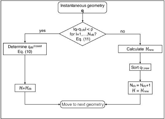
Figure 1: Flow chart for the DBH method.

Some preliminary tests on systems of increasing dimensionality have been undertaken to check on the performance of the approach depending on database size, threshold $\rho$, and system complexity. As a first test, we employed analytical water(Bowman, Wierzbicki, and Zuniga, 1988) and methane(Lee, Martin, and Taylor, 1995) potentials to construct three databases of different sizes by running different numbers of trajectories. Then, an additional trajectory was run to evaluate, at a specific value of $\rho$: i) the number of geometries for which a suitable match in the database was found; ii) the root mean square deviation ($\sigma_{Hess}$) of the elements of the associated Hessian in the database from those calculated at the trajectory instantaneous geometry. $\sigma$_Hess is defined as

$$\sigma_{Hess}=\sqrt{\dfrac{\sum_{m}^{N_{vib}}\sum_{n}^{N_{vib}}(\mathcal{\mathcal{H}}_{mn}-\mathcal{\mathcal{H}}_{mn,db})^{2}}{N_{vib}-1}},$$ (12)

where $\mathcal{\mathcal{H}}_{mn}$ is the (m,n) component of the Hessian matrix. A single test trajectory is representative of the general case of interest for SC simulations in which initial conditions are sampled around the equilibrium geometry.

Table 1 reports the results. Each trajectory was evolved in full dimensionality with a symplectic algorithm for a total of 2,500 steps, i.e. it is made of 2,500 geometries. The larger the database becomes, the easier it is to find a suitable record in it and the more accurate the Hessian database estimate.

Table 1: Comparison of different databases for H₂O and CH₄. The threshold parameter is $\rho$ = 1 for H₂O and $\rho$ = 10 for CH₄. N^db indicates the number of geometries constituting the database; N^mg is the number of geometries of the test trajectory for which a matching database entry is found; $\sigma_{Hess}$ is the root mean square deviation of the Hessian elements for the matched geometries, as defined in Eq. (12).

H2O			CH4
Ndb	Nmg	$\sigma_{Hess}$	Ndb	Nmg	$\sigma_{Hess}$
2500	295	9.4 10-6	2500	118	5.3 10-5
25000	2157	8.5 10-6	25000	1209	4.1 10-5
250000	2500	3.0 10-6	250000	2500	2.6 10-5

For given H₂O and CH₄ databases, constructed by running ten trajectories made of 2,500 steps each (i.e. a database made of 25,000 records), the same quantities have been estimated for different values of the threshold parameter. The results are shown in Table 2. It is not surprising to find that, for a given database, a stricter threshold value leads to fewer matched geometries and also to enhanced accuracy.

Table 2: Number of matched geometries (N^mg) and root mean square Hessian deviation $\sigma_{Hess}$ at various threshold values for a 25000-point database for H₂O and CH₄.

H2O			CH4
$\rho$	Nmg	$\sigma_{Hess}$	$\rho$	Nmg	$\sigma_{Hess}$
10	2500	9.4 10-6	50	2500	4.4 10-5
1	2157	8.5 10-6	10	1209	4.1 10-5
0.1	17	1.2 10-6	5	45	2.3 10-5

Similar trends have been obtained in an application to glycine, which requires “on-the-fly” (i.e. direct) dynamics. The database had to be constructed from a single trajectory due to the computational overhead of direct dynamics. Specifically, given a 5000-step trajectory started with harmonic ZPE, we employed the first 2500 steps to build the database and the final 2500 steps as our test trajectory. The trajectory was calculated at DFT/B3LYP level of theory with an aug-cc-pVDZ basis set. An interesting feature in an “on-the-fly” application is that the cost of the search algorithm versus the time needed to run a single trajectory and build a database with ab initio calculated Hessians is negligible. This is different from what happens for smaller molecules for which a fast-to-evaluate PES is available. The same conclusion is valid and reinforced when applying DBH to the much larger Ac-Phe-Met-NH₂ molecule at DFT-B3LYP-D level of theory and 6-31G* basis set. Table 3 reports some insightful data.

Table 3: Comparison between the time needed to run a first trajectory (single core, 2500 steps) with creation of the associate ordered database (t_traj+db) and the time needed to search (t_search) in the database during a second test trajectory. Times are reported for molecules of increasing dimensionality.

Molecule	Nvib	ttraj+db(s)	tsearch(s)	tsearch/ttraj+db
H2O	3	0.984	0.5	0.508
CH4	9	4.663	1.5	0.322
Glycine	24	> 105	< 10	$\approx$ 0
Ac-Phe-Met-NH2	132	> 106	< 60	$\approx$ 0

The way the Hessian database is built and employed depends on the type of dynamics adopted. When an analytical PES is available, many trajectories can be run to integrate Eq. (5) and each step of the dynamics is evolved by means of a 4-step symplectic algorithm.(Brewer, Hulme, and Manolopoulos, 1997) The search for a suitable Hessian in the database (or the calculation of a new Hessian, according to the flow chart in Fig. 1) is performed at the first of the four symplectic steps. For the three remaining steps, the HU Bofill scheme is invoked. Clearly, HU Bofill can be used along the dynamics to restrict the search in the database to just a small fraction of steps. Therefore, we adopt the expression HU=N to indicate that the search is performed every N dynamics steps.

In the case of an ab initio on-the-fly simulation the symplectic velocity-Verlet integrator is used for the dynamics and Hessian calculations are undertaken only once the entire dynamics is complete. This allows the construction of a “predictor” code that, given the dynamics and a chosen threshold $\rho$, and following the flow chart of Fig. 1, returns the geometries at which the Hessian must be calculated ab initio. For all other geometries, a suitable match in the database is available ($\mathcal{H}=\mathcal{H}_{db}$).

III Results

Methane

First we present an application of the Hessian database approach to the small methane molecule, for which an analytical potential energy surface is available.(Lee, Martin, and Taylor, 1995) We performed several simulations, in which DBH was employed either at each dynamics step (DBH; HU=1) or every N dynamics steps when interfaced to Hessian Update schemes (DBH; HU=N, N>1). As anticipated in Section II, if no suitable database record was available, then a new Hessian matrix was calculated by finite differences at the first of the four symplectic steps and added to the database. For comparison purposes, additional simulations were also undertaken without using DBH (no DBH). Each simulation consisted of 33000 trajectories evolved for 2500 steps with a time step of 10 a.u. (for a total of about 600 fs). Chaotic trajectories were discarded before the end of the propagation on the basis of the value of the determinant of the monodromy matrix $M$. Specifically, a trajectory was rejected whenever the deviation of the determinant of $M^{T}M$ from its expected value of unity(Kaledin and Miller, 2003b) had become greater than 1%. The different databases were constructed from the first 2000 trajectories of each simulation employing the search threshold $\rho=5$, which led to database sizes of several thousand records as reported in Table 4.

Table 4: Application of DBH to methane with threshold $\rho=5$ and different periodicities N of the Hessian Update Bofill scheme (HU=N). The size of the database is reported in the second column (DB Size); column 3 shows the percentage of trajectory rejection (% Rejection) given a det($M^{T}M$) tolerance of 1%; in the last column, the percentage of rejection is reported for a simulation that does not employ DBH.

	DBH		No DBH
	DB Size	% Rejection	% Rejection
HU=1	59277	58.3	54.7
HU=2	55082	63.7	65.6
HU=5	24997	79.6	80.8
HU=10	9899	94.4	94.8

The Table lists the percentage of rejected trajectories for simulations involving the HU Bofill scheme in the presence and absence of the DBH procedure. The percentages are similar in the two instances.

Figure 2 shows a comparison between a simulation in which the Hessian has been calculated at all dynamics steps (no DBH; HU=1) and the four DBH simulations sketched in Table 4. In all these simulations, a Husimi distribution of initial phase-space conditions around the harmonic zero point energy was employed, while a coherent state centered at the equilibrium geometry and at the momentum corresponding to the harmonic ZPE was chosen as a reference state.

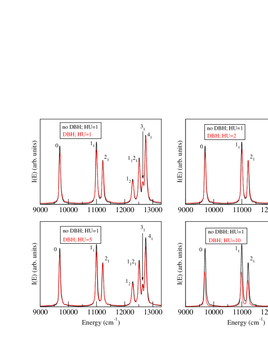
Figure 2: Comparison between the power spectrum obtained for CH₄ calculating all Hessians (no DBH; HU=1, black line) and those employing the DBH technique (top left panel, red line) and DBH in connection with Hessian Update schemes with different periodicities (other panels, red lines).

An examination of the frequencies of vibration reported in Table 5 leads to the observation that results obtained by means of the database technique are in good agreement with the standard approach in which all Hessians are calculated. The accuracy starts to diminish, especially regarding the ZPE value, for the DBH; HU=10 case. This was already clear from the bottom right panel of Figure 2, in which a loss in signal intensity is detected, an aspect related to the high percentage of rejected trajectories. The full widths at half maximum (FWHM) of the peaks are reported to provide a rough estimate of data uncertainty, and frequency estimates are generally well within the tolerance interval.

Table 5: Vibrational frequencies and ZPE for CH₄ in cm^-1. FWHM values (cm^-1) are given in parentheses. Column 1 indicates the vibrational transition (0 represents the ground state). Column 2 is reserved to the quantum mechanical (QM) benchmark values from Ref.84. Column 3 reports the outcomes of the all-Hessian simulation. The last four columns contain the results of DBH simulations. In the last row the mean absolute error (MAE) in cm^-1 with respect to QM results is given. FWHM values are not available for the 0$\rightarrow$ 3₁ transition.

Transition	QM	no DBH; HU=1	DBH; HU=1	DBH; HU=2	DBH; HU=5	DBH; HU=10
0$\rightarrow$ 11	1313	1302 (68)	1301 (72)	1301 (73)	1303 (69)	1304 (71)
0$\rightarrow$ 21	1535	1529 (69)	1528 (77)	1528 (75)	1529 (71)	1529 (80)
0$\rightarrow$ 12	2624	2592 (87)	2590 (95)	2591 (92)	2592 (92)	2599 (91)
0$\rightarrow$ 1121	2836	2820 (78)	2818 (83)	2818 (80)	2819 (78)	2820 (85)
0$\rightarrow$ 31	2949	2948	2945	2943	2942	2938
0$\rightarrow$ 41	3053	3053 (76)	3051 (79)	3050 (80)	3050 (81)	3050 (93)
ZPE	9707	9694 (65)	9699 (71)	9699 (69)	9690 (65)	9677 (68)
MAE	-	11.3	12.1	12.4	13.1	14.3

Glycine

Moving to “on-the-fly” applications, we employed the database approach to study the vibrational frequencies of glycine in full dimensionality (24 degrees of freedom). Calculations were based on a single, 2500-step long trajectory with a time step of 10 a.u. Ab initio molecular dynamics was performed at harmonic ZPE at DFT-B3LYP level of theory with aVDZ basis set, in agreement with a previous semiclassical study of glycine.(Gabas, Conte, and Ceotto, 2017) For the test of the determinant of the monodromy matrix we used a threshold equal to 10^-2. Furthermore, a well-established regularization technique for the monodromy matrix(Di Liberto and Ceotto, 2016) was adopted to avoid discard of the trajectory before its scheduled end. As anticipated in Section II, when performing SC spectroscopy “on-the-fly”, Hessian matrices are calculated once the entire trajectory has already been determined. This allows one to exploit DBH to reduce the number of Hessian calculations similarly to HU schemes but in a more flexible way.

Table 6: ZPE energies and frequencies of fundamental transitions of glycine (cm^-1). MAE values (cm^-1) are determined with respect to the SC simulation with all Hessians calculated ab initio (all Hess). Columns 3-5 report the outcomes of DBH calculations based on several sets of ab initio Hessians. The last three columns provide estimates obtained with the HU scheme. Numbers in parentheses are the FWHM (cm^-1) of the associate Fourier transform signal and their average is reported in the last row.

Mode	All Hess	DBH = 3.89	DBH = 7.62	DBH = 12.69	HU = 4	HU = 8	HU=13
24	3639 (55)	3639 (56)	3639 (60)	3639 (59)	3639 (55)	3636 (60)	3637 (73)
23	3372 (59)	3372 (83)	3369 (60)	3369 (48)	3372 (60)	3363 (70)	3370 (88)
22	3375 (58)	3378 (59)	3375 (61)	3378 (67)	3375 (59)	3372 (64)	3370 (82)
21	2904 (59)	2904 (59)	2904 (61)	2904 (62)	2901 (59)	2898 (61)	2895 (72)
20	2904 (53)	2907 (53)	2901 (55)	2904 (57)	2904 (54)	2901 (57)	2902 (78)
19	1779 (54)	1779 (53)	1782 (61)	1779 (58)	1779 (54)	1779 (60)	1777 (60)
18	1662 (52)	1662 (52)	1662 (46)	1668 (47)	1662 (50)	1656 (51)	1645 (60)
17	1404 (52)	1404 (53)	1404 (66)	1401 (57)	1404 (54)	1401 (63)	1405 (61)
16	1380 (66)	1383 (69)	1386 (68)	1383 (78)	1380 (67)	1383 (66)	1378 (62)
15	1344 (55)	1347 (56)	1350 (59)	1347 (60)	1344 (56)	1347 (56)	1342 (57)
14	1287 (85)	1287 (95)	1281 (68)	1287 (100)	1284 (86)	1275 (75)	1258 (78)
13	1158 (56)	1161 (57)	1164 (67)	1158 (64)	1158 (57)	1161 (60)	1159 (60)
12	1122 (53)	1125 (53)	1131 (57)	1134 (43)	1122 (53)	1125 (53)	1120 (51)
11	1098 (59)	1101 (60)	1101 (62)	1098 (68)	1098 (59)	1098 (63)	1096 (71)
10	900 (55)	900 (55)	903 (63)	900 (61)	900 (55)	900 (60)	899 (60)
9	879 (54)	879 (53)	882 (70)	876 (64)	879 (51)	882 (62)	880 (62)
8	798 (53)	798 (54)	801 (61)	798 (59)	798 (53)	798 (58)	796 (59)
7	654 (53)	654 (57)	663 (57)	657 (64)	654 (54)	657 (53)	652 (50)
6	621 (53)	621 (52)	621 (59)	621 (57)	621 (52)	621 (57)	619 (58)
5	489 (56)	492 (56)	492 (65)	498 (63)	489 (57)	489 (59)	491 (65)
4	456 (59)	456 (59)	456 (67)	456 (68)	456 (60)	453 (65)	454 (72)
3	252 (50)	252 (49)	252 (56)	252 (53)	252 (50)	249 (56)	254 (62)
2	201 (75)	201 (83)	204 (68)	204 (105)	201 (76)	198 (75)	193 (87)
1	78 (54)	78 (54)	81 (65)	78 (56)	78 (55)	81 (59)	79 (53)
ZPE	17164 (46)	17188 (55)	17185 (62)	17230 (57)	17161 (55)	17146 (58)	17046 (63)
MAE	-	2.1	3.8	4.7	0.4	3.8	8.8
MFWHM	57	59	62	63	58	61	66

All the results presented in Table 6 have excellent accuracy with respect to the benchmark semiclassical calculation based on 2500 ab initio Hessians. FWHM data further demonstrate the reliability of the various approximations. Due to the length of the dynamics ($\approx$ 0.6 ps), the lower bound to the FWHM values of the Fourier transform signal is about 30 cm^-1. Results show that most of them are actually in the 50-60 cm^-1 range and occasionally larger. The main reasons for such an enlargement, which apply also to the case of methane, lie in nearby states contributing to the power spectrum and to spurious rotations due to the adoption for SC calculations of a normal mode reference frame based on the equilibrium geometry. Both the database approach and the HU Bofill scheme are accurate, but DBH appears more stable and deteriorates in accuracy more slowly as fewer Hessian calculations are performed ab initio. To better appreciate this point and the comparison among the two approaches, the ratio (R) between the maximum of 2500 Hessians and the number of those actually calculated ab initio is indicated in the header of DBH columns (DBH=R). More specifically, data in column 3 of Table 6 are based on 643 ab initio Hessians, the ones in column 4 on 328 Hessians, and those in column 5 on 197 Hessians. The corresponding saving with respect to the total simulation time (including generation of the dynamics) of the all-Hessian simulations is equal to about 70%, 82%, and 88% respectively.

N-Acetyl-L-Phenylalaninyl-L-Methionine Amide

Our final spectroscopic study was dedicated to the challenging 46-atom N-acetyl-L-phenylalaninyl-L-methionine amide. The L-phenylalaninyl-L-methionine dipeptide (Phe-Met) is a prototypical system of proteins in which several hydrogen bonds govern the secondary and tertiary structures. In particular, there are three different H-bonds which are crucial in the stabilization of the folded structure: Two of them, an NH—$\pi$ in the phenylalaninyl and an NH—S in the methionine, are confined within the lateral chain of the aminoacids, while the third one is established between the NH₂ and C=O of the terminal groups. Biswal et al. have studied recently the conformation and the vibrational spectrum of the amide of this dipeptide capped with acetyl (Ac-Phe-Met-NH₂). They presented quantum DFT-D calculations together with gas-phase experiments, showing that the hydrogen bond involving the sulfur atom has a strength similar to that of the intrabackbone NH—O=C hydrogen bond.(Biswal et al., 2012)
Based on the satisfactory results obtained for the previous systems, we decided to employ the DBH approach. In fact, such a big and complex molecule could not be investigated with reasonable computational effort by means of the standard, all-Hessian SC procedure. DBH made the computational overhead affordable, and we were able to undertake a study based on ab initio “on-the-fly” semiclassical dynamics at DFT-B3LYP-D level of theory and 6-31G* basis set of the high energy quantum fundamentals of vibration. These include the 2 stretches involving the NH₂ group (sNH₂ and aNH₂) plus the two NH stretches, labeled NH(I) and NH(II). We identified the conformation illustrated in Fig. 3 as the most stable one, and normal modes were determined for this geometry.

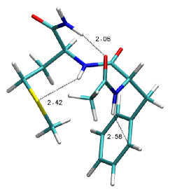
Figure 3: Global minimum of N-acetyl-L-phenylalaninyl-L-methionine amide at DFT-B3LYP-D level of theory with 6-31G* basis set. Hydrogen bonds are indicated by dashed lines.

As in the case of glycine, we performed ab initio calculations by means of the NWChem suite of codes,(Valiev et al., 2010) but this time the MC-DC-SCIVR approach was employed. Following the standard MC-DC-SCIVR recipe, we ran four simulations tailored on the four normal modes of interest. The starting conditions were chosen to be the equilibrium geometry for positions, while initial momenta were assigned according to the harmonic ZPE with an additional quantum of harmonic excitation for the mode under investigation. The reference states were chosen as described in Eq. (6) to enhance the signal corresponding to the target mode. All the trajectories were evolved for a total of about 0.6 ps. The subspace partition was obtained in agreement with the Hessian criterion(Di Liberto, Conte, and Ceotto, 2018b) and monodimensional subspaces were determined for all four modes. DBH was employed with $\rho=0.15$, which led to the construction of databases of less than 300 Hessians.

The molecule is made of 132 vibrational degrees of freedom with nine of them characterized by harmonic frequencies below 100 cm^–1, 16 in the 1500-1800 cm^-1 range, and 19 between 3000 and 3215 cm^-1. It is then clear that the density of vibrational states is very high and diffuse in the 3300-3600 cm^-1 interval investigated in this work, which includes (in addition to the four high frequency fundamentals) a large number of overtones and combination bands. Consequently some bands, due to resonances and dependent on the SC propagator (i.e. the trajectory) and the reference state, rather than well isolated peaks are expected in the power spectra. Furthermore, we found that for mode NH(I) the spectrum was very noisy due to the many couplings to other modes, and a reliable frequency estimate was not achievable. For this mode we ran a trajectory with tailored reference state at the lower harmonic ZPE to help weaken the couplings. It is known that such a simulation yields generally less accurate (even if still acceptable) frequencies, but the outcome was in this case proved to be satisfactory. Power spectra obtained from the several simulations previously described are reported in Fig. 4, where labels indicating the vibrational modes are written next to the relevant spectral signal.

Figure 4: MC-DC-SCIVR power spectra for the 4 highest frequency fundamentals of Ac-Phe-Met-NH₂. Vertical bars indicate experimental values.

The corresponding semiclassical frequencies are reported in Tab. 7 together with experimental results and harmonic estimates. FWHM values are given in parentheses. While harmonic values are substantially off the mark, the discrepancy between semiclassical values and the experiment is generally about 30 cm^-1. The distance is bigger for the NH(II) mode, which features a double peak. The lower frequency signal has been assigned to NH(II), while the other peak has been assigned to the signal of the coupled sNH₂ mode estimated in an approximate way using the SC propagator tailored for the NH(II) mode.

Table 7: Experimental, MC-DC-SCIVR, and harmonic frequencies of Ace-Phe-Met-NH₂. FWHM data are reported in parenthesis. All values are in cm^-1.

mode	Exp.(Biswal et al., 2012)	MC-DC SCIVR	Harm
aNH2	3520	3490 (47)	3682
NH(I)	3452	3480 (70)	3607
NH(II)	3363	3300 (45)	3568
sNH2	3388	3360 (45)	3535
MAE	-	37	167

IV Summary and Conclusions

We have introduced an innovative strategy to ease the calculation of Hessian matrices required by semiclassical spectroscopy. It is based on the idea that similar Hessians are likely to be derived from similar geometries, and it consists in the dynamical construction of a database of Hessian matrices and associated geometries. The other Hessians needed are approximated by database records according to a given threshold parameter accounting for the similarity of the instantaneous geometry to those in the database. This novel approach is midway between the single-Hessian approximation recently introduced in thawed Gaussian semiclassical vibronic spectroscopy, which is generally not sufficiently accurate for vibrational spectroscopy, and the basic full-Hessian SC calculation, which is too computationally expensive for applications to medium-large systems.

For the same purpose some Hessian extrapolation schemes based on finite differences have been developed. They have been shown to work efficiently and satisfactorily for small molecules, but they depend on a linear (monodimensional) approximation and their accuracy may deteriorate in high dimensional applications. Furthermore, these Hessian update schemes require new Hessian calculations rigorously at a constant pace along the trajectory lacking the flexibility of the database approach.

We applied the DBH technique to methane, interfacing the method with the Hessian Update Bofill scheme. This has permitted us to keep excellent accuracy while calculating only about 6% of the Hessians needed by a regular simulation. However, the small dimensionality of the molecule did not lead to a substantial speed up since the time needed by the search algorithm offsets the time saved by the reduced number of Hessian calculations. In this regard, the database approach has demonstrated its power in applications to bigger molecules for which, in absence of a precise analytical PES, ab initio “on-the-fly” dynamics is necessary. A first investigation of this kind involved glycine and showed that DBH permits the preservation of very good accuracy, reducing the number of Hessian matrices by a factor of about 13 and total computational times by about 88%. Hessian update schemes provided good results too, but their accuracy deteriorated faster. The ultimate demonstration of the upgrade provided by DBH is represented by the final study of the high frequency power spectrum for Ac-Phe-Met-NH₂. DBH has permitted the semiclassical analysis of this 46-atom system, which otherwise would have not been attainable.

Upon analysis of the results, we notice that the eigenvalues estimated by DBH are losing accuracy much faster than frequencies which are obtained as a difference between eigenvalues. This aspect does not constitute a severe drawback when moving to high dimensional systems for which the DC-SCIVR technique must be employed. In fact, “divide and conquer” SCIVR approaches are themselves less accurate in estimating ZPE energies compared to frequencies of vibration, which are the actual target of investigation.

In perspective DBH will permit semiclassical studies of complex molecular and supramolecular systems. In particular, the increased size of calculable systems will enable the investigation of molecular solvation and molecular adsorption on surfaces.