Lepton flavour universality in charged-current $B$ decays

Abstract

Tests of lepton flavour universality in charged-current $B$ decays offer an excellent opportunity to test the Standard Model, and show hints of new physics in analyses performed by the LHCb, Belle and BaBar experiments. These proceedings present the results from the LHCb collaboration on measurements of $\mathcal{R}({{D}^{*}})$ and $\mathcal{R}({{J\mskip-3.0mu/\mskip-2.0mu\psi\mskip 2.0mu}})$. It also presents the latest semileptonic tag measurement of $\mathcal{R}({D})$ and $\mathcal{R}({{D}^{*}})$ by the Belle collaboration. The latest HFLAV average shows a discrepancy of 3.1$\sigma$ between the Standard Model predictions and combined measurements of $\mathcal{R}({D})$ and $\mathcal{R}({{D}^{*}})$.

I Introduction

In the Standard Model of particle physics (SM) it is assumed that there are three generations of fermions which are nearly identical copies of one another with the same gauge charge assignments, but different masses. This implies that all leptons couple universally to the gauge bosons, and that the only difference in their interactions is caused by the difference in mass. This is called lepton flavour universality (LFU) and can be tested by measuring ratios of decays, such that the Cabibbo-Kobayashi-Maskawa matrix elements, and the majority of the form factors, cancel in the ratio.

These proceedings focus on the measurements of LFU in charged-current $B$ decays, which are of the form ${b}\rightarrow{c}{\ell^{-}}{{\overline{\nu}}_{\ell}}$, commonly known as measurements of $\mathcal{R}({H_{c}})$. The ratio $\mathcal{R}({H_{c}})$ is defined as

$${\mathcal{R}({H_{c}})}=\frac{{\mathcal{B}}({H_{b}}\rightarrow{H_{c}}{\tau^{-}}{{\overline{\nu}}_{\tau}})}{{\mathcal{B}}({H_{b}}\rightarrow{H_{c}}\ell^{-}{{\overline{\nu}}_{\ell}})}\,,$$ (1)

where $H_{b}$ and $H_{c}$ are a $b$ and $c$ hadron, respectively, and $\ell$ is either an electron or muon. The semitauonic decay is called the signal channel, and the other decay is the normalisation channel. These tree-level processes are theoretically clean and are sensitive to new physics, such as charged Higgs bosons or leptoquarks Buttazzo et al. (2017). Up until the start of 2019, there was a discrepancy of 4$\sigma$ between the SM predictions and the combined measurements of $\mathcal{R}({D})$ and $\mathcal{R}({{D}^{*}})$.

There are two types of experiments that have measured the ratios $\mathcal{R}({H_{c}})$. The first are the $B$ factories BaBar and Belle, which were both located at $e^{+}e^{-}$ colliders running at the $\mathchar 28935\relax{(4S)}$ resonance to produce ${{B}^{+}}$ ${{B}^{-}}$ or ${B}^{0}$ ${\kern 1.79993pt\overline{\kern-1.79993ptB}{}}{}^{0}$ pairs. They have the advantage that $B$ mesons are produced in a clean environment with little background and that the well-constrained kinematics are very beneficial for reconstructing final states with neutrinos. The BaBar and Belle experiments finished data taking in 2008 and 2010 and collected 433$\mbox{\,fb}^{-1}$ and 711$\mbox{\,fb}^{-1}$ of data, respectively.

LFU in charged-current $B$ decays can also be measured at the LHCb experiment, which records data from $pp$ collisions at the LHC. The $b$ quarks are produced through gluon fusion and thus all $b$-hadron species are created: ${{B}^{+}}$, ${B}^{0}$, ${B}^{0}_{s}$, ${B}_{c}^{+}$ and ${\mathchar 28931\relax}^{0}_{b}$. The $b$ hadrons are strongly boosted, providing an excellent separation between production and decay vertices. However, the large amount of $b$ quarks created comes at the cost of large amounts of background. The LHCb experiment recorded 3$\mbox{\,fb}^{-1}$ of data in 2011–2012 at $\sqrt{s}$ =7–8 TeV (Run 1), and 6$\mbox{\,fb}^{-1}$ from 2015–2018 at $\sqrt{s}$ =13 TeV (Run 2).

II Measurements from LHCb

This section presents LHCb’s three measurements of LFU in charged-current $B$ decays.

II.1 Muonic $\mathcal{R}({{D}^{*}})$

Figure 1: Distributions of $\rm{m}_{\rm{miss}}^{2}$ (left) and $E_{\mu}^{*}$ (right) in the highest $q^{2}$ bin of the signal data, overlaid with the projections of the fit model from LHCb’s muonic $\mathcal{R}({{D}^{*}})$ measurement Aaij et al. (2015). The signal distributions are red, and the normalisation channel is blue.

The $\mathcal{R}({{D}^{*}})$ analysis Aaij et al. (2015) measure the ratio

$${\mathcal{R}({{D}^{*}})}=\frac{{\mathcal{B}}({{\kern 1.79993pt\overline{\kern-1.79993ptB}{}}{}^{0}}\rightarrow{{D}^{*+}}{\tau^{-}}{{\overline{\nu}}_{\tau}})}{\mathcal{B}({{\kern 1.79993pt\overline{\kern-1.79993ptB}{}}{}^{0}}\rightarrow{{D}^{*+}}{\mu^{-}}{{\overline{\nu}}_{\mu}})}\,.$$ (2)

In this analysis, the $\tau^{-}$ decay is reconstructed as $\tau^{-}$ $\rightarrow$ $\mu^{-}$ ${\overline{\nu}}_{\mu}$ ${\nu}_{\tau}$, which means that the signal and normalisation channel both have the same visible final state. This ensures the cancellation of many systematic uncertainties in the ratio, but also makes it hard to distinguish between the two channels. The decay modes are measured using a multidimensional template fit based on the three kinematic variables that discriminate most between signal and normalisation channels. These are the missing mass squared ($m_{\rm miss}^{2}$), the muon energy ($E_{\mu}^{*}$) and the squared four-momentum of the lepton pair ($q^{2}$), all computed in the $B$-meson rest frame. An approximation of the boost of the $B$ meson is made by assuming that the boost of the visible decay products along the $z$-axis is equal to that of the $B$ meson: $(\gamma\beta_{z})_{{B}}\approx(\gamma\beta_{z})_{{{D}^{*}}\mu}$

The analysis is performed using the Run 1 data set of LHCb. The results of the fit, in the highest $q^{2}$ bin, are shown in Fig 1. After correcting for the efficiencies of reconstructing the signal and normalisation mode, they yield a value of

$${\mathcal{R}({{D}^{*}})}=0.336\pm 0.027\mathrm{\,(stat)}\pm 0.030\mathrm{\,(syst)}\,.$$

The largest contribution to the systematic uncertainty is due to the limited size of the simulation samples used to create the template shapes. The obtained value of $\mathcal{R}({{D}^{*}})$ is compatible with the SM within 2.1$\sigma$.

II.2 Hadronic $\mathcal{R}({{D}^{*}})$

Figure 2: Fit projections of the three-dimensional fit of the 3$\pi$ decay time, $q^{2}$, and BDT output distributions from LHCb’s hadronic $\mathcal{R}({{D}^{*}})$ measurement Aaij et al. (2018a).

In the hadronic measurement of $\mathcal{R}({{D}^{*}})$ Aaij et al. (2018b, a) the $\tau^{-}$ lepton is reconstructed with three charged pions in the final state. Instead of the ${{\kern 1.79993pt\overline{\kern-1.79993ptB}{}}{}^{0}}\rightarrow{{D}^{*+}}{\mu^{-}}{{\overline{\nu}}_{\mu}}$ decay mode, this analysis uses the decay ${{\kern 1.79993pt\overline{\kern-1.79993ptB}{}}{}^{0}}\rightarrow{{D}^{*+}}{{\pi}^{-}}{{\pi}^{+}}{{\pi}^{-}}$ as a normalisation channel. It then measures the ratio $\mathcal{K}({{D}^{*}})$, which is defined as:

$$\mathcal{K}({{D}^{*}})=\frac{{\mathcal{B}}({{\kern 1.79993pt\overline{\kern-1.79993ptB}{}}{}^{0}}\rightarrow{{D}^{*+}}{\tau^{-}}{{\overline{\nu}}_{\tau}})}{{\mathcal{B}}({{\kern 1.79993pt\overline{\kern-1.79993ptB}{}}{}^{0}}\rightarrow{{D}^{*+}}{{\pi}^{-}}{{\pi}^{+}}{{\pi}^{-}})}\,.$$ (3)

To convert this value to $\mathcal{R}({{D}^{*}})$, $\mathcal{K}({{D}^{*}})$ is multiplied by the ratio of the branching ratios of the ${{\kern 1.79993pt\overline{\kern-1.79993ptB}{}}{}^{0}}\rightarrow{{D}^{*+}}{{\pi}^{-}}{{\pi}^{+}}{{\pi}^{-}}$ and ${{\kern 1.79993pt\overline{\kern-1.79993ptB}{}}{}^{0}}\rightarrow{{D}^{*+}}{\mu^{-}}{{\overline{\nu}}_{\mu}}$ decays, which are taken as external inputs from HFLAV average:

$${\mathcal{R}({{D}^{*}})}=\mathcal{K}({{D}^{*}})\times\left(\frac{{\mathcal{B}}({{\kern 1.79993pt\overline{\kern-1.79993ptB}{}}{}^{0}}\rightarrow{{D}^{*+}}{{\pi}^{-}}{{\pi}^{+}}{{\pi}^{-}})}{{\mathcal{B}}({{\kern 1.79993pt\overline{\kern-1.79993ptB}{}}{}^{0}}\rightarrow{{D}^{*+}}{\mu^{-}}{{\overline{\nu}}_{\mu}})}\right)\,.$$ (4)

This analysis benefits from the well-defined $\tau^{-}$ decay vertex which is downstream from the $B$ decay vertex, and suppresses backgrounds by exploiting this topology. For the signal channel a template fit is performed in three variable: the decay time of the three pions ($t_{\tau}$), $q^{2}$, and the output of a boosted decision tree (BDT). This BDT is used to suppress backgrounds coming from doubly-charmed ${{B}^{0}}\rightarrow{{D}^{*-}}{{D}^{+}_{s}}X$ decays, where $X={{{B}^{+}}},{{B}^{0}},{{B}^{0}_{s}}$. Projections of the fits for each of these variables are shown in Fig. 2. The analysis yields a value of

$$\mathcal{K}({{D}^{*}})=1.93\pm 0.12\mathrm{\,(stat)}\pm 0.17\mathrm{\,(syst)}\,.$$

Recently HFLAV updated the external input of the average of the measurements of ${\mathcal{B}}({{B}^{0}}\rightarrow{{D}^{*-}}{\ell^{+}}{{\nu}_{\ell}})$, which changed from $(4.88\pm 0.01\mathrm{\,(stat)}\pm 0.10\mathrm{\,(syst)})\%$ to $(5.08\pm 0.02\mathrm{\,(stat)}\pm 0.12\mathrm{\,(syst)})\%$. The change is largely due to the decision to no longer average over the ${D}^{*+}$ and ${D}^{*0}$ decays, resulting in the exclusion of measurements combining these states. Moreover, the new average includes the latest Belle measurement Abdesselam et al. (2018).

Using the updated HFLAV average, LHCb’s measurement of $\mathcal{R}({{D}^{*}})$ using the hadronic $\tau^{-}$ decay yields a value of:

$${\mathcal{R}({{D}^{*}})}=0.280\pm 0.018\mathrm{\,(stat)}\pm 0.029\mathrm{\,(syst)}\,.$$

This is in agreement with the SM within $1\sigma$.

II.3 Muonic $\mathcal{R}({{J\mskip-3.0mu/\mskip-2.0mu\psi\mskip 2.0mu}})$

The latest measurement from LHCb presented here Aaij et al. (2018c) studies the ratio in a different decay mode, namely

$${\mathcal{R}({{J\mskip-3.0mu/\mskip-2.0mu\psi\mskip 2.0mu}})}=\frac{{{B}_{c}^{+}}\rightarrow{{J\mskip-3.0mu/\mskip-2.0mu\psi\mskip 2.0mu}}{\tau^{+}}{{\nu}_{\tau}}}{{{B}_{c}^{+}}\rightarrow{{J\mskip-3.0mu/\mskip-2.0mu\psi\mskip 2.0mu}}{\mu^{+}}{{\nu}_{\mu}}}\,.$$ (5)

The $\tau^{-}$ lepton is reconstructed in the muonic decay mode and also in this analysis the signal and normalisation channel are distinguished in a three-dimensional templated fit based on the $\tau^{-}$ decay time, $m_{\rm miss}^{2}$, and the variable $Z({q^{2}},E_{\mu}^{*})$, which is a combination of the $q^{2}$ and $E_{\mu}^{*}$ variables. The same boost approximation is used as in the muonic $\mathcal{R}({{D}^{*}})$ analysis. Projections of the fit output are shown in Fig. 3.

The analysis yields a value of

$${\mathcal{R}({{J\mskip-3.0mu/\mskip-2.0mu\psi\mskip 2.0mu}})}=0.71\pm 0.17\mathrm{\,(stat)}\pm 0.18\mathrm{\,(syst)}\,,$$

where one of the largest systematic uncertainties comes from the limited knowledge on the form factors of the ${{B}_{c}^{+}}\rightarrow{{J\mskip-3.0mu/\mskip-2.0mu\psi\mskip 2.0mu}}{\ell^{+}}{{\nu}_{\ell}}$ decays. These are currently fit from data but can be significantly improved with new lattice calculations. $\mathcal{R}({{J\mskip-3.0mu/\mskip-2.0mu\psi\mskip 2.0mu}})$ is compatible with the SM within 2$\sigma$.

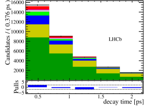
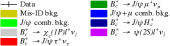
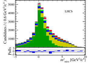
Figure 3: Fit projections of the $\tau$ decay time (left), $m_{\rm miss}^{2}$ (middle) and $Z({q^{2}},E_{\mu}^{*})$ variables in the measurement of $\mathcal{R}({{J\mskip-3.0mu/\mskip-2.0mu\psi\mskip 2.0mu}})$ from LHCb Aaij et al. (2018c).

III Latest measurement from Belle

The latest measurement of LFU in charged-current $B$ decays of the Belle collaboration Abdesselam et al. (2019) simultaneously measures $\mathcal{R}({D})$ and $\mathcal{R}({{D}^{*}})$. It analyses the full $\mathchar 28935\relax{(4S)}$ sample recorded by the Belle detector, consisting of $772\times 10^{6}$ $B$ ${\kern 1.79993pt\overline{\kern-1.79993ptB}{}}$ events. It uses a semileptonic tag, meaning that the other $B$ meson in the event is reconstructed in the semileptonic decay ${B}\rightarrow{D}^{(*)}\ell{{\nu}_{\ell}}$, where $\ell=e,\mu$. Since the previous $\mathcal{R}({{D}^{*}})$ analysis with a semileptonic tag Sato et al. (2016), the tagging algorithm has been extended with more reconstruction channels and now uses a BDT resulting in a sample with higher signal purity.

In order to make sure the tag $B$ meson does not decay with a $\tau^{-}$ lepton in the final state, a cut on the variable $\cos\theta_{{B},{D}^{(*)}\ell}$ is applied, where $\cos\theta_{{B},{D}^{(*)}\ell}$ is the cosine of the angle between the momentum of the $B$ meson and the ${D}^{(*)}\ell$ combination in the $\mathchar 28935\relax{(4S)}$ rest frame. This variable is reconstructed assuming that there is only one massless unreconstructed particle (neutrino) in the decay and it is defined as:

$$\cos\theta_{{B},{D}^{(*)}\ell}\equiv\frac{2E_{\rm beam}E_{{D}^{(*)}\ell}-m_{B}^{2}-m_{{D}^{(*)}\ell}^{2}}{2|p_{B}||p_{{D}^{(*)}\ell}|}\,,$$ (6)

where $E_{\rm beam}$ is the energy of the beam, and $E_{{D}^{(*)}\ell}$, $m_{{D}^{(*)}\ell}$, and $p_{{D}^{(*)}\ell}$ are the energy, mass and momentum of the ${D}^{(*)}\ell$ system, respectively. The variable $m_{B}$ is the nominal $B$ meson mass, and $p_{B}$ the $B$ meson momentum.

The $B$ mesons are reconstructed in the ${{D}^{+}}{\ell^{-}}$, ${{D}^{0}}{\ell^{-}}$, ${{D}^{*+}}{\ell^{-}}$ and ${{D}^{*0}}{\ell^{-}}$ decays, which increases the signal yields compared to the previous semileptoni-tag analysis by Belle Sato et al. (2016) because now both ${{B}^{+}}$ and ${B}^{0}$ decays are studied, rather than only ${B}^{0}$ decays. The ${D}^{*}$ mesons are reconstructed as ${{D}^{*+}}\rightarrow{{D}^{0}}{{\pi}^{+}}$, ${{D}^{*+}}\rightarrow{{D}^{+}}{{\pi}^{0}}$, and ${{D}^{*0}}\rightarrow{{D}^{0}}{{\pi}^{0}}$. The ${D}^{0}$ and ${D}^{+}$ mesons are reconstructed in various final states with kaons and pions, adding up 30% and 22% of the total ${D}^{0}$ and ${D}^{+}$ branching fractions, respectively. To reduce backgrounds, the $D$ candidates are required to be in a mass window within 15${\mathrm{\,Me\kern-1.00006ptV\!/}c^{2}}$ of their nominal mass, although this mass window is extended for $D$ mesons with a ${\pi}^{0}$ in the final state due to the worse resolution for these events. In every event, the two $B$ mesons are required to have opposite flavour to reduce combinatorial backgrounds.

For each of the four samples, a two-dimensional template fit is performed to distinguish signal, normalisation and background yields. The two parameters used to fit in are $E_{\rm ECL}$ and class. The former is the energy deposited in the calorimeter which is not associated with reconstructed particles. This energy, which is restricted to be less than 1.2$\mathrm{\,Ge\kern-1.00006ptV}$, peaks at zero for the signal and normalisation channels, while it has a reasonably flat distribution for the background components, as illustrated in Fig. 4. The class variable is the output of a BDT based on the visible energy $E_{\rm vis}$, $m_{\rm miss}^{2}$, and $\cos\theta_{{B},{D}^{(*)}\ell}$. No further selection is applied to this variable.

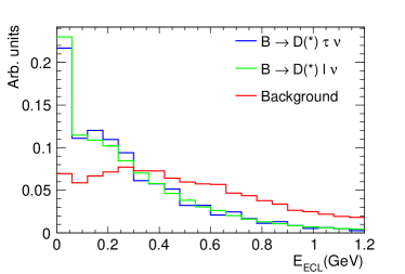
Figure 4: Distributions of the $E_{\rm ECL}$ variable used in Belle’s semileptonic tag measurement Abdesselam et al. (2019). The distributions of the signal, normalisation and background samples are taken from simulation and normalised to unity.

The fits are performed simultaneously on the four samples and consists of templates for the following components:

• ${D}^{(*)}\tau{{\nu}_{\tau}}$ ,

• ${D}^{(*)}\ell{{\nu}_{\ell}}$ ,

• ${D}^{**}\ell{{\nu}_{\ell}}$, where $D^{**}={D}_{1},{D}_{2}^{*},{D}_{1}^{{}^{\prime}},{D}_{0}^{*}$ ,

• feeddown from ${D}^{*}\ell{{\nu}_{\ell}}$ to ${D}\ell{{\nu}_{\ell}}$ decays ,

• fake ${D}^{(*)}$, fixed in the fit

• other backgrounds, fixed in fit

The fit PDFs are based on simulation samples which have a luminosity of ten times the total collected $B$ ${\kern 1.79993pt\overline{\kern-1.79993ptB}{}}$ luminosity for the signal and normalisation channels, and five times for the ${D}^{**}$ states. To get an estimate of the feed down, the result of the ${{D}^{*}}\ell$ (${{D}^{*}}\tau$) fit is used to constrain this component in the ${D}\ell$ (${D}\tau$) fit. The number of fake ${D}^{(*)}$ decays is determined from the $\Delta m=m_{{{D}^{*}}}-m_{{D}}$ sidebands and the yields of the other backgrounds are fixed to their simulation expectation value.

Fit projections of the $D^{+}\ell^{-}$ and $D^{0}\ell^{-}$ samples are shown in Fig. 6. The blue signal samples are hardly visible in the plots on the left showing the full classifier region. To illustrate the region associated with signal, also the fit results for the region with class $>0.9$ are shown in Fig. 6 (right). Here, the signal is much more visible, and the contribution of the normalisation channel is reduced. Fig. 7 shows similar plots, but for the ${{D}^{*+}}{\ell^{-}}$ and ${{D}^{*0}}{\ell^{-}}$ samples.

Finally, $\mathcal{R}(D^{(*)})$ can be calculated using the following expression:

$$\mathcal{R}(D^{(*)})=\frac{1}{2\mathcal{B}({\tau^{-}}\rightarrow{\ell^{-}}{{\overline{\nu}}_{\ell}}{{\nu}_{\tau}})}\cdot\frac{\varepsilon_{\rm norm}}{\varepsilon_{\rm sig}}\cdot\frac{N_{\rm sig}}{N_{\rm norm}}\,,$$ (7)

where $\varepsilon_{\rm sig(norm)}$ and $N_{\rm sig(norm)}$ are the detection efficiency and fitted yields of the signal and normalisation modes, respectively. $\mathcal{B}({\tau^{-}}\rightarrow{\ell^{-}}{{\overline{\nu}}_{\ell}}{{\nu}_{\tau}})$ is the world average for $\ell=e,\mu$. The efficiencies are taken from simulation samples, which are corrected to resemble the data more closely by applying correction factors. One of the largest corrections is to the lepton identification efficiency, which is corrected separately for electrons and muons. The efficiencies are corrected based on their kinematical dependence using control samples of ${e^{+}e^{-}}\rightarrow{e^{+}e^{-}}\ell^{+}\ell^{-}$ and ${{J\mskip-3.0mu/\mskip-2.0mu\psi\mskip 2.0mu}}\rightarrow\ell^{+}\ell^{-}$ decays.

The analysis measures values of

$${\mathcal{R}({D})} =0.307\pm 0.037\mathrm{\,(stat)}\pm 0.016\mathrm{\,(syst)}\,,$$

$${\mathcal{R}({{D}^{*}})} =0.283\pm 0.018\mathrm{\,(stat)}\pm 0.014\mathrm{\,(syst)}\,,$$

where the correlation between the statistical uncertainties and between the systematic uncertainties is $-0.53$ and $-0.52$, respectively. These are the most precise measurements of $\mathcal{R}({D})$ and $\mathcal{R}({{D}^{*}})$ to date and they are in agreement with the SM within 0.2$\sigma$ and 1.1$\sigma$, respectively. The combined result agrees with the SM prediction within 1.2$\sigma$. The largest contributions to the systematic uncertainties come from the limited size of the simulation sample, and the knowledge on the reconstruction efficiency.

IV Conclusions

The HFLAV group produced new averages of all measurements of $\mathcal{R}({D})$ and $\mathcal{R}({{D}^{*}})$, including the latest result from Belle and the update of the external input for LHCb’s hadronic $\mathcal{R}({{D}^{*}})$ measurement. The current averages are:

$${\mathcal{R}({D})} =0.349\pm 0.027\mathrm{\,(stat)}\pm 0.015\mathrm{\,(syst)}\,,$$

$${\mathcal{R}({{D}^{*}})} =0.298\pm 0.011\mathrm{\,(stat)}\pm 0.007\mathrm{\,(syst)}\,.$$

The combination of all measurements of $\mathcal{R}({D})$ and $\mathcal{R}({{D}^{*}})$, which is shown in Fig. 5, yields a 3.1$\sigma$ discrepancy with the SM.

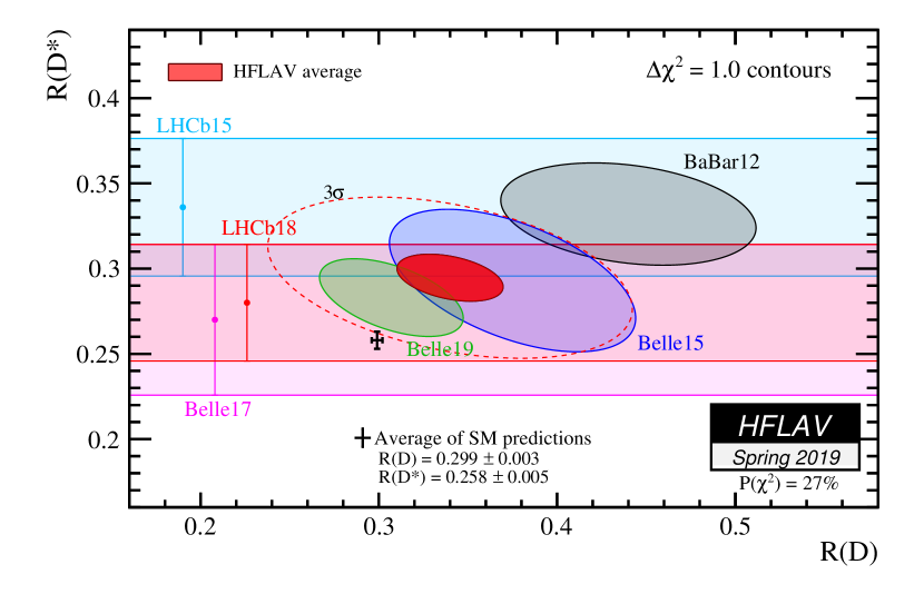
Figure 5: HFLAV average of all measurements of $\mathcal{R}({D})$ and $\mathcal{R}({{D}^{*}})$, updated with the results of the Belle collaboration presented in these proceedings. The red ellipse shows the combined average and the data point is the SM prediction, showing a discrepancy of 3.1$\sigma$. This plot is retrieved from the HFLAV website Amhis et al. (2017), using inputs from Lees et al. (2012, 2013); Huschle et al. (2015); Aaij et al. (2015); Hirose et al. (2017, 2018); Aaij et al. (2018b, a); Abdesselam et al. (2019).

Many new measurements of LFU in charged-current $B$ decays in LHCb are on their way. Work is ongoing on updates of the measurements presented in these proceedings, including the extension of the muonic $\mathcal{R}({{D}^{*}})$ measurement to the combination of $\mathcal{R}({D})$-$\mathcal{R}({{D}^{*}})$. Additionally, other decay channels are being studied, these measure the ratios $\mathcal{R}({{D}^{+}})$, $\mathcal{R}({{\mathchar 28931\relax}^{+}_{c}})$, $\mathcal{R}({{D}^{+}_{s}})$, $\mathcal{R}({p}{p})$. They are analysed both in muonic and hadronic decay mode of the $\tau^{-}$ lepton, and, depending on the measurement, use the Run 2 as well as the Run 1 dataset. These measurements will shed new light on the current discrepancy with the SM. Finally, the large datasets that will be collected by the LHCb upgrade Aaij et al. (2018d) and Belle II Altmannshofer et al. (2018) experiments will allow measurements of LFU in charged-current $B$ decays to be precise enough to confirm LFU breaking if the central values remain the same as the current best-fit values.

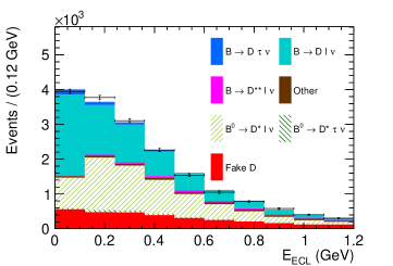
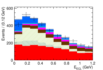
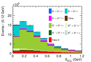
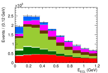
Figure 6: Fit projections of the $D^{+}\ell^{-}$ (top) and $D^{0}\ell^{-}$ (bottom) samples as a function of $E_{\rm ECL}$ Abdesselam et al. (2019). The plots on the left show the full classifier region, while the plots on the right are the signal region, defined by the selection class $>0.9$.

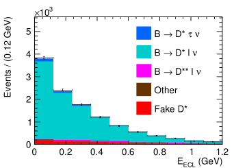
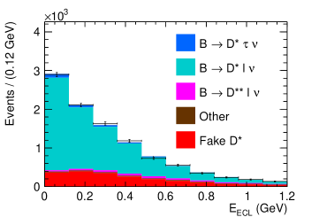
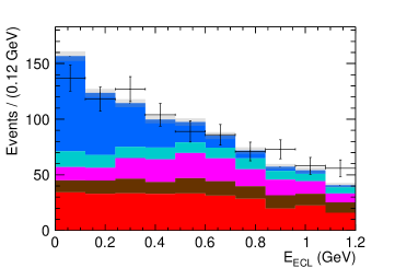
Figure 7: Fit projections of the $D^{\ast+}\ell^{-}$ (top) and $D^{\ast 0}\ell^{-}$ (bottom) samples as a function of $E_{\rm ECL}$ Abdesselam et al. (2019). The plots on the left show the full classifier region, while the plots on the right are the signal region, defined by the selection class $>0.9$.

References

- Buttazzo et al. (2017) D. Buttazzo, A. Greljo, G. Isidori, and D. Marzocca, JHEP 11, 044 (2017), eprint 1706.07808.
- Aaij et al. (2015) R. Aaij et al. (LHCb), Phys. Rev. Lett. 115, 111803 (2015), [Erratum: Phys. Rev. Lett.115,no.15,159901(2015)], eprint 1506.08614.
- Aaij et al. (2018a) R. Aaij et al. (LHCb), Phys. Rev. D97, 072013 (2018a), eprint 1711.02505.
- Aaij et al. (2018b) R. Aaij et al. (LHCb), Phys. Rev. Lett. 120, 171802 (2018b), eprint 1708.08856.
- Abdesselam et al. (2018) A. Abdesselam et al. (Belle) (2018), eprint 1809.03290.
- Aaij et al. (2018c) R. Aaij et al. (LHCb), Phys. Rev. Lett. 120, 121801 (2018c), eprint 1711.05623.
- Abdesselam et al. (2019) A. Abdesselam et al. (Belle) (2019), eprint 1904.08794.
- Sato et al. (2016) Y. Sato et al. (Belle), Phys. Rev. D94, 072007 (2016), eprint 1607.07923.
- Amhis et al. (2017) Y. Amhis et al. (Heavy Flavor Averaging Group), Eur. Phys. J. C77, 895 (2017), updated results and plots available at https://hflav.web.cern.ch, eprint 1612.07233.
- Lees et al. (2012) J. P. Lees et al. (BaBar), Phys. Rev. Lett. 109, 101802 (2012), eprint 1205.5442.
- Lees et al. (2013) J. P. Lees et al. (BaBar), Phys. Rev. D88, 072012 (2013), eprint 1303.0571.
- Huschle et al. (2015) M. Huschle et al. (Belle), Phys. Rev. D92, 072014 (2015), eprint 1507.03233.
- Hirose et al. (2017) S. Hirose et al. (Belle), Phys. Rev. Lett. 118, 211801 (2017), eprint 1612.00529.
- Hirose et al. (2018) S. Hirose et al. (Belle), Phys. Rev. D97, 012004 (2018), eprint 1709.00129.
- Aaij et al. (2018d) R. Aaij et al. (LHCb) (2018d), eprint 1808.08865.
- Altmannshofer et al. (2018) W. Altmannshofer et al. (Belle-II) (2018), eprint 1808.10567.