Themis: Fair and Efficient GPU Cluster Scheduling

Abstract: Modern distributed machine learning (ML) training workloads benefit significantly from leveraging GPUs. However, significant contention ensues when multiple such workloads are run atop a shared cluster of GPUs. A key question is how to fairly apportion GPUs across workloads. We find that established cluster scheduling disciplines are a poor fit because of ML workloads’ unique attributes: ML jobs have long-running tasks that need to be gang-scheduled, and their performance is sensitive to tasks’ relative placement.

We propose Themis, a new scheduling framework for ML training workloads. It’s GPU allocation policy enforces that ML workloads complete in a finish-time fair manner, a new notion we introduce. To capture placement sensitivity and ensure efficiency, Themis uses a two-level scheduling architecture where ML workloads bid on available resources that are offered in an auction run by a central arbiter. Our auction design allocates GPUs to winning bids by trading off efficiency for fairness in the short term, but ensuring finish-time fairness in the long term. Our evaluation on a production trace shows that Themis can improve fairness by more than $2.25X$ and is  $5\%$ to $250$% more cluster efficient in comparison to state-of-the-art schedulers.

1 Introduction

With the widespread success of machine learning (ML) for tasks such as object detection, speech recognition, and machine translation, a number of enterprises are now incorporating ML models into their products. Training individual ML models is time- and resource-intensive with each training job typically executing in parallel on a number of GPUs.

With different groups in the same organization training ML models, it is beneficial to consolidate GPU resources into a shared cluster. Similar to existing clusters used for large scale data analytics, shared GPU clusters for ML have a number of operational advantages, e.g., reduced development overheads, lower costs for maintaining GPUs, etc. However, today, there are no ML workload-specific mechanisms to share a GPU cluster in a fair manner.

Our conversations with cluster operators indicate that fairness is crucial; specifically, that sharing an ML cluster becomes attractive to users only if they have the appropriate sharing incentive. That is, if there are a total $N$ users sharing a cluster $C$, every user’s performance should be no worse than using a private cluster of size $\frac{C}{N}$. Absent such incentive, users are either forced to sacrifice performance and suffer long wait times for getting their ML jobs scheduled, or abandon shared clusters and deploy their own expensive hardware.

Providing sharing incentive through fair scheduling mechanisms has been widely studied in prior cluster scheduling frameworks, e.g., Quincy [18], DRF [8], and Carbyne [11]. However, these techniques were designed for big data workloads, and while they are used widely to manage GPU clusters today, they are far from effective.

The key reason is that ML workloads have unique characteristics that make existing “fair” allocation schemes actually unfair. First, unlike batch analytics workloads, ML jobs have long running tasks that need to be scheduled together, i.e., gang-scheduled. Second, each task in a job often runs for a number of iterations while synchronizing model updates at the end of each iteration. This frequent communication means that jobs are placement-sensitive, i.e., placing all the tasks for a job on the same machine or the same rack can lead to significant speedups. Equally importantly, as we show, ML jobs differ in their relative placement-sensitivity (Section 3.1.2).

In Section 3, we show that having long-running tasks means that established schemes such as DRF – which aims to equally allocate the GPUs released upon task completions – can arbitrarily violate sharing incentive. We show that even if GPU resources were released/reallocated on fine time-scales [13], placement sensitivity means that jobs with same aggregate resources could have widely different performance, violating sharing incentive. Finally, heterogeneity in placement sensitivity means that existing scheduling schemes also violate Pareto efficiency and envy-freedom, two other properties that are central to fairness [35].

Our scheduler, Themis, address these challenges, and supports sharing incentive, Pareto efficiency, and envy-freedom for ML workloads. It multiplexes a GPU cluster across ML applications (Section 2), or apps for short, where every app consists of one or more related ML jobs, each running with different hyper-parameters, to train an accurate model for a given task. To capture the effect of long running tasks and placement sensitivity, Themis uses a new long-term fairness metric, finish-time fairness, which is the ratio of the running time in a shared cluster with $N$ apps to running alone in a $\frac{1}{N}$ cluster. Themis’s goal is thus to minimize the maximum finish time fairness across all ML apps while efficiently utilizing cluster GPUs. We achieve this goal using two key ideas.

First, we propose to widen the API between ML apps and the scheduler to allow apps to specify placement preferences. We do this by introducing the notion of a round-by-round auction. Themis uses leases to account for long-running ML tasks, and auction rounds start when leases expire. At the start of a round, our scheduler requests apps for their finish-time fairness metrics, and makes all available GPUs visible to a fraction of apps that are currently farthest in terms of their fairness metric. Each such app has the opportunity to bid for subsets of these GPUs as a part of an auction; bid values reflect the app’s new (placement sensitive) finish time fairness metric from acquiring different GPU subsets. A central arbiter determines the global winning bids to maximize the aggregate improvement in the finish time fair metrics across all bidding apps. Using auctions means that we need to ensure that apps are truthful when they bid for GPUs. Thus we use a partial allocation auction that incentivizes truth telling, and ensures Pareto-efficiency and envy-freeness by design.

While a far-from-fair app may lose an auction round, perhaps because it placed less ideally than another app, its bid values for subsequent auctions naturally increase (because a losing app’s finish time fairness worsens), thereby improving the odds of it winning future rounds. Thus, our approach converges to fair allocations over the long term, while staying efficient and placement-sensitive in the short term.

Second, we present a two-level scheduling design that contains a centralized inter-app scheduler at the bottom level, and a narrow API to integrate with existing hyper-parameter tuning frameworks at the top level. A number of existing frameworks such as Hyperdrive [30] and HyperOpt [3] can intelligently apportion GPU resources between various jobs in a single app, and in some cases also terminate a job early if its progress is not promising. Our design allows apps to directly use such existing hyper parameter tuning frameworks. We describe how Themis accommodates various hyper-parameter tuning systems and how its API is exercised in extracting relevant inputs from apps when running auctions.

We implement Themis atop Apache YARN 3.2.0, and evaluate by replaying workloads from a large enterprise trace. Our results show that Themis is atleast $2.25X$ better than state-of-the-art schedulers while also improving cluster efficiency by  $5$% to $250$%. To further understand our scheduling decisions, we perform an event-driven simulation using the same trace, and our results show that Themis offers greater benefits when we increase the fraction of network intensive apps, and the cluster contention.

2 Motivation

We start by defining the terminology used in the rest of the paper. We then study the unique properties of ML workload traces from a ML training GPU cluster at a large software company. We end by stating our goals based on our trace analysis and conversations with the cluster operators.

2.1 Preliminaries

We define an ML app, or simply an “app”, as a collection of one or more ML model training jobs. Each app corresponds to a user training an ML model for a high-level goal, such as speech recognition or object detection. Users train these models knowing the appropriate hyper-parameters (in which case there is just a single job in the app), or they train a closely related set of models ($n$ jobs) that explore hyper-parameters such as learning rate, momentum etc. [30, 22] to identify and train the best target model for the activity at hand.

Each job’s constituent work is performed by a number of parallel tasks. At any given time, all of a job’s tasks collectively process a mini-batch of training data; we assume that the size of the batch is fixed for the duration of a job. Each task typically processes a subset of the batch, and, starting from an initial version of the model, executes multiple iterations of the underlying learning algorithm to improve the model. We assume all jobs use the popular synchronous SGD [4].

We consider the finish time of an app to be when the best model and relevant hyper-parameters have been identified. Along the course of identifying such a model, the app may decide to terminate some of its constituent jobs early [30, 3]; such jobs may be exploring hyper-parameters that are clearly sub-optimal (the jobs’ validation accuracy improvement over iterations is significantly worse than other jobs in the same app). For apps that contain a single job, finish time is the time taken to train this model to a target accuracy or maximum number of iterations.

2.2 Characterizing Production ML Apps

Figure 1: Aggregate GPU demand of ML apps over time

Figure 2: Job count distribution across different apps

Figure 3: ML app time ( = total GPU time across all jobs in app) distribution

Figure 4: Distribution of Task GPU times

We perform an analysis of the properties of GPU-based ML training workloads by analyzing workload traces obtained from a large internet company. The GPU cluster we study supports over 5000 unique users. We restrict our analysis to a subset of the trace that contains 85 ML training apps submitted using a hyper-parameter tuning framework.

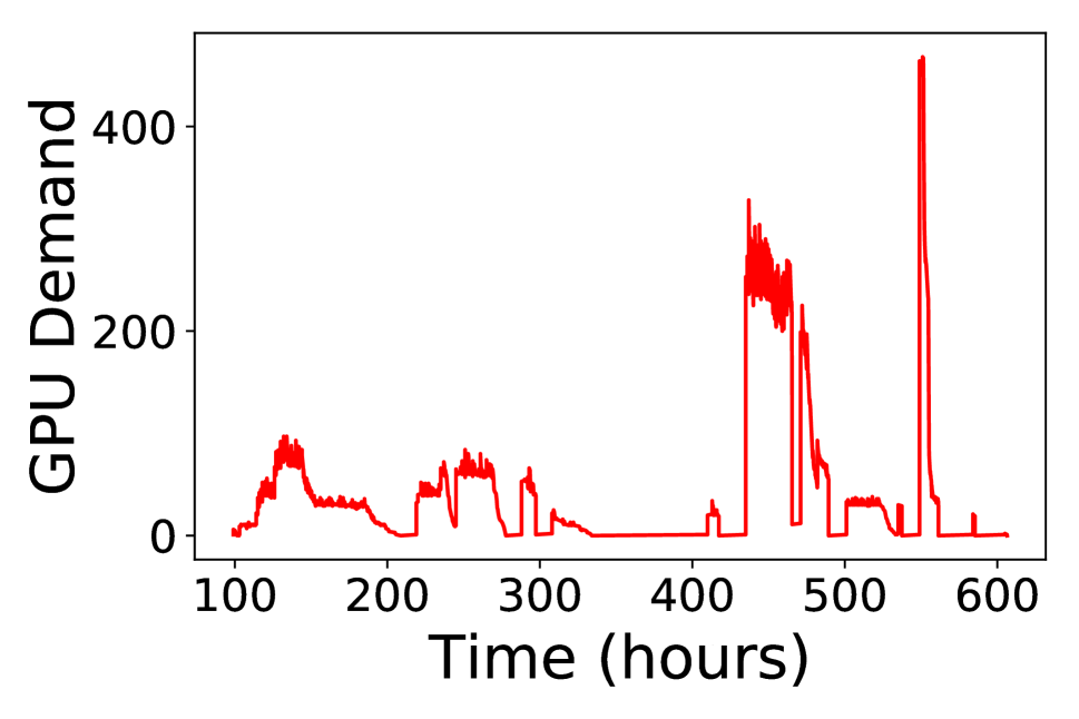
GPU clusters are known to be heavily contented [19], and we find this also holds true in the subset of the trace of ML apps we consider (Figure 4). For instance, we see that GPU demand is bursty and the average GPU demand is ~50 GPUs.

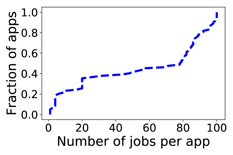
We also use the trace to provide a first-of-a-kind view into the characteristics of ML apps. As mentioned in Section 2.1, apps may either train a single model to reach a target accuracy (1 job) or may use the cluster to explore various hyper-parameters for a given model (n jobs). Figure 4 shows that ~10% of the apps have 1 job, and around ~90% of the apps perform hyper-parameter exploration with as many as 100 jobs (median of 75 jobs). Interestingly, there is also a significant variation in the number of hyper-parameters explored ranging from a few tens to about a hundred (not shown).

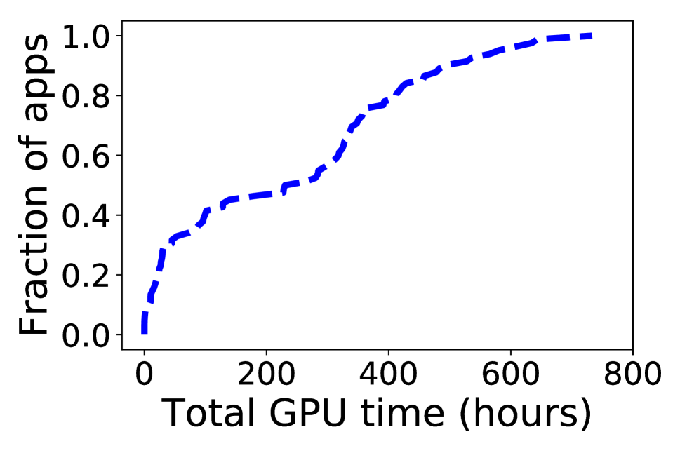
We also measure the GPU time of all ML apps in the trace. If an app uses 2 jobs with 2 GPUs each for a period of 10 minutes, then the task GPU times would be 10 minutes each, the job GPU times would be 20 minutes each, and the app GPU time would be 40 GPU minutes. Figure 4 and Figure 4 show the long running nature of ML apps: the median app takes 11.5 GPU days and the median task takes 3.75 GPU hours. There is a wide diversity with a significant fraction of jobs and apps that are more than 10X shorter and many that are more than 10X longer.

From our analysis we see that ML apps are heterogeneous in terms of resource usage, and number of jobs submitted. Running times are also heterogeneous, but at the same time much longer than, e.g., running times of big data analytics jobs (typical a few hours [12]). Handling such heterogeneity can be challenging for scheduling frameworks, and the long running nature may make controlling app performance particularly difficult in a shared setting with high contention.

We next discuss how some of these challenges manifest in practice from both cluster user and cluster operator perspectives, and how that leads to our design goals for Themis.

2.3 Our Goal

Our many conversations with operators of GPU clusters revealed a common sentiment, reflected in the following quote:

“ We were scheduling with a balanced approach … with guidance to ’play nice’. Without firm guard rails, however, there were always individuals who would ignore the rules and dominate the capacity. ”

— An operator of a large GPU cluster

With long app durations, users who dominate capacity impose high waiting times on many other users. Some such users are forced to “quit” the cluster as reflected in this quote:

“Even with existing fair sharing schemes, we do find users frustrated with the inability to get their work done in a timely way… The frustration frequently reaches the point where groups attempt or succeed at buying their own hardware tailored to their needs. ”

— An operator of a large GPU cluster

While it is important to design a cluster scheduler that ensures efficient use of highly contended GPU resources, the above indicates that it is perhaps equally, if not more important for the scheduler to allocate GPU resources in a fair manner across many diverse ML apps; in other words, roughly speaking, the scheduler’s goal should be to allow all apps to execute their work in a “timely way”.

In what follows, we explain using examples, measurements, and analysis, why existing fair sharing approaches when applied to ML clusters fall short of the above goal, which we formalize next. We identify the need both for a new fairness metric, and for a new scheduler architecture and API that supports resource division according to the metric.

3 Finish-Time Fair Allocation

We present additional unique attributes of ML apps and discuss how they, and the above attributes, affect existing fair sharing schemes.

3.1 Fair Sharing Concerns for ML Apps

The central question is - given $R$ GPUs in a cluster $C$ and $N$ ML apps, what is a fair way to divide the GPUs.

As mentioned above, cluster operators indicate that the primary concern for users sharing an ML cluster is performance isolation that results in “timely completion”. We formalize this as: if $N$ ML Apps are sharing a cluster then an app should not run slower on the shared cluster compared to a dedicated cluster with $\frac{1}{N}$ of the resources. Similar to prior work [8], we refer to this property as sharing incentive (SI). Ensuring sharing incentive for ML apps is our primary design goal.

In addition, resource allocation mechanisms must satisfy two other basic properties that are central to fairness [35]: Pareto Efficiency (PE) and Envy-Freeness (EF) 

While prior systems like Quincy [18], DRF [8] etc. aim at providing SI, PE and EF, we find that they are ineffective for ML clusters as they fail to consider the long durations of ML tasks and placement preferences of ML apps.

3.1.1 ML Task Durations

We empirically study task durations in ML apps and show how they affect the applicability of existing fair sharing schemes.

Figure 4 shows the distribution of task durations for ML apps in a production cluster. We note that the tasks are, in general, very long, with the median task roughly 3.75 hours long. This is in stark contrast with, e.g., big data analytics jobs, where tasks are typically much shorter in duration [27].

State of the art fair allocation schemes such as DRF [8] provide instantaneous resource fairness. Whenever resources become available, they are allocated to the task from an app with the least current share. For big data analytics, where task durations are short, this approximates instantaneous resource fairness, as frequent task completions serve as opportunities to redistribute resources. However, blindly applying such schemes to ML apps can be disastrous: running the much longer-duration ML tasks to completion could lead to newly arriving jobs waiting inordinately long for resources. This leads to violation of SI for late-arriving jobs.

Recent “attained-service” based schemes address this problem with DRF. In [13], for example, GPUs are leased for a certain duration, and when leases expire, available GPUs are given to the job that received the least GPU time thus far; this is the “least attained service”, or LAS allocation policy. While this scheme avoids the starvation problem above for late-arriving jobs, it still violates all key fairness properties because it is placement-unaware, an issue we discuss next.

3.1.2 Placement Preferences

Next, we empirically study placement preferences of ML apps. We use examples to show how ignoring these preferences in fair sharing schemes violates key properties of fairness.

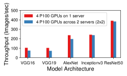
Many apps, many preference patterns: ML cluster users today train a variety of ML apps across domains like computer vision, NLP and speech recognition. These models have significantly different model architectures, and more importantly, different placement preferences arising from different computation, communication needs. For example, as shown in Figure 5, VGG16 has a strict machine-local task placement preference while Resnet50 does not. This preference inherently stems from the fact that VGG-like architectures have very large number of parameters and incur greater overheads for updating gradients over the network.

Figure 5: Effect of GPU resource allocation on job throughput.

We use examples to show the effect of placement on DRF’s allocation strategy. Similar examples and conclusions apply for the LAS allocation scheme.

Ignoring placement affects SI: example: Consider the Instance 1 in Figure 6. In this example, there are two placement sensitive ML apps - $A_{1}$ reflecting VGG16, and $A_{2}$ reflecting VGG19. Each ML app has just one job in it with $4$ tasks and the cluster has two $4$ GPU machines. As shown above, given the same number of GPUs both apps prefer GPUs to be in the same server than spread across servers.

For this example, DRF [8] equalizes the dominant resource share of both the apps under resource constraints and allocates $4$ GPUs to each ML app. In Instance 1 of Figure 6 we show an example of a valid DRF allocation. Both apps get the same type of placement with GPUs spread across servers. This allocation violates SI for both apps as their performance would be better if each app just had its own dedicated server.

Ignoring placement affects PE, EF: example: Consider Instance 2 in Figure 6 with two apps - $A_{1}$ (Inceptionv3) which is not placement sensitive and $A_{2}$ (VGG16) which is placement sensitive. Each app has one job with four tasks and and the cluster has two machines: one $4$ GPU and two $2$ GPU.

Now consider the allocation in Instance 2, where $A_{1}$ is allocated on the $4$ GPU machine whereas $A_{2}$ is allocated across the 2 GPU machines. This allocation violates EF, because $A_{2}$ would prefer $A_{1}$’s allocation. It also violates PE because swapping the two apps’ allocation would improve $A_{2}$’s performance without hurting $A_{1}$.

Figure 6: By ignoring placement preference, DRF violates sharing incentive.

In fact, we can formally show that:

Theorem 3.1. Existing fair schemes (DRF, LAS) ignore placement preferences and violate SI, PE, EF for ML apps.

Proof Refer to Appendix.

In summary, existing schemes fail to provide fair sharing guarantees as they are unaware of ML app characteristics. Instantaneous fair schemes such as DRF fail to account for long task durations. While least-attained service schemes overcome that limitation, neither approach’s input encodes placement preferences. Correspondingly, the fairness metrics used - i.e., dominant resource share (DRF) or attained service (LAS) - do not capture placement preferences.

This motivates the need for a new placement-aware fairness metric, and corresponding scheduling discipline. Our observations about ML task durations imply that, like LAS, our fair allocation discipline should not depend on rapid task completions, but instead should operate over longer time scales.

3.2 Metric: Finish-Time Fairness

We propose a new metric called as finish-time fairness, $\rho$. $\rho=\frac{T_{sh}}{T_{id}}$.

$T_{id}$ is the independent finish-time and $T_{sh}$ is the shared finish-time. $T_{sh}$ is the finish-time of the app in the shared cluster and it encompasses the slowdown due to the placement and any queuing delays that an app experiences in getting scheduled in the shared cluster. The worse the placement the higher is the value of $T_{sh}$. $T_{id}$, is the finish-time of the ML app in its own independent and exclusive $\frac{1}{N}$ share of the cluster. Given the above definition, sharing incentive for an ML app can be attained if $\rho\leq 1$.

To ensure this, it is necessary for the allocation mechanism to estimate the values of $\rho$ for different GPU allocations. Given the difficulty in predicting how various apps will react to different allocations, it is intractable for the scheduling engine to predict or determine the values of $\rho$.

Thus we propose a new wider interface between the app and the allocation engine that can allow the app to express a preference for each allocation. We propose that apps can encode this information as a table. In Table 1, each column has a permutation of a potential GPU allocation and the estimate of $\rho$ on receiving this allocation. We next describe how the scheduling engine can use this to provide fair allocations.

$\overrightarrow{G}$	$[0,0]$	$[0,1]=[1,0]$	$[1,1]$
$\rho$	$\rho_{old}$	$\frac{200}{400}=\frac{1}{2}$	$\frac{100}{400}=\frac{1}{4}$

Table 1: Example table of bids sent from apps to the scheduler

3.3 Mechanism: Partial Allocation Auctions

1:Applications {$\textit{A}_{i}$} $\triangleright$ set of apps

2:Bids {$\mathbb{\rho}_{i}(.)$} $\triangleright$ valuation function for each app $i$

3:Resources $\overrightarrow{R}$ $\triangleright$ resource set available for auction

4:Resource Allocations {$\overrightarrow{G}_{i}$} $\triangleright$ resource allocation for each app $i$

5:

6:procedure auction({$\textit{A}_{i}$}, {$\mathbb{\rho}_{i}(.)$}, $\overrightarrow{R}$)

7:    $\overrightarrow{G}_{i,pf}$ = arg max $\prod_{i}1/\mathbb{\rho}_{i}(\overrightarrow{G_{i}})$ $\triangleright$ proportional fair (pf) allocation per app $i$

8:    $\overrightarrow{G}^{-i}_{j,pf}$ = arg max $\prod_{j!=i}1/\mathbb{\rho}_{j}(\overrightarrow{G_{j}})$ $\triangleright$ pf allocation per app $j$ without app $i$

9:    $c_{i}$ = $\frac{\prod_{j!=i}1/\mathbb{\rho}_{j}(\overrightarrow{G}_{j,pf})}{\prod_{j!=i}1/\mathbb{\rho}_{j}(\overrightarrow{G}^{-i}_{j,pf})}$

10:    $\overrightarrow{G_{i}}$ = $c_{i}$ * $\overrightarrow{G}_{i,pf}$ $\triangleright$ allocation per app $i$

11:    $\overrightarrow{L}$ = $\sum_{i}$ $1-c_{i}$ * $\overrightarrow{G}_{i,pf}$ $\triangleright$ aggregate leftover resource

12:    return {$\overrightarrow{G_{i}}$}, $\overrightarrow{L}$

13:end procedure

14:procedure roundByRoundAuctions({$\textit{A}_{i}$}, {$\mathbb{\rho}_{i}(.)$})

15:    while True do

16:       onResourceAvailableEvent $\vec{R^{\prime}}$:

17:       {$A_{i}^{sort}$} = sort({${A_{i}}$}) on $\rho_{i}^{current}$

18:       {$A_{i}^{filter}$} = get top $1-f$ fraction of apps from {$A_{sort}$}

19:       {$\rho_{i}^{filter}(.)$} = get updated $\rho(.)$ from apps in {$A_{i}^{filter}$}

20:       {$\overrightarrow{G_{i}^{filter}}$}, $\overrightarrow{L}$ = auction({$A_{i}^{filter}$}, {$\rho_{i}^{filter}(.)$}, $\vec{R^{\prime}}$)

21:       {$A_{i}^{unfilter}$} = $\{A_{i}\}-\{A_{i}^{filter}\}$

22:       allocate $\overrightarrow{L}$ to {$A_{i}^{unfilter}$} at random

23:    end while

24:end procedure

Pseudocode 1 Finish-Time Fair Policy

The finish-time fairness $\rho_{i}(.)$ for an ML app $A_{i}$ is a function of the GPU allocation $\vec{G_{i}}$ that it receives. The allocation policy takes these $\rho_{i}(.)$’s as inputs and outputs allocations $\vec{G_{i}}$.

Intuitively the scheduling engine would pick the apps that can most benefit from an allocation and assign resources to that app. In other words allocations which can decrease an app’s $\rho_{i}$ will be preferred. However, one of the main challenges in a two level design where apps submit their respective $\rho_{i}$’s is that apps could potentially return false information to boost the chances that they receive a particular allocation. Our conversations with cluster operators indicate that apps request for more resources than required and the require monitoring (“We also monitor the usage. If they don’t use it, we reclaim it and pass it on to the next approved project”). Thus a simple scheme like sorting the apps based on their reported $\rho$ values would fail to provide another key property, namely, strategy proofness (SP).

To address this challenge, we propose to use auctions in Themis. We begin by describing a simple mechanism that runs a single-round auction and then extend to a round-by-round mechanism that also considers online updates.

3.3.1 One-Shot Auction

Details of the inputs necessary to run the auction are given first, followed by how the auction works given these inputs.

Inputs: Resources and Bids. $\vec{R}$ represents the total GPU resources to be auctioned, where each element is $1$ and the number of dimensions is the number of GPUs to be auctioned.

Each ML app bids for these resources. The bid for each ML app consists of the estimated finish-time fair metric ($\rho_{i}$) values for several different GPU allocations ($\vec{G}_{i}$). Each element in $\vec{G}_{i}$ can be $\{0,1\}$. A set bit implies that GPU is allocated to the app. Example of a bid can be seen in Table 1.

Auction Overview. To ensure that the auction can provide strategy proofness, we propose using a partial allocation auction (PA) mechanism [5]. Partial allocation auctions have been shown to incentivize truth telling and are an appropriate fit for modeling subsets of indivisible goods to be auctioned across apps. Pseudocode 1, line $5$ shows the PA mechanism. There are two aspects to auctions that are described next.

1. Initial allocation. PA starts by calculating an intrinsically proportionally-fair allocation $\vec{G_{i,pf}}$ for each app $A_{i}$ by maximizing the product of the valuation functions i.e. the finish-time fair metric values for all apps (Pseudocode 1, line $6$). Such an allocation ensures that it is not possible to increase the allocation of an app without decreasing the allocation of at least another app (satisfying PE [5]).

2. Incentivizing Truth Telling. To induce truthful reporting of the bids, the PA mechanism allocates app $A_{i}$ only a fraction $c_{i}<1$ of $A_{i}$’s proportional fair allocation $\vec{G_{i,pf}}$, and takes $1-c_{i}$ as a hidden payment (Pseudocode 1, line $9$). The $c_{i}$ is directly proportional to the decrease in collective valuation of the other bidding apps in a market with and without app $A_{i}$ (Pseudocode 1, line $8$). This yields the final allocation $\vec{G_{i}}$ for app $A_{i}$ (Pseudocode 1, line $9$).

Note that the final result, $\vec{G_{i}}$ is not a market-clearing allocation and there could be unallocated GPUs $\vec{L}$ that are leftover from hidden payments. Hence, PA is not work-conserving. Thus, while the one-shot auction provides a number of properties related to fair sharing it does not ensure SI is met.

Theorem 3.2. The one-shot partial allocation auction guarantees SP, PE and EF, but does not provide SI.

Proof Refer to Appendix.

The intuitive reason for this is that the partial allocation mechanism does not explicitly ensure that $\rho\leq 1$ across apps. To address this we next look at multi-round auctions that can maximize sharing incentive for ML apps.

3.3.2 Multi-round auctions

To maximize sharing incentive and to ensure work conservation, our goal is to ensure $\rho\leq 1$ for as many apps as possible. We do this using three key ideas described below.

Round-by-Round Auctions: With round-by-round auctions, the outcome of an allocation from an auction is binding only for a lease duration. At the end of this lease, the freed GPUs are re-auctioned. This also handles the online case as any auction is triggered on a resource available event. This takes care of app failures and arrivals, as well as cluster reconfigurations.

At the beginning of each round of auction, the policy solicits updated valuation functions $\rho(.)$ from the apps. The estimated work and the placement preferences for the case of ML apps are typically time varying. This also makes our policy adaptive to such changes.

Round-by-Round Filtering: To maximize the number of apps with $\rho\leq 1$, at the beginning of each round of auctions we filter the $1-f$ fraction of total active apps with the greatest values of current estimate of their finish-time fair metric $\rho$. Here, $f\in(0,1)$ is a system-wide parameter.

This has the effect of restricting the auctions to the apps that are at risk of not meeting SI. Also, this restricts the auction to a smaller set of apps which reduces contention for resources and hence results in smaller hidden payments. It also makes the auction computationally tractable.

Over the course of many rounds, filtering maximizes the number of apps that have SI. Consider a far-from-fair app $i$ that lost an auction round. It will appear in future rounds with much greater likelihood relative to another less far-from-fair app $k$ that won the auction round. This is because, the winning app $k$ was allocated resources; as a result, it will see its $\rho$ improve over time; thus, it will eventually not appear in the fraction $1-f$ of not-so-fairly-treated apps that participate in future rounds. In contrast, $i$’s $\rho$ will increase due to the waiting time, and thus it will continue to appear in future rounds. Further an app that loses multiple rounds will eventually lose its lease on all resources and make no further progress, causing its $\rho$ to become unbounded. The next auction round the app participates in will likely see the app’s bid winning, because any non-zero GPU allocation to that app will lead to a huge improvement in the app’s valuation.

As $f\rightarrow 1$, our policy provides greater guarantee on SI. However, this increase in SI comes at the cost of efficiency. This is because $f\rightarrow 1$ restricts the set of apps to which available GPUs will be allocated; with $f\rightarrow 0$ available GPUs can be allocated to apps that benefit most from better placement, which improves efficiency at the risk of violating SI.

Leftover Allocation: At the end of each round we have leftover GPUs due to hidden payments. We allocate these GPUs at random to the apps that did not participate in the auction in this round. Thus our overall scheme is work-conserving.

Overall, we prove that:

Theorem 3.3. Round-by-round auctions preserve the PE, EF and SP properties of partial auctions and maximize SI.

Proof. Refer to Appendix.

To summarize, in Themis we propose a new finish-time fairness metric that captures fairness for long-running, placement sensitive ML apps. To perform allocations, we propose using a multi-round partial allocation auction that incentivizes truth telling and provides pareto efficient, envy free allocations. By filtering the apps considered in the auction, we maximize sharing incentive and hence satisfy all the properties necessary for fair sharing among ML applications.

4 System Design

We first list design requirements for an ML cluster scheduler taking into account the fairness metric and auction mechanism described in Section 3, and the implications for the Themis scheduler architecture. Then, we discuss the API between the scheduler and the hyper-parameter optimizers.

4.1 Design Requirements

Separation of visibility and allocation of resources. Core to our partial allocation mechanism is the abstraction of making available resources visible to a number of apps but allocating each resource exclusively to a single app. As we argue below, existing scheduling architectures couple these concerns and thus necessitate the design of a new scheduler.

Integration with hyper-parameter tuning systems. Hyper-parameter optimization systems such as Hyperband [22], Hyperdrive [30] have their own schedulers that decide the resource allocation and execution schedule for the jobs within those apps. We refer to these as app-schedulers. One of our goals in Themis is to integrate with these systems with minimal modifications to app-schedulers.

These two requirements guide our design of a new two-level semi-optimistic scheduler and a set of corresponding abstractions to support hyper-parameter tuning systems.

4.2 Themis Scheduler Architecture

Existing scheduler architectures are either pessimistic or fully optimistic and both these approaches are not suitable for realizing multi-round auctions. We first describe their shortcomings and then describe our proposed architecture.

4.2.1 Need for a new scheduling architecture

Two-level pessimistic schedulers like Mesos [17] enforce pessimistic concurrency control. This means that visibility and allocation go hand-in-hand at the granularity of a single app. There is restricted single-app visibility as available resources are partitioned by a mechanism internal to the lower-level (i.e., cross-app) scheduler and offered only to a single app at a time. The tight coupling of visibility and allocation makes it infeasible to realize round-by-round auctions where resources need to be visible to many apps but allocated to just one app.

Shared-state fully optimistic schedulers like Omega [31] enforce fully optimistic concurrency control. This means that visibility and allocation go hand-in-hand at the granularity of multiple apps. There is full multi-app visibility as all cluster resources and their state is made visible to all apps. Also, all apps contend for resources and resource allocation decisions are made by multiple apps at the same time using transactions. This coupling of visibility and allocation in a makes it hard to realize a global policy like finish-time fairness and also leads to expensive conflict resolution (needed when multiple apps contend for the same resource) when the cluster is highly contented, which is typically the case in shared GPU clusters.

Thus, the properties required by multi-round auctions, i.e., multi-app resource visibility and single-app resource allocation granularity, makes existing architectures ineffective.

4.2.2 Two-Level Semi-Optimistic Scheduling

Figure 7: Themis Design. (a) Sequence of events in Themis - starts with a resource available event and ends with resource allocations. (b) Shows a typical bid valuation table an App submits to Arbiter. Each row has a subset of the complete resource allocation and the improved value of $\rho_{new}$.

The two-levels in our scheduling architecture comprise of multiple app-schedulers and a cross-app scheduler that we call the arbiter. The Arbiter has our scheduling logic. The top level per-app schedulers are minimally modified to interact with the Arbiter. Figure 7 shows our architecture.

Each GPU in a Themis-managed cluster has a lease associated with it. The lease decides the duration of ownership of the GPU for an app. When a lease expires, the resource is made available for allocation. Themis’s Arbiter pools available resources and runs a round of the auctions described earlier. During each such round, the resource allocation proceeds in 5 steps spanning 2 phases (shown in Figure 7):

The first phase, called the visibility phase, spans steps 1–3.

The Arbiter asks all apps for current finish-time fair metric estimates. The Arbiter initiates auctions, and makes the same non-binding resource-offer of the available resources to to a fraction $f\in[0,1]$ of ML apps with worst finish-time fair metrics (according to round-by-round filtering described earlier). To minimize changes in the ML app scheduler to participate in auctions, Themis introduces an Agent that is co-located with each ML app scheduler. The Agent serves as an intermediary between the ML app and the Arbiter. The apps examine the resource offer in parallel. Each app’s Agent then replies with a single bid that contains preferences for desired resource allocations.

The second phase, allocation phase, spans steps 4–5. The Arbiter, upon receiving all the bids for this round, picks winning bids according to previously described partial allocation algorithm and leftover allocation scheme. It then notifies each Agent of its winning allocation (if any). The Agent propagates the allocation to the ML app scheduler, which can then decide the allocation among constituent jobs.

In sum, the two phase resource allocation means that our scheduler enforces semi-optimistic concurrency control. Similar to fully optimistic concurrency control, there is multi-app visibility as the cross-app scheduler offers resources to multiple apps concurrently. At the same time, similar to pessimistic concurrency control, the resource allocations are conflict-free guaranteeing exclusive access of a resource to every app.

To enable preparation of bids in step , Themis implements a narrow API from the ML app scheduler to the Agent that enables propagation of app-specific information. An Agent’s bid contains a valuation function ($\rho(.)$) that provides, for each resource subset, an estimate of the finish-time fair metric the app will achieve with the allocation of the resource subset. We describe how this is calculated next.

4.3 Agent and AppScheduler Interaction

An Agent co-resides with an app to aid participation in auctions. We now describe how Agents prepare bids based on inputs provided by apps, the API between an Agent and its app, and how Agents integrate with current hyper-parameter optimization schedulers.

4.3.1 Single-Job ML Apps

For ease of explanation, we first start with the simple case of an ML app that has just one ML training job which can use at most $job\_demand_{max}$ GPUs. We first look at calculation of the finish-time fair metric, $\rho$. We then look at a multi-job app example so as to better understand the various steps and interfaces in our system involved in a multi-round auction.

Calculating $\rho(\overrightarrow{G})$. Equation 1 shows the steps for calculating $\rho$ for a single job given a GPU allocation of $\overrightarrow{G}$ in a cluster $C$ with $R_{C}$ GPUs. When calculating $\rho$ we assume that the allocation $\overrightarrow{G}$ is binding till job completion.

$$\begin{split}\rho(\overrightarrow{G})&=T_{sh}(\overrightarrow{G})/T_{id}\\ T_{sh}&=T_{current}-T_{start}+\\ &iter\_left*iter\_time(\overrightarrow{G})\\ T_{id}&=T_{cluster}*N_{avg}\\ iter\_time(\overrightarrow{G})&=\frac{iter\_time\_serial*\mathcal{S}(\overrightarrow{G})}{min(||\overrightarrow{G}||_{1},job\_demand_{max})}\\ T_{cluster}&=\frac{iter\_total*iter\_serial\_time}{min(R_{C},job\_demand_{max})}\end{split}$$ (1)

$T_{sh}$ is the shared finish-time and is a function of the allocation $\overrightarrow{G}$ that the job receives. For the single job case, it has two terms. First, is the time elapsed ($=T_{current}-T_{start}$). Time elapsed also captures any queuing delays or starvation time. Second, is the time to execute remaining iterations which is the product of the number of iterations left ($iter\_left$) and the iteration time ($iter\_time(\overrightarrow{G})$). $iter\_time(\overrightarrow{G})$ depends on the allocation received. Here, we consider the common-case of the ML training job executing synchronous SGD. In synchronous SGD, the work in an iteration can be parallelized across multiple workers. Assuming linear speedup, this means that the iteration time is the serial iteration time ($iter\_time\_serial$) reduced by a factor of the number of GPUs in the allocation, $||\overrightarrow{G}||_{1}$ or $job\_demand_{max}$ whichever is lesser. However, the linear speedup assumption is not true in the common case as network overheads are involved. We capture this via a slowdown penalty, $\mathcal{S}(\overrightarrow{G})$, which depends on the placement of the GPUs in the allocation. Values for $\mathcal{S}(\overrightarrow{G})$ can typically be obtained by profiling the job offline for a few iterations. The slowdown is captured as a multiplicative factor, $\mathcal{S}(\overrightarrow{G})\geq 1$, by which $T_{sh}$ is increased.

$T_{id}$ is the estimated finish-time in an independent $\frac{1}{N_{avg}}$ cluster. $N_{avg}$ is the average contention in the cluster and is the weighed average of the number of other apps in the system during the lifetime of the app. We approximate this as the finish-time of the app in the whole cluster, $T_{cluster}$ divided by the average contention. $T_{cluster}$ assumes linear speedup when the app executes with all the cluster resources $R_{C}$ or maximum app demand whichever is lesser. It also assumes no slowdown. Thus, it is approximated as $\frac{iter\_total*iter\_serial\_time}{min(R_{C},job\_demand_{max})}$.

4.3.2 Generalizing to Mutiple-Job ML Apps

ML app schedulers for hyper-parameter optimization systems typically go from aggressive exploration of hyper-parameters to aggressive exploitation of best hyper-parameters. While there are a number of different algorithms for choosing the best hyper-parameters [22, 3] to run, we focus on early stopping criteria as this affects the finish time of ML apps.

As described in prior work [9], automatic stopping algorithms can be divided into two categories: Successive Halving and Performance Curve Stopping. We next discuss how to compute $T_{sh}$ for each case.

Successive Halving refers to schemes which start with a total time or iteration budget $B$ and apportion that budget by periodically stopping jobs that are not promising. For example, if we start with $n$ hyper parameter options, then each one is submitted as a job with a demand of $1$ GPU for a fixed number of iterations $I$. After $I$ iterations, only the best $\frac{n}{2}$ ML training jobs are retained and assigned a maximum demand of $2$ GPUs for the same number of iterations $I$. This continues until we are left with $1$ job with a maximum demand of $n$ GPUs. Thus there are a total of $log_{2}n$ phases in Successive Halving. This scheme is used in Hyperband [22] and Google Vizier [9].

We next describe how to compute the $T_{sh}$ and $T_{id}$ for successive halving. We assume that the given allocation $\overrightarrow{G}$ lasts till app completion and the total time can be computed by adding up the time the app spends for each phase. Consider the case of phase $i$ which has $J=\frac{n}{2^{i-1}}$ jobs. Equation 2 shows the calculation of $T_{sh(i)}$, the shared finish time of the phase. We assume a separation of concerns where the hyper-parameter optimizer can determine the optimal allocation of GPUs within a phase and thus estimate the value of $\mathcal{S}(\overrightarrow{G_{j}})$. Along with $iter\_left$, $serial\_iter\_time$, the Agent can now estimate $T_{sh(j)}$ for each job in the phase. We mark the phase as finished when the slowest or last job in the app finishes the phase ($max_{j}$). Then the shared finish time for the app is the sum of the finish times of all constituent phases.

To estimate the ideal finish-time we compute the total time to execute the app on the full cluster. We estimate this using the budget $B$ which represents the aggregate work to be done and, as before, we assume linear speedup to the maximum number of GPUs the app can use $app\_demand_{max}$.

$$\begin{split}T_{sh(i)}&=max_{j}\{T(\overrightarrow{G_{j}})\}\\ T_{sh}&=\sum_{i}T_{sh(i)}\\ T_{cluster}&=\frac{B}{min(R_{C},app\_demand_{max})}\\ T_{id}&=T_{cluster}*N_{avg}\end{split}$$ (2)

The Agent generates $\rho$ using the above procedure for all possible subsets of $\{\overrightarrow{G}\}$ and produced a bid table similar to the one shown in Table 1 before. The API between the Agent and hyper-parameter optimizer is shown in Figure 8 and captures the functions that need to implemented by the hyper-parameter optimizer.

Performance Curve Stopping refers to schemes where the convergence curve of a job is extrapolated to determine which jobs are more promising. This scheme is used by Hyperdrive [30] and Google Vizier [9]. Computing $T_{sh}$ proceeds by calculating the finish time for each job that is currently running by estimating the iteration at which the job will be terminated (Thus $T_{sh}$ is determined by the job that finishes last). As before, we assume that the given allocation $\overrightarrow{G}$ lasts till app completion. Since the estimations are usually probabilistic (i.e. the iterations at which the job will converge has an error bar), we over-estimate and use the most optimistic convergence curve that results in the maximum forecasted completion time for that job. As the job progresses, the estimates of the convergence curve get more accurate and improving the estimated finish time $T_{sh}$. The API implemented by the hyper-parameter optimizer is simpler and only involves getting a list of running jobs as shown in Figure 8.

We next present an end-to-end example of a multi-job app showing our mechanism in action.

4.3.3 End-to-end Example.

We now run through a simple example that exercises the various aspects of our API and the interfaces involved.

Consider a $16$ GPU cluster and an ML app that has $4$ ML jobs and uses successive halving, running along with 3 other ML apps in the same cluster. Each job in the app is tuning a different hyper-parameter and the serial time taken per iteration for the jobs are $80,100,100,120$ seconds respectively. The total budget for the app is to $10,000$ seconds of GPU time and we assume the $job\_demand_{max}$ is $8$ GPUs and $\mathcal{S}(\overrightarrow{G})=1$.

Given we start with $4$ ML jobs, the hyper-parameter optimizer divides this into 3 phases each having $4,2,1$ jobs, resply. To evenly divide the budget across the phases, the hyper-parameter optimizer budgets $\approx 8,16,36$ iterations in each phase. First we calculate the $T_{id}$ by considering the budget, total cluster size, and cluster contention as: $\frac{10000\times 4}{16}=2500$s.

Next we consider the computation of $T_{sh}$ assuming that $16$ GPUs are offered by the arbiter. The agent now computes the bid for each subset of GPUs offered. Consider the case with $2$ GPUs. In this case in the first phase we have $4$ jobs which are serialized to run $2$ at a time. This leads to $T_{sh(1)}=(120\times 8)+(80\times 8)=1600$ seconds. (Assume two 100s jobs run serially on one GPU, and the 80 and 120s jobs run serially on the other. $T_{sh}$ is the time when the last job finishes.)

When we consider the next stage the hyper-parameter optimizer currently does not know which jobs will be chosen for termination. We use the median job (in terms of per-iteration time) to estimate $T_{sh(i)}$ for future phases. Thus, in the second phase we have $2$ jobs so we run one job on each GPU each of which we assume to take the median $100$ seconds per iteration leading to $T_{sh(2)}=(100\times 16)=1600$ seconds. Finally for the last phase we have $1$ job that uses $2$ GPUs and runs for $36$ iterations leading to $T_{sh(3)}=\frac{(100\times 36)}{2}=1800$ (again, the “median” jobs takes 100s per iteration). Thus $T_{sh}=1600+1600+1800=5000$ seconds, making $\rho=\frac{5000}{2500}=2$. Note that since placement did not matter here we considered any $2$ GPUs being used. Similarly ignoring placement, the bids for the other allocations are shown in Table 2.

We highlight a few more points about our example above. If the jobs that are chosen for the next phase do not match the median iteration time then the estimates are revised in the next round of the auction. For example if the jobs that are chosen for the next round have iteration time $120,100$ then the above bid will be updated with $T_{sh(2)}=(120\times 16)=3200$ and $T_{sh(3)}=\frac{(120\times 36)}{2}=2160$. Further we also see that the $job\_demand_{max}=8$ means that the $\rho$ value for $16$ GPUs does not linearly decrease from that of $8$ GPUs.

class JobInfo(int itersRemaining,
              float avgTimePerIter,
              float localitySensitivity);
// Successive Halving
List<JobInfo> getJobsInPhase(int phase,
                             List<Int> gpuAlloc);
int getNumPhases();
// Performance Curve
List<JobInfo> getJobsRemaining(List<Int> gpuAlloc);
    

Figure 8: API between Agent and hyperparameter optimizer

$||\overrightarrow{G}||_{1}$	$0$	$1$	$2$	$4$	$8$	$16$
$\rho$	$\rho_{old}$	$4$	$2$	$1$	$0.5$	$0.34$

Table 2: Example of bids submitted by Agent

5 Implementation

We implement Themis on top of a recent release of Apache Hadoop YARN [1] (version $3.2.0$) which includes, Submarine [2], a new framework for running ML training jobs atop YARN. We modify the Submarine client to support submitting a group of ML training jobs as required by hyper-parameter exploration apps. Once an app is submitted, it is managed by a Submarine Application Master (AM) and we make changes to the Submarine AM to implement the ML app scheduler (we use Hyperband [22]) and our Agent.

To prepare accurate bids, we implement a profiler in the AM that parses TensorFlow logs, and tracks iteration times and loss values for all the jobs in an app. The allocation of a job changes over time and iteration times are used to accurately estimate the placement sensitivity ($\mathcal{S}$) from different GPU placements. Loss values are used in our Hyperband implementation to determine early stopping. Themis’s Arbiter is implemented as a separate module in YARN RM. We add gRPC-based interfaces between the Agent and the Arbiter to enable offers, bids, and final winning allocations. Further, the Arbiter tracks GPU leases to offer reclaimed GPUs as a part of the offers.

All the jobs we use in our evaluation are TensorFlow programs with configurable hyper-parameters. To handle allocation changes at runtime, the programs checkpoint model parameters to HDFS every few iterations. After a change in allocation, they resume from the most recent checkpoint.

6 Evaluation

We evaluate Themis on a $64$ GPU cluster and also use a event-driven simulator to model a larger $256$ GPU cluster. We compare against other state-of-the-art ML schedulers. Our evaluation shows the following key highlights -

• Themis is better than other schemes on finish-time fairness while also offering better cluster efficiency (Figure 9- 10). These experiments are done in our testbed.

• Themis’s benefits compared to other schemes improve with increasing fraction of placement sensitive apps and increasing contention in the cluster, and these improvements hold even with errors – random and strategic – in finish-time fair metric estimations (Figure 12 - 15).

• Themis enables a trade-off between finish-time fairness in the long-term and placement efficiency in the short-term. Sensitivity analysis (Figure 16) using simulations show that $f=0.8$ and a lease time of $10$ minutes gives maximum fairness while also utilizing the cluster efficiently.

6.1 Experimental Setup

Testbed Setup. Our testbed is a $64$ GPU, $20$ machine cluster on Microsoft Azure [24]. We use NC-series instances. We have $8$ NC12-series instances each with $2$ Tesla K80 GPUs and $12$ NC24-series instances each with $4$ Tesla K80 GPUs.

Simulator. We develop an event-based simulator to evaluate Themis at large scale. The simulator assumes that estimates of the loss function curves for jobs are known ahead of time so as to predict the total number of iterations for the job. Unless stated otherwise, all simulations are done on a heterogeneous $256$ GPU cluster. Our simulator assumes a $4$-level hierarchical locality model for GPU placements. Individual GPUs fit onto slots on machines occupying different cluster racks.

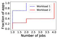
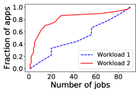
Workload. We experiment with $2$ different traces that have different workload characteristics in both the simulator and the testbed - (i) Workload 1. A publicly available trace of DNN training workloads at Microsoft [20, 25]. We scale-down the trace, using a two week snapshot and focusing on subset of jobs from the trace that correspond to hyper-parameter exploration jobs triggered by Hyperdrive. (ii) Workload 2. We use the app arrival times from Workload 1, generate jobs per app using the successive halving pattern characteristic of the Hyperband algorithm [22], and increase the number of tasks per job compared to Workload 1. The distribution of number of tasks per job and number of jobs per app for the two workloads is shown in the Appendix A (Figure 17).

Baselines. We compare Themis against four state-of-the-art ML schedulers - Gandiva [40], Tiresias [13], Optimus [28], and SLAQ [43]; these represent the best possible baselines for maximizing efficiency, maximizing fairness, minimizing average app completion time, and maximizing aggregate model quality, respectively. We implement these baselines in our testbed as well as the simulator as described below:

Ideal Efficiency Baseline - Gandiva. Gandiva improves cluster utilization by packing jobs on as few machines as possible. In our implementation, Gandiva introspectively profiles ML job execution to infer placement preferences and migrates jobs to better meet these placement preferences. On any resource availability, all apps report their placement preferences and we allocate resources in a greedy highest preference first manner which has the effect of maximizing the average placement preference across apps. We do not model time-slicing and packing of GPUs as these system-level techniques can be integrated with Themis as well and would benefit Gandiva and Themis to equal extents.

Ideal Fairness Baseline - Tiresias. Tiresias defines a new service metric for ML jobs – the aggregate GPU-time allocated to each job – and allocates resources using the Least Attained Service (LAS) policy so that all jobs obtain equal service over time. In our implementation, on any resource availability, all apps report their service metric and we allocate the resource to apps that have the least GPU service. We do not implement the Gittin’s index policy from Tiresias as it enables a trade-off between service-based fairness and average app completion time. Instead, we use a different baseline for average app completion time.

Ideal Average App Completion Time Baseline - Optimus. Optimus proposes the Shortest Remaining Time First (SRTF) policy for ML jobs. In our implementation, on any resource availability, all apps report their remaining time with allocations from the available resources and we allocate these resources using the SRTF policy.

Ideal Aggregate Model Quality - SLAQ. SLAQ proposes a greedy scheme for improving aggregate model quality across all jobs. In our implementation, on any resource availability event, all apps report the decrease in loss value with allocations from the available resources and we allocate these resources in a greedy highest loss first manner.

(a)

(b)

Figure 9: [Testbed] Comparison of finish-time fairness across schedulers

Metrics. We use a variety of metrics to evaluate Themis.

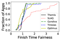
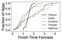
(i) Finish-time fairness: We evaluate the fairness of schemes by looking at the finish-time fair metric ($\rho$) distribution and the maximum value across apps. A tighter distribution and a lower value of maximum value of $\rho$ across apps indicate higher fairness. (ii) GPU Time: We use GPU Time as a measure of how efficiently the cluster is utilized. For two scheduling schemes $S_{1}$ and $S_{2}$ that have GPU times $G_{1}$ and $G_{2}$ for executing the same amount of work, $S_{1}$ utilizes the cluster more efficiently than $S_{2}$ if $G_{1}<G_{2}$. (iii) Placement Score: We give each allocation a placement score ($\leq 1$). This is inversely proportional to slowdown, $\mathcal{S}$, that app experiences due to this allocation. The slowdown is dependent on the ML app properties and the network interconnects between the allocated GPUs. A placement score of $1.0$ is desirable for as many apps as possible.

6.2 Macrobenchmarks

In our testbed, we evaluate Themis against all baselines on all the workloads. We set the fairness knob value $f$ as $0.8$ and lease as $10$ minutes, which is informed by our sensitivity analysis results in Section 6.4.

Figure 9 shows the distribution of finish-time fairness metric, $\rho$, across apps for Themis and all the baselines. We see that Themis has a narrower distribution for the $\rho$ values which means that Themis comes closest to giving all jobs an equal sharing incentive. Also, Themis has the maximum $\rho$ value $2.2X$, $2.25X$, $1.75X$, and $3.25X$ better than Gandiva, Tiresias, Optimus, and SLAQ, respectively. Figure 10 shows a comparison of the efficiency in terms of the aggregate GPU time to execute the complete workload. Workload 1 has similar efficiency across Themis and the baselines as all jobs are either $1$ or $2$ GPU jobs and almost all allocations, irrespective of the scheme, end up as efficient. With workload 2, Themis betters Gandiva by ~4.8% and outperforms SLAQ by ~250%. This improvement is because Themis leads to global optimality in placement-driven packing due to the auction abstraction. Gandiva in contrast takes greedy locally optimal decisions.

6.2.1 Sources of Improvement

In this section, we deep-dive into the reasons behind the wins in fairness and cluster efficiency in Themis.

Job Type	GPU Time	# GPUs	$\rho_{\textsc{Themis}{}}$	$\rho_{Tiresias}$
Long Job	~580 mins	4	~1	~0.9
Short Job	~83 mins	2	~1.2	~1.9

Table 3: [Testbed] Details of 2 jobs to understand the benefits of Themis

(a)

(b)

Figure 10: [Testbed] Comparison of total GPU times across schemes. Lower GPU time indicates better utilization of the GPU cluster

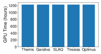
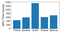
Table 3 compares the finish-time fair metric value for a pair of short- and long-lived apps from our testbed run for Themis and Tiresias. Themis offers better sharing incentive for both the short and long apps. Themis induces altruistic behavior in long apps. We attribute this to our choice of $\rho$ metric. With less than ideal allocations, even though long apps see an increase in $T_{sh}$, their $\rho$ values do not increase drastically because of a higher $T_{id}$ value in the denominator. Whereas, shorter apps see a much more drastic degradation, and our round-by-round filtering of farthest-from-finish-time fairness apps causes shorter apps to participate in auctions more often. Tiresias offers poor sharing incentive for short apps as it treats short- and long-apps as the same. This only worsens the sharing incentive for short apps.

Figure 11: Testbed] CDF of placement scores across schemes

Figure 12: [Testbed] Impact of contention on finish-time fairness

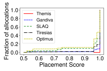
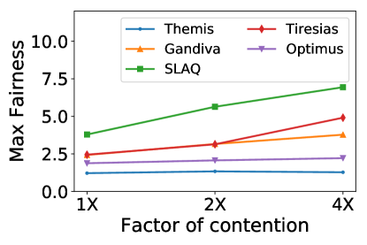
Figure 12 shows the distribution of placement scores for all the schedulers. Themis gives the best placement scores (closer to 1.0 is better) in workload 2, with Gandiva coming closest. Workload 1 has jobs with very low GPU demand and almost all allocations have a placement score of 1 irrespective of the scheme. Tiresias, SLAQ, and Optimus are poor as they are agnostic of placement preferences. Gandiva performs better but is not as efficient because of greedy local packing.

6.2.2 Effect of Contention

In this section, we analyze the effect of contention on finish-time fairness. We decrease the size of the cluster to half and quarter the original size to induce a contention of 2$X$ and 4$X$ respectively. Figure 12 shows the change in max value of $\rho$ as the contention changes with workload 1. Themis is the only scheme that maintains sharing incentive even in high contention scenarios. Optimus comes close as it preferably allocates resources to shorter apps. This behavior is similar to that in Themis. Themis induces altruistic shedding of resources by longer apps (Section 6.2.1), giving shorter apps a preference in allocations during higher contention.

6.2.3 Systems Overheads

From our profiling of the experiments above, we find that each Agent spends 29 (334) milliseconds to compute bids at the median (95-%). The 95 percentile is high because enumeration of possible bids needs to traverse a larger search space when the number of resources up for auction is high.

The Arbiter uses Gurobi [14] to compute partial allocation of resources to apps based on bids. This computation takes  354 (1398) milliseconds at the median (95-%ile). The high tail is once again observed when both the number of offered resources and the number of apps bidding are high. However, the time is small relative to lease time. The network overhead for communication between the Arbiter and individual apps is negligible since we use the existing mechanisms used by Apache YARN.

Upon receiving new resource allocations, the Agent changes (adds/removes) the number of GPU containers available to its app. This change takes about  $35$ ($50$) seconds at the median ($95$-%ile), i.e., an overhead of  $0.2$% ($2$%) of the app duration at the median ($95$-%ile). Prior to relinquishing control over its resources, each application must checkpoint its set of parameters. We find that that this is model dependent but takes about 5-10 seconds on an average and is driven largely by the overhead of check-pointing to HDFS.

6.3 Microbenchmarks

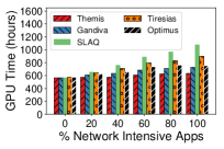
Placement Sensitivity: We analyze the impact on finish-time fairness and cluster efficiency as the fraction of network-intensive apps in our workload increases. We synthetically construct 6 workloads and vary the percentage of network-intensive apps in these workloads across from $0$%-$100$%.

(a) Impact on Max $\rho$

(b) Impact on GPU Time

Figure 13: [Simulator] Impact of placement sensitivity for varying compute-network apps distributions

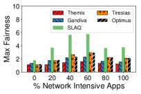
From Figure 13(a), we notice that sharing incentive degrades most when there is a heterogeneous mix of compute and network intensive apps (at 40% and 60%). Themis has a max $\rho$ value closest to $1$ across all these scenarios and is the only scheme to ensure this sharing incentive. When the workload consists solely of network-intensive apps, Themis performs ~$1.24X$, $2.04X$, $1.72X$ and $1.77X$ better than Gandiva, SLAQ, Tiresias, and Optimus respectively on max fairness.

Figure 13(b) captures the impact on cluster efficiency. With only compute-intensive apps, all scheduling schemes utilize the cluster equally efficiently. As the percentage of network intensive apps increases, Themis has lower GPU times to execute the same workload. This means that Themis utilizes the cluster more efficiently than other schemes. In the workload with $100$% network-intensive apps, Themis performs ~8.1% better than Gandiva (state-of-the-art for cluster efficiency).

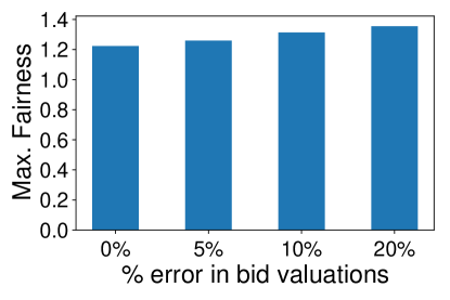
Error Analysis: Here, we evaluate the ability of Themis to handle errors in estimation of number of iterations and the slowdown ($\mathcal{S}$). For this experiment, we assume that all apps are equally susceptible to making errors in estimation. The percentage error is sampled at random from [-$X$, $X$] range for each app. Figure 15 shows the changes in max finish-time fairness as we vary $X$. Even with $X=20$%, the change in max finish-time fairness is just $10.76$% and is not significant.

Figure 14: [Simulator] Impact of error in bid values on max fairness

Figure 15: [Simulator] Strategic lying is detrimental

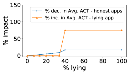
Truth-Telling: To evaluate strategy-proofness, we use simulations. We use a cluster of $64$ GPUs with $8$ identical apps with equivalent placement preferences. The cluster has a single $8$ GPU machine and the others are all $2$ GPU machines. The most preferred allocation in this cluster is the $8$ GPU machine. We assume that there is a single strategically lying app and $7$ truthful apps. In every round of auction it participates in, the lying app over-reports the slowdown with staggered machine placement or under-reports the slowdown with dense machine placement by $X$%. Such a strategy would ensure higher likelihood of winning the $8$ GPU machine. We vary the value of $X$ in the range $[0,100]$ and analyze the lying app’s completion time and the average app completion time of the truthful apps in Figure 15. We see that at first the lying app does not experience any decrease in its own app completion time. On the other hand, we see that the truthful apps do better on their average app completion time. This is because the hidden payment from the partial allocation mechanism in each round of the auction for the lying app remains the same while the payment from the rest of the apps keeps decreasing. We also observe that there is a sudden tipping point at $X>34$%. At this point, there is a sudden increase in the hidden payment for the lying app and it loses a big chunk of resources to other apps. In essence, Themis incentivizes truth-telling.

6.4 Sensitivity Analysis

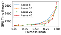
We use simulations to study Themis’s sensitivity to fairness knob $f$ and the lease time. Figure 16 (a) shows the impact on max $\rho$ as we vary the fairness knob $f$. We observe that filtering $(1-f)$ fraction of apps helps with ensuring better sharing incentive. As $f$ increases from $0$ to $0.8$, we observe that fairness improves. Beyond $f=0.8$, max fairness worsens by around a factor of $1.5X$. We see that the quality of sharing incentive, captured by max $\rho$, degrades at $f=1$ because we observe that only a single app with highest $\rho$ value participates in the auction. This app is forced sub-optimal allocations because of poor placement of available resources with respect to the already allocated resources in this app. We also observe that smaller lease times promote better fairness since frequently filtering apps reduces the time that queued apps wait for an allocation.

Figure 16 (b) shows the impact on the efficiency of cluster usage as we vary the fairness knob $f$. We observe that the efficiency decreases as the value of $f$ increases. This is because the number of apps that can bid for an offer reduces as we increase $f$ leading to fewer opportunities for the Arbiter to pack jobs efficiently. Lower lease values mean than models need to be check-pointed more often (GPUs are released on lease expiry) and hence higher lease values are more efficient.

Thus we choose $f=0.8$ and $lease=10$ minutes.

(a) Impact on Max Fairness

(b) Impact on GPU Time

Figure 16: [Simulator] Sensitivity of fairness knob and lease time.

7 Related Work

Cluster scheduling for ML workloads has been targeted by a number of recent works including SLAQ [43], Gandiva [40], Tiresias [13] and Optimus [28]. These systems target different objectives and we compare against them in Section 6.

We build on rich literature on cluster scheduling disciplines [8, 12, 11, 10] and two level schedulers [17, 37, 31]. While those disciplines/schedulers don’t apply to our problem, we build upon some of their ideas, e.g., resource offers in [17]. Sharing incentive was outlined by DRF [8], but we focus on long term fairness with our finish-time metric. Tetris [10] proposes resource-aware packing with an option to trade-off for fairness using multi-dimensional bin-packing as the mechanism for achieving that. In Themis, we instead focus on fairness with an option to trade-off for placement-aware packing, and use auctions as our mechanism.

Some earlier schemes [11, 12] also attempted to emulate the long term effects of fair allocation. Around occasional barriers, unused resources are re-allocated across jobs. Themis differs in many respects: First, earlier systems focus on batch analytics. Second, earlier schemes rely on instantaneous resource-fairness (akin to DRF), which has issues with placement-insensitivity and not accounting for long tasks. Third, in the ML context there are no occasional barriers. While barriers do arise due to synchronization of parameters in ML jobs, they happen at every iteration. Also, resources unilaterally given up by a job may not be usable by another job due to placement sensitivity.

8 Conclusion

In this paper we presented Themis, a fair scheduling framework for ML training workloads. We showed how existing fair allocation schemes are insufficient to handle long-running tasks and placement preferences of ML workloads. To address these challenges we proposed a new long term fairness objective in finish-time fairness. We then presented a two-level semi-optimistic scheduling architecture where ML apps can bid on resources offered in an auction. Our experiments show that Themis can improve fairness and efficiency compared to state of the art schedulers.

Appendix A Appendix

Proof of Theorem 3.1. Examples in Figure 6 and Section 3.1.2 shows that DRF violates SI, EF, and PE. Same examples hold true for LAS policy in Tiresias. The service metric i.e. the GPU in Instance 1 and Instance 2 is the same for A1 and A2 in terms of LAS and is deemed a fair allocation over time. However, Instance 1 violates SI as A1 (VGG16) and A2 (VGG19) would prefer there own independent GPUs and Instance 2 violates EF and PE as A2 (VGG19) prefers the allocation of A1 (Inceptionv3) and PE as the optimal allocation after taking into account placement preferences would interchange the allocation of A1 and A2. ∎

Proof of Theorem 3.2. We first show that the valuation function, $\rho(.)$, for the case of ML jobs is homogeneous. This means that $\rho(.)$ has the following property: $\rho(m*\overrightarrow{G})$ = $m*\rho{\overrightarrow{G}}$.

Consider a job with GPUs spread across a set of some $M$ machines. If we keep this set of machines the same, and increase the number of GPUs allocated on these same set of machines by a certain factor then the shared running time ($T_{sh}$) of this job decreases proportionally by the same factor. This is so because the slowdown, $\mathcal{S}$ remains the same. Slowdown is determined by the slowest network interconnect between the machines. The increased allocation does not change the set of machines $M$. The independent running time ($T_{id}$) remains the same. This means that $\rho$ also proportionally changes by the same factor.

Given, homogeneous valuation functions, the PA mechanism guarantees SP, PE and EF [5]. However, PA violates SI due to the presence of hidden payments. This also make PA not work-conserving. ∎

Proof of Theorem 3.3. With multi-round auctions we ensure truth-telling of $\rho$ estimates in the visibility phase. This is done by the Agentby using the cached $\rho(.)$ estimates from the last auction the app participated in. In case an app gets leftover allocations from the leftover allocation mechanism, the Agentupdates the $\rho$ estimate again by using the cached $\rho(.)$ table. In this way we guarantee SP with multi-round auctions.

As we saw in Theorem 3.2, an auction ensures PE and EF. In each round, we allocate all available resources using auctions. This ensures end-to-end PE and EF.

For maximizing sharing incentive, we always take a fraction $1-f$ of apps in each round. A wise choice of $f$ ensures that we filter in all the apps with $\rho>1$ that have poor sharing incentive. We only auction the resources to such apps which maximizes sharing incentive. ∎

A.1 Workload Details

We experiment with $2$ different traces that have different workload characteristics in both the simulator and the testbed - (i) Workload 1. A publicly available trace of DNN training workloads at Microsoft [20, 25]. We scale-down the trace, using a two week snapshot and focusing on subset of jobs from the trace that correspond to hyper-parameter exploration jobs triggered by Hyperdrive. (ii) Workload 2. We use the app arrival times from Workload 1, generate jobs per app using the successive halving pattern characteristic of the Hyperband algorithm [22]. The distribution of number of tasks per job and number of jobs per app for the two workloads is shown in Figure 17.

(a)

(b)

Figure 17: Details of 2 workloads used for evaluation of Themis

The traces comprise of models from three categories - computer vision (CV - 10%), natural language processing (NLP - 60%) and speech (Speech - 30%). We use the same mix of models for each category as outlined in Gandiva [40]. We summarize the models in Table 4.

	Model	Type	Dataset
10%	Inceptionv3 [34]	CV	ImageNet [7]
	Alexnet [21]	CV	ImageNet
	Resnet50 [16]	CV	ImageNet
	VGG16 [33]	CV	ImageNet
	VGG19 [33]	CV	ImageNet
60%	Bi-Att-Flow [32]	NLP	SQuAD [29]
	LanguageModel [42]	NLP	PTB [23]
	GNMT [39]	NLP	WMT16 [38]
	Transformer [36]	NLP	WMT16
30%	Wavenet [26]	Speech	VCTK [41]
	DeepSpeech [15]	Speech	CommonVoice [6]

Table 4: Models used in our trace.

References

- [1] Apache Hadoop NextGen MapReduce (YARN). Retrieved 9/24/2013, URL: http://hadoop.apache.org/docs/current/hadoop-yarn/hadoop-yarn-site/YARN.html, 2013.
- [2] Apache Hadoop Submarine. https://hadoop.apache.org/submarine/, 2019.
- [3] J. Bergstra, B. Komer, C. Eliasmith, D. Yamins, and D. D. Cox. Hyperopt: a python library for model selection and hyperparameter optimization. Computational Science & Discovery, 8(1), 2015.
- [4] J. Chen, X. Pan, R. Monga, S. Bengio, and R. Jozefowicz. Revisiting distributed synchronous sgd. arXiv preprint arXiv:1604.00981, 2016.
- [5] R. Cole, V. Gkatzelis, and G. Goel. Mechanism design for fair division: allocating divisible items without payments. In Proceedings of the fourteenth ACM conference on Electronic commerce, pages 251–268. ACM, 2013.
- [6] Common Voice Dataset. https://voice.mozilla.org/.
- [7] J. Deng, W. Dong, R. Socher, L.-J. Li, K. Li, and L. Fei-Fei. Imagenet: A large-scale hierarchical image database. In 2009 IEEE conference on computer vision and pattern recognition, pages 248–255. Ieee, 2009.
- [8] A. Ghodsi, M. Zaharia, B. Hindman, A. Konwinski, S. Shenker, and I. Stoica. Dominant resource fairness: Fair allocation of multiple resource types. In NSDI, 2011.
- [9] D. Golovin, B. Solnik, S. Moitra, G. Kochanski, J. Karro, and D. Sculley. Google vizier: A service for black-box optimization. In KDD, 2017.
- [10] R. Grandl, G. Ananthanarayanan, S. Kandula, S. Rao, and A. Akella. Multi-resource packing for cluster schedulers. ACM SIGCOMM Computer Communication Review, 44(4):455–466, 2015.
- [11] R. Grandl, M. Chowdhury, A. Akella, and G. Ananthanarayanan. Altruistic scheduling in multi-resource clusters. In 12th USENIX Symposium on Operating Systems Design and Implementation (OSDI 16), pages 65–80, 2016.
- [12] R. Grandl, S. Kandula, S. Rao, A. Akella, and J. Kulkarni. GRAPHENE: Packing and Dependency-Aware Scheduling for Data-Parallel Clusters. In 12th USENIX Symposium on Operating Systems Design and Implementation (OSDI 16), pages 81–97, 2016.
- [13] J. Gu, M. Chowdhury, K. G. Shin, Y. Zhu, M. Jeon, J. Qian, H. Liu, and C. Guo. Tiresias: A GPU cluster manager for distributed deep learning. In 16th USENIX Symposium on Networked Systems Design and Implementation (NSDI 19), pages 485–500, 2019.
- [14] Gurobi Optimization. http://www.gurobi.com/.
- [15] A. Hannun, C. Case, J. Casper, B. Catanzaro, G. Diamos, E. Elsen, R. Prenger, S. Satheesh, S. Sengupta, A. Coates, et al. Deep speech: Scaling up end-to-end speech recognition. arXiv preprint arXiv:1412.5567, 2014.
- [16] K. He, X. Zhang, S. Ren, and J. Sun. Deep residual learning for image recognition. In Proceedings of the IEEE conference on computer vision and pattern recognition, pages 770–778, 2016.
- [17] B. Hindman, A. Konwinski, M. Zaharia, A. Ghodsi, A. D. Joseph, R. H. Katz, S. Shenker, and I. Stoica. Mesos: A platform for fine-grained resource sharing in the data center. In NSDI, 2011.
- [18] M. Isard, V. Prabhakaran, J. Currey, U. Wieder, K. Talwar, and A. Goldberg. Quincy: fair scheduling for distributed computing clusters. In Proceedings of the ACM SIGOPS 22nd symposium on Operating systems principles, pages 261–276. ACM, 2009.
- [19] M. Jeon, S. Venkataraman, A. Phanishayee, J. Qian, W. Xiao, and F. Yang. Analysis of Large-Scale Multi-Tenant GPU Clusters for DNN Training Workloads. In USENIX ATC, 2019.
- [20] M. Jeon, S. Venkataraman, A. Phanishayee, J. Qian, W. Xiao, and F. Yang. Analysis of Large-Scale Multi-Tenant GPU Clusters for DNN Training Workloads. In USENIX ATC, 2019.
- [21] A. Krizhevsky, I. Sutskever, and G. E. Hinton. Imagenet classification with deep convolutional neural networks. In Advances in neural information processing systems, pages 1097–1105, 2012.
- [22] L. Li, K. Jamieson, G. DeSalvo, A. Rostamizadeh, and A. Talwalkar. Hyperband: A novel bandit-based approach to hyperparameter optimization. arXiv preprint arXiv:1603.06560, 2016.
- [23] M. Marcus, B. Santorini, and M. A. Marcinkiewicz. Building a large annotated corpus of english: The penn treebank. 1993.
- [24] Microsoft Azure. https://azure.microsoft.com/en-us/.
- [25] Microsoft Philly Trace. https://github.com/msr-fiddle/philly-traces, 2019.
- [26] A. v. d. Oord, S. Dieleman, H. Zen, K. Simonyan, O. Vinyals, A. Graves, N. Kalchbrenner, A. Senior, and K. Kavukcuoglu. Wavenet: A generative model for raw audio. arXiv preprint arXiv:1609.03499, 2016.
- [27] K. Ousterhout, P. Wendell, M. Zaharia, and I. Stoica. Sparrow: distributed, low latency scheduling. In SOSP, pages 69–84, 2013.
- [28] Y. Peng, Y. Bao, Y. Chen, C. Wu, and C. Guo. Optimus: an efficient dynamic resource scheduler for deep learning clusters. In Proceedings of the Thirteenth EuroSys Conference, page 3. ACM, 2018.
- [29] P. Rajpurkar, J. Zhang, K. Lopyrev, and P. Liang. Squad: 100,000+ questions for machine comprehension of text. arXiv preprint arXiv:1606.05250, 2016.
- [30] J. Rasley, Y. He, F. Yan, O. Ruwase, and R. Fonseca. Hyperdrive: Exploring hyperparameters with pop scheduling. In Proceedings of the 18th ACM/IFIP/USENIX Middleware Conference, pages 1–13. ACM, 2017.
- [31] M. Schwarzkopf, A. Konwinski, M. Abd-El-Malek, and J. Wilkes. Omega: flexible, scalable schedulers for large compute clusters. In Eurosys, 2013.
- [32] M. Seo, A. Kembhavi, A. Farhadi, and H. Hajishirzi. Bidirectional attention flow for machine comprehension. arXiv preprint arXiv:1611.01603, 2016.
- [33] K. Simonyan and A. Zisserman. Very deep convolutional networks for large-scale image recognition. arXiv preprint arXiv:1409.1556, 2014.
- [34] C. Szegedy, V. Vanhoucke, S. Ioffe, J. Shlens, and Z. Wojna. Rethinking the inception architecture for computer vision. In Proceedings of the IEEE conference on computer vision and pattern recognition, pages 2818–2826, 2016.
- [35] H. R. Varian. Equity, envy, and efficiency. Journal of Economic Theory, 9(1):63 – 91, 1974.
- [36] A. Vaswani, N. Shazeer, N. Parmar, J. Uszkoreit, L. Jones, A. N. Gomez, Ł. Kaiser, and I. Polosukhin. Attention is all you need. In Advances in neural information processing systems, pages 5998–6008, 2017.
- [37] A. Verma, L. Pedrosa, M. Korupolu, D. Oppenheimer, E. Tune, and J. Wilkes. Large-scale cluster management at google with borg. In Eurosys, 2015.
- [38] WMT16 Dataset. http://www.statmt.org/wmt16/.
- [39] Y. Wu, M. Schuster, Z. Chen, Q. V. Le, M. Norouzi, W. Macherey, M. Krikun, Y. Cao, Q. Gao, K. Macherey, et al. Google’s neural machine translation system: Bridging the gap between human and machine translation. arXiv preprint arXiv:1609.08144, 2016.
- [40] W. Xiao, R. Bhardwaj, R. Ramjee, M. Sivathanu, N. Kwatra, Z. Han, P. Patel, X. Peng, H. Zhao, Q. Zhang, et al. Gandiva: Introspective cluster scheduling for deep learning. In 13th USENIX Symposium on Operating Systems Design and Implementation (OSDI 18), pages 595–610, 2018.
- [41] J. Yamagishi. English multi-speaker corpus for cstr voice cloning toolkit. URL http://homepages. inf. ed. ac. uk/jyamagis/page3/page58/page58. html, 2012.
- [42] W. Zaremba, I. Sutskever, and O. Vinyals. Recurrent neural network regularization. arXiv preprint arXiv:1409.2329, 2014.
- [43] H. Zhang, L. Stafman, A. Or, and M. J. Freedman. Slaq: quality-driven scheduling for distributed machine learning. In Proceedings of the 2017 Symposium on Cloud Computing, pages 390–404. ACM, 2017.