Analytic and directional wavelet packets in the space of periodic signals
Abstract
The paper presents a versatile library of analytic and quasi-analytic complex-valued wavelet packets (WPs) which originate from discrete splines of arbitrary orders. The real parts of the quasi-analytic WPs are the regular spline-based orthonormal WPs designed in [2]. The imaginary parts are the so-called complementary orthonormal WPs, which, unlike the symmetric regular WPs, they are antisymmetric. Tensor products of 1D quasi-analytic WPs provide a diversity of 2D WPs oriented in multiple directions. For example, a set of the fourth-level WPs comprises 62 different directions. The designed computational scheme in the paper enables us to get fast and easy implementation of the WP transforms. The presented WPs proved to be efficient in signal/image processing applications such as restoration of images degraded by either additive noise or missing of up to 90% of their pixels.
1 Introduction
Since the introduction in Kingsbury [17, 18] of complex wavelet transforms implemented by the dual-tree scheme, the complex wavelets (DT_CW), wavelet frames and wavelet packets (WPs) have become a field of active research that appears in multiple applications ([13, 15, 14, 26, 24, 5, 10, 11], to name a few). The advantages of the DT_CWs over the standard real wavelet transforms stem from their approximate shift invariance and some directionality inherent to tensor-products of the DT_CWs.
However, the directionality of the DT_CWs is very limited (only 6 directions) and this is a drawback for image processing applications. The tight tensor-product complex wavelet frames TP_CTFn with different number of directions, are designed in [10, 11] and some of them, in particular TP_CTF6 and TP_CTF, demonstrate excellent performance (in terms of PSNR) for image denoising and inpainting. The number of directions in both 2D TP_CTF6 and TP_CTF frames is 14 and remains the same for all decomposition levels.
Some of the disadvantages of the above 2D TP_CTF6 and TP_CTF frames are mentioned in [6]. For example, “limited and fixed number of directions is undesirable in practice especially when the resolution of an image is very high that requires large number of directional filters in order to capture as many features with different orientations as possible” ([6]). In addition, “due to the fixed number of 1D filters, the number of free parameters is limited which prevents the search of optimal filter bank systems for image processing” ([6]).
According to [6], the remedy for the above shortcomings is in the incorporation of the two-layer structure that is inherent in the TP_CTF6 and TP_CTF frames into directional filter banks introduced in [12, 27].
The complex wavelet packets (Co_WPs) is an alternative way to overcome the above disadvantages. The first version of complex WPs appears in [13] after the introduction of the complex wavelets by Kingsbury. The complex wavelet transforms in [13, 15, 14] are extended to the Co_WP transforms by the application of the same filters as used in the DT_CW transforms to the high-frequency bands. Although the low- and high-frequency bands in DT_CW are approximately analytic, this is not the case for the Co_WPs designed in [13, 15, 14]. In addition, as shown in [5] (Fig. 1), much energy passes into the negative half-bands of the spectra. Another approach to the design of Co_WPs is described in [5]. It is suggested in [5] that in order to retain an approximate analyticity of the dual-tree WP transforms, the filter banks for the second decomposition of the transforms should be the same for both stems of the tree.
Although the potential advantages of the Co_WP transforms are apparent, so far, to the best of our knowledge, none of the Co_WP schemes in the literature have the desired properties such as perfect frequency separation, Hilbert transform relation between real and imaginary parts of the Co_WPs, orthonormality of shifts of real and imaginary parts of the Co_WPs, unlimited number of directions in the multidimensional case, a variety of free parameters, and fast and easy implementation.
Our motivation in this paper is to fill this gap. We design a family of Co_WP transforms which possess all the above properties. As a base for the design, we use the family of discrete-time WPs originated from periodic discrete splines of different orders that are described in [2] (Chapter 4). The wavelet packets , where is the decomposition level, is the index of the related frequency band and is the order of the generating discrete spline, are symmetric, well localized in time domain (although are not compactly supported), their DFTs spectra are flat, and provide a refined split of the frequency domain. The WP transforms are executed in the frequency domain using the Fast Fourier transform (FFT). By varying the order , we can supply the WPs with any number of local vanishing moments without increase of the computational cost. Different combinations of the shifts in these WPs provide a variety of orthonormal bases of the space of -periodic signals.
To derive the Co_WPs, we expand the WPs to periodic analytic discrete-time signals , where is the discrete periodic Hilbert transform (HT) of the WP . The waveforms are antisymmetric, and for all orthonormal properties similar to the properties of the WPs take place. To achieve orthonormality, the waveforms are slightly corrected at the expense of minor deviation from antisymmetry and we get a new orthonormal complimentary WP (cWP) system , where for , the WPs satisfy . The magnitude spectra of the cWPs coincide with the spectra of the respective WPs and, similarly to the WPs , the cWPs provide a variety of orthonormal bases for the space of -periodic signals.
Correspondingly, we define the quasi-analytic WP systems (qWP) as
where all the WPs with indices other than are analytic. For the implementation of the transforms with the complex qWPs we do not use the dual-tree scheme with different filter banks for real and imaginary wavelets but use the scheme with a single complex filter bank in the first step of the transform, and a real filter bank in the additional steps.
A dual-tree structure type appears in the 2D case when two sets of qWPs are defined as the tensor products of 1D qWPs
| (1.1) |
and processing with the qWPs is executed separately.
The real and imaginary parts of the qWPs are the 2D waveforms oriented in multiple directions, specifically the directions at the -th decomposition level. Such an abundant directionality proved to be efficient in the examples on image denoising and inpainting. It is worth mentioning that the WPs of one- and two-dimensions have a localized oscillating structure, which is useful for detection of transient oscillating events in 1D signals and oscillating patterns in the images (for example, “Barbara” in Fig. 7.2).
Both one- and two-dimensional transforms are implemented in a very fast ways by using FFT.
The paper is organized as follows: Section 2 outlines briefly periodic discrete-time WPs originated from discrete splines and corresponding transforms that form a basis for the design of Co_WPs. The analysis and synthesis filter banks for the WP transforms are described. Section 3 outlines the construction of discrete-time periodic analytic signals. This section also introduces complimentary sets of WPs (cWPs), analytic and quasi-analytic WPs (qWPs). Section 4 describes the implementation of the cWP and qWP transforms. The filter banks for one step of analysis and synthesis transforms are introduced. It is interesting to note that subsequent application of the direct and inverse qWP filter banks to a signal produces the analytic signal . All the subsequent steps of cWP and qWP transforms are implemented with the same filter banks and as used in the above WP transforms (section 2). Section 5 extends the design of 1D qWPs to the 2D case. The 2D qWPs are defined via tensor products as shown in Eq. (1.1). Directionality of the 2D qWPs is discussed. Section 6 describes the implementation of the 2D qWP transforms by a dual-tree. Section 7 presents a few experimental results for images restoration degraded by either strong additive noise or by missing many of the pixels. In one example, both the degradation sources are present. Section 8 discusses the results. The Appendix contains proof of a proposition.
Notations and abbreviations
, , and is a space of real-valued -periodic signals. is the space of two-dimensional -periodic arrays in both vertical and horizontal directions. .
A signal is represented by its inverse discrete Fourier transform (DFT)
| (1.2) |
where means complex conjugate. In particular, and are real numbers.
The DFT of an -periodic signal is . The abbreviation PR means perfect reconstruction. The abbreviations 1D and 2D mean one-dimensional and two-dimensional, respectively. FFT is the fast Fourier transform, HT is the Hilbert transform, is the discrete periodic HT of a signal .
The abbreviations WP, cWP and qWP mean wavelet packets (typically spline-based wavelet packets ), complimentary wavelet packets and quasi-analytic wavelet packets , respectively, in 1D case, and wavelet packets , complimentary wavelet packets and quasi-analytic wavelet packets , respectively, in 2D case.
| (1.3) |
Peak Signal-to-Noise ratio (PSNR) in decibels (dB) is
SBI stands for split Bregman iterations and p-filter means periodic filter.
2 Outline of orthonormal WPs originated from discrete splines: preliminaries
This section provides a brief outline of periodic discrete-time wavelet packets originated from discrete splines and corresponding transforms. For details see Chapter 4 in [2].
2.1 Periodic discrete splines
The centered span-two -periodic discrete B-spline of order is defined as the IDFT of the sequence
The B-splines are non-negative symmetric finite-length signals (up to periodization). Only the samples are non-zero.
The signals which are referred to as discrete splines, form an -dimensional subspace of the space whose basis consists of two-sample shifts of the B-spline . Here is a real-valued sequence. The DFT of the discrete spline is
A discrete spline is defined through its inverse DFT (iDFT):
where is defined in Eq. (1.3).
Proposition 2.1 ([2], Proposition 3.6)
Two-sample shifts of the discrete splines form an orthonormal basis of the subspace .
The orthogonal projection of a signal onto the space is the signal such that
| (2.1) |
2.2 Orthogonal complement for subspace
The orthogonal complement for in the signal space is denoted by . Thus, . The orthonormal basis in the subspace is formed by the two-sample shifts of the discrete spline , which is defined through its inverse DFT (iDFT):
Proposition 2.2 ([2], Proposition 4.1)
The orthogonal projection of a signal onto the space is the signal such that
| (2.2) |
The signals and are referred to as the discrete-spline wavelet packets of order from the first decomposition level . They are the impulse responses of the low- and high-pass periodic filters (p-filters) and , respectively.
Remark 2.1
We emphasise that the DFTs and .
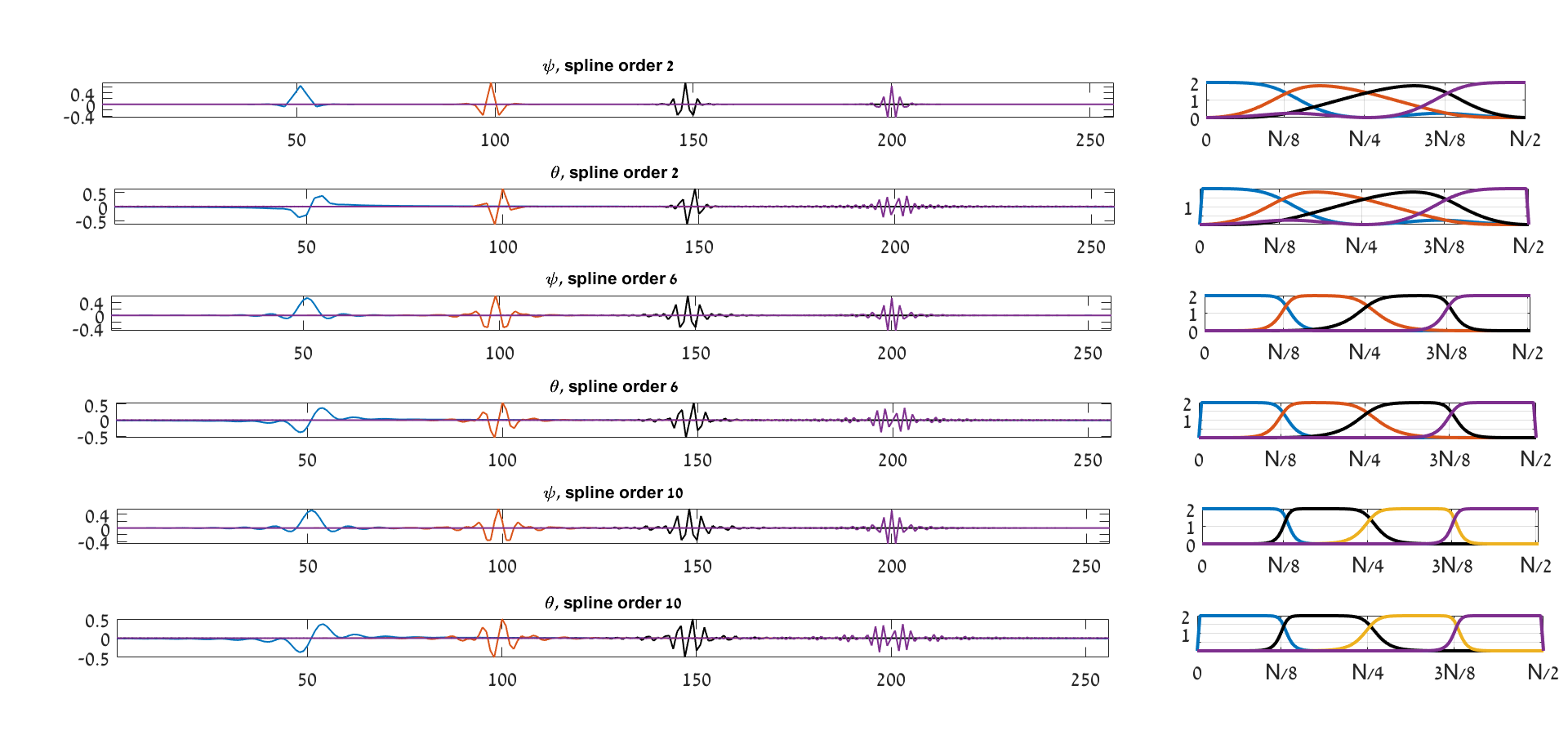
Figure 2.1 displays the discrete-spline wavelet packets and of different orders and magnitudes of their DFT spectra (which are the p-filters and magnitude responses). It is seen that the wavelets are well localized in time domain. The spectra are flat and their shapes tend to rectangular as their orders increase.
2.3 One-level wavelet packet transform of a signal
The transform of a signal into the pair of signals from is referred to as the one-level wavelet packet transform (WPT) of the signal . According to Propositions 2.1 and 2.2, the transform is implemented by filtering with time-reversed half-band low- and high-pass p-filters and , respectively, which is followed by downsampling. Thus the p-filters and form a critically sampled analysis p-filter bank . Eqs. (2.1) and (2.2) imply that its modulation matrix is
| (2.3) |
The analysis modulation matrix , as well as the matrix are unitary matrices. Therefore, the synthesis modulation matrix is
| (2.6) |
Consequently, the synthesis p-filter bank coincides with the analysis p-filter bank and, together, they form a perfect reconstruction (PR) p-filter bank.
The one-level WP transform of a signal and its inverse are represented in a matrix form:
| (2.7) |
where .
2.4 Extension of transforms to deeper decomposition levels
2.4.1 Second-level p-filter banks
The signals belong to the space . The space can be split into mutually orthogonal subspaces, which we denote by and , in a way that is similar to the split of the space . Projection of a signal onto these subspaces and the inverse operation are done using the analysis and synthesis p-filter banks (Eq. 2.8), which operate in the space . The frequency responses of the p-filters are
| (2.8) |
where and are defined in Eq. (2.3). The impulse responses of the p-filters and are orthogonal to each other in the space and their 2-sample shifts are mutually orthogonal
The orthogonal projections of a signal onto the subspaces and are
where The modulation matrices of the p-filter bank are
| (2.9) |
where the modulation matrices and are defined in Eqs. (LABEL:1a_modma10) and (2.6), respectively.
2.4.2 Second-level WPTs
By the application of the analysis p-filter bank (section 2.4.1 and Eq. 2.8) to the signals that belong to , we get their orthogonal projections and onto the subspaces and :
where
The signal is a linear combination of 2-sample shifts of the discrete-spline WP , therefore . Its DFT is
| (2.10) |
Proposition 2.3 ([2])
The norms of the signals are equal to one. The 4-sample shifts of this signal are mutually orthogonal and signals with different indices are orthogonal to each other.
Thus, the signal space splits into four mutually orthogonal subspaces whose orthonormal bases are formed by 4-sample shifts of the signals , which are referred to as the second-level discrete-spline wavelet packets of order .
The orthogonal projection of a signal onto the subspace is the signal
Practically, derivation of the wavelet packet transform coefficients from and the inverse operation are implemented using Eq. (2.7), while the transform are implemented similarly using the modulation matrices of the p-filter bank defined in Eq. (2.9). The second-level wavelet packets are derived from the first-level wavelet packets by filtering the latter with the p-filters .
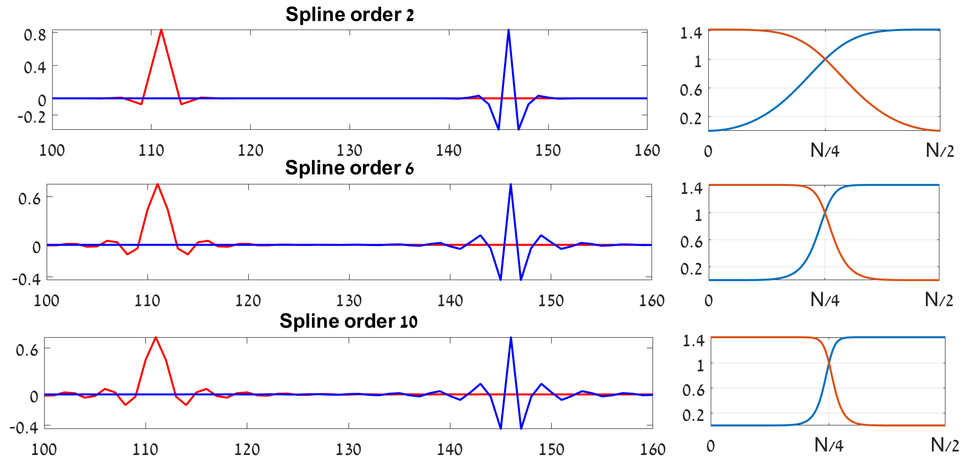
Figure 2.2 displays the second-level wavelet packets originating from discrete splines of orders 2, 6 and 10 and their DFTs. One can observe that the wavelet packets are symmetric and well localized in time domain. Their spectra are flat and their shapes tend to rectangular as their orders increase. They split the frequency domain into four quarter-bands.
2.4.3 Transforms to deeper levels
The WPTs to deeper decomposition levels are implemented iteratively, while the transform coefficients are derived by filtering the coefficients with the p-filters where and The transform coefficients are , where the signals are normalized, orthogonal to each other in the space , and their sample shifts are mutually orthogonal. They are referred to as level- discrete-spline wavelet packets of order . The set constitutes an orthonormal basis of the space and generates its split into orthogonal subspaces. The next-level wavelet packets are derived by filtering the wavelet packets with the p-filters such that
| (2.11) |
Note that the frequency response of an level p-filter is
A scheme of fast implementation of the discrete-spline-based WPT is described in [2]. The transforms are executed in the spectral domain using the Fast Fourier transform (FFT) by the application of critically sampled two-channel filter banks to the half-band spectral components of a signal. For example, the Matlab execution of the 8-level 12-th-order WPT of a signal comprising 245760 samples, takes 0.2324 seconds.
2.5 2D WPTs
A standard way to extend the one-dimensional (1D) WPTs to multiple dimensions is the tensor-product extension. The 2D one-level WPT of a signal which belongs to , consists of the application of 1D WPT to columns of , which is followed by the application of the transform to rows of the coefficients array. As a result of the 2D WPT of signals from , the space becomes split into four mutually orthogonal subspaces
The subspace is a linear hull of two-sample shifts of the 2D wavelet packets
that form an orthonormal basis of . The orthogonal projection of the signal onto the subspace is the signal such that
The 2D wavelet packets are They are normalized and orthogonal to each other in the space . It means that
. Their two-sample shifts in either direction are mutually orthogonal. The transform coefficients are
By the application of the above transforms iteratively to blocks of the transform coefficients down to -th level, we get that the space is decomposed into mutually orthogonal subspaces The orthogonal projection of the signal onto the subspace is the signal such that
The 2D tensor-product wavelet packets are well localized in the spatial domain, their 2D DFT spectra are flat and provide a refined split of the frequency domain of signals from 111Especially it is true for WPs derived from higher-order discrete splines. The drawback is that the wavelet packets are oriented in ether horizontal or vertical directions or are not oriented at all.
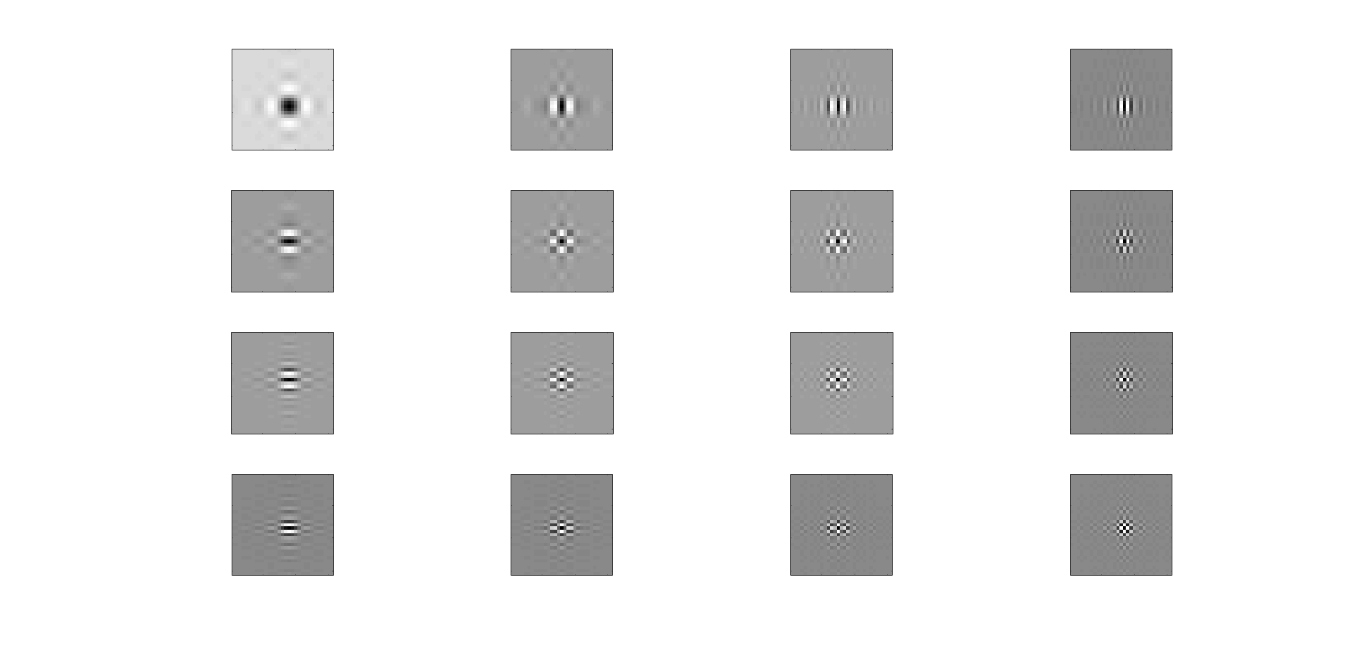
Figure 2.3 displays the tenth-order 2D wavelet packets from the second decomposition level and their magnitude spectra.
3 (Quasi-)analytic and complementary WPs
In this section we define analytic and the so-called quasi-analytic WPs related to the discrete-spline-based WPs discussed in Section 2 and introduce an orthonormal set of waveforms which are complementary to the above WPs.
3.1 Analytic periodic signals
A signal is represented by its inverse DFT. Then, Eq. (1.2) can be written as follows:
Define the real-valued signal and two complex-valued signals and such that
| (3.1) |
The signals’ DFT spectra are
| (3.2) |
The spectrum of comprises only non-negative frequencies and vice versa for . and . The signals are referred to as periodic analytic signals.
The signal’s DFT spectrum is
Thus, the signal where can be regarded as the Hilbert transform (HT) of a discrete-time periodic signal , (see [20], for example).
Proposition 3.1
-
1.
The HT is invariant with respect to circular shift in . That means that is the HT of .
-
2.
If the signal is symmetric about a grid point than is antisymmetric about K and .
-
3.
Assume that a signal and . Then,
-
(a)
The norm of its HT is .
-
(b)
Magnitude spectra of the signals and coincide.
-
(a)
Proof:
-
1.
The DFT of the signal is . Denote by the analytic signal related to . Equation (3.2) implies that . Consequently, . The same relation holds for .
-
2.
Assume that is symmetric about . Then, its DFT is
Then, due to Eq. (3.1), and . Extension of the proof to is straightforward.
-
3.
-
(a)
The squared norm is
-
(b)
The coincidence of the magnitude spectra is straightforwared.
-
(a)
3.2 Analytic WPs
The analytic spline-based WPs and their DFT spectra are derived from the corresponding WPs in line with the scheme in Section 3.1. Recall that for all , the DFT and for all , the DFT .
Denote by the discrete periodic HT of the wavelet packet , such that the DFT is
Then, the corresponding analytic WPs are
Properties of the analytic WPs
-
1.
The DFT spectra of the analytic WPs and are located within the bands and , respectively.
-
2.
The real component is the same for both WPs . It is a symmetric oscillating waveform.
-
3.
The HT WPs are antisymmetric oscillating waveforms.
-
4.
For all , the norms . Their magnitude spectra coincide with the magnitude spectra of the respective WPs .
-
5.
When or , the magnitude spectra of coincide with that of everywhere except for the points or respectively, and the waveforms’ norms are no longer equal to 1.
Properties in items 3–5 follow directly from Proposition 3.1.
Proposition 3.2
For all , the shifts of the HT WPs are orthogonal to each other in the space . The orthogonality does not take place for for and .
Proof: The inner product is
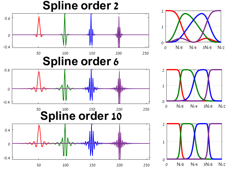
Figure 3.1 displays the wavelet packets and and their magnitude spectra.
3.3 Complementary set of wavelet packets and quasi-analytic WPs
3.3.1 Complementary orthonormal WPs
The discrete-spline-based WPs are normalized and their -sample shifts are mutually orthogonal. Combinations of shifts of several wavelet packets can form orthonormal bases for the signal space . On the other hand, it is not true for the set of the antysymmetric waveforms, which are the HTs of the WPs . At the decomposition level m, the waveforms are normalized and their -sample shifts are mutually orthogonal, but the norms of the waveforms and are close but not equal to 1 and their shifts are not mutually orthogonal. It happens because the values and are missing in their DFT spectra222Recall that these values are real. This keeping in mind, we upgrade the set in the following way.
Define a set of signals from the space via their DFTs:
| (3.3) |
For all the signals coincide with .
Proposition 3.3
- -
-
The magnitude spectra coincide with the magnitude spectra of the respective WPs .
- -
-
For any and the signals are antisymmetric oscillating waveforms. For and , the shapes of the signals are near antisymmetric.
- -
-
The orthonormality properties that are similar to the properties of WPs hold for the signals such that
Figure 3.2 displays the signals and , from the second decomposition level and their magnitude spectra. Lack of the values and in the DFTs of , are seen. Addition of and to the above spectra results in the antisymmetry distortion.
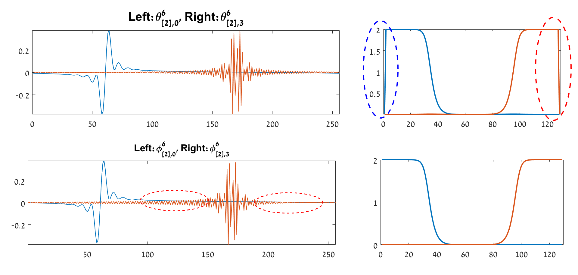
We call the signals , the complementary wavelet packets (cWPs). Similarly to the WPs differenent combinations of the cWPs can provide differenent orthonormal bases for the space . These can be, for example, the wavelet bases
or a Best Basis [7] type.
3.3.2 Quasi-analytic WPs
The sets of complex-valued WPs, which we refer to as the quasi-analytic wavelet packets (qWP), are defined as
where are the cWPs defined in Eq. (3.3). The qWPs differ from the analytic WPs by the addition of the two values and into their DFT spectra, respectively. For a given decomposition level , these values are zero for all except for and . It means that for all except for and , the qWPs are analytic. The DFTs of qWPs are
| (3.7) | |||||
| (3.11) |
3.3.3 Design of cWPs and qWPs
The DFTs of the first-level WPs are
where the sequence is defined in Eq. (1.3). Consequently, the DFTs of the first-level cWPs are
| (3.20) |
Due to Eq. (2.10), the DFT of the second-level WPs are
| (3.23) | |||||
| (3.24) |
For example, assume then we have
Keeping in mind that the sequence is periodic, we have that the DFT of the corresponding cWP is
Similar relations hold for all the second-level cWPs and a general statement is true.
Proposition 3.4
Assume that for a WP the relation in Eq. (2.11) holds. Then, for the cWP we have
Corollary 3.5
Assume that for a WP , the relation in Eq. (2.11) holds. Then, for the qWP we have
| (3.25) |
4 Implementation of cWP and qWP transforms
Implementation of transforms with WPs was discussed in Section 2. In this section, we extent that the transform scheme to the transforms with cWPs and qWPs .
4.1 One-level transforms
Denote by the subspace of the signal space , which is the linear hull of the set . The signals from the set form an orthonormal basis of the subspace . Denote by the orthogonal complement of the subspace in the space . The signals from the set form an orthonormal basis of the subspace .
Proposition 4.1
The orthogonal projections of a signal onto the spaces are the signals such that
The DFTs of the first-level cWPs are given in Eq. (3.20).
The transforms and back are implemented using the analysis and the synthesis modulation matrices:
| (4.1) |
The sequences and are given in Eq. (2.3).
Define the p-filters
Equation (3.7) implies that their frequency responses are
Thus, the analysis modulation matrices for the p-filters are
| (4.6) | |||||
| (4.9) |
where the modulation matrix is defined in Eq. (2.3) and is defined in Eq. (4.1). Application of the matrices to the vector produces the vectors
Define the matrices and apply these matrices to the vectors
. Here the modulation matrix is defined in Eq. (2.6) and is defined in Eq. (4.1).
Proposition 4.2
The following relations hold
where is the HT of the signal and are the analytic signals associated with .
Proof: In Appendix section LABEL:sec:ap2
Definition 4.3
The matrices and are called the analysis and synthesis modulation matrices for the qWP transform, respectively.
Corollary 4.4
Successive application of filter banks defined by the analysis and synthesis modulation matrices and to a signal produces the analytic signals associated with .
Corollary 4.5
A signal is represented by the redundant orthonormal system
Thus, the system
form a tight frame of the space .
4.2 Multi-level transforms
It was explained in Section 2.4.2 that the second-level transform coefficients are
The frequency responses of the p-filters are given in Eq. (2.8) and Eq. (3.24). Recall that . The direct and inverse transforms are implemented using the analysis and synthesis modulation matrices and , that are defined in Eqs. (2.3) and (2.6) respectively:
where
The second-level transform coefficients are
We emphasize that the p-filters for the transform are the same that the p-filters for the transform . Therefore, the direct and inverse transforms are implemented using the same analysis and synthesis modulation matrices and . Apparently, it is the case also for the transforms . The transforms to subsequent decomposition levels are implemented in an iterative way:
where
and vice versa for , and .
By the application of the inverse DFT to the arrays , we get the arrays
of the transform coefficients with the qWPs .
Remark 4.1
We stress that by operating on the transform coefficients , we simultaneously operate on the arrays and , which are the coefficients for the transforms with the WPs and cWPs , respectively. The execution speed of the transform with the qWPs is the same as the speed of the transforms with either WPs or cWPs .
The transforms are executed in the spectral domain using the FFT by the application of critically sampled two-channel filter banks to the half-band spectral components of a signal.
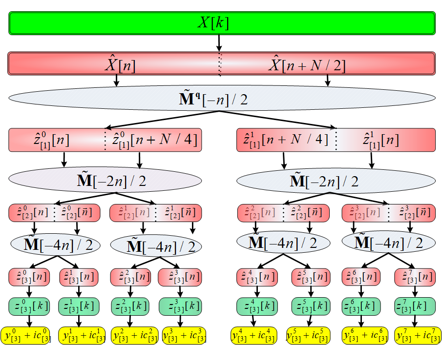
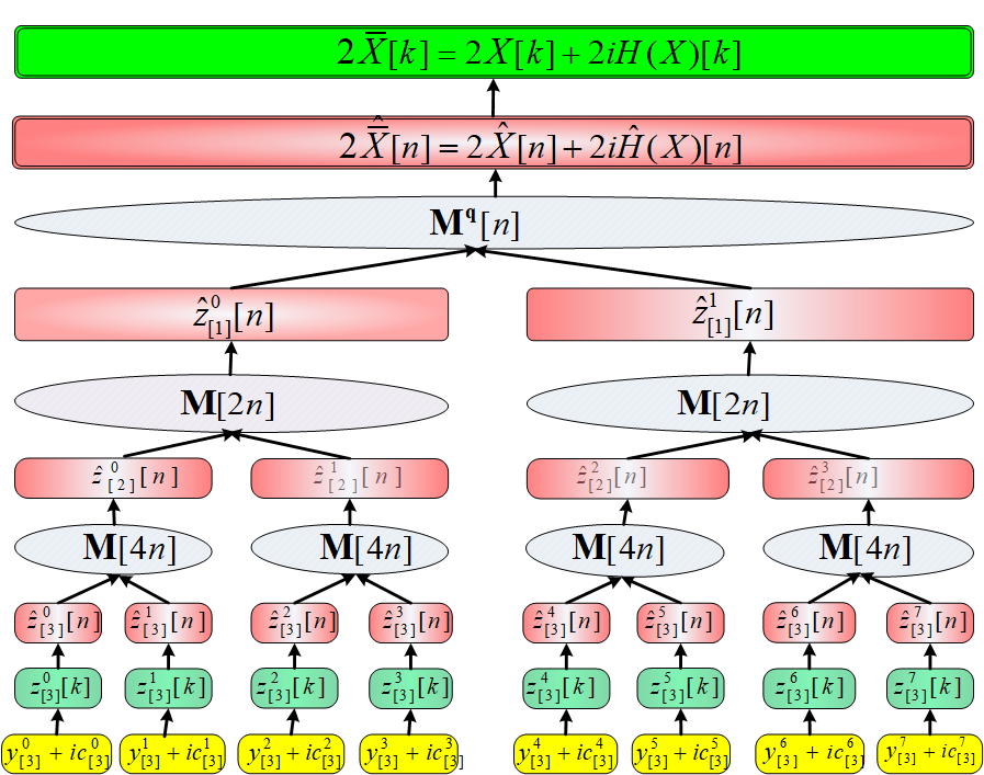
The diagrams in Figs. 4.1 and 4.2 illustrate the three-level forward and inverse qWPTs of a signal with quasi-analytic wavelet packets, which use the analysis and the synthesis modulation matrices, respectively, for the transforms to and from the first decomposition level, respectively, and the modulation matrices and for the subsequent levels.
Remark 4.2
The decomposition of a signal down to the -th level produces transform coefficients . Such a redundancy provides many options for the signal reconstruction. Some of them are listed below.
- •
-
•
Combination of bases compiled from both and WPs generates a tight frame of the space with redundancy rate 2. The bases for and can have a different structure.
-
•
Frames with increased redundancy rate. For example, a combined reconstruction from several decomposition levels.
The collection of WPs and cWPs , which originate from discrete splines of different orders , provides a variety of waveforms that are (anti)symmetric, well localized in time domain. Their DFT spectra are flat and the spectra shapes tend to rectangles when the order increases. Therefore, they can be utilized as a collection of band-pass filters which produce a refined split of the frequency domain into bands of different widths. The (c)WPs can be used as testing waveforms for the signal analysis, such as a dictionary for the Matching Pursuit procedures [19, 3].
5 Two-dimensional complex wavelet packets
A standard design scheme for 2D wavelet packets is outlined in Section 2.5. The 2D wavelet packets are defined as the tensor products of 1D WPs such that
The -sample shifts of the WPs in both directions form an orthonormal basis for the space of arrays that are -periodic in both directions. The DFT spectrum of such a WP is concentrated in four symmetric spots in the frequency domain as it is seen in Fig. 2.3.
Similar properties are inherent to the 2D cWPs such that
5.1 Design of 2D directional WPs
5.1.1 2D complex WPs and their spectra
The WPs as well as the cWPs lack the directionality property which is needed in many applications that process 2D data. However, real-valued 2D wavelet packets oriented in multiple directions can be derived from tensor products of complex quasi-analytic qWPs .
The complex 2D qWPs are defined as follows:
where and . The real and imaginary parts of these 2D qWPs are
| (5.1) |
| (5.2) |
The DFT spectra of the 2D qWPs are the tensor products of the one-sided spectra of the qWPs:
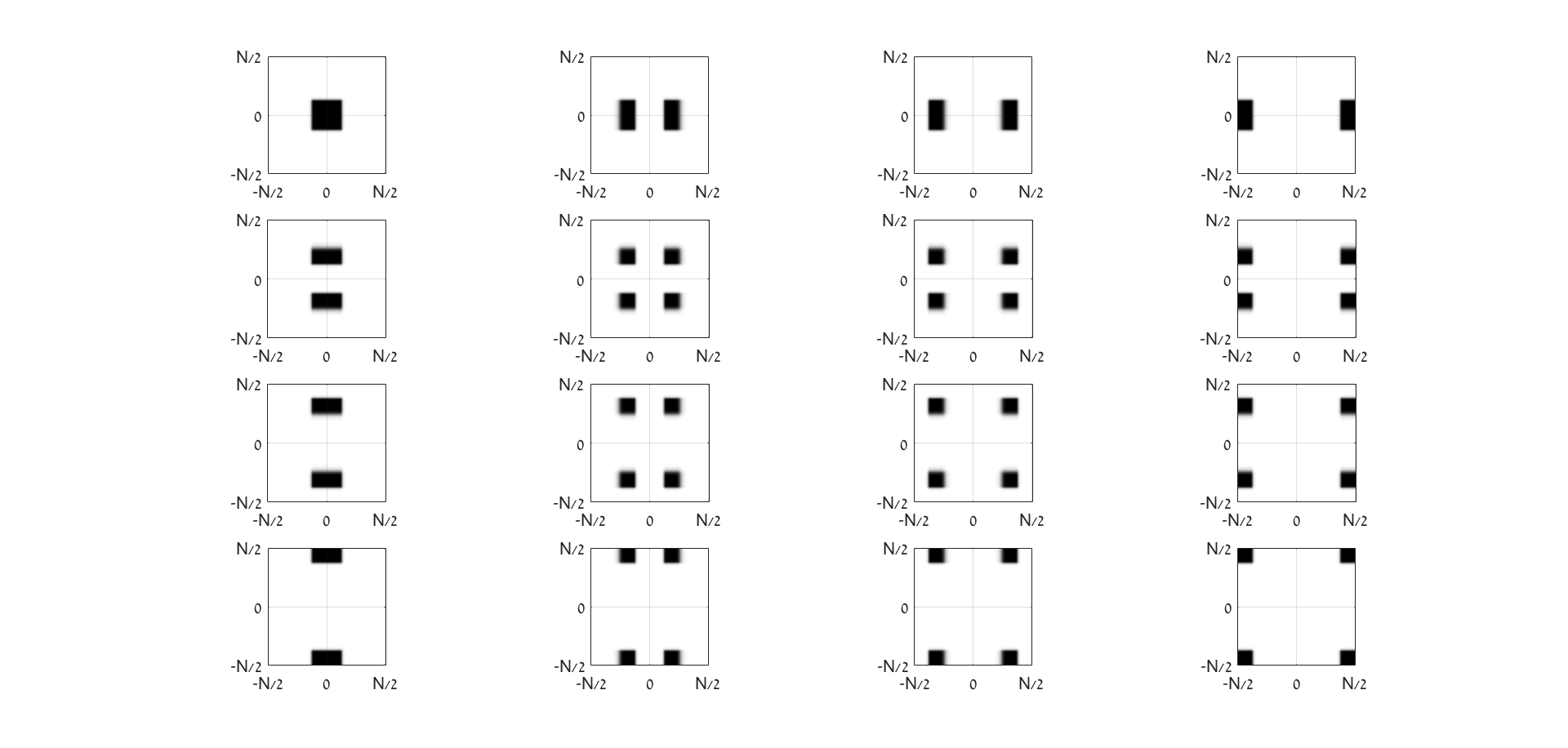
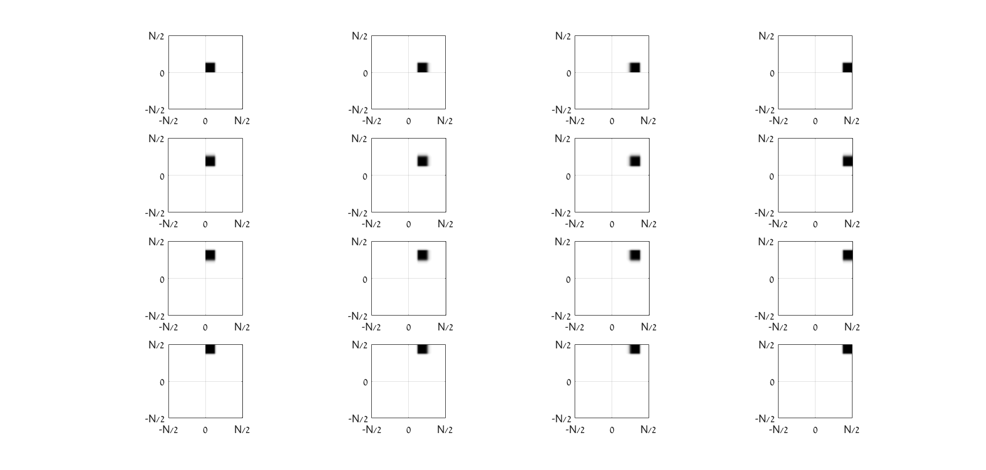
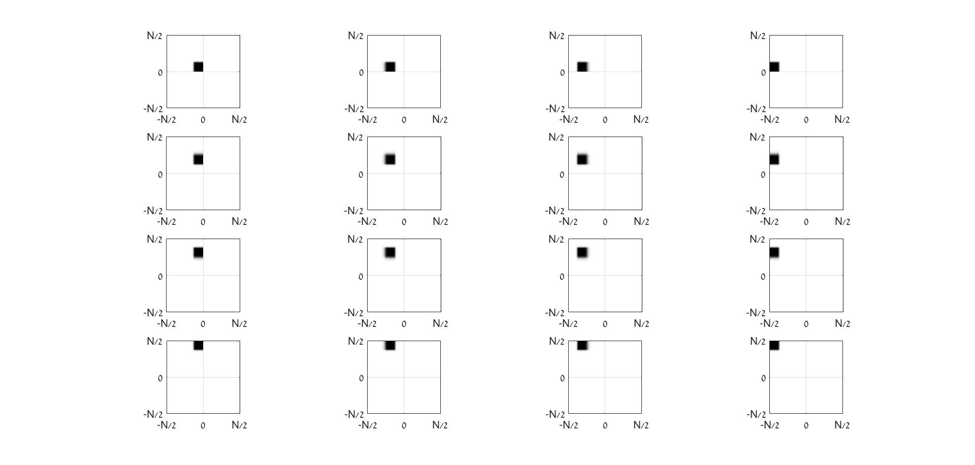
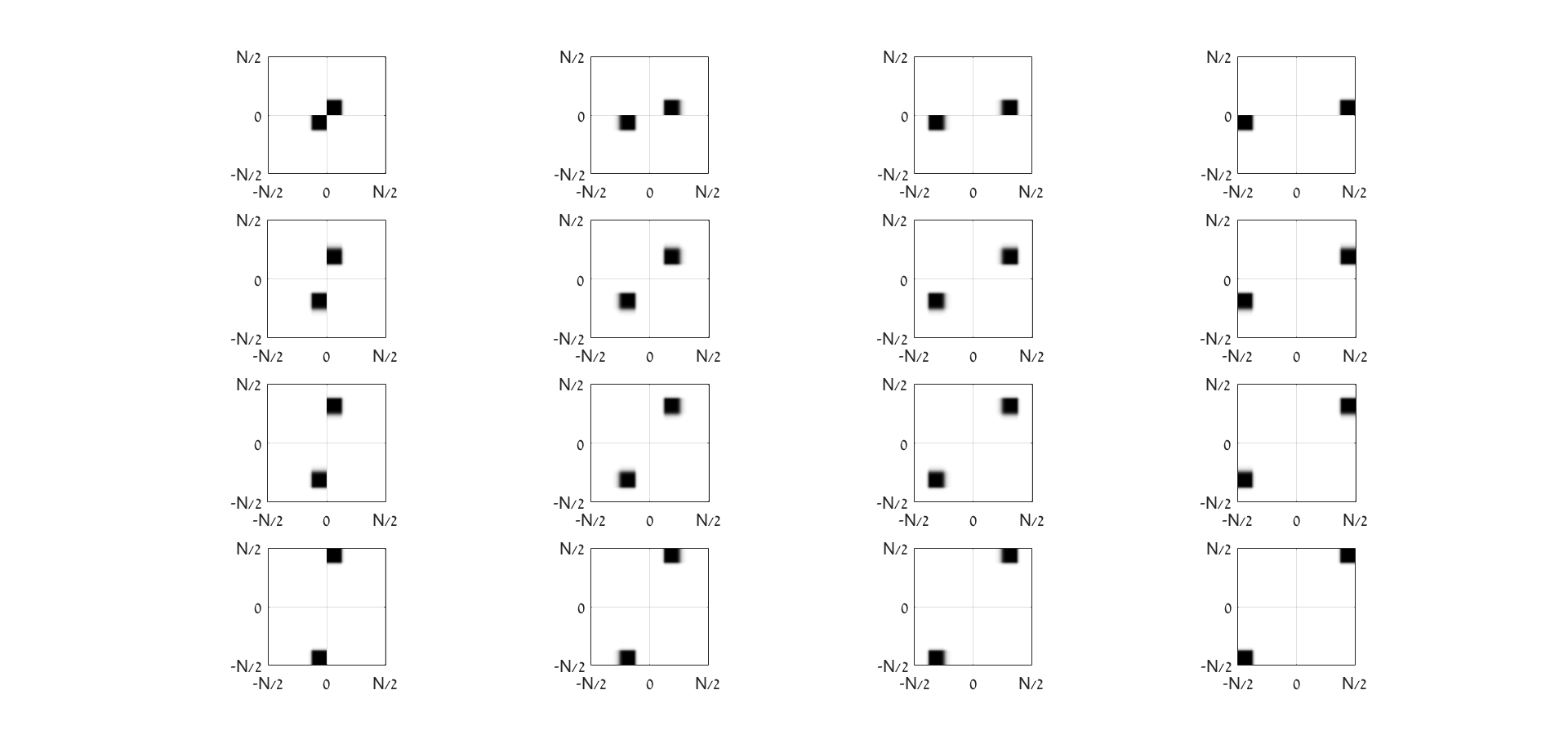
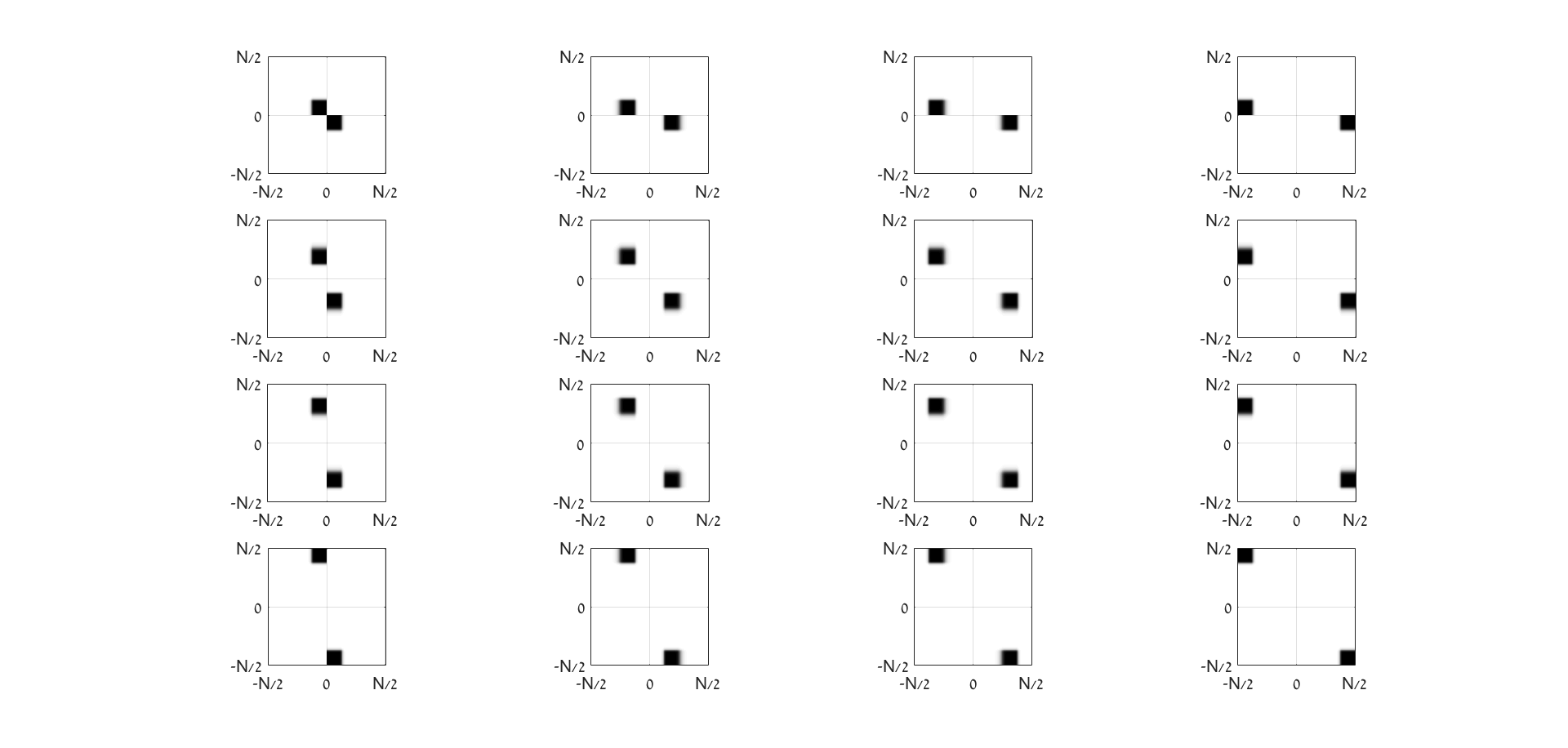
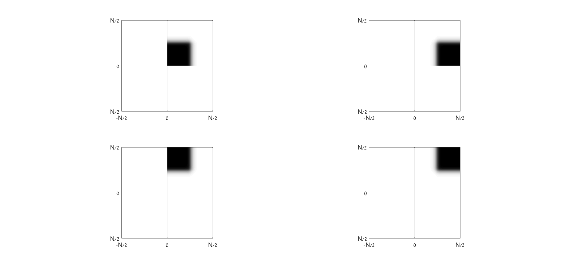
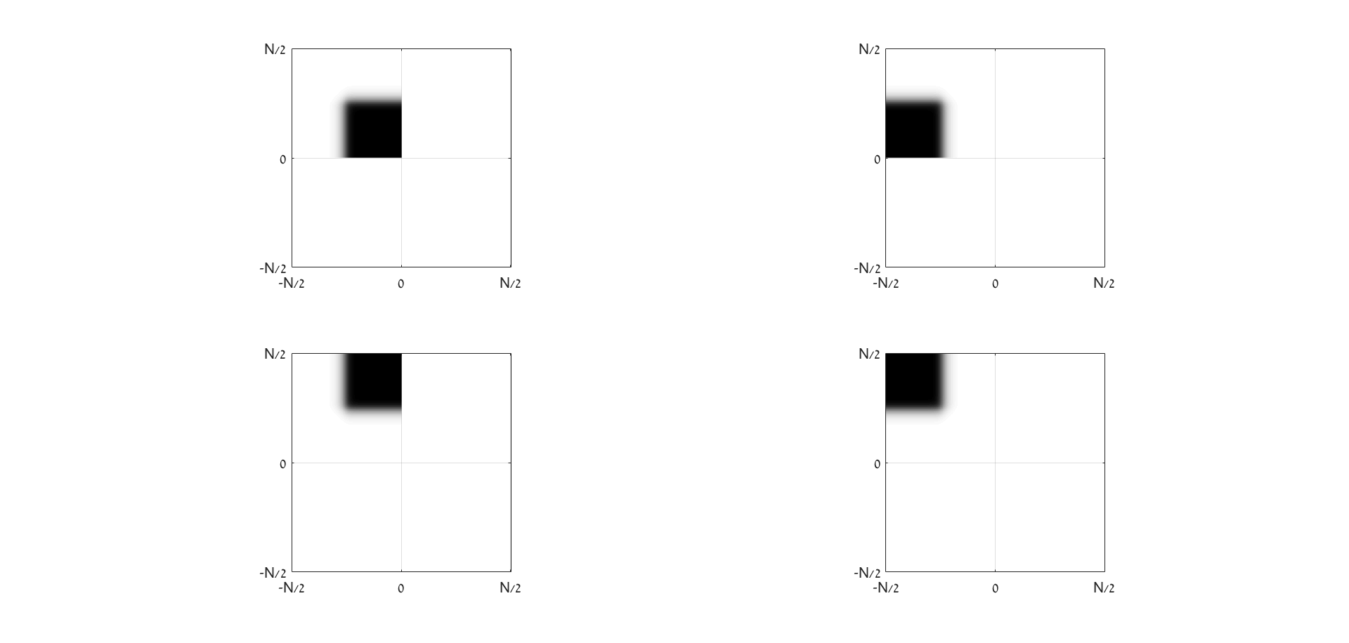
and, as such, they fill the quadrant of the frequency domain, while the spectra of fill the quadrant . Figures 5.1 and 5.2 display the magnitude spectra of the tenth-order 2D qWPs and from the second decomposition level, respectively.
Remark 5.1
The 2D qWPs are the tensor products of 1D qWPs from the decomposition level . However, there is no problems to design the 2D qWPs as a tensor products of 1D qWPs from different decomposition levels such as
5.1.2 Directionality of real-valued 2D WPs
It is seen in Fig. 5.1 that the DFT spectra of the qWPs effectively occupy relatively small squares in the frequency domain. For deeper decomposition levels, sizes of the corresponding squares decrease on geometric progression. Such configurations of the spectra lead to the directionality of the real-valued 2D WPs and .
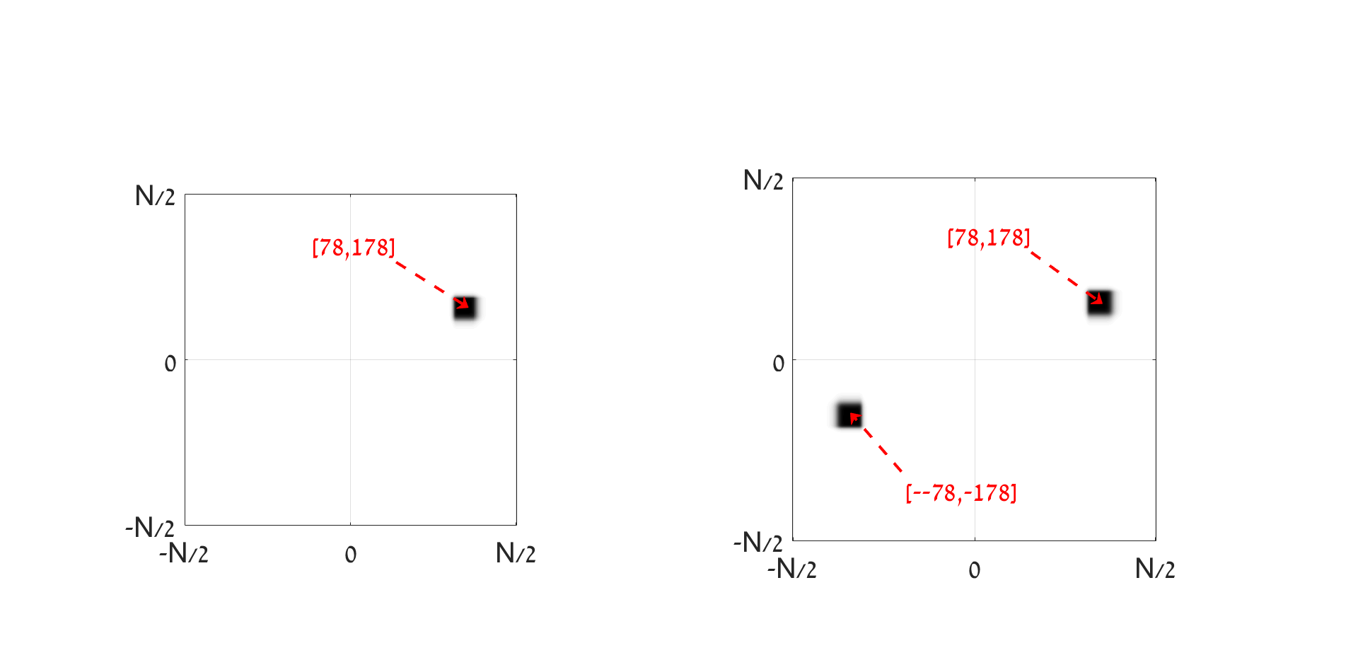
Assume, for example, that and denote and . Its magnitude spectrum , displayed in Fig, 5.3, effectively occupies the square of size pixels centered around the point , where . Thus, the WP is represented by
Consequently, the real-valued WP is represented as follows:
The spectrum of the 2D signal comprises only f low frequencies in both directions and the signal does not have a directionality. But the 2D signal is oscillating in the direction of the vector . The 2D WP is well localized in the spatial domain as is seen from Eq. (5.1) and the same is true for the low-frequency signal . Therefore, WP can be regarded as the directional cosine modulated by the localized low-frequency signal .
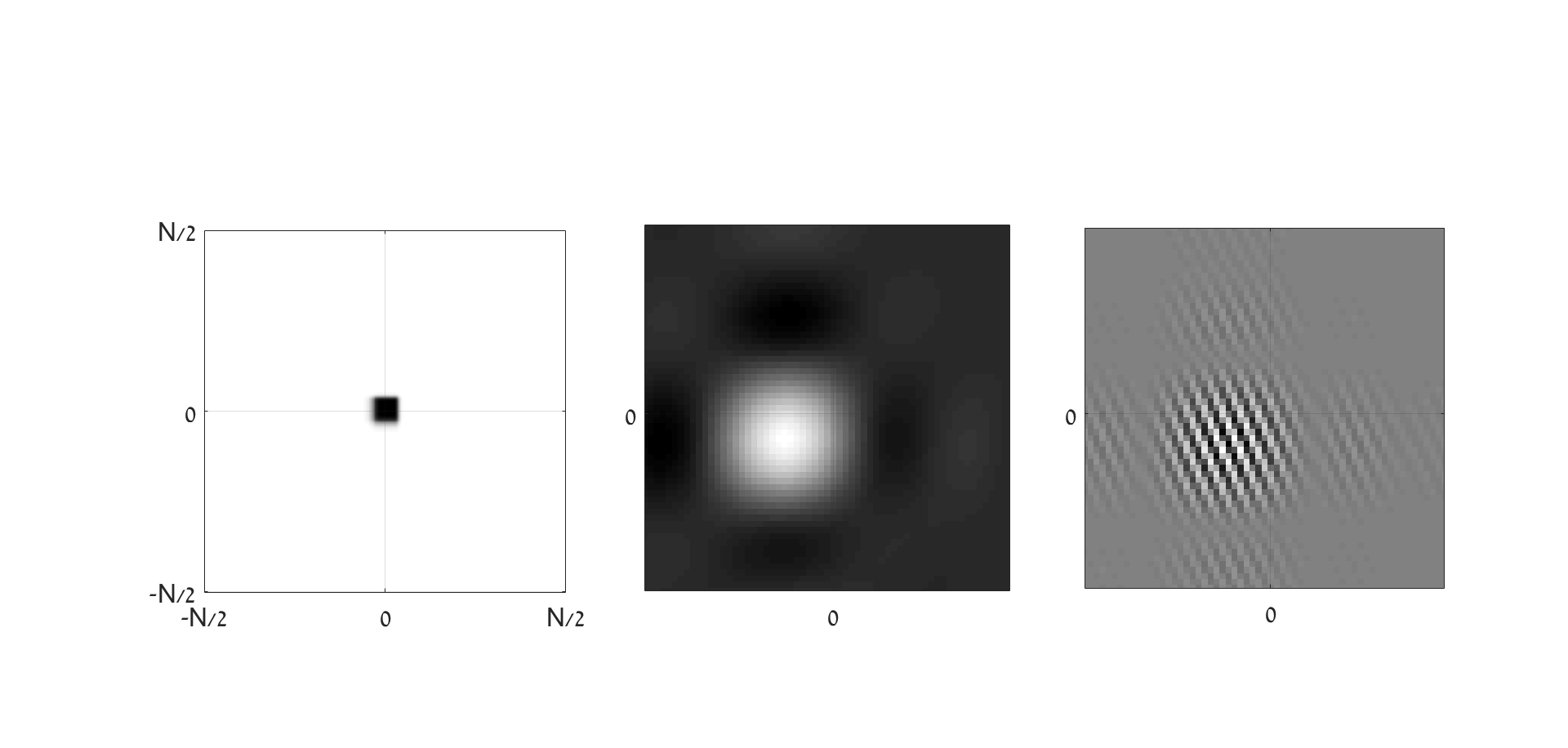
The same arguments, which to some extent are similar to the discussion in Section 6.2 of [10], are applicable to all four real-valued 2D WPs defined in Eqs. (5.1) – (5.2). Figure 5.4 displays the low-frequency signal , its magnitude spectrum and the 2D WP .
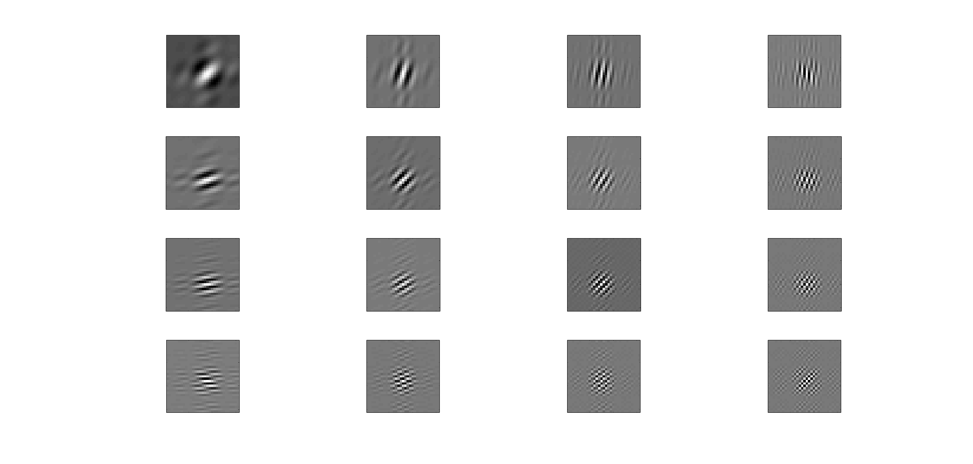
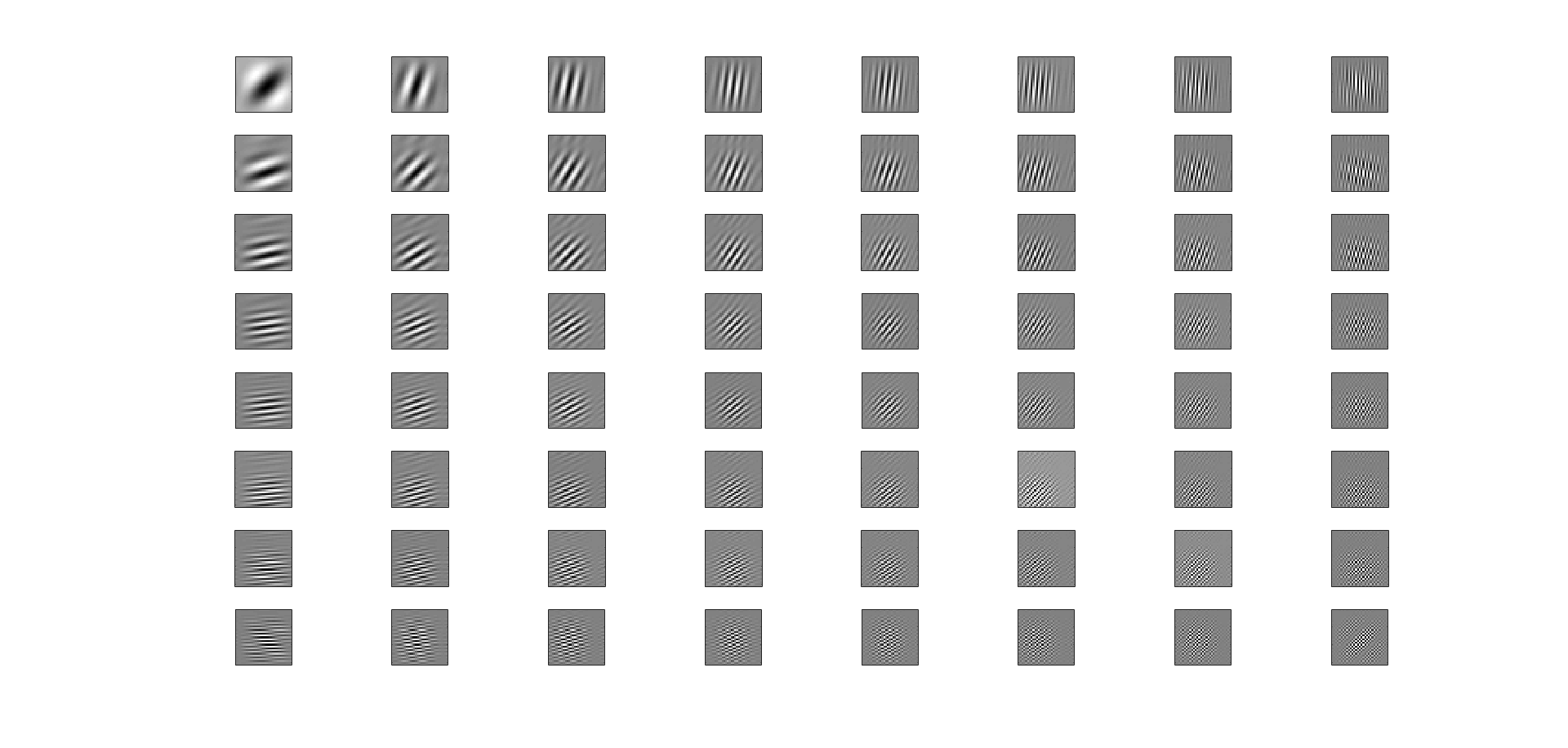
Figures 5.5 and 5.6 display WPs from the second decomposition level and their magnitude spectra, respectively. Figures 5.7 and 5.8 display WPs from the second decomposition level and their magnitude spectra, respectively.

Remark 5.2
Note that orientations of the vectors and are approximately the same. These vectors determine the orientations of the WPs and , respectively. Thus, these WPs have approximately the same orientation. Consequently, the WPs from the -th decomposition level are oriented in different directions. The same is true for the WPs . Thus, altogether, at the level we have WPs oriented in different directions. It is seen in Figs. 5.5, 5.7 and in Figs. 5.9, 5.10 that display the WPs .

6 Implementation of 2D qWP transforms
The spectra of 1D qWPs , fill the non-negative half-band , and vice versa for the qWPs . Therefore, the spectra of 2D qWPs fill the quadrant of the frequency domain, while the spectra of 2D qWPs fill the quadrant . It is clearly seen in Fig. 6.1.
Consequently, the spectra of the real-valued 2D WPs , and fill the pairs of quadrant and , respectively (Figs. 5.6 and 5.8).
By this reason, none linear combination of the WPs and their shifts can serve as a basis in the signal space . The same is true for WPs . However, combinations of the WPs provide frames of the space .
6.1 One-level 2D transforms
The one-level 2D qWP transforms of a signal are implemented by a tensor-product scheme mentioned in Section 2.5.
6.1.1 Direct transforms with qWPs
Denote by the 1D transforms of row signals from with the analysis modulation matrices which are defined in Eq. (4.6). Application of these transforms to rows of a signal X produces the coefficient arrays
Denote by the 1D inverse transforms with the synthesis modulation matrices . Due to Proposition 4.2, application of these transforms to rows of the coefficient arrays , respectively, produces the 2D analytic signals:
| (6.1) |
where H(X) is the 2D signal consisting of the HTs of rows of the signal X.
Denote by the direct 1D transform determined by the modulation matrix applicable to columns of the corresponding signals. The next step of the tensor product transform consists of the application of the 1D transform to columns of the arrays As a result, we get four transform coefficients arrays:
Hence, it follows that
| (6.3) |
Remark 6.1
Recall that the DFT spectra of WPs and which are the real and imaginary parts of the qWP , are confined within the area of the frequency domain. It is seen from Eq. (6.3) that if at least a part of the spectrum of a signal is located in the area , then the signal cannot be fully restored from the transform coefficients , although their number is the same as the number of samples in the signal . To achieve a perfect reconstruction, the coefficients from the arrays should be incorporated.
The coefficient arrays are derived in the same way as the arrays . The only difference is that, for the 1D transform the modulation matrix is used instead of . For the transform , the modulation matrix is used. Consequently, to derive the coefficient arrays , the transform should be applied to columns of the arrays . As a result, we get
6.1.2 Inverse transforms with qWPs
Denote by the 1D inverse transform with the synthesis modulation matrix applicable to columns of the coefficient arrays. Denote by the HTs of the arrays consisting of columns of the coefficient arrays . Proposition 4.2 implies that
where and are analytic coefficient arrays. Denote by a signal from such that
| (6.5) |
Equations (6.1) and (6.5) imply that the applications of the transforms to rows of the respective coefficient arrays results in the following relations:
| (6.6) | |||||
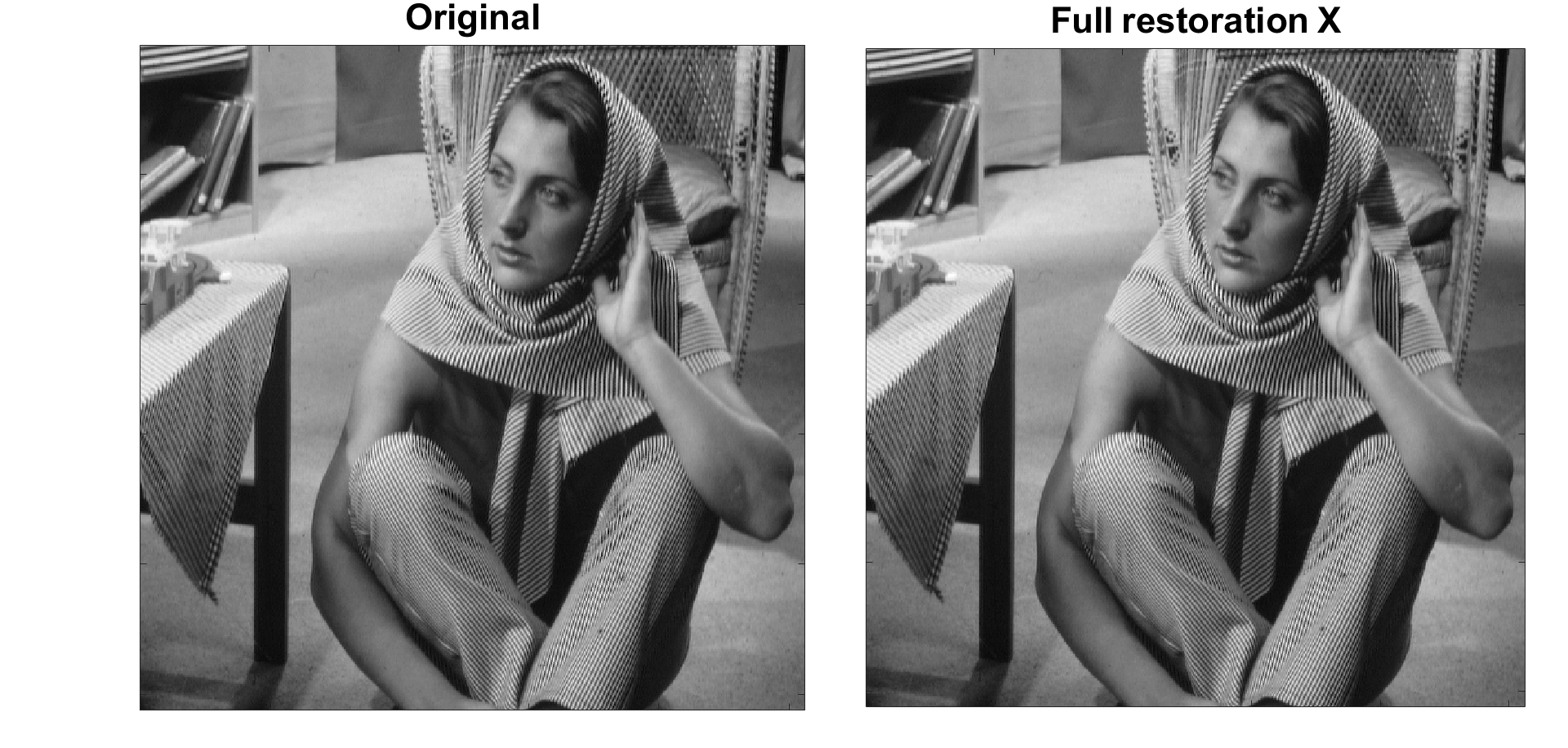
Finally, we have the signal X restored by .
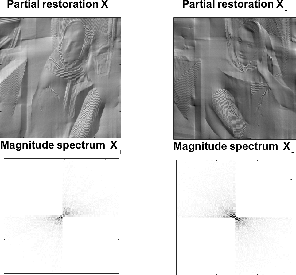
Figures 6.2 and 6.3 illustrate the image “Barbara” restoration by the 2D signals and . The signal captures edges oriented to north-east, while captures edges oriented to north-west. The signal perfectly restores the image achieving PSNR=313.8596 dB.
6.2 Multi-level 2D transforms
It was established in Section 4.2 that the 1D qWP transforms of a signal to the second and further decomposition levels are implemented by the iterated application of the filter banks, that are determined by their analysis modulation matrices to the coefficients arrays . The transforms applied to the arrays produce the arrays , respectively. The inverse transform consists of the iterated application of the filter banks that are determined by their synthesis modulation matrices to the coefficients arrays . In that way the first-level coefficient arrays are restored.
The tensor-product of the 2D transforms of a signal consists of the subsequent application of the 1D transforms to columns and rows of the signal and coefficients arrays. By application of filter banks, which are determined by the analysis modulation matrix to columns and rows of coefficients array , we derive four second-level arrays . The arrays are restored by the application of the filter banks that are determined by their synthesis modulation matrices to rows and columns of the coefficients arrays . The transition from the second to further levels and back are executed similarly using the modulation matrices and , respectively. The inverse transforms produce the coefficients arrays from which the signal is restored using the synthesis modulation matrices as it is explained in Section 6.1.2.
All the computations are implemented in the frequency domain using the FFT. For example, the Matlab execution of the 2D qWP transform of a image down to the sixth decomposition level takes 1.34 seconds. The four-level transform takes 0.28 second.
Summary
The 2D qWP processing of a signal is implemented by a dual-tree scheme. The first step produces two sets of the coefficients arrays: which are derived using the analysis modulation matrix , and which are derived using the analysis modulation matrix . Further decomposition steps are implemented in parallel on the sets and using the same analysis modulation matrix , thus producing two multi-level sets of the coefficients arrays and .
By parallel implementation of the inverse transforms on the coefficients from the sets and using the same synthesis modulation matrix , the sets and are restored, which, in turn, provide the signals and , using the synthesis modulation matrices and , respectively. Typical signals and their DFT spectra are displayed in Fig. 6.2.
Prior to the reconstruction, some structures, possibly different, are defined in the sets and (2D wavelet or Best Basis structures, for example) and some manipulations on the coefficients, (thresholding, minimization, for example) are executed.
7 Numerical examples
In this section, we present two examples of application of the 2D qWPs to image restoration. These examples illustrate the ability of the qWPs to restore edges and texture details even from severely damaged images. Certainly, this ability stems from the fact that the designed 2D qWP transforms provide a variety of 2D waveforms oriented in multiple directions, from perfect frequency resolution of these waveforms and, last but not least, from oscillatory structure of many waveforms.
7.1 Denoising examples
An image is represented by the 2D signal . The image, which is corrupted by additive Gaussian noise with STD=, is represented by the 2D signal . We apply the following image denoising scheme:
-
•
2D transform of the signal with directional qWPs and down to level is implemented to generate two sets of the coefficients arrays and .
-
•
For comparison, the 2D WP transform of the signal with non-directional WP down to level is implemented thus generating the set of the coefficients arrays.
-
•
In each of the sets and the “Best Basis” is selected by a standard procedure of comparison the cost function (entropy or norm) of the “parent” coefficients block with the cost functions of its “offsprings” (see [7]). The selected bases are designated by and , respectively.
-
•
The number of the transform coefficients and associated with each basis is the same as the number of pixels in the image.
-
•
Denoising of the signal is implemented by hard thresholding of the coefficients and .
-
•
The thresholds for the coefficients arrays are defined by the following naive scheme:
-
1.
The absolute values of the coefficients from each set and are arranged in an ascending order thus forming the sequences and , respectively.
-
2.
The values of the -th term and are selected as the thresholds for the coefficients arrays and , respectively. The number is chosen depending on the noise intensity.
-
1.
-
•
The sets of the transform coefficients and are subjected to thresholding with the selected values and , respectively, and, after that the inverse transforms are applied to produce the 2D signals from the directional qWPT and from the non-directional tensor product WPT.
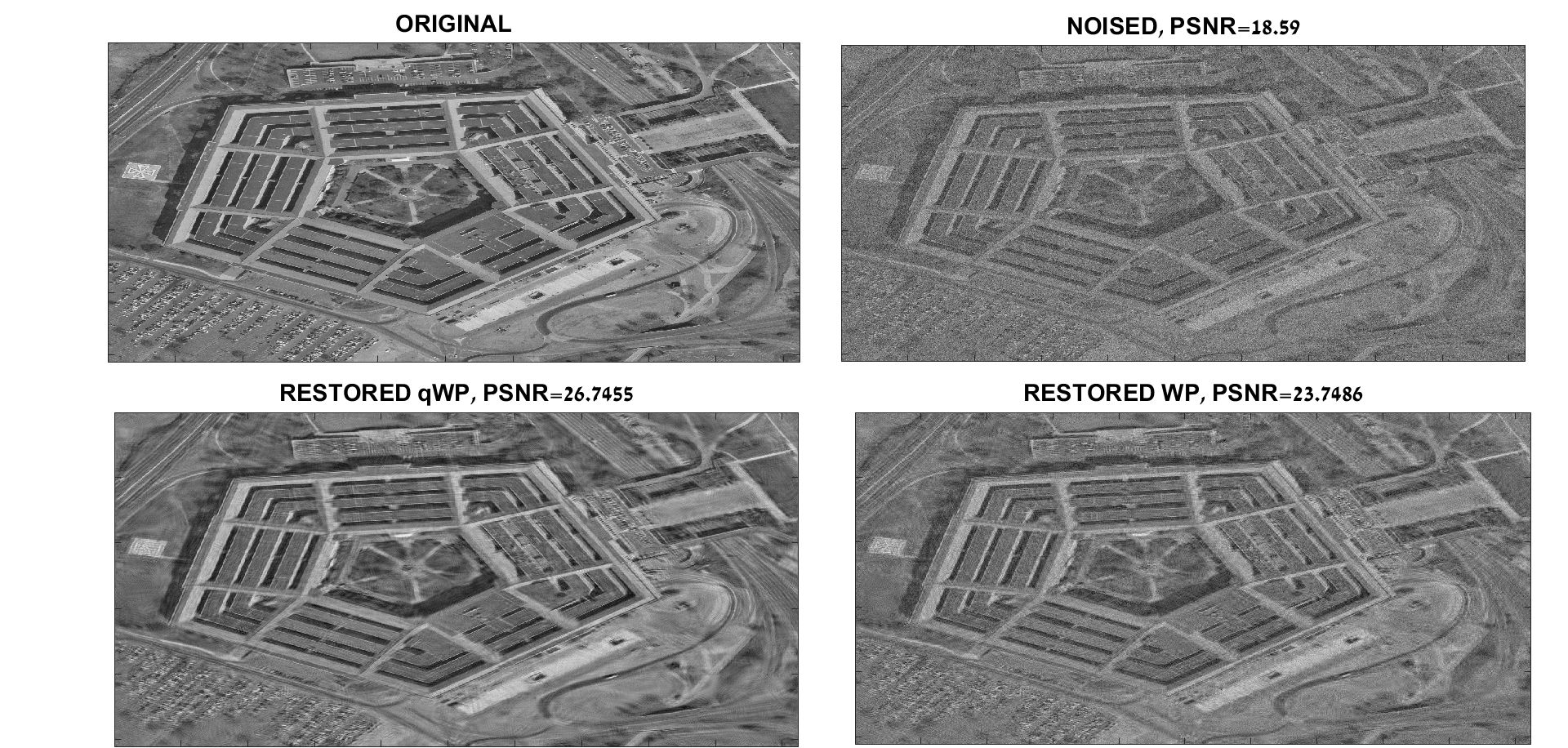
7.1.1 Example I: “Pentagon” image
The “Pentagon” image of size (1048576 pixels) was corrupted by additive Gaussian noise with STD=30 dB. As a result, the PSNR of the corrupted image was 18.59 dB. The corrupted image was decomposed by the directional qWPs and originating from the fourth-order discrete splines down to a fourth decomposition level. In this way, two sets and , of the transform coefficients were produced. For comparison, the corrupted image was decomposed by the non-directional WPs , which resulted in the set of the coefficients arrays.
The “Best Bases” and were designed for the coefficient arrays. The thresholds and were selected for each set of the coefficient arrays. was chosen. Thus, we had , and .
Remark 7.1
The threshold is approximately two times less than the threshold . It happens because the transform coefficients are complex-valued and the threshold is operating with absolute values of the coefficients.
Remark 7.2
qWPs oriented in 62 different directions were involved. The Matlab implementation of all the above procedures takes 4.2 seconds.
Figure 7.1 is the outputs of the image reconstruction by the directional qWPT and the non-directional tensor product WPT from the thresholded coefficients arrays. The qWPT-restored image image has PSNR=26.75 dB versus PSNR=23.75 dB for the WPT-restored image . Visually, image is cleaner in comparison to and more fine details are restored.
7.1.2 Example II: “Barbara” image
We present two cases with the “Barbara” image. In one case, the image was corrupted by an additive Gaussian noise with STD=30 dB and in the other, the noise was more intensive with STD=50 dB.
- Noise with STD=30 dB:
-
In this case, the PSNR of the corrupted image was 18.59 dB. In order to avoid boundary effects, the image of size was symmetrally extended to the size . After processing, the results were shrunk to the original size. The corrupted image was decomposed by the directional qWPs and originating from the fourth-order discrete splines down to third decomposition level. In this way, the two sets and , of the transform coefficients were produced. For comparison, the corrupted image was decomposed by the non-directional WPs , which resulted in the set of the coefficients arrays.
The “Best Bases” and were designed for the coefficient arrays. The thresholds and were selected for each set of the coefficient arrays. was chosen. Thus, we had , and .
Figures 7.2 and 7.3 are the outputs of the image reconstruction by using the directional qWPT and the non-directional tensor product WPT from the thresholded coefficients arrays. The qWPT-restored image has PSNR=28.52 dB versus PSNR=25.20 dB for the WPT-restored image . Visually, the image is much cleaner in comparison to and almost all edges and the texture structure are restored.
Remark 7.3
qWPs oriented in 31 different directions are involved. In this case, the image under processing has four times more pixels than the original image. The Matlab implementation of all the procedures including 3-level qWP and WP transforms, design of “Best Bases”, thresholding of the coefficients arrays and the inverse transforms takes 3.5 seconds. Processing the image without the extension takes 0,88 seconds and produces the restores image with PSNR=28.32 dB.
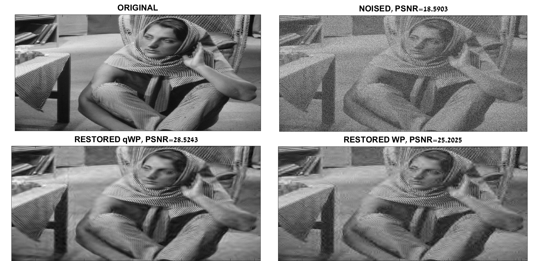
Figure 7.2: Top left: Original “Barbara” image. Top right: Image corrupted by noise with STD=30 dB. Bottom left: The qWPT-based restored image . Bottom right: WPT-based restored image 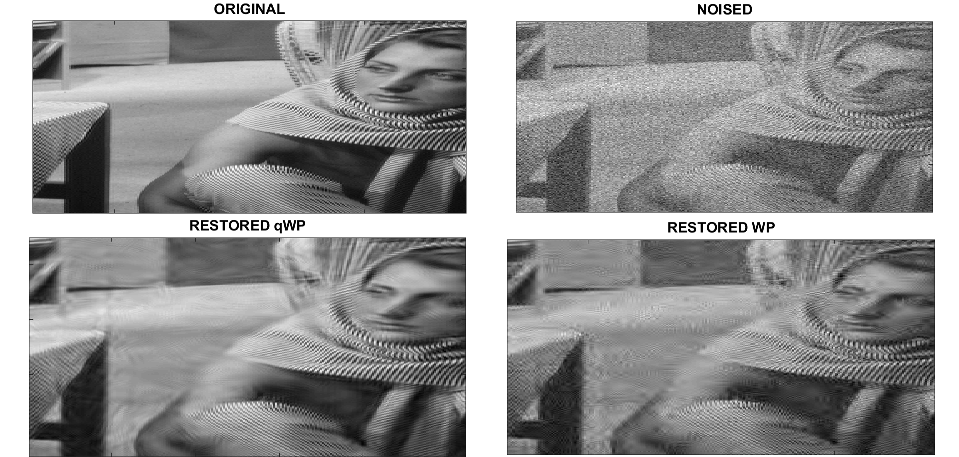
Figure 7.3: Fragments of the images shown in Fig. 7.2 - Noise with STD=50 dB:
-
In this case, the PSNR of the corrupted image was 14.14 dB. The same operations as in the previous case were applied to the corrupted image. was chosen. Thus, we had , and .
Figures 7.4 and 7.5 are the outputs of the image reconstruction by using the directional qWPT and the non-directional tensor product WPT from the thresholded coefficients arrays. The qWPT-based restored image has PSNR=25.66 dB versus PSNR=22.20 dB for the WPT-based restored image . Visually, the image is cleaner in comparison to , which, in addition comprises many artifacts. Many edges and the texture structure are retained in the image .
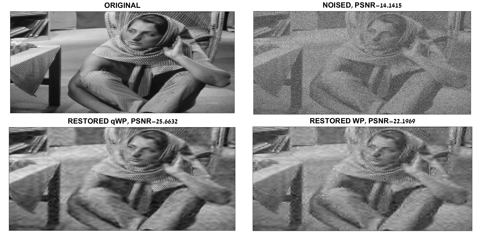
Figure 7.4: Top left: Original “Barbara” image. Top right: Image corrupted by noise with STD=50 dB. Bottom left: The qWPT-based restored image . Bottom right: WPT-based restored image 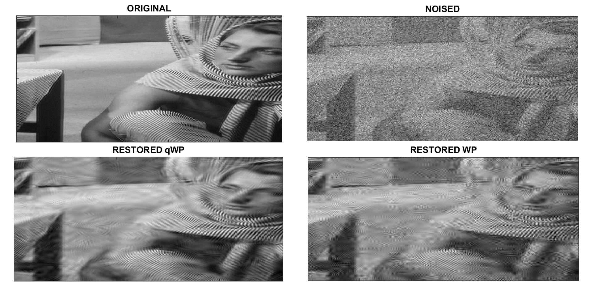
Figure 7.5: Fragments of the images shown in Fig. 7.4 Comment
7.2 Image restoration examples
In this section we present a few cases of image restoration using directional qWPs. Images to be restored were degraded by blurring, aggravated by random noise and random loss of significant number of pixels. In our previous work ([1] and Chapter 18 in [4]) we developed the image restoration scheme utilizing 2D wavelet frames designed in Chapter 18 of [4]. In the examples presented below we use, generally, the same scheme as in [4] with the difference that the directional qWPs designed in Section 6 are used instead of wavelet frames.
7.2.1 Brief outline of the restoration scheme
Images are restored by the application of the split Bregman iteration (SBI) scheme [8] that uses the so-called analysis-based approach (see for example [16]).
Denote by the original image array to be restored from the degraded array where denotes the operator of 2D discrete convolution of the array with a kernel , and is the random error array. denotes the conjugate operator of , which implements the discrete convolution with the transposed kernel . If some number of pixels are missing then the image should be restored from the available data
| (7.1) |
where denotes the projection on the remaining set of pixels.
The solution scheme is based on the assumption that the original image can be sparsely represented in the qWP domain. Denote by the operator of qWP expansion of the image . To be specific, the 2D transform of the signal with directional qWP and down to level is implemented to generate two sets of the coefficients arrays and . In each of the sets either “Best Basis” or “basis”, which consist of shifts of all the WPs from the decomposition level , are selected. The bases are designated by . The number of the transform coefficients associated with each basis is the same as the number of pixels in the image. Thus, is the set of the transform coefficients.
Denote by the reconstruction operator of the image from the set of the transform coefficients. We get , , where is the identity operator.
An approximate solution to Eq. (7.1) is derived via minimization of the functional
| (7.2) |
where and are the and the norms of the sequences, respectively. If , then
Denote by the operator of soft thresholding:
Following [16], we solve the minimization problem in Eq. (7.2) by an iterative SBI algorithm. We begin with the initialization . Then,
| (7.3) |
The linear system in the first line of Eq. (7.3) is solved by the application of the conjugate gradient algorithm. The operations in the second and third lines are straightforward. The choice of the parameters and depends on experimental conditions.
7.2.2 Examples
- Example I: “Barbara” blurred, missing 50% of pixels:
-
The “Barbara” image was restored after it was blurred by a convolution with the Gaussian kernel (MATLAB function
fspecial(’gaussian’,[5 5])) and its PSNR became 23.32 dB. Then, 50% of its pixels were randomly removed. This reduced the PSNR to 7.56 dB. Random noise was not added. The image was restored by 50 SBI using the parameters in Eq. (7.3). The conjugate gradient solver used 150 iterations. qWPs originating from discrete splines of sixth order were used. For “bases”, 8-samples shifts of all the WPs from the third decomposition level were selected. Matlab implementation of the restoration procedures took 59.6 seconds.Figure 7.6 displays the restoration result. The image is deblurred and the fine texture is restored completely with PSNR=32.09 dB. Note that the best result in an identical experiment reported in [4] achieved PSNR=30.32 dB.
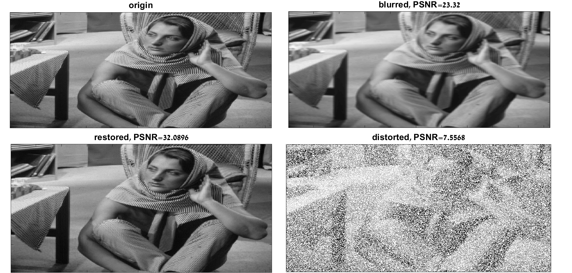
Figure 7.6: Top left: Source input - “Barbara” image. Top right: Blurred, PSNR=23.32 dB. Bottom right: After random removal of 50% of its pixels. PSNR=7.56 dB. Bottom left: The image restored by the directional qWPT. PSNR=32.09 dB - Example II: “Barbara” blurred, added noise, missing 50% of pixels:
-
The “Barbara” image was restored after it was blurred by a convolution with the Gaussian kernel (MATLAB function fspecial(’gaussian’,[5 5])). Random Gaussian noise with STD=10 dB was added and the image PSNR became 22.08 dB. Then, 50% of its pixels were randomly removed. This reduced the PSNR to 7.53 dB. The image was restored by 70 SBI using the parameters in Eq. (7.3). The conjugate gradient solver used 15 iterations. qWPs originating from discrete splines of fourth order were used. For the “bases”, 16-samples shifts of all the WPs from the fourth decomposition level were selected. Matlab implementation of the restoration procedures took 51.9 seconds.
Figure 7.7 displays the restoration result. The image is deblurred, noise is removed and the fine texture is partially restored producing PSNR=24.31 dB. Note that the best result in an identical experiment reported in [4] achieved PSNR=24.19 dB.
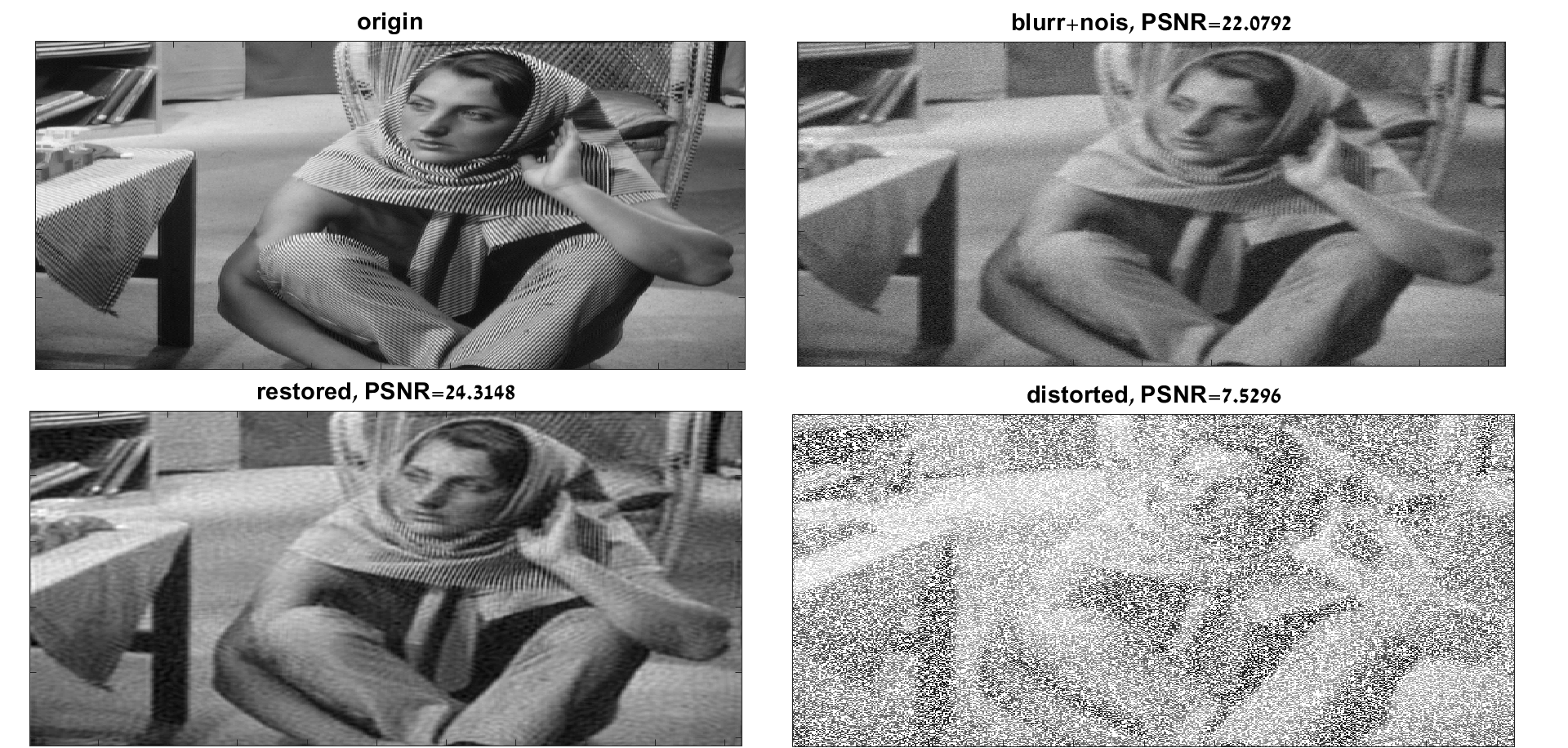
Figure 7.7: Top left: Source input - “Barbara” image. Top right: Blurred and noised, PSNR=22.08 dB. Bottom right: After random removal of 50% of its pixels. PSNR=7.53 dB. Bottom left: The restored image by the directional qWPT. PSNR=24.31 dB - Example III: “Barbara” blurred, missing 90% of pixels:
-
The “Barbara” image was restored after it was blurred by a convolution with the Gaussian kernel (MATLAB function
fspecial(’gaussian’,[5 5])) and 90% of its pixels were randomly removed. This reduced the PSNR to 5.05 dB. The image was restored by 150 SBI using the parameters in Eq. (7.3). The conjugate gradient solver used 150 iterations. qWPs originating from discrete splines of eighth order were used. For the “bases”, 16-samples shifts of all the WPs from the fourth decomposition level were selected. Matlab implementation of the restoration procedures took 226.8 seconds.Figure 7.8 displays the restoration result. The image is deblurred and the fine texture is partially restored. The output has PSNR=25.24 dB.
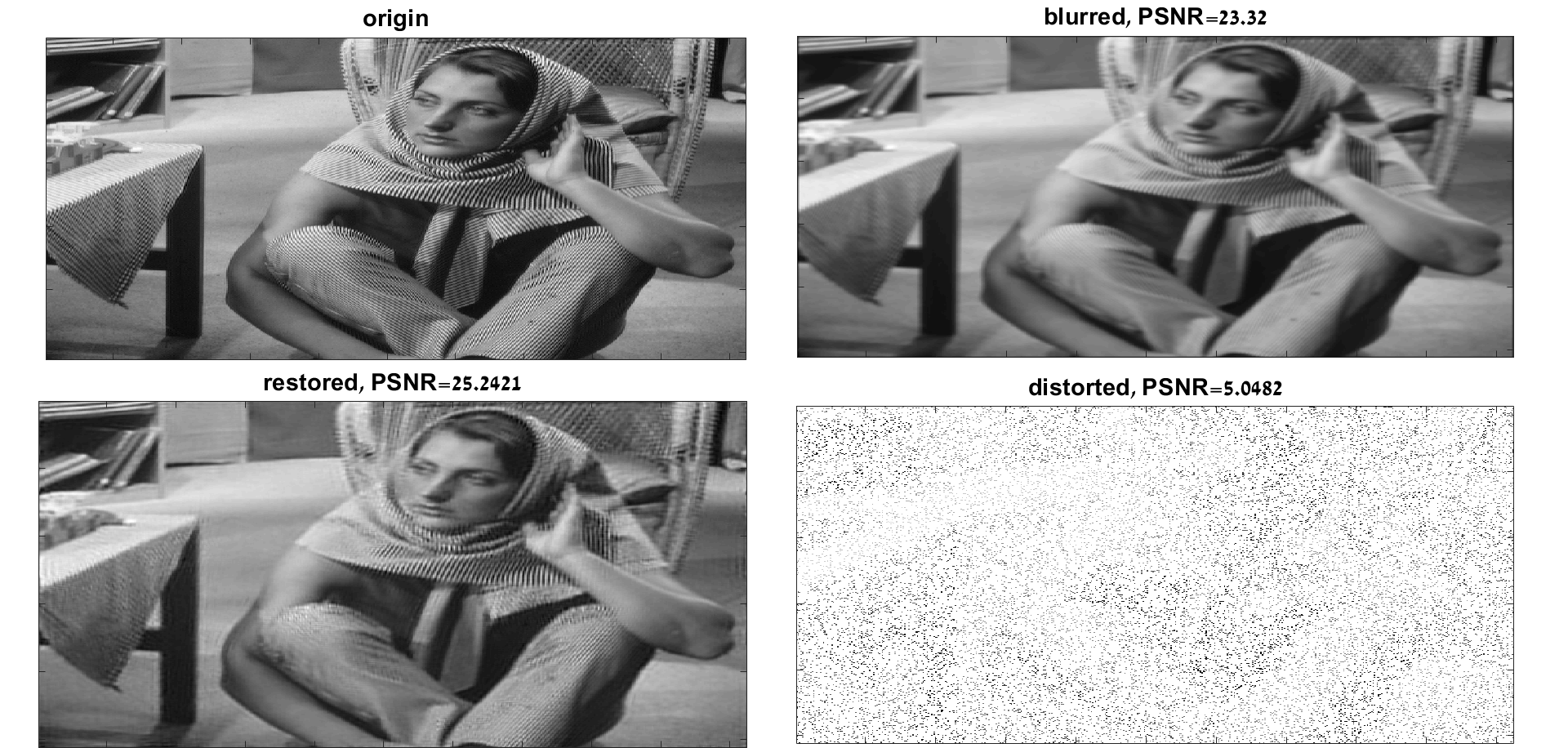
Figure 7.8: Top left: Source input - “Barbara” image. Top right: Blurred, PSNR=23.32 dB. Bottom right: After random removal of 90% of its pixels. PSNR=5.05 dB. Bottom left: The image restored by the directional qWPT. PSNR=25.24 dB
8 Discussion
We presented a library of complex discrete-time wavelet packets operating in one- or two-dimensional spaces of periodic signals. Seemingly, the requirement of periodicity imposes some limitations on the scope of signals available for processing, but actually these limitations are easily circumvented. Any limited signal can be regarded as one period of a periodic signal. In order to prevent boundary effects, the signals can be symmetrally extended beyond the boundaries before processing and shrunk to the original size after that. We used such a trick in the “Barbara” denoising examples.
On the other hand, the periodic setting provides a lot of substantial opportunities for the design and implementation of WP transforms such as
-
•
A unified computational scheme based on 1D and 2D FFT.
-
•
Opportunity to use filters with infinite impulse responses, which enables us to design a variety of orthonormal WP systems where WPs can have any number of local vanishing moments.
-
•
The number of local vanishing moments does not affect the computational cost of the transforms implementation.
-
•
A simple explicit scheme of expansion of real WPs to analytic and quasi-analytic WPs with perfect frequency separation.
The library of qWP transforms described in the paper has a number of free parameters enabling to adapt the transforms to the problem under consideration:
-
•
Order of the generating spline, which determines the number of local vanishing moments.
-
•
Depth of decomposition, which in 2D case determines the directionality of qWPs. For example, fourth-level qWPs are oriented in 62 different directions.
-
•
Selection of an optimal structure, such as, for example, separate Best Bases in the real and imaginary parts of 1D qWP transforms, separate “Best Bases” in positive and negative branches of 2D dual-tree qWP transforms, a wavelet-basis structure or the set of all wavelet packets from a single level.
-
•
Controllable redundancy rate of the signal representation. The minimal rate is 2 when one of options listed in a previous item is utilized. However, several basis-type structures can be involved, for example, all wavelet packets from several levels can be used for the signal reconstruction and results can be averaged.
The goal of the paper is to design qWPs with an efficient computational scheme for the corresponding transforms. A few experimental results highlight exceptional properties of these WPs. The directional qWPs are tested for image restoration examples. In the denoising examples, the goal was not to achieve the best output in RSNR values but rather to compare the performance of directional versus standard WPs that are tensor-product-based. We did not use sophisticated adaptive denoising schemes such as for example Gaussian scale mixture model ([21]) or bivariate shrinkage ([25]). Instead, after decomposition of an image down to level , we selected “Best Bases” in the positive and negative branches of the qWP transform and in the WP transform. Then, we discarded all the coefficients in these bases except for the largest coefficients. Even with such naive scheme, the directional qWPs significantly outperform the standard WPs in both PSNR values and in the visual perception. The edges, lines and oscillating texture structures in the “Barbara” image, which was corrupted by Gaussian noise with STD=30 dB, were almost perfectly restored. When noise STD was 50 dB, an essential part of these structures was restored as well. We emphasise that the Matlab implementation of all the procedures including 3-level qWP and WP transforms, the design of “Best Bases”, thresholding of the coefficients arrays and inverse transforms took 0.88 seconds. To eliminate boundary effects, the image was extended from to and the processing took 3.5 seconds.
The second group of experimental results dealt with the restoration of the “Barbara” image which was blurred my the convolving the image with a Gaussian kernel and degraded by removing randomly either 50% or 90% of the pixels. The image was restored by using a constrained minimization of the qWP transform coefficients from a certain decomposition level and implemented via the split Bregman Iterations procedure. In Example I with missing 50% of the pixels, the image was almost perfectly restored with PSNR-32.1 dB and practically all the fine structure reconstructed although it was blurred even before the removal of the pixels. Addition of the Gaussian noise with STD 10 dB to the blurred image in Example II depleted the reconstruction result. Although the noise became suppressed and the image was deblurred, most of the fine structure was lost. Restoration results were better in Example III where, instead of adding noise, the number of pixels missing from the blurred image was raised to 90%. The image was deblurred and an essential part of fine structure was restored.
Summarizing, we can state that, having such a versatile and flexible tool at hand, we are prepared to address multiple data processing problems such as signal and image deblurring and denoising, target detection, segmentation, inpainting, superresolution, to name a few. In one of the applications, whose results are to be published soon, directional qWPs are used with Compressed Sensing methodology for the conversion of a regular digital photo camera to an hyperspectral imager. Preliminary results appear in [9]. Special efforts are on the way for the design of a denoising scheme which fully explores the directionality properties of qWPs.
Acknowledgment
This research was partially supported by the Israel Science Foundation (ISF, 1556/17), Blavatnik Computer Science Research Fund Israel Ministry of Science and Technology 3-13601 and by Academy of Finland (grant 311514).
References
- [1] A. Averbuch, P. Neittaanmäki, and V. Zheludev. Periodic spline-based frames: Design and applications for image restoration. Inverse Problems and Imaging, 9(3):661–707, 2015.
- [2] A. Averbuch, P. Neittaanmäki, and V. Zheludev. Splines and spline wavelet methods with application to signal and image processing, Volume III: Selected topics. Springer, 2019.
- [3] A. Averbuch, V. Zheludev, and M. Khazanovsky. Deconvolution by matching pursuit using spline wavelet packets dictionaries. Appl. Comput. Harmon. Anal., 31(1):98–124, 2011.
- [4] A. Z. Averbuch, P. Neittaanmäki, and V. A. Zheludev. Spline and spline wavelet methods with applications to signal and image processing, Volume I: Periodic splines. Springer, 2014.
- [5] I. Bayram and I. W. Selesnick. On the dual-tree complex wavelet packet and m-band transforms. IEEE Trans. Signal Process., 56, 2008.
- [6] Z. Che and X. Zhuang. Digital affine shear filter banks with 2-layer structure and their applications in image processing. IEEE Transactions on Image Processing, 27(8):3931–3941, 2016.
- [7] R. R. Coifman and V. M. Wickerhauser. Entropy-based algorithms for best basis selection. IEEE Trans. Inform. Theory, 38(2):713–718, 1992.
- [8] T. Goldstein and S. Osher. The split Bregman method for -regularized problems. SIAM J. Imaging Sci., 2(2):323–343, 2009.
- [9] M. Golub, A. Averbuch, M. Nathan, V. Zheludev, J. Hauser, S. Gurevitch, R. Malinsky, and A. Kagan. Compressed sensing snapshot spectral imaging by a regular digital camera with an added optical diffuser. Applied Optics, 55:432–443, March 2016.
- [10] B. Han and Z. Zhao. Tensor product complex tight framelets with increasing directionality. SIAM J. Imaging Sci., 7, 2014.
- [11] B. Han, Z. Zhao, and X. Zhuang. Directional tensor product complex tight framelets with low redundancy. Appl. Comput. Harmon. Anal., 41(2):603–637, 2016.
- [12] B. Han and X. Zhuang. Smooth affine shear tight frames with mra structures. Appl. Comput. Harmon. Anal., 39(2):300–338, 2015.
- [13] A. Jalobeanu, L. Blanc-Féraud, and J. Zerubia. Satellite image deconvolution using complex wavelet packets. In Proc. IEEE Int. Conf. Image Process. (ICIP), pages 809–812, 2000.
- [14] A. Jalobeanu, L. Blanc-Féraud, and J. Zerubia. Satellite image deblurring using complex wavelet packets. Int. J. Comput. Vision, 51(3):205–217, 2003.
- [15] A. Jalobeanu, N. Kingsbury, and J. Zerubia. Image deconvolution using hidden markov tree modeling of complex wavelet packets. In Proc. IEEE Int. Conf. Image Process. (ICIP), pages 201–204, 2001.
- [16] H. Ji, Z. Shen, and Y. Xu. Wavelet based restoration of images with missing or damaged pixels. East Asian J. Appl. Math., 1(2):108–131, 2011.
- [17] N.G. Kingsbury. Image processing with complex wavelets. philos. Trans. R. Soc. London A, Math. Phys. Sci., 357(1760):2543–2560, 1999.
- [18] N.G. Kingsbury. Complex wavelets for shift invariant analysis and filtering of signals. J. Appl. Comput. Harm. Anal., 10(3):234–253, 2001.
- [19] S. Mallat and Z. Zhang. Matching pursuits with time-frequency dictionaries. IEEE Trans. Signal Process., 41(12):3397–3415, 1993.
- [20] A. V. Oppenheim and R. W. Schafer. Discrete-time signal processing. Prentice Hall, New York, 3rd edition, 2010.
- [21] J. Portilla, V. Strela, M. J. Wainwright, and E. P. Simoncelli. Image denoising using scale mixtures of gaussians in the wavelet domain. IEEE Trans. Image Process., 12, 2003.
- [22] N. Saito and R. R. Coifman. Local discriminant bases and their applications. J. Math. Imaging Vision, 5(4):337–358, 1995.
- [23] N. Saito and R. R. Coifman. Improved discriminant bases using empirical probability density estimation. In Proceedings of the Statistical Computing Section, pages 312–321, Washington, DC, 1997. Amer. Statist. Assoc.
- [24] I.W. Selesnick, R.G. Baraniuk, and N.G. Kingsbury. The dual-tree complex wavelet transform. IEEE Signal Process. Mag., 22(6):123––151, 2005.
- [25] L. Sendur and I. W. Selesnick. Bivariate shrinkage functions for wavelet-based denoising exploiting interscale dependency. IEEE Trans. Signal Process., 50, 2002.
- [26] Z. Xie, E.Wang, G. Zhang, G. Zhao, and X. Chen. Seismic signal analysis based on the dual-tree complex wavelet packet transform. Acta Seismologica Sinica, 17(1):117–122, 2004.
- [27] X. Zhuang. Digital affine shear transforms: fast realization and applications in image/video processing. SIAM J. Imag. Sci., 9(3):1437–1466, 2016.