Taking drift-diffusion analysis from the study of turbulent flows to the study of particulate matter smog and air pollutants dynamics

Abstract

Drift-diffusion analysis has been introduced in physics as a method to study turbulent flows. In the current study, it is proposed to use the method to identify underlying dynamical models of particulate matter smog, ozone and nitrogen dioxide concentrations. Data from Chiangmai are considered, which is a major city in the northern part of Thailand that recently has witnessed a dramatic increase of hospitalization that are assumed to be related to extreme air pollution levels. Three variants of the drift-diffusion analysis method (kernel-density, binning, linear approximation) are considered. It is shown that all three variants explain the annual pollutant peaks during the first half of the year by assuming that the parameters of the physical-chemical evolution equations of the pollutants vary periodically throughout the year. Therefore, our analysis provides evidence that the underlying dynamical models of the three pollutants being considered are explicitly time-dependent.

Key words: drift-diffusion analysis, particulate matter, air pollutants

PACS: 02.50.Ey, 05.10.Gg, 05.40.-a, 92.60.Sz

Abstract

Дрейф-дифузiйний аналiз увiйшов у фiзику як метод дослiдження турбулентних потокiв. У даному дослiдженнi пропонується використовувати цей метод для iдентифiкацiї базових динамiчних моделей рiзних концентрацiй твердих частинок смогу, озону i дiоксиду азоту. В роботi дослiджуються данi з Чiангмаї, найбiльшого мiста у пiвнiчнiй частинi Таїланду, яке нещодавно стало свiдком драматичних шпиталiзацiй, вочевидь пов’язаних з екстремальними рiвнями забруднення повiтря. Розглянуто три варiанти дрейф-дифузiйного аналiзу (щiльнiсть ядра, бiнiнг та лiнiйне наближення). Показано, що всi три варiанти дають пояснення щорiчним пiкам забруднень впродовж першої половини року з урахуванням того, що параметри рiвнянь фiзико-хiмiчної еволюцiї забруднювачiв повiтря перiодично змiнюються впродовж року. Отже, даний аналiз надає докази, що базовi динамiчнi моделi трьох забруднювачiв повiтря, розглянутих у дослiдженнi, є явно залежними вiд часу.

Ключовi слова: дрейф-дифузiйний аналiз, частинки речовини, забруднювачi повiтря

An important task of nonlinear physics and statistics is to identify the underlying mechanisms that determine the evolution of systems on the basis of experimental data. In this regard, in physics, a method has been developed to investigate turbulent flows [1] that is nowadays frequently called drift-diffusion analysis. The method was in part motivated by the self-similarity hypothesis of turbulent flows that in its own merit has been investigated in various systems (see e.g., [2]). In recent years, various studies have examined turbulence using the drift-diffusion analysis approach [3, 4, 5, 6], see also [7]. However, the method turned out to have a broad spectrum of applications (for a review see [7]). For example, sport and movement sciences have been taken advantage of drift-diffusion analysis to identify movement- and posture-related dynamical systems [8, 9, 10, 11, 12]. Bistable lasers [13, 14] and engineering problems [15, 16, 17] have been examined. In what follows, the drift-diffusion analysis approach will be used to identify underlying laws determining the evolution of air pollutants. Those laws are assumed to reflect the relevant physical-chemical evolution equations of the pollutants under consideration as well as the impacts of meteorological conditions. Monthly extreme value data of air pollutants will be considered because such extreme air pollutant concentrations are assumed to come with serious health risks [18, 19, 20] and are likely to increase death rates [21, 22]. We will analyze data from the city of Chiangmai, Thailand. While Chiangmai is not the largest city of Thailand, it is the largest city in the northern part of Thailand. Importantly, in recent years, the number of hospitalizations that are due to high air pollutants concentrations is dramatically increasing in Thailand, in general, and in Chiangmai, in particular [23]. Therefore, a better understanding of the dynamics of the monthly extreme scores of air pollutant concentrations would be beneficial. We will consider the following three air pollutants: particulate matter that is of 10 micrometers of less (PM₁₀), ozone (O₃), and nitrogen dioxide (NO₂).

Our departure point is a time-discrete sequence of observations of pollutant concentrations. This sequence will be referred to as historical trajectory $X^{h}(n)$ given for the time points $n=1,\dots,N$ (with $N=60$, see below). In what follows, $n$ will denote consecutive months. Our goal is to derive a stochastic model from the historical trajectory in analogy to the proposal by Friedrich-Peinke-Renner for historical financial data and to take seasonal effects into account. Following the Friedrich-Peinke-Renner method [24], we consider the increments $Y_{n}(\tau)$ defined by $Y_{n}(\tau)=X(n+\tau)-X(n)\Rightarrow X(n+\tau)=Y_{n}(\tau)+X(n)$ for $\tau\geqslant 0$ and $Y_{n}(0)=0$. Parameter $\tau$ defines a time scale. The increments $Y_{n}$ are assumed to satisfy an evolution equation that describes how $Y_{n}(\tau)$ evolves from small scales of a few months (e.g., $\tau\approx 1,2,3$) to large scales of a year (e.g., $\tau\approx 12,13,14$). In order to determine that evolution equation, we consider $R$ increment trajectories of length $S$ with $\tau=0,\dots,S$, $n=1,\dots,R$, and $R+S=N$. The evolution equation for $Y_{n}$ is then obtained using the drift-diffusion analysis [1].

Although drift-diffusion analysis [1] is as such a non-parametric data analysis method, it requires to fix a priori the type of the stochastic model under consideration. In what follows, we consider a model given in terms of the stochastic iterative map

$$Y_{n}(\tau+1)=f\big{(}Y_{n}(\tau),m(n,\tau)\big{)}+g\big{(}m(n,\tau)\big{)}\epsilon(\tau)\ .$$ (1)

In equation (1), $f$ will be referred to as drift function (in analogy to the drift function of a Fokker-Planck equation [25, 26]). The drift function $f$ is assumed to depend on the month $m$ of the year, where $m$ depends on $n$ and $\tau$ like $m(n,\tau)=v\ \mbox{if}\ v\in[1,11]$ and $m(n,\tau)=12\ \mbox{if}\ v=0$ with $v=(n+\tau)\ \mbox{mod}\ 12$. In equation (1) $\epsilon(\tau)$ denotes statistically independent random variables distributed like a normal distribution with mean zero and variance $2$. The parameter $g\geqslant 0$ is the noise strength or noise amplitude and, in general, may depend on the month of the year. Moreover, $g^{2}$ is the noise variance. For the sake of simplicity, it is assumed that $g$ does not depend on the state $Y_{n}$ (i.e., an additive noise model is considered). In early studies by Friedrich and Peinke [1] and Stanton [27] on the drift-diffusion analysis, Friedrich, Peinke, and Stanton have determined representations for drift and diffusion coefficients of Markov diffusion processes in terms of conditional averages. In analogy to those representations, from equation (1) we obtain the Friedrich-Peinke-Stanton representation of the drift in terms of the conditional average

$$f(z,m)=\left\langle{Y_{n}(\tau+1)}\right\rangle\big{|}_{Y_{n}(\tau)=z}.$$ (2)

For the noise variance we obtain

$$g^{2}(m)=\frac{1}{2}\left\langle{\big{[}Y_{n}(\tau+1)-f\big{(}Y_{n}(\tau),m\big{)}\big{]}^{2}}\right\rangle,$$ (3)

which is not a conditional average because we assume that the noise term is state-independent (i.e., additive). The drift function $f$ can approximately be described by means of several methods. The Friedrich-Peinke binning method [1, 3] yields the estimator

$$f(z,m)\approx\sum_{j=1}^{K}c_{j}(m)\chi_{j}(z),\qquad c_{j}(m)=\frac{1}{Z_{jm}}\sum_{\tau=0}^{S}\left[\sum_{n=1,Y_{n}(\tau)\in I_{j}}^{R}\delta_{mn}Y_{n}(\tau+1)\right],$$ (4)

where $\chi_{j}$ are indicator functions equal to 1 in appropriately defined intervals. We consider $Y_{n}\in[A,B)$ and use $K$ bins of width $\Delta y$ such that $y_{1}=A$, $y_{K+1}=B$, and $y_{j}=A+(j-1)\Delta y$. The bin-intervals are $I_{j}=[y_{j},y_{j+1})$. The indicator function is $\chi_{j}(z)=1$ if $z\in I_{j}$ and $\chi_{j}(z)=0$ otherwise. In equation (4), $\delta_{mn}$ is the Kronecker function that equals 1 if the (running) month $n$ corresponds to a particular month $m$ of the year and zero otherwise. That is, only those pairs $Y_{n}(\tau)$, $Y_{n}(\tau+1)$ contribute to $c_{j}(m)$ for which the (running) month $n$ is the month of the year $m$ of interest. Moreover, we have $Z_{jm}=\sum_{\tau=0}^{S}[\sum_{n=1,Y_{n}(\tau)\in I_{j}}^{R}\delta_{mn}]$. The kernel density estimation method suggested by Stanton [27] yields

$$f(z,m)\approx\frac{1}{Z_{m}}\sum_{\tau=0}^{S}\sum_{n=1}^{R}\delta_{mn}Y_{n}(\tau+1)\exp\left\{-\frac{[z-Y_{n}(\tau)]^{2}}{2h^{2}}\right\},$$ (5)

where the standard deviation $h$ is given by $h=sL^{-0.2}$, where $s$ is the sample standard deviation of all $Y_{n}$ scores that belong to a particular month $m$ of the year (i.e., that show up on the sum and for which $\delta_{mn}=1$ holds — these are the scores from which the density is estimated) and $L$ is the number of such scores [28, 29]. Moreover, $Z_{m}=\sum_{\tau=0}^{S}\sum_{n=1}^{R}\delta_{mn}\exp\{-[z-Y_{n}(\tau)]^{2}/(2h^{2})\}$. The interpolation modelling method (or regression model method) assumes that $f(z,m)\approx A_{0}(m)+\sum_{j=1}^{p}A_{j}(m)z^{j}$. For the relative small data sets that will be considered below, we will use the model that describes some dependency of $f$ on $z$ and features the smallest number of parameters. That is, we will consider the order $p=1$. In this case, equation (1) becomes the linear regression model

$$f(z,m)\approx A(m)+B(m)z\ \Rightarrow\ Y_{n}(\tau+1)=A(m)+B(m)Y_{n}(\tau)+g(m)\,\epsilon(\tau)$$ (6)

with $A=A_{0}$ and $B=A_{1}$. The intercept and slope parameters $A(m)$ and $B(m)$ can be estimated by fitting the linear regression model equation (6) to scatter plots of $Y_{n}(\tau+1)$ versus $Y_{n}(\tau)$ given for every month $m$. In fact, the $Y_{n}(\tau+1)$ versus $Y_{n}(\tau)$ scatter plots are used to determine $f$ for all three approximations defined by equations (4), (5) and (6) since equations (4), (5) and (6) involve the data pairs $Y_{n}(\tau+1)$ and $Y_{n}(\tau)$ for a fixed month $m$, that is, all pairs $Y_{n}(\tau+1)$ and $Y_{n}(\tau)$ for which $n$ corresponds to a particular month $m$ of the year. Moreover, from equation (3) it follows that $g$ of the linear regression model equation (6) can be estimated from the root-mean-squared error RMSE of the regression model like $g(m)=\mbox{RMSE}(m)/\sqrt{2}$.

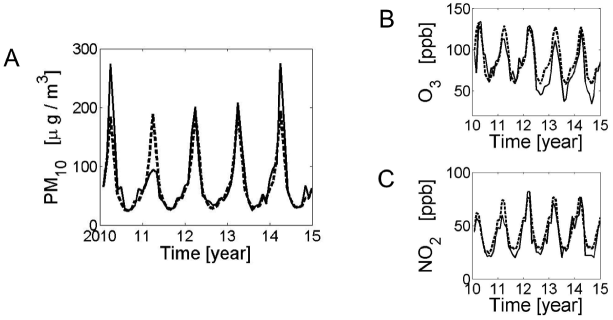
Figure 1: Extreme value pollutant concentrations (solid lines) measured in Chiangmai, North Thailand, over the five years (i.e., 60 months) period from January 2010 to December 2014. Panels A, B, C show PM₁₀, O₃, and NO₂, respectively. Dashed lines show model fits obtained from the linear regression model equation (6) in the deterministic case.

Data were taken from the Pollution Control Department (PCD) of Thailand [30]. Pollutant data for PM₁₀, O₃, and NO₂ in $N=60$ months from January 2010 to December 2014 were retrieved for the Provincial Hall measurement station in Chiangmai. Figure 1 shows the pollutant time series. The station measured raw PM₁₀ concentrations (in µg/m³) as averaged values for every day. From the daily raw data, the PCD determined for each month the maximum scores. By contrast, O₃ and NO₂, raw concentrations (in ppb) were measured by the station every hour. From those hourly raw data, maximum scores of the day and maximum values for the month were determined. The monthly extreme value data for PM₁₀, O₃, and NO₂ published on the PCD website [30] were retrieved and analyzed. As mentioned above, the study of extreme value data is of importance because extreme pollutant concentrations are related to increased health risks [18, 19, 20] and death rates [21, 22]. All three pollutants PM₁₀, O₃, and NO₂ showed periodic annual patterns (i.e., seasonal effects), see figure 1. PM₁₀ extreme value concentrations peaked in the month of March. Similarly, O₃ extreme value concentrations reached maximum values during February, March, and April. NO₂ extreme value concentrations were the largest in February and March.

For each pollutant trajectory $X(n)$, increment trajectories $Y_{n}(\tau)$ were derived for reference time points $n$ in the first three years (i.e., $n=1,\dots,R$ with $R=36$) such that each trajectory covered a two years period (i.e., $\tau=0,\dots,S$ with $S=23$). From the trajectories $Y_{n}$, scatter plots for each month $m$ showing $Y_{n}(\tau+1)$ versus $Y_{n}(\tau)$ were obtained. From the scatter plots, the drift functions $f$ were determined by means of the 3 different approximations defined by equations (4), (5) and (6). Figure 2 shows the drift functions $f(Y,m)$ thus obtained for PM₁₀ for the first four months of the year, January to April. The dashed lines represent diagonals. For January and February, all three approximations of $f$ were above the diagonals indicating that PM₁₀ increment concentrations increased during those months. That is, if increments were positive in January (February), then they tended to be positive and larger in magnitude in February (March). This describes the increase of the PM₁₀ pollutant concentration $X(n)$ towards the peaks in March (see figure 1A). By contrast, for March and April, the drift functions were found to be below the diagonals indicating the PM₁₀ increment concentrations decayed during those months. More precisely, if increments were positive in March (April), then they tended to be smaller (closer to zero) or negative in April (May). This corresponds to the decay of the PM₁₀ pollutant concentration $X(n)$ from March to May [see figure 1 (A) again].

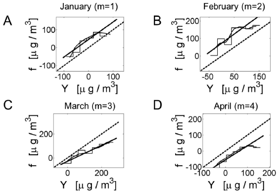
Figure 2: Drift functions $f(Y,m)$ for $Y=\rm{PM}_{10}$ extreme value concentrations determined for January, February, March, and April (panels A, B, C, and D) by means of three approximations: binning method (stair-step graphs), kernel density estimation method (solid smooth nonlinear lines), and linear regression model (solid straight lines). Dashed lines represent diagonals.

By visual inspection of figure 2, the kernel density estimation method has the advantage to account for nonlinear characteristics of $f$ in a smooth fashion. It has the disadvantage of being described by the whole data sets of $Y_{n}(\tau+1)$ and $Y_{n}(\tau)$ pairs that contribute to the relevant scatter plots. That is, each smooth function $f$ is characterized by a relatively large set of parameters given in terms of $Y_{n}(\tau+1)$ and $Y_{n}(\tau)$ pairs. The linear approximation has the advantage of being conveniently characterized by two parameters $A$ and $B$. It has the disadvantage of not capturing nonlinear effects. The drift function approximation by means of the binning method can be regarded as a compromise between the two other approximations. The stair-case like approximate drift functions obtained from the binning method account for nonlinearities. They can be described by a bin width $\Delta y$, the bin centers $y_{k,\text{c}}=(y_{k+1}+y_{k})/2$, and the function values $f_{k}$. Consequently, to describe $f$ with $K$ bins, we need $2K+1$ parameters. Therefore, the number of parameters to describe $f$ with the binning method is larger as compared to the number of parameters that characterize the linear regression model but smaller as compared to the number of $Y_{n}(\tau+1)$ and $Y_{n}(\tau)$ parameters that are needed to approximate $f$ by means of the kernel density estimation method.

The linear regression model approximation, that has the advantage of requiring the smallest number of characterizing parameters, was determined in detail for all three pollutants. That is, the parameters $A$, $B$ and $g$ were estimated as described above. Figure 3 shows the model parameters thus obtained. For all three pollutants, the intercept parameter $A$ varied across the months of the year in a characteristic pattern. For PM₁₀ and O₃ in January and February and for NO₂ in January it was positive and assumed the largest positive values. Subsequently, in March and April (PM₁₀), April and May (O₃ and NO₂), parameter $A$ was negative and assumed the largest-in-the-amount negative values. These patterns, as discussed above in the context of PM₁₀ and figure 2, describe the mechanism that leads to the peaks in the original trajectories $X(n)$ around February, March, and April, see figure 1. For the remaining months from May to December, the intercept parameters $A$ were overall relatively small (i.e., close to zero). PM₁₀ and O₃ showed exceptions from this rule in September, where the parameter values $A$ were positive and assumed 20% (PM₁₀) and 45% (O₃) of their respective maximal positive $A$ parameters. For all three pollutants, the slope parameter $B$ was found to be relatively close to unity. For PM₁₀ and NO₂, the noise amplitude $g$ showed clear seasonal peaks around January, February, and March (PM₁₀) and March and April (NO₂).

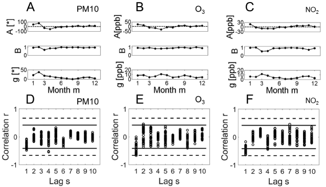
Figure 3: Model parameters $A$, $B$, and $g$ as functions of month $m$ of the linear regression model equation (6) for the pollutants PM₁₀ (panel A), O₃ (panel B), and NO₂ (panel C). Here, $*$ in panel A means µg/m³. Panels D, E, F: Lag-$s$ autocorrelation coefficients of residuals for PM₁₀ (panel D), O₃ (panel E), and NO₂ (panel F) with thresholds for statistical significance (see text).

In order to validate the model, we tested the residuals $\epsilon$ occurring in equation (6). We determined the first ten lag-$s$ autocorrelation coefficients of the residuals for each trajectory $Y_{n}(\tau)$. The coefficients are shown in figure 3 (panels D, E, F) together with single-time-series thresholds [31] (solid lines) for statistically significant and Bonferroni adjusted [32] multiple-tests thresholds (dashed lines). We found that some of the correlation coefficients (in particular, lag-1 correlation coefficients of O₃ and NO₂) violated the single-time-series criterion for being not statistically significant. However, all correlation coefficients were found to be within the boundaries of the multiple-tests thresholds. Residuals of trajectories $Y_{n}(\tau)$ were also tested for violation of normality using the Anderson-Darling normality test. For all PM₁₀ and NO₂ trajectories $Y_{n}(\tau)$, the residuals did not violate the normality assumption. For O₃, the normality assumption was violated in 4 out of $R=36$ trajectories $Y_{n}$. Overall, the correlation and normality tests supported the model assumptions.

We showed how to identify stochastic dynamical models for the evolution of air pollutants on the basis of single, historical trajectories of pollutant concentrations. To this end, we followed the earlier work on financial data and considered pollutant increments rather than the raw pollutant data. In addition, three different representation methods of the drift functions of the dynamical models were used. In doing so, we derived three main results: First, we found that all three representation methods were consistent with each other, see figure 2. Second, we were able to show that experimentally observed annual air pollutant peaks were caused by drift functions of physical-chemical air pollutant systems that change qualitatively from the pre-peak months (e.g., January and February) to the post-peak months (e.g., March and April), see figure 2 again. These qualitative changes in the drift functions are assumed to reflect periodic changes in the physical-chemical laws determining the evolution of the PM₁₀, O₃, and NO₂ pollutant concentrations. Third, it was found that the linear approximation representation method of drift functions (which is the most parsimony method) is sufficient to reproduce the emergence of the yearly pollutant peaks, see figure 1.

Ukrainian 0 Здiйснення дрейф-дифузiйного аналiзу через дослiдження турбулентних потокiв та динамiки частинок речовини смогу i забруднювачiв повiтря T. Варапонгпiсан${}^{\textsf{\footnotesize{\mbox{?}}}}$, Л. Iнгрiсвванг${}^{\textsf{\footnotesize{\mbox{?}}}}$, Т.Д. Френк${}^{\textsf{\footnotesize{\mbox{?},\penalty 1000\mbox{?}}}}$

             
${}^{\textsf{\footnotesize 1}}$ Факультет природничих наук, вiддiлення фiзики, унiверситет Касертсарт, Бангкок 10900, Таїланд ${}^{\textsf{\footnotesize 2}}$ CESPA, вiддiлення психологiї, Коннектикутський унiверситет, CT 06269, США ${}^{\textsf{\footnotesize 3}}$ Вiддiлення фiзики, Коннектикутський унiверситет, CT 06269, США

References

- [1] Friedrich R., Peinke J., Phys. Rev. Lett., 1997, 78, 863, doi:10.1103/PhysRevLett.78.863.
-
[2]
Khomenko A.V., Lyashenko I.A., Borisyuk V.N., Fluctuation Noise Lett.,
2010, 9, 19,
doi:10.1142/S0219477510000046. - [3] Friedrich R., Peinke J., Physica D, 1997, 102, 147, doi:10.1016/S0167-2789(96)00235-7.
- [4] Naert A., Friedrich R., Peinke J., Phys. Rev. E, 1997, 56, 6719, doi:10.1103/PhysRevE.56.6719.
- [5] Tutkun M., Mydlarski L., New J. Phys., 2004, 6, 49, doi:10.1088/1367-2630/6/1/049.
- [6] Kuwahara J., Miyata H., Konno H., AIP Conf. Proc., 2017, 1872, 020013, doi:10.1063/1.4996670.
- [7] Friedrich R., Peinke J., Sahimi M., Tabar M.R.R., Phys. Rep., 2011, 506, 87, doi:10.1016/j.physrep.2011.05.003.
- [8] Davies B.L., Kurz M.J., Res. Dev. Disabilities, 2013, 34, 3648, doi:10.1016/j.ridd.2013.08.012.
-
[9]
Kurz M.J., Arpin D.J., Davies B.L., Harbourne R., Ann. Biomed. Eng., 2013, 41, 1703,
doi:10.1007/s10439-013-0821-7. - [10] Van Mourik A.M., Daffertshofer A., Beek P.J., Phys. Lett. A, 2006, 351, 13, doi:10.1016/j.physleta.2005.10.066.
- [11] Frank T.D., Friedrich R., Beek P.J., Phys. Rev. E, 2006, 74, 051905, doi:10.1103/PhysRevE.74.051905.
- [12] Gottschall J., Peinke J., Lippens V., Nagel V., Phys. Lett. A, 2009, 373, 811, doi:10.1016/j.physleta.2008.12.026.
- [13] Frank T.D., Sondermann M., Ackemann T., Friedrich R., Nonlinear Phenom. Complex Syst., 2005, 8, 193.
- [14] Chiangga S., Frank T.D., Nonlinear Phenom. Complex Syst., 2010, 13, 32.
- [15] Gradišek J., Siegert S., Friedrich R., Grabec I., Phys. Rev. E, 2000, 62, 3146, doi:10.1103/PhysRevE.62.3146.
- [16] Lind P.G., Wächter M., Peinke J., J. Phys. Conf. Ser., 2014, 524, 012179, doi:10.1088/1742-6596/524/1/012179.
- [17] Noiray N., J. Eng. Gas Turbines Power, 2016, 139, 041503, doi:10.1115/1.4034601.
- [18] Li D., Wang J., Zhang Z., Shen P., Zheng P., Jin M., Lu H., Lin H., Chen K., Environ. Sci. Pollut. Res., 2018, 25, 16135, doi:10.1007/s11356-018-1759-y.
-
[19]
Maji K.J., Dikshit A.K., Deshpande A., Environ. Sci. Pollut. Res., 2017, 24, 4709,
doi:10.1007/s11356-016-8164-1. -
[20]
Pope C.A. III, Dockery D.W., J. Air Waste Manage. Assoc., 2006, 56, 709,
doi:10.1080/10473289.2006.10464485. -
[21]
Giri D., Murthy V.K., Adhikary P.R., Khanal S.N., Int. J. Environ. Sci. Technol.,
2007, 4, 183,
doi:10.1007/BF03326272. - [22] Montero Lorenzo J.M., Sánchez-Ollero J.L., Fernandez-Aviles G., Int. J. Environ. Res., 2011, 5, 23, doi:10.22059/ijer.2010.287.
- [23] Vichit-Vadakan N., Vajanapoom N., Environ. Health Perspect., 2011, 119, 197, doi:10.1289/ehp.1103728.
- [24] Friedrich R., Peinke J., Renner Ch., Phys. Rev. Lett., 2000, 84, 5224, doi:10.1103/PhysRevLett.84.5224.
- [25] Risken H., The Fokker-Planck Equation: Methods of Solution and Applications, Springer, Berlin, 1989.
- [26] Frank T.D., Nonlinear Fokker-Planck Equations: Fundamentals and Applications, Springer, Berlin, 2005.
- [27] Stanton R., J. Finance, 1997, 52, 1973, doi:10.1111/j.1540-6261.1997.tb02748.x.
- [28] Silverman B.W., Density Estimation for Statistics and Data Analysis, Chapman and Hall, London, 1986.
- [29] Frank T.D., Physica A, 2008, 387, 773, doi:10.1016/j.physa.2007.10.027.
- [30] PCD (Pollution Control Department, Thailand), Ministry of Natural Resources and Environment, Thailand, accessed 2018, http://air4thai.pcd.go.th/webV2/download.php (in Thai).
- [31] Diggle P.J., Time Series: a Biostatistical Introduction, The Clarendon Press, Oxford, 1990.
- [32] Keppel G., Wickens T.D., Design and Analysis, Pearson Prentice Hall, New Jersey, 2004.
Ukrainian \adddialect\l@ukrainian0 \l@ukrainian Здiйснення дрейф-дифузiйного аналiзу через дослiдження турбулентних потокiв та динамiки частинок речовини смогу i забруднювачiв повiтря T. Варапонгпiсан, Л. Iнгрiсвванг, Т.Д. Френк