A Gradient Sampling method based on Ideal direction for solving nonsmooth nonconvex optimization problems

Abstract

In this paper, a modification to the Gradient Sampling (GS) method for minimizing nonsmooth nonconvex functions is presented. One drawback in GS method is the need of solving a Quadratic optimization Problem (QP) at each iteration, which is time-consuming especially for large scale objectives. To resolve this difficulty, we propose a new descent direction, namely Ideal direction, for which there is no need to consider any quadratic or linear optimization subproblem. It is shown that, this direction satisfies Armijo step size condition and can be used to make a substantial reduction in the objective function. Furthermore, we prove that using Ideal directions preserves the global convergence of the GS method. Moreover, under some moderate assumptions, we present an upper bound for the number of serious iterations. Using this upper bound, we develop a different strategy to study the convergence of the method. We also demonstrate the efficiency of the proposed method using small, medium and large scale problems in our numerical experiments.

1 Introduction

In this paper, we consider the following unconstrained minimization problem

$$\min f({\mathbf{x}})\quad\text{s.t.}\quad{\mathbf{x}}\in\mathbb{R}^{n}$$ (1)

where $f:\mathbb{R}^{n}\to\mathbb{R}$ is locally Lipschitz and continuously differentiable on an open set $D$ with full measure in $\mathbb{R}^{n}$. These types of problems arise in many applications, such as optimal control, image processing, data analysis, economics, chemistry and biology (Makela_book ; image ; Poly-approx ; bio-ch2 ; data-mining ). Therefore, it is worthwhile to develop efficient algorithms for solving such problems. During the last three decades, a lot of effort has gone into nonsmooth optimization. In particular, Clarke developed the concept of subgradient in Clarke1990 and soon after, it became the cornerstone of designing and developing many algorithms in nonsmooth optimization (see Makela_book ; kiwielbook ; shorbook ; lemarchal-book1 ; lemarchal-book2 ; v-metric1 ; v-metric2 ).

When it comes to designing numerical methods for minimizing nonsmooth functions, there are serious challenges we need to deal with. The main difficulty is that, nonsmooth functions are generally not differentiable at stationary points. Finding a descent direction is not an easy task as well. In smooth case, any vector has an obtuse angle with the gradient is a descent direction. In particular, the vector $-\nabla f({\mathbf{x}})$ defines the steepest descent direction. In contrast, in the nonsmooth case a vector that is opposite to an arbitrary subgradient need not be a direction of descent and hence designing descent algorithms is much more complicated. These difficulties make most of classic methods in smooth optimization unsuitable for solving nonsmooth optimization problems. For instance, it is well known that when the ordinary steepest descent method is applied to a nonsmooth function, it generally fails to make a substantial reduction in objective function as it approaches a nonsmooth region.

There are various methods for locating minimizers of nonsmooth functions. The subgradient method, originally proposed by N. Shor shorbook , is one of the simplest methods for minimizing nonsmooth functions. Due to its simple structure, it is a popular method, although it suffers from some serious limitations such as slow convergence, lack of practical termination criterion and lack of descent. However, it is well known that some of its modifications are able to overcome these difficulties (see bagirov2012 ; m-amiri ; Nesterov ; bagirov2010 ). As another class of nonsmooth methods, we can refer to Bundle methods as one of the most efficient methods in nonsmooth optimization lemarchal-book1 ; lemarchal-book2 ; kiwielbook . The key idea of bundle methods is to keep memory of computed subgradients at previous iterations to construct a piecewise linear model for objective function. These methods require a great deal of storage, therefore some of its modifications presented in Haarala ; Luksan are more efficient for solving large scale nonsmooth problems. In class of subgradient and bundle methods, at each iteration, the user needs to supply at least one subgradient. However, in many cases computing only one subgradient is not an easy task. In such situations, Gradient Sampling (GS) methods are more efficient, because they obtain a search direction without explicit computation of subgradients.

The gradient sampling algorithm, originally developed by Burke, Lewis and Overton Burke2005 , is a descent method for solving problem (1). The method is robust and can be applied to a broad range of nonsmooth functions. A comprehensive discussion of the GS algorithm along with its last modifications can be found in the recent paper GS-full . The convergence analysis and theoretical results of the GS algorithm were first developed in Burke2005 . Soon after, these results were strengthen by the work of Kiwiel in Kiwiel2007 . In particular, under subtle modifications, Kiwiel derived a lower bound for step sizes and suggested a limited Armijo line search in which the number of backtracking steps can be managed through our choice of initial step size. Another version of the GS method in which the Clarke $\varepsilon$-subdifferential is approximated by sampling estimates of mollifier gradients presented by Kiwiel in Kiwiel2010 . In the work of Curtis and Que Curtis2013 , two novel strategies were introduced to improve the efficiency of the GS method. The first strategy is to combine the idea of sampling gradients and LBFGS update (see nocedal ) to approximate Hessian matrix. The second one uses the idea of sampling gradients to provide a model that overestimates the objective function. In both techniques, the dual of the quadratic subproblem is considered for warm-starting the QP solver. In the work of Curtis and Overton Curtis2012 , the ideas of gradient sampling and Sequential Quadratic Programming (SQP) are combined for solving nonsmooth constrained optimization problems. In addition, the local convergence rate of the GS algorithm for the class of finite-max functions is studied in C-Rate . These continued developments clearly indicate that, the GS technique has been a reach area of research.

However, the GS method suffers from two practical limitations. First, in order to obtain an approximation of $\varepsilon$-steepest descent direction, the GS method requires to compute gradient information at $m\geq n+1$ randomly generated points during each iteration. It is noted that, for large scale objectives, this may not be tractable at a moderate cost. To alleviate this difficulty, In Curtis2013 , Curtis and Que proposed an adaptive strategy in which the convergence of the method is guaranteed only through $\mathcal{O}(1)$ gradient evaluations at each iteration. The second limitation is to solve the corresponding QP. As the number of variables increases, the size of this QP increases significantly which makes the method unsuitable for large scale objectives. Furthermore, when we are far away from a nonsmooth region, since the information collected by sampling gradients are very close together, solving the quadratic subproblem is not reasonable. Nevertheless, since checking differentiability of $f$ is not an easy task, the GS method and its modifications do not care about this fact. In this work, we address the second difficulty by introducing a new search direction.

In this paper, based on gradient sampling technique, we propose a new search direction, namely Ideal direction, for which there is no need to consider any kind of quadratic or linear subproblems. Furthermore, we show that this direction satisfies Armijo step size condition and provides a necessary optimality condition in the sense that it vanishes at optimality. The original GS method is modified using Ideal directions. By means of this new search direction, not only is there no need to solve the quadratic subproblem in smooth regions, but also we can reduce the number of quadratic subproblems once the method starts tracking a nonsmooth curve which leads to a stationary point. Moreover, we provide a comprehensive discussion for the convergence analysis of the method. We follow closely the work of Kiwiel in Kiwiel2007 to analyze the convergence of the proposed method. Of course, there are some differences due to using Ideal directions. In addition, thanks to the limited Armijo line search proposed in Kiwiel2007 , we present an upper bound for the number of serious iterations generated in our method. Using this upper bound, a different strategy to study the global convergence behavior of the proposed method is developed assuming that the objective function is bounded below.

This paper is organized as follows. Section 2 provides some mathematical preliminaries used in this paper. A brief review over the GS method is presented in Sect. 3. In Sect. 4, we introduce Ideal direction and its main properties are examined. The proposed method and its convergence analysis are given in Sect. 5. Numerical results are reported in Sect. 6 and Sect. 7 concludes the paper.

2 Preliminaries

We use the following notations in this paper. As usual, $\mathbb{R}^{n}$ is the $n$-dimensional Euclidean space and its inner product is denoted by $\langle{\mathbf{x}},\mathbf{y}\rangle:=\sum_{k=1}^{n}x_{i}y_{i}$ that induces the associated Euclidean norm $\lVert{\mathbf{x}}\rVert$:=$\langle{\mathbf{x}},{\mathbf{x}}\rangle^{1/2}$. $B({\mathbf{x}},\varepsilon):=\{\mathbf{y}\in\mathbb{R}^{n}:\lVert\mathbf{y}-{\mathbf{x}}\rVert\leq\varepsilon\}$ is the closed ball centered at ${\mathbf{x}}$ with radius $\varepsilon$. Furthermore $B_{\varepsilon}:=B(\mathbf{0},\varepsilon)$.

A function $f:\mathbb{R}^{n}\to\mathbb{R}$ is called locally Lipschitz Bagirov2014 , if for every ${\mathbf{x}}\in\mathbb{R}^{n}$ there exist positive constants $K_{\mathbf{x}}$ and $\varepsilon_{\mathbf{x}}$ such that

$$|f(\mathbf{z})-f(\mathbf{y})|\leq K_{\mathbf{x}}\lVert\mathbf{z}-\mathbf{y}\rVert\,,\quad\text{for \,all}\,\,\mathbf{z},\mathbf{y}\in B({\mathbf{x}},\varepsilon_{\mathbf{x}}).$$

Let

$$\Omega_{f}:=\{{\mathbf{x}}\in\mathbb{R}^{n}\,:\,f\,\,\text{is not differentiable at }{\mathbf{x}}\},$$

be the subset of $\mathbb{R}^{n}$ where the function $f$ is not differentiable. By Rademacher’s theorem Evans2015 , every locally Lipschitz function is differentiable almost everywhere. Therefore, the Clarke subdifferential of a locally Lipschitz function $f$ at a point ${\mathbf{x}}\in\mathbb{R}^{n}$ can be given by Clarke1990

$$\partial f({\mathbf{x}}):=\texttt{co}\{{\boldsymbol{\xi}}\in\mathbb{R}^{n}:\exists\,\{{\mathbf{x}}_{k}\}\subset\mathbb{R}^{n}\setminus\Omega_{f}\,\,\,\,\text{s.t.}\,\,\,\,{\mathbf{x}}_{k}\to{\mathbf{x}}\,\,\,{\rm and}\,\,\,\,\nabla f({\mathbf{x}}_{k})\to{\boldsymbol{\xi}}\},$$

in which co stands for the convex hull. It is shown in Bagirov2014 that the set valued map $\partial f:\mathbb{R}^{n}\rightrightarrows\mathbb{R}^{n}$ is outer semicontinuous and the set $\partial f({\mathbf{x}})$ is a convex compact subset of $\mathbb{R}^{n}.$ The Clarke $\varepsilon$-subdifferential, which is the generalization of ordinary subdifferential, is defined by Bagirov2014

$$\partial_{\varepsilon}f({\mathbf{x}}):=\texttt{cl\,co}\,\partial f({\mathbf{x}}+B_{\varepsilon}).$$

Clearly, the set valued map $\partial_{\varepsilon}f:\mathbb{R}^{n}\rightrightarrows\mathbb{R}$ has a closed graph and hence it is outer semicontinuous Rockafellar2004 .

Suppose that $f:\mathbb{R}^{n}\to\mathbb{R}$ is locally Lipschitz and continuously differentiable on an open set $D$ with full measure in $\mathbb{R}^{n}$. The following representation of the Clarke subdifferential is the key idea of approximating subdifferential set by sampling gradients Clarke1990

$$\partial f({\mathbf{x}})=\bigcap_{\varepsilon>0}G_{\varepsilon}({\mathbf{x}}),$$

such that

$$G_{\varepsilon}({\mathbf{x}}):=\texttt{cl\,co}\{\nabla f(({\mathbf{x}}+B_{\varepsilon})\cap D)\},$$

where cl denotes the closure of a set. Let ${\mathbf{x}}\in\mathbb{R}^{n}$ be a differentiable point, $\varepsilon>0$, $m\in\mathbb{N}$ and $\mathbf{u}_{1},...,\mathbf{u}_{m}$ be sampled uniformly and independently from $B_{1}$. If $\mathbf{s}_{0}:={\mathbf{x}}$ and $\mathbf{s}_{i}:={\mathbf{x}}+\varepsilon\mathbf{u}_{i}$ is a differentiable point for $i=1,\ldots,m$, then the gradient bundle $G^{m}_{\varepsilon}(\mathbf{x})$ is defined as Burke2005 ; Kiwiel2007

$$G^{m}_{\varepsilon}({\mathbf{x}}):=\texttt{co}\{\nabla f(\mathbf{s}_{0}),\nabla f(\mathbf{s}_{1}),\ldots,\nabla f(\mathbf{s}_{m})\},$$ (2)

in which $\epsilon>0$ and $m\in\mathbb{N}$ are called sampling radius and sample size respectively. For a locally Lipschitz function $f$, it is easy to see that

$$G^{m}_{\varepsilon}({\mathbf{x}})\subset G_{\varepsilon}({\mathbf{x}})\subset\partial_{\varepsilon}f({\mathbf{x}}),$$

and for $0<\varepsilon_{1}<\varepsilon_{2}$, we have $\partial_{\varepsilon_{1}}f({\mathbf{x}})\subset G_{\varepsilon_{2}}({\mathbf{x}})$. Furthermore, it is proved in GS-full that for every ${\mathbf{x}}\in\mathbb{R}^{n}$ and $\varepsilon>0$

$$\partial f({\mathbf{x}})\subset G_{\varepsilon}({\mathbf{x}}).$$

The following definition provides a useful point of view to study the concept of gradient sampling.

Definition 1

For a locally Lipschitz function $f:\mathbb{R}^{n}\to\mathbb{R}$ and optimality tolerance $\nu>0$, a point $\mathbf{x}\in\mathbb{R}^{n}$ is called a $(\nu,G^{m}_{\epsilon}(\mathbf{x}))$-stationary point if

$$\min\{\lVert\mathbf{g}\rVert:\mathbf{g}\in G^{m}_{\epsilon}(\mathbf{x})\}\leq\nu.$$

We recall that, if ${\mathbf{x}}\in\mathbb{R}^{n}$ is a local minimum of a locally Lipschitz function $f$, then it is necessary that Bagirov2014

$$\mathbf{0}\in\partial f({\mathbf{x}}).$$

The point ${\mathbf{x}}\in\mathbb{R}^{n}$ satisfying the above condition is called Clarke stationary point. Furthermore, a point ${\mathbf{x}}\in\mathbb{R}^{n}$ is called Clarke $\varepsilon$-stationary point if

$$\mathbf{0}\in\partial_{\varepsilon}f({\mathbf{x}}).$$

3 Background on GS method

The Gradient Sampling (GS) method Burke2005 is a descent method for solving problem (1). At each iteration of the method, the steepest descent direction is approximated and utilized to make a substantial reduction in $f$. In this method, the concepts of steepest descent direction and choosing step size are crucial. In this respect, these concepts are briefly reviewed .

3.1 The steepest descent direction

We recall that, a direction ${\mathbf{d}}\in\mathbb{R}^{n}$ is called a direction of descent for $f:\mathbb{R}^{n}\to\mathbb{R}$ at ${\mathbf{x}}\in\mathbb{R}^{n}$, if there is $z_{0}>0$ such that

$$f({\mathbf{x}}+t\mathbf{d})-f({\mathbf{x}})<0,\qquad\text{for \,all}\,\,t\in(0,z_{0}].$$ (3)

In the descent methods, choosing a step size $t$ satisfying the above inequality does not guarantee the convergence of the method. In this regard, some sufficient decrease conditions are introduced kiwielbook . Among them, an Armijo step size condition, which is commonly used in GS methods, is considered to state the following definition.

Definition 2

Let $\mathbf{g}\neq\mathbf{0}$, we say that $\mathbf{g}$ induces an Armijo Descent Direction (ADD) $\mathbf{d}:=-\lVert\mathbf{g}\rVert^{-1}\mathbf{g}$ for $f$ at point $\mathbf{x}$, if for each $c\in(0,1)$ there is $z_{0}>0$ such that

$$f({\mathbf{x}}+t\mathbf{d})-f({\mathbf{x}})<-ct\lVert\mathbf{g}\rVert,\qquad{\rm{for\,\,all}}\,\,t\in(0,z_{0}].$$

The above condition is called sufficient decrease condition.

If $f$ is smooth at a point ${\mathbf{x}}\in\mathbb{R}^{n}$, then every descent direction at this point is an ADD toonocedal . However, this is not the case when $f$ is not smooth at ${\mathbf{x}}$. Therefore, in order to design a descent method for minimizing a nonsmooth function, providing an ADD is essential to ensure the convergence of the method.

To define the concept of steepest descent direction for a locally Lipschitz function more precisely, we need to generalize the classical directional derivative. For a smooth or convex function $f:\mathbb{R}^{n}\to\mathbb{R}$, the classical directional derivative is defined as

$$f^{\prime}({\mathbf{x}};{\mathbf{d}}):=\lim_{t\downarrow 0}t^{-1}[f({\mathbf{x}}+t\mathbf{d})-f({\mathbf{x}})],$$ (4)

and the steepest descent direction at the point ${\mathbf{x}}\in\mathbb{R}^{n}$ is obtained by solving the problem

$$\min_{\lVert{\mathbf{d}}\rVert\leq 1}f^{\prime}({\mathbf{x}};{\mathbf{d}}).$$

However, the quantity (4) does not always exist for locally Lipschitz functions. In this regard, for locally Lipschitz functions, the Clarke generalized directional derivative is defined as Bagirov2014

$$f^{\circ}({\mathbf{x}};{\mathbf{d}}):=\limsup_{\begin{subarray}{c}\mathbf{y}\to{\mathbf{x}}\\ t\downarrow 0\end{subarray}}\,t^{-1}[f(\mathbf{y}+t\mathbf{d})-f(\mathbf{y})].$$

Moreover, it is shown that this directional derivative can be expressed as Bagirov2014

$$f^{\circ}({\mathbf{x}};{\mathbf{d}})=\max_{{\boldsymbol{\xi}}\in\partial f({\mathbf{x}})}\langle{\boldsymbol{\xi}},{\mathbf{d}}\rangle,$$

and naturally, the steepest descent direction of a locally Lipschitz function $f$ at the point ${\mathbf{x}}\in\mathbb{R}^{n}$ can be obtained by solving the following $\min$-$\max$ problem

$$\min_{\lVert{\mathbf{d}}\rVert\leq 1}\,\max_{{\boldsymbol{\xi}}\in\partial f({\mathbf{x}})}\langle{\boldsymbol{\xi}},{\mathbf{d}}\rangle.$$ (5)

Using von Neumann minimax theorem convex_book , the above problem is equivalent to the following problem

$$\min_{{\boldsymbol{\xi}}\in\partial f({\mathbf{x}})}\,\lVert{\boldsymbol{\xi}}\rVert,$$ (6)

in the sense that, if ${\boldsymbol{\xi}}^{*}\neq 0$ is the solution of the problem (6), then ${\mathbf{d}}^{*}=-\lVert{\boldsymbol{\xi}}^{*}\rVert^{-1}{\boldsymbol{\xi}}^{*}$ solves the problem (5). As a result, to obtain the steepest descent direction it is sufficient to find the member of subdifferential set with minimum norm.

In an iterative descent method for minimizing a nonsmooth function, after some iterations, the method rapidly approaches a nonsmooth curve leading to a stationary point. Therefore, it is likely that, the method generates a sequence of smooth points that are close to the nonsmooth curve. In such cases, since the Clarke subdifferential is a singleton set, the steepest descent direction is not an efficient direction, while the Clarke $\varepsilon$-subdifferential is able to collect some information of the nonsmooth curve and hence the so-called $\varepsilon$-steepest descent direction is a more suitable search direction.

In a similar fashion, the $\varepsilon$-steepest descent direction at the point ${\mathbf{x}}\in\mathbb{R}^{n}$ can be obtained from the solution of the following problem

$$\min_{{\boldsymbol{\xi}}\in\partial_{\varepsilon}f({\mathbf{x}})}\,\lVert{\boldsymbol{\xi}}\rVert.$$ (7)

However, since solving the problem (7) requires the knowledge of the whole subdifferential on $B({\mathbf{x}},\varepsilon)$, computing the $\varepsilon$-steepest descent direction is cumbersome. To overcome this drawback, since $G^{m}_{\varepsilon}({\mathbf{x}})$ is a proper inner approximation of $\partial_{\varepsilon}f({\mathbf{x}})$, the $\varepsilon$-steepest descent direction is approximated through replacing $\partial_{\varepsilon}f({\mathbf{x}})$ by $G^{m}_{\varepsilon}({\mathbf{x}})$ in the problem (7) and the approximate $\varepsilon$-steepest descent direction can be obtained from the following problem

$$\min_{{\mathbf{g}}\in G^{m}_{\varepsilon}({\mathbf{x}})}\,\lVert{\mathbf{g}}\rVert.$$ (8)

Indeed, the problem (8) is a Quadratic Problem (QP). To state this fact, by Carathéodory’s theorem Bazaraa2006 , this problem can be written in the following quadratic programing form

$$\min_{\boldsymbol{\lambda}}\,\frac{1}{2}\lVert G\boldsymbol{\lambda}\rVert^{2}$$ (9)

$$\text{ s.t.}\quad\sum_{i=0}^{m}\lambda_{i}=1,\quad\lambda_{i}\geq 0,\quad\,i=0,\ldots,m,$$

where $G:=[\nabla f(\mathbf{s}_{0})\,\,\nabla f(\mathbf{s}_{1})\ldots\nabla f(\mathbf{s}_{m})]\in\mathbb{R}^{n\times(m+1)}$ and $\boldsymbol{\lambda}^{t}:=(\lambda_{0},\lambda_{1},\ldots,\lambda_{m})\in\mathbb{R}^{m+1}$. We summarize the concept of approximate $\varepsilon$-steepest descent direction in the following definition.

Definition 3

Suppose that $\mathbf{0}\notin G^{m}_{\varepsilon}({\mathbf{x}})$ and $\boldsymbol{\lambda}^{*}$ is the solution of the problem (9). Let ${\mathbf{g}}^{\text{\rm\tiny{s}}}_{\varepsilon}:=G\boldsymbol{\lambda}^{*}$. Then the direction $\mathbf{d}^{\text{\rm\tiny{s}}}_{\varepsilon}:=-\lVert{\mathbf{g}}^{\text{\rm\tiny{s}}}_{\varepsilon}\rVert^{-1}{\mathbf{g}}^{\text{\rm\tiny{s}}}_{\varepsilon}$ is called (normalized) approximate $\varepsilon$-steepest descent direction.

It is noted that, the approximate $\varepsilon$-steepest descent direction is an ADD Burke2005 . In other words, for the direction ${\mathbf{d}}^{\text{\rm\tiny{s}}}_{\varepsilon}$ and each $c\in(0,1)$, there exists $z_{0}>0$ such that

$$f({\mathbf{x}}+t{\mathbf{d}}^{\text{\rm\tiny{s}}}_{\varepsilon})-f({\mathbf{x}})<-tc\lVert{\mathbf{g}}^{\text{\rm\tiny{s}}}_{\varepsilon}\rVert,\qquad\text{for \,all}\,\,t\in(0,z_{0}].$$ (10)

3.2 Choosing stepsize and backtracking line search

Loosely speaking, the GS method is a descent method in which at each iteration the approximate $\varepsilon$-steepest descent direction is considered as the search direction. Therefore, the QP (9) is solved per iteration and then a backtracking line search is applied to find the step size $t$ as stated in Algorithm 1.

1

2

inputs : ${\mathbf{x}}\in\mathbb{R}^{n}$, the directions ${\mathbf{d}},\mathbf{g}\in\mathbb{R}^{n}$, parameters $\gamma,c\in(0,1)$.

output : Step size $t$.

requied : ${\mathbf{d}}=-\lVert\mathbf{g}\rVert^{-1}\mathbf{g}$ is an ADD for $f$ at ${\mathbf{x}}$.

3

4 Function BALS($\mathbf{x}$, $\mathbf{g}$, $\mathbf{d}$, $\gamma$, $c$):

5       $t:=1$;

6       while $f({\mathbf{x}}+t{\mathbf{d}})-f({\mathbf{x}})\geq-ct\lVert{\mathbf{g}}\rVert$ do

7             $t:=\gamma t$;

8            

9       end while

10      return $t$;

11      

12

End Function

Algorithm 1 Backtracking Armijo Line Search (BALS)

In Algorithm 1, the following termination condition

$$f({\mathbf{x}}+t\mathbf{d})-f({\mathbf{x}})<-ct\lVert\mathbf{g}\rVert,$$ (11)

is called sufficient decrease condition. It is stressed that, for an ADD this algorithm finds a step size $t>0$ after finitely iterations.

3.3 GS method

The main aim of the GS method is to produce a Clarke stationary point through a sequence of $(\nu_{k},G^{m}_{\varepsilon_{k}}(\mathbf{x}_{k}))$-stationary points where $\{\nu_{k}\}$ and $\{\varepsilon_{k}\}$ are decreasing sequences that tend to zero. To provide more details, at each iteration, the set of sampled points $\{\mathbf{s}_{k1},\ldots,\mathbf{s}_{km}\}\cup\{\mathbf{s}_{k0}\}$ is generated uniformly and independently from $B({\mathbf{x}}_{k},\varepsilon_{k})$ and then the gradient information of the objective function is computed at these points. Next, ${\mathbf{g}}^{\text{\rm\tiny{s}}}_{\varepsilon_{k}}$ is obtained by solving the QP (9) and then the optimality condition

$$\lVert{\mathbf{g}}^{\text{\rm\tiny{s}}}_{\varepsilon_{k}}\rVert\leq\nu_{k},$$ (12)

is checked. If condition (12) does not hold, ${\mathbf{x}}_{k}$ is not a $(\nu_{k},G^{m}_{\varepsilon_{k}}(\mathbf{x}_{k}))$-stationary point. In this case, the sampling radius and the optimality tolerance remain unchanged, the approximate $\varepsilon$-steepest descent direction $\mathbf{d}^{\text{\rm\tiny{s}}}_{\varepsilon_{k}}=-\lVert\mathbf{g}^{\text{\rm\tiny{s}}}_{\varepsilon_{k}}\rVert^{-1}\mathbf{g}^{\text{\rm\tiny{s}}}_{\varepsilon_{k}}$ is considered as the search direction, the the step size $t_{k}$ is computed by the Algorithm 1 using inputs $(\mathbf{x}_{k},\mathbf{g}^{\text{\rm\tiny{s}}}_{\varepsilon_{k}},\mathbf{d}^{\text{\rm\tiny{s}}}_{\varepsilon_{k}},\gamma,c)$ and finally the current point ${\mathbf{x}}_{k}$ is updated by ${\mathbf{x}}_{k+1}:={\mathbf{x}}_{k}+t_{k}\mathbf{d}^{\text{\rm\tiny{s}}}_{\varepsilon_{k}}$. To ensure the convergence of the GS method, the point $\mathbf{x}_{k+1}$ must be a differentiable point. Consequently, if the objective function is not differentiable at ${\mathbf{x}}_{k+1}$, a differentiable point, say $\mathbf{\hat{x}}$, having the following properties Kiwiel2007

$$f(\mathbf{\hat{x}})-f({\mathbf{x}}_{k})<-ct_{k}\lVert\mathbf{g}^{\text{\rm\tiny{s}}}_{\varepsilon_{k}}\rVert,$$ (13)

$$\lVert{\mathbf{x}}_{k}+t_{k}\mathbf{d}^{\text{\rm\tiny{s}}}_{\varepsilon_{k}}-\mathbf{\hat{x}}\rVert\leq\min\{t_{k},\varepsilon_{k}\},$$ (14)

is selected as a perturbation of ${\mathbf{x}}_{k+1}$ and ${\mathbf{x}}_{k+1}$ is updated by $\mathbf{\hat{x}}$. A procedure to find such a perturbation can be found in Kiwiel2007 . We shall see later the motivation of the inequalities (13) and (14) in Sect. 5. On the other hand, if condition (12) holds, ${\mathbf{x}}_{k}$ is a $(\nu_{k},G^{m}_{\varepsilon_{k}}(\mathbf{x}_{k}))$-stationary point. In this case, the sampling radius and the optimality tolerance are decreased by their corresponding reduction factors, the gradient bundle $G^{m}_{\varepsilon_{k}}(\mathbf{x}_{k})$ is resampled and the process is repeated.

The GS method is robust and can be used for solving a broad range of nonsmooth problems, but it still suffers from some limitations. Here, we highlight some of these drawbacks that are addressed in this paper.

• For the large scale objectives the QP (9) is a time-consuming subproblem that is solved at each iteration. This fact makes the GS method unsuitable for large scale nonsmooth problems GS-full .

• When the objective function $f$ is smooth on $B({\mathbf{x}}_{k},\varepsilon_{k})$ (this is the case in early iterations of the method) the information we collect by sampling gradients are close together and there is not any significant difference between $-\lVert{\mathbf{g}}^{\text{\rm\tiny{s}}}_{\varepsilon_{k}}\rVert^{-1}{\mathbf{g}}^{\text{\rm\tiny{s}}}_{\varepsilon_{k}}$ and $-\lVert\nabla f({\mathbf{x}}_{k})\rVert^{-1}\nabla f({\mathbf{x}}_{k})$ as a search direction. In such cases, solving the QP (9) is not reasonable.

To resolve the above limitations, we introduce an alternative direction, namely Ideal direction, that can be computed fast in comparison to solving the QP (9). Moreover, this direction may help us to check the optimality condition (12) without solving the QP (9).

4 Ideal direction

To overcome the aforementioned difficulties, we introduce Ideal directions as an alternative of ${\mathbf{d}}^{\text{\rm\tiny{s}}}_{\varepsilon}$. The name “Ideal” originates from the concept of multicriteria optimization where Ideal points are used as reference points in compromise programming Ehrgott2005 .

For a differentiable point ${\mathbf{x}}\in\mathbb{R}^{n},m\in\mathbb{N}$, $\varepsilon>0$ and $i\in\{1,\ldots,n\}$ let

$$G^{m}_{\varepsilon,i}(\mathbf{x}):=\texttt{co}\left\{\frac{\partial f}{\partial x_{i}}(\mathbf{s}_{j})\,\,:\,\,j=0,\ldots,m\right\},$$

and define the vector $\mathbf{g}^{\text{\rm\tiny{I}}}_{\varepsilon}=(g^{\text{\rm\tiny{I}}}_{\varepsilon,1},\ldots,g^{\text{\rm\tiny{I}}}_{\varepsilon,n})\in\mathbb{R}^{n}$ by

$$g^{\text{\rm\tiny{I}}}_{\varepsilon,i}:=\text{argmin}\left\{\lvert g\rvert\,\,\,:\,\,\,g\in G^{m}_{\varepsilon,i}({\mathbf{x}})\right\},\qquad i=1,\dots,n.$$ (15)

In fact, the $i$-th component of $\mathbf{g}^{\text{\rm\tiny{I}}}_{\varepsilon}$ denotes the member of $G^{m}_{\varepsilon,i}({\mathbf{x}})$ with minimum distance from zero. It is easy to see that $g^{\text{\rm\tiny{I}}}_{\varepsilon,i}$ can be expressed by

$$g^{\text{\rm\tiny{I}}}_{\varepsilon,i}=\frac{{\rm sign}(m_{i})+{{\rm sign}}(M_{i})}{2}\min\left\{\lvert m_{i}\rvert,\lvert M_{i}\rvert\right\},\qquad i=1,\ldots,n,$$

where

$$m_{i}:=\min\left\{\frac{\partial f}{\partial x_{i}}(\mathbf{s}_{j})\,\,:\,\,j=0,\ldots,m\right\},$$

and

$$M_{i}:=\max\left\{\frac{\partial f}{\partial x_{i}}(\mathbf{s}_{j})\,\,:\,\,j=0,\ldots,m\right\}.$$

Therefore, in order to obtain the $i$-th component of $\mathbf{g}^{\text{\rm\tiny{I}}}_{\varepsilon}$, we only need to compute the partial derivative of function $f$ with respect to $x_{i}$ at sampled points $\mathbf{s}_{0},\ldots,\mathbf{s}_{m}$ and find the ones with minimum and maximum value. Thus, there is no need to consider any complex problem, like QP (9), in order to obtain $\mathbf{g}^{\text{\rm\tiny{I}}}_{\varepsilon}$ and hence these directions are easy to compute. The preceding discussion is summarized in the following definition.

Definition 4

Let $\mathbf{g}^{\text{\rm\tiny{I}}}_{\varepsilon}$ be as defined in (15). If $\mathbf{g}^{\text{\rm\tiny{I}}}_{\varepsilon}\neq\mathbf{0}$, the direction $\mathbf{d}^{\text{\rm\tiny{I}}}_{\varepsilon}=(d^{\text{\rm\tiny{I}}}_{\varepsilon,1},\ldots,d^{\text{\rm\tiny{I}}}_{\varepsilon,n}):=-\lVert\mathbf{g}^{\text{\rm\tiny{I}}}_{\varepsilon}\rVert^{-1}\mathbf{g}^{\text{\rm\tiny{I}}}_{\varepsilon}$ is called (normalized) Ideal direction of the set $G^{m}_{\varepsilon}(\mathbf{x})$.

In what follows we examine the most important properties of Ideal directions.

Lemma 1

Let ${\mathbf{x}}$ be a differentiable point, $m\in\mathbb{N}$ and $\varepsilon>0$.

• For the set $G^{m}_{\varepsilon}({\mathbf{x}})$ we always have

  $$\lVert{\mathbf{g}}^{\text{\rm\tiny{I}}}_{\varepsilon}\rVert\leq\lVert{\mathbf{g}}^{\text{\rm\tiny{s}}}_{\varepsilon}\rVert.$$

• If $\mathbf{0}\in G^{m}_{\varepsilon}({\mathbf{x}})$, then

  $${\mathbf{g}}^{\text{\rm\tiny{I}}}_{\varepsilon}=\mathbf{0}.$$

Proof

• Since ${\mathbf{g}}^{\text{\rm\tiny{s}}}_{\varepsilon}$ is the solution of the QP (9), we have ${\mathbf{g}}^{\text{\rm\tiny{s}}}_{\varepsilon}\in G^{m}_{\varepsilon}({\mathbf{x}})$ and hence $g^{\text{\rm\tiny{s}}}_{\varepsilon,i}\in G^{m}_{\varepsilon,i}({\mathbf{x}})$ for every $i=1,\ldots,n$. Now, since $g^{\text{\rm\tiny{I}}}_{\varepsilon,i}$ is the solution of problem (15) and $g^{\text{\rm\tiny{s}}}_{\varepsilon,i}\in G^{m}_{\varepsilon,i}({\mathbf{x}})$, we conclude that

  $$\lvert g^{\text{\rm\tiny{I}}}_{\varepsilon,i}\rvert\leq\lvert g^{\text{\rm\tiny{s}}}_{\varepsilon,i}\rvert,\qquad\text{for \,all}\,\,i=1,\ldots,n,$$

  yielding $\lVert{\mathbf{g}}^{\text{\rm\tiny{I}}}_{\varepsilon}\rVert\leq\lVert{\mathbf{g}}^{\text{\rm\tiny{s}}}_{\varepsilon}\rVert.$

• Since $\mathbf{0}\in G^{m}_{\varepsilon}({\mathbf{x}})$, we conclude that ${\mathbf{g}}^{\text{\rm\tiny{s}}}_{\varepsilon}=\mathbf{0}$ and the result follows immediately from the first part of this lemma. ∎

In the following lemma, we show that if ${\mathbf{g}}^{\text{\rm\tiny{I}}}_{\varepsilon}\neq\mathbf{0}$, the Ideal direction ${\mathbf{d}}^{\text{\rm\tiny{I}}}_{\varepsilon}=-\lVert\mathbf{g}^{\text{\rm\tiny{I}}}_{\varepsilon}\rVert^{-1}\mathbf{g}^{\text{\rm\tiny{I}}}_{\varepsilon}$ is an ADD.

Lemma 2

Suppose that ${\mathbf{g}}^{\text{\rm\tiny{I}}}_{\varepsilon}\neq\mathbf{0}$ for the set $G^{m}_{\varepsilon}({\mathbf{x}})$ and $c\in(0,1)$. Then there exists $z_{0}>0$ such that

$$f({\mathbf{x}}+t\mathbf{d}^{\text{\rm\tiny{I}}}_{\varepsilon})-f({\mathbf{x}})<-tc\lVert{\mathbf{g}}^{\text{\rm\tiny{I}}}_{\varepsilon}\rVert,\qquad{\rm{for\,\,all}}\,\,t\in(0,z_{0}].$$

Proof Let $A_{i}:=G^{m}_{\varepsilon,i}({\mathbf{x}})$. By noting that $\frac{\partial f}{\partial x_{i}}(\mathbf{x})\in A_{i}$ for every $i\in\{1,\ldots,n\}$, we have

$$\nabla f({\mathbf{x}})^{t}{\mathbf{d}}^{\text{\rm\tiny{I}}}_{\varepsilon}=\sum_{i=1}^{n}\frac{\partial f}{\partial x_{i}}({\mathbf{x}})d^{\text{\rm\tiny{I}}}_{\varepsilon,i}\leq\sum_{i=1}^{n}\sup_{g\in A_{i}}\{g\,d^{\text{\rm\tiny{I}}}_{\varepsilon,i}\}=-\lVert{\mathbf{g}}^{\text{\rm\tiny{I}}}_{\varepsilon}\rVert^{-1}\sum_{i=1}^{n}\sup_{g\in A_{i}}\{g\,g^{\text{\rm\tiny{I}}}_{\varepsilon,i}\}.$$

Since $g^{\text{\rm\tiny{I}}}_{\varepsilon,i}$ is the solution of the problem (15), a necessary condition for minimum implies that for every $i=1,\ldots,n$

$$g\,g^{\text{\rm\tiny{I}}}_{\varepsilon,i}\geq({g^{\text{\rm\tiny{I}}}_{\varepsilon,i}})^{2},\qquad\text{for \,\,all}\,\,g\in A_{i},$$

therefore

$$\nabla f({\mathbf{x}})^{t}{\mathbf{d}}^{\text{\rm\tiny{I}}}_{\varepsilon}\leq-\lVert{\mathbf{g}}^{\text{\rm\tiny{I}}}_{\varepsilon}\rVert^{-1}\sum_{i=1}^{n}({g^{\text{\rm\tiny{I}}}_{\varepsilon,i}})^{2}=-\lVert{\mathbf{g}}^{\text{\rm\tiny{I}}}_{\varepsilon}\rVert,$$

and the result follows from the fact that $\nabla f({\mathbf{x}})^{t}{\mathbf{d}}^{\text{\rm\tiny{I}}}_{\varepsilon}=f^{\prime}({\mathbf{x}},{\mathbf{d}}^{\text{\rm\tiny{I}}}_{\varepsilon})$.∎

Therefore, when ${\mathbf{g}}^{\text{\rm\tiny{I}}}_{\varepsilon}\neq\mathbf{0}$ an ADD is in hand without solving any complex subproblem. We will use this key property to alleviate the first drawback we mentioned above. In the next lemma, let $\mathbf{e}_{i}$ be a vector with a $1$ in the $i$-th coordinate and zeros elsewhere.

Lemma 3

For a differentiable point ${\mathbf{x}}\in\mathbb{R}^{n},\varepsilon>0$ and $m\in\mathbb{N}$, let ${\mathbf{d}}^{\text{\rm\tiny{I}}}_{\varepsilon}$ be the Ideal direction of the set $G^{m}_{\varepsilon}({\mathbf{x}})$. Then ${\mathbf{d}}^{\text{\rm\tiny{I}}}_{\varepsilon}\neq\mathbf{0}$ if and only if, for some $i\in\{1,\ldots,n\}$ there exists a hyperplane $H$ with the normal vector $\mathbf{e}_{i}$ which strongly separates $G^{m}_{\varepsilon}({\mathbf{x}})$ and origin.

Proof First, assume that for some $i\in\{1,\dots,n\}$ there is a hyperplane $H$ with the normal vector $\mathbf{e}_{i}$ strongly separating $G^{m}_{\varepsilon}({\mathbf{x}})$ and origin. This means that $0\notin G^{m}_{\varepsilon,i}({\mathbf{x}})$ and hence

$$g^{\text{\rm\tiny{I}}}_{\varepsilon,i}=\text{argmin}\left\{\lvert g\rvert\,\,\,:\,\,\,g\in G^{m}_{\varepsilon,i}({\mathbf{x}})\right\}\neq 0,$$

which yields ${\mathbf{g}}^{\text{\rm\tiny{I}}}_{\varepsilon}\neq\mathbf{0}$ and consequently ${\mathbf{d}}^{\text{\rm\tiny{I}}}_{\varepsilon}\neq\mathbf{0}$. Now, suppose that ${\mathbf{d}}^{\text{\rm\tiny{I}}}_{\varepsilon}\neq\mathbf{0}$ for the set $G^{m}_{\varepsilon}({\mathbf{x}})$. Thus, ${\mathbf{g}}^{\text{\rm\tiny{I}}}_{\varepsilon}\neq\mathbf{0}$ and there exits $i\in\{1,\ldots,n\}$ such that $g^{\text{\rm\tiny{I}}}_{\varepsilon,i}\neq 0$ which means that $0\notin G^{m}_{\varepsilon,i}({\mathbf{x}})$. Therefore, by convexity of $G^{m}_{\varepsilon}({\mathbf{x}})$, we conclude that the set $G^{m}_{\varepsilon}({\mathbf{x}})$ does not touch the hyperplane

$$H=\{(h_{1},\ldots,h_{i-1},g^{\text{\rm\tiny{I}}}_{\varepsilon,i}/2,h_{i+1},\dots,h_{n})\,\,:\,\,h_{j}\in\mathbb{R},\,\,\,\text{for \,all}\,\,j\neq i\}.$$

Clearly, $\mathbf{e}_{i}$ is the normal vector of $H$ and this hyperplane strongly separates $G^{m}_{\varepsilon}({\mathbf{x}})$ and origin.∎

The following lemma states that, if function $f$ is smooth at a nonstationary point ${\mathbf{x}}\in\mathbb{R}^{n}$, there exists a sampling radius $\bar{\varepsilon}>0$ such that the Ideal direction of the set $G^{m}_{\bar{\varepsilon}}({\mathbf{x}})$ is nonzero.

Lemma 4

Suppose that the function $f:\mathbb{R}^{n}\to\mathbb{R}$ is smooth at a point ${\mathbf{x}}\in\mathbb{R}^{n}$ and $\nabla f({\mathbf{x}})\neq\mathbf{0}$. Then, there exists a sampling radius $\bar{\varepsilon}>0$ such that ${\mathbf{d}}^{\text{\rm\tiny{I}}}_{\bar{\varepsilon}}\neq\mathbf{0}$ for the set $G^{m}_{\bar{\varepsilon}}({\mathbf{x}})$.

Proof Since the map $\nabla f:D\subset\mathbb{R}^{n}\to\mathbb{R}^{n}$ is continuous at the point ${\mathbf{x}}\in\mathbb{R}^{n}$, for every $\delta>0$ there exists $\varepsilon>0$ such that

$$\lVert\nabla f({\mathbf{x}})-\nabla f(\mathbf{y})\rVert<\delta,\qquad\text{for \,all}\,\,\mathbf{y}\in B({\mathbf{x}},\varepsilon).$$

Now since $\nabla f({\mathbf{x}})\neq\mathbf{0}$, without loss of generality, there exists $i\in\{1,\ldots,n\}$ such that $\frac{\partial f({\mathbf{x}})}{\partial x_{i}}>0$. By taking $\bar{\delta}:=\frac{\partial f({\mathbf{x}})}{\partial x_{i}}/2$, there exists $\bar{\varepsilon}>0$ such that

$$\left\lvert\frac{\partial f({\mathbf{x}})}{\partial x_{i}}-\frac{\partial f(\mathbf{y})}{\partial y_{i}}\right\lvert\leq\lVert\nabla f({\mathbf{x}})-\nabla f(\mathbf{y})\rVert<\frac{1}{2}\frac{\partial f({\mathbf{x}})}{\partial x_{i}},\qquad\text{for \,all}\,\,\mathbf{y}\in B({\mathbf{x}},\bar{\varepsilon}).$$ (16)

This means that $\frac{\partial f(\mathbf{y})}{\partial y_{i}}>0$ for every $\mathbf{y}\in B({\mathbf{x}},\bar{\varepsilon})$ and consequently $0\notin G^{m}_{\bar{\varepsilon},i}({\mathbf{x}})$ that gives $g^{\text{\rm\tiny{I}}}_{\bar{\varepsilon},i}\neq 0$. Therefore ${\mathbf{d}}^{\text{\rm\tiny{I}}}_{\bar{\varepsilon}}=-\lVert\mathbf{g}^{\text{\rm\tiny{I}}}_{\bar{\varepsilon}}\rVert^{-1}{\mathbf{g}}^{\text{\rm\tiny{I}}}_{\bar{\varepsilon}}\neq\mathbf{0}$ for the set $G^{m}_{\bar{\varepsilon}}({\mathbf{x}})$. ∎

In the light of preceding lemma, one might think that, whenever we obtain a zero Ideal direction, then we can reduce the sampling radius to obtain a nonzero one. However, reducing sampling radius may lead to losing information of the nearby nonsmooth curve and hence the resulting nonzero Ideal direction would not be an effective search direction. In such cases, the approximate $\varepsilon$-steepest descent direction obtained by QP (9) may provide a more suitable search direction.

By the proof of the Lemma 4 one can see that, when we are far away from a nonsmooth curve, in the sense that $B({\mathbf{x}},\varepsilon)\subset D$, since the information we collect by sampling gradients are very close together, we expect the inequalities (16) hold (without reducing the sampling radius) and for the set $G^{m}_{\varepsilon}({\mathbf{x}})$ we obtain a nonzero Ideal direction. This important observation resolves the second drawback stated above.

It is noted that, the Ideal direction is simply obtained without solving any time-consuming subproblem. In fact, computing gradient at sampled points is equivalent to having an Ideal direction and whenever ${\mathbf{g}}^{\text{\rm\tiny{I}}}_{\varepsilon}\neq\mathbf{0}$ it decreases the value of function along ${\mathbf{d}}^{\text{\rm\tiny{I}}}_{\varepsilon}$ with a step size $t$ satisfying the Armijo condition. In the case that ${\mathbf{g}}^{\text{\rm\tiny{I}}}_{\varepsilon}=\mathbf{0}$ for the set $G^{m}_{\varepsilon}({\mathbf{x}})$, according to the second part of Lemma 1, we consider ${\mathbf{x}}$ as a candidate to be a Clarke $\varepsilon$-stationary point and this possibility is checked by solving the QP (9).

5 A Gradient Sampling method using Ideal direction

In this section, based on Ideal directions, we modify the GS algorithm presented in Kiwiel2007 . Next, following the work of Kiwiel in Kiwiel2007 , we analyze the global convergence of the proposed method.

To modify the GS method, our method consider the Ideal direction as the first choice for the search direction. As mentioned, whenever ${\mathbf{g}}^{\text{\rm\tiny{I}}}_{\varepsilon}\neq\mathbf{0}$ it presents an ADD without solving any complex subproblem. Thus, it is reasonable to compute the Ideal direction before solving the QP (9). Furthermore, during each iteration, the optimality condition (12) must be checked. By noting that $\lVert{\mathbf{g}}^{\text{\rm\tiny{I}}}_{\varepsilon_{k}}\rVert\leq\lVert{\mathbf{g}}^{\text{\rm\tiny{s}}}_{\varepsilon_{k}}\rVert$, if for a point ${\mathbf{x}}_{k}\in\mathbb{R}^{n}$ we have $\lVert{\mathbf{g}}^{\text{\rm\tiny{I}}}_{\varepsilon_{k}}\rVert>\nu_{k}$, we conclude that $\lVert{\mathbf{g}}^{\text{\rm\tiny{s}}}_{\varepsilon_{k}}\lVert>\nu$ and hence ${\mathbf{x}}_{k}$ is not a $(\nu_{k},G^{m}_{\varepsilon_{k}}({\mathbf{x}}_{k}))$-stationary point. In the case that $\lVert{\mathbf{g}}^{\text{\rm\tiny{I}}}_{\varepsilon_{k}}\lVert\leq\nu_{k}$, we need to check whether ${\mathbf{x}}_{k}$ is $\left(\nu_{k},G^{m}_{\varepsilon_{k}}({\mathbf{x}}_{k})\right)$-stationary point or not and this is done by solving the QP (9). Therefore, in some cases we can check the optimality condition (12) without computing ${\mathbf{g}}^{\text{\rm\tiny{s}}}_{\varepsilon_{k}}$. In this way, through Ideal directions, we can reduce the number of quadratic subproblems significantly.

Based on the preceding discussion, a Gradient Sampling algorithm based on Ideal directions (GSI) is presented in Algorithm 2 .

1

2

inputs : ${\mathbf{x}}_{0}\in\mathbb{R}^{n}$ as initial guess, initial sampling radius $\varepsilon_{0}>0$, initial stationarity tolerance $\nu_{0}>0$, sample size $m\in\mathbb{N}$, parameters $\nu_{opt},\varepsilon_{opt}\geq 0$ as tolerances in stopping condition, parameters $\theta,\mu\in(0,1)$ as reduction factors for optimality tolerance and sampling radius, and the backtracking Armijo line search parameters $\gamma,c\in(0,1)$.

output : An approximation of a Clarke stationary point of $f$.

requied : $f$ is differentiable at the starting point ${\mathbf{x}}_{0}\in\mathbb{R}^{n}$.

3 $k:=0$;

4 while $\nu_{k}\geq\nu_{opt}$ or $\varepsilon_{k}\geq\varepsilon_{opt}$ do

5      

6      Sample $\mathbf{u}_{k1},\ldots,\mathbf{u}_{km}$ independently and uniformly from $B_{1}$ and set $\mathbf{s}_{kj}:={\mathbf{x}}_{k}+\varepsilon_{k}\mathbf{u}_{kj}$ for $j=1,\ldots,m$;

7      

8      if  $\mathbf{s}_{kj}$ is not a differentiable point for some $j\in\{1,\ldots,m\}$ then

9             Stop;

10            

11       end if

12      Compute $\mathbf{g}_{\varepsilon_{k}}^{\text{\rm\tiny{I}}}$ for the set $G^{m}_{\varepsilon_{k}}({\mathbf{x}}_{k})$ and set $\mathbf{g}_{k}:=\mathbf{g}_{\varepsilon_{k}}^{\text{\rm\tiny{I}}}$;

13      

14      if $\lVert\mathbf{g}_{k}\rVert\leq\nu_{k}$ then

15             Solve QP (9) to compute $\mathbf{g}^{\text{\rm\tiny{s}}}_{\varepsilon_{k}}$ and set $\mathbf{g}_{k}:=\mathbf{g}^{\text{\rm\tiny{s}}}_{\varepsilon_{k}}$;

16            

17       end if

18      if $\lVert\mathbf{g}_{k}\rVert\leq\nu_{k}$ then

19            $\nu_{k+1}:=\theta\nu_{k}$, $\varepsilon_{k+1}:=\mu\varepsilon_{k}$;

20             $\mathbf{x}_{k+1}:=\mathbf{x}_{k}$;

21             $k:=k+1$;

22             Continue;

23            

24       end if

25      $\mathbf{d}_{k}:=-\lVert\mathbf{g}_{k}\rVert^{-1}\mathbf{g}_{k}$;

26       $t_{k}:=\texttt{BALS}({\mathbf{x}}_{k},\mathbf{g}_{k},\mathbf{d}_{k},\gamma,c)$;

27       ${\mathbf{x}}_{k+1}:={\mathbf{x}}_{k}+t_{k}\mathbf{d}_{k}$;

28      

29      if $f$ is not differentiable at ${\mathbf{x}}_{k+1}$ then

30             Find a point $\hat{\mathbf{x}}$ at which $f$ is differentiable and satisfies

31            $\qquad f(\hat{{\mathbf{x}}})-f({\mathbf{x}}_{k})<-ct_{k}\lVert\mathbf{g}_{k}\rVert$;

32             $\qquad\lVert{\mathbf{x}}_{k}+t_{k}\mathbf{d}_{k}-\hat{{\mathbf{x}}}\rVert\leq\min\{t_{k},\varepsilon_{k}\}$;

33             Set $\mathbf{x}_{k+1}:=\hat{\mathbf{x}}$;

34            

35       end if

36      $\nu_{k+1}:=\nu_{k},\varepsilon_{k+1}:=\varepsilon_{k}$;

37       $k:=k+1$;

38      

39 end while

Introduce ${\mathbf{x}}_{k}$ as an approximation of a Clarke stationary point.

Algorithm 2 Gradient Sampling method using Ideal direction (GSI)

5.1 Convergence analysis

To study the convergence of the GSI algorithm, at first we recall three notations from Kiwiel2007 ; Burke2005 .

For $\varepsilon>0$ and $\bar{{\mathbf{x}}}\in\mathbb{R}^{n}$, let $\rho_{\varepsilon}(\bar{{\mathbf{x}}})$ be the distance between $G_{\varepsilon}(\mathbf{\bar{x}})$ and origin. In mathematical terms

$$\rho_{\varepsilon}(\bar{{\mathbf{x}}}):=\text{dist}\Big{(}\mathbf{0},G_{\varepsilon}(\bar{{\mathbf{x}}})\Big{)},$$

and for ${\mathbf{x}}\in\mathbb{R}^{n}$ and $m\in\mathbb{N}$, let

$$D^{m}_{\varepsilon}({\mathbf{x}}):=\prod_{1}^{m}\left(B({\mathbf{x}},\varepsilon)\cap D\right)\subset\prod_{1}^{m}\mathbb{R}^{n}.$$

Moreover, for $\mathbf{x},\bar{\mathbf{x}}\in\mathbb{R}^{n},m\in\mathbb{N}$ and $\varepsilon,\delta>0$ define

$$V^{m}_{\varepsilon}(\bar{{\mathbf{x}}},{\mathbf{x}},\delta):=\{(\mathbf{y}_{1},\ldots,\mathbf{y}_{m})\in D^{m}_{\varepsilon}({\mathbf{x}})\,:\,\text{dist}(\mathbf{0},\texttt{co}\{\nabla f(\mathbf{y}_{k})\}_{k=1}^{m})\leq\rho_{\varepsilon}(\bar{{\mathbf{x}}})+\delta\}.$$

Next, we recall the next three lemmas from Kiwiel2007 . Before it, suppose that the objective function in problem (1) fulfills Assumption 5.1 throughout this section GS-full .

Assumption 5.1

The function $f:\mathbb{R}^{n}\to\mathbb{R}$ is locally Lipschitz and continuously differentiable on an open set $D$ with full measure in $\mathbb{R}^{n}$.

In the next three lemmas, the first one provides a variational inequality for some elements of $G_{\varepsilon}(\bar{{\mathbf{x}}})$ and the second one examines the local behavior of the set $V^{m}_{\varepsilon}(\bar{{\mathbf{x}}},\cdot,\delta)$ in the vicinity of $\bar{{\mathbf{x}}}$. Finally, Lemma 7 derives a lower bound for the step size $t_{k}$ when the sampled points $(\mathbf{s}_{k1},\ldots,\mathbf{s}_{km})$ lie in a special open subset of $V^{m}_{\varepsilon_{k}}(\bar{{\mathbf{x}}},{\mathbf{x}}_{k},\delta)$.

Lemma 5 (Kiwiel2007 )

For a point $\bar{{\mathbf{x}}}\in\mathbb{R}^{n}$, suppose that $\mathbf{0}\notin G_{\varepsilon}(\bar{{\mathbf{x}}})$ and $c\in(0,1)$, then there is $\delta>0$ such that for every $\mathbf{u}\in G_{\varepsilon}(\bar{{\mathbf{x}}})$ satisfying $\lVert\mathbf{u}\rVert\leq\rho_{\varepsilon}(\bar{{\mathbf{x}}})+\delta,$ we have

$$\langle\mathbf{u},\mathbf{v}\rangle>c\lVert\mathbf{u}\rVert^{2},\qquad{\rm{for\,\,all}}\,\,\mathbf{v}\in G_{\varepsilon}(\bar{{\mathbf{x}}}).$$

Lemma 6 (Kiwiel2007 )

For any $\delta>0$, there exist $\tau>0,\overline{m}\geq n+1$ and a nonempty open set $\overline{V}$, such that

$$\overline{V}\subset V^{\overline{m}}_{\varepsilon}(\bar{{\mathbf{x}}},{\mathbf{x}},\delta),\qquad{\rm{for\,all}}\,\,{\mathbf{x}}\in B(\bar{{\mathbf{x}}},\tau).$$

Lemma 7 (Kiwiel2007 )

Assume that $\mathbf{0}\notin G_{\varepsilon}(\bar{{\mathbf{x}}})$, choose $\delta>0$ as in Lemma 5 and $\tau,\overline{m},\overline{V}$ as in Lemma 6. Suppose that at iteration $k$ of Algorithm 2, $(\mathbf{s}_{k1},\ldots,\mathbf{s}_{k\overline{m}})\in\overline{V}$ and the backtracking Armijo line search in Line 18 is reached with ${\mathbf{x}}_{k}\in B(\bar{{\mathbf{x}}},\min\{\tau,\varepsilon_{k}/3\})$ and $\mathbf{d}_{k}=\mathbf{d}^{\text{\rm\tiny{s}}}_{\varepsilon_{k}}$. Then $t_{k}\geq\min\{1,\gamma\varepsilon_{k}/3\}$.

In order to extend Lemma 7 to Ideal directions, at first we need to introduce the following notations. For $\mathbf{\bar{x}}\in\mathbb{R}^{n}$ and $i\in\{1,\ldots,n\}$, let

$$\rho_{\varepsilon,i}(\bar{{\mathbf{x}}}):=\text{dist}\Big{(}0,G_{\varepsilon,i}(\bar{{\mathbf{x}}})\Big{)},$$

where

$$G_{\varepsilon,i}(\bar{{\mathbf{x}}}):=\texttt{cl\;co}\left\{\frac{\partial f}{\partial x_{i}}(B(\bar{{\mathbf{x}}},\varepsilon)\cap D)\right\}.$$

Furthermore, for $\mathbf{x,\bar{x}}\in\mathbb{R}^{n},m\in\mathbb{N}$ and $\varepsilon,\delta,\omega>0$ we define

$$W^{m}_{\varepsilon}(\bar{{\mathbf{x}}},{\mathbf{x}},\delta,\omega):=$$

$$\ \left\{(\mathbf{y}_{1},\ldots,\mathbf{y}_{m})\in D^{m}_{\varepsilon}({\mathbf{x}})\,:\,\begin{aligned} &\text{dist}(0,\texttt{co}\{\tfrac{\partial f}{\partial x_{i}}(\mathbf{y}_{k})\}_{k=1}^{m})\leq\rho_{\varepsilon,i}(\bar{{\mathbf{x}}})+\delta,\,\,i\in\mathcal{A}(\bar{{\mathbf{x}}})\text{ and}\\ &\text{dist}(0,\texttt{co}\{\tfrac{\partial f}{\partial x_{i}}(\mathbf{y}_{k})\}_{k=1}^{m})=0,\,\,i\in\mathcal{A}^{\prime}_{\texttt{int}}(\bar{{\mathbf{x}}})\text{ and}\\ &\text{dist}(0,\texttt{co}\{\tfrac{\partial f}{\partial x_{i}}(\mathbf{y}_{k})\}_{k=1}^{m})\leq\omega,\,\,i\in\mathcal{A}^{\prime}_{\texttt{bd}}(\bar{{\mathbf{x}}})\end{aligned}\right\},$$

in which

$$\mathcal{A}(\bar{{\mathbf{x}}}):=\{i\in\{1,\ldots,n\}\,:\,0\notin G_{\varepsilon,i}(\bar{{\mathbf{x}}})\},$$

$$\mathcal{A}^{\prime}_{\texttt{int}}(\bar{{\mathbf{x}}}):=\{i\in\{1,\ldots,n\}\,:\,0\in\texttt{int}\,G_{\varepsilon,i}(\bar{{\mathbf{x}}})\},$$

$$\mathcal{A}^{\prime}_{\texttt{bd}}(\bar{{\mathbf{x}}}):=\{i\in\{1,\ldots,n\}\,:\,0\in\texttt{bd}\,G_{\varepsilon,i}(\bar{{\mathbf{x}}})\}.$$

Here bd and int denote the boundary and interior of a set respectively.

To study the global convergence behavior of our method, we have to understand the local behavior of the set $W^{m}_{\varepsilon}(\bar{{\mathbf{x}}},\cdot,\delta,\omega)$ in the vicinity of $\bar{{\mathbf{x}}}$. Then, we derive a lower bound for the step size $t_{k}$ when the search direction is defined by an Ideal direction and the sampled points $(\mathbf{s}_{k1},\ldots,\mathbf{s}_{km})$ are located in a special open subset of $W^{m}_{\varepsilon_{k}}(\bar{{\mathbf{x}}},{\mathbf{x}}_{k},\delta,\omega)$. To this end, we start with the following lemma which is an immediate consequence of Lemma 5.

Lemma 8

For a point $\bar{{\mathbf{x}}}\in\mathbb{R}^{n},c\in(0,1)$ and any $i\in\mathcal{A}(\bar{{\mathbf{x}}})$, there is $\delta_{i}>0$ such that for every $u_{i}\in G_{\varepsilon,i}(\bar{{\mathbf{x}}})$ satisfying $\lvert u_{i}\rvert\leq\rho_{\varepsilon,i}(\bar{{\mathbf{x}}})+\delta_{i},$ we have

$$u_{i}v_{i}>cu_{i}^{2},\qquad{\rm{for\,\,all}}\,\,v_{i}\in G_{\varepsilon,i}(\bar{{\mathbf{x}}}).$$

Proof This follows immediately from Lemma 5.∎

The following lemma states that for the points sufficiently close to $\bar{{\mathbf{x}}}$, the set valued map $W^{m}_{\varepsilon}(\bar{{\mathbf{x}}},\cdot,\delta,\omega)$ contains a nonempty open set.

Lemma 9

For any $\varepsilon,\delta,\omega>0$, there exist $\tau>0,\overline{m}\in\mathbb{N}$ and a nonempty open set $\overline{W}$, such that

$$\overline{W}\subset W^{\overline{m}}_{\varepsilon}(\bar{{\mathbf{x}}},{\mathbf{x}},\delta,\omega),\qquad{\rm{for\,\,all}}\,\,{\mathbf{x}}\in B(\bar{{\mathbf{x}}},\tau).$$

Proof  First, assume that $i\in\mathcal{A}(\bar{{\mathbf{x}}})$. Since $\delta>0$, there exists $u_{i}\in\texttt{co}\left\{\frac{\partial f}{\partial x_{i}}(B(\bar{{\mathbf{x}}},\varepsilon)\cap D)\right\}$ such that

$$\lvert u_{i}\rvert\leq\rho_{\varepsilon,i}(\bar{{\mathbf{x}}})+\delta,\qquad\text{for\, all}\,\,i\in\mathcal{A}(\bar{{\mathbf{x}}}),$$

then, by Carathéodory’s theorem, there exist $\mathbf{s}_{i}^{1},\mathbf{s}_{i}^{2}\in B(\bar{{\mathbf{x}}},\varepsilon)\cap D$ and nonnegative scalars $\bar{\lambda}_{i}^{1},\bar{\lambda}_{i}^{2}$ such that $\bar{\lambda}_{i}^{1}+\bar{\lambda}_{i}^{2}=1$ and

$$u_{i}=\bar{\lambda}_{i}^{1}\frac{\partial f}{\partial x_{i}}(\mathbf{s}_{i}^{1})+\bar{\lambda}_{i}^{2}\frac{\partial f}{\partial x_{i}}(\mathbf{s}_{i}^{2}).$$

Now according to Assumption 5.1, for each $i\in\{1,\ldots,n\}$ the map $\frac{\partial f}{\partial x_{i}}(\cdot)$ is continuous in $D$. Thus, for every $i\in\mathcal{A}(\bar{{\mathbf{x}}})$ there is $\bar{\varepsilon}_{1}\in(0,\varepsilon)$ such that for all $\mathbf{y}_{i}^{1}\in B(\mathbf{s}_{i}^{1},\bar{\varepsilon}_{1})\cap D$ and $\mathbf{y}_{i}^{2}\in B(\mathbf{s}_{i}^{2},\bar{\varepsilon}_{1})\cap D$, we have

$$\Big{\lvert}\bar{\lambda}_{i}^{1}\frac{\partial f}{\partial x_{i}}(\mathbf{y}_{i}^{1})+\bar{\lambda}_{i}^{2}\frac{\partial f}{\partial x_{i}}(\mathbf{y}_{i}^{2})\Big{\rvert}\leq\rho_{\varepsilon,i}(\bar{{\mathbf{x}}})+\delta,\qquad\text{for\, all}\,\,i\in\mathcal{A}(\bar{{\mathbf{x}}}).$$ (17)

Second, suppose that $i\in\mathcal{A}^{\prime}_{\texttt{int}}(\bar{{\mathbf{x}}})$. Then we have $0\in\texttt{co}\left\{\frac{\partial f}{\partial x_{i}}(B(\bar{{\mathbf{x}}},\varepsilon)\cap D)\right\}$ which implies the existence of $0<u_{i}^{+}\in\texttt{co}\left\{\frac{\partial f}{\partial x_{i}}(B(\bar{{\mathbf{x}}},\varepsilon)\cap D)\right\}$ and $0>u_{i}^{-}\in\texttt{co}\left\{\frac{\partial f}{\partial x_{i}}(B(\bar{{\mathbf{x}}},\varepsilon)\cap D)\right\}$. Using Carathéodory’s theorem, for each $i\in\mathcal{A}^{\prime}_{\texttt{int}}(\bar{{\mathbf{x}}})$, there exist $\mathbf{s}_{i}^{1},\mathbf{s}_{i}^{2},\mathbf{s}_{i}^{3},\mathbf{s}_{i}^{4}\in B(\bar{{\mathbf{x}}},\varepsilon)\cap D$ and nonnegative scalars $\bar{\lambda}_{i}^{1},\bar{\lambda}_{i}^{2},\bar{\lambda}_{i}^{3},\bar{\lambda}_{i}^{4}$ such that

$$0<u_{i}^{+}=\bar{\lambda}_{i}^{1}\frac{\partial f}{\partial x_{i}}(\mathbf{s}_{i}^{1})+\bar{\lambda}_{i}^{2}\frac{\partial f}{\partial x_{i}}(\mathbf{s}_{i}^{2}),\qquad\bar{\lambda}_{i}^{1}+\bar{\lambda}_{i}^{2}=1,$$

and

$$0>u_{i}^{-}=\bar{\lambda}_{i}^{3}\frac{\partial f}{\partial x_{i}}(\mathbf{s}_{i}^{3})+\bar{\lambda}_{i}^{4}\frac{\partial f}{\partial x_{i}}(\mathbf{s}_{i}^{4}),\qquad\bar{\lambda}_{i}^{3}+\bar{\lambda}_{i}^{4}=1.$$

Now since the map $\frac{\partial f}{\partial x_{i}}(\cdot)$ is continuous in $D$, there is $\bar{\varepsilon}_{2}\in(0,\varepsilon)$ such that for every $i\in\mathcal{A}^{\prime}_{\texttt{int}}(\bar{{\mathbf{x}}})$ one can write

$$0<\bar{\lambda}_{i}^{1}\frac{\partial f}{\partial x_{i}}(\mathbf{y}_{i}^{1})+\bar{\lambda}_{i}^{2}\frac{\partial f}{\partial x_{i}}(\mathbf{y}_{i}^{2}),\qquad\text{for\, all }\,\mathbf{y}_{i}^{1}\in B(\mathbf{s}_{i}^{1},\bar{\varepsilon}_{2}),\,\mathbf{y}_{i}^{2}\in B(\mathbf{s}_{i}^{2},\bar{\varepsilon}_{2}),$$ (18)

and

$$0>\bar{\lambda}_{i}^{3}\frac{\partial f}{\partial x_{i}}(\mathbf{y}_{i}^{3})+\bar{\lambda}_{i}^{4}\frac{\partial f}{\partial x_{i}}(\mathbf{y}_{i}^{4}),\qquad\text{for\, all }\,\mathbf{y}_{i}^{3}\in B(\mathbf{s}_{i}^{3},\bar{\varepsilon}_{2}),\,\mathbf{y}_{i}^{4}\in B(\mathbf{s}_{i}^{4},\bar{\varepsilon}_{2}).$$ (19)

Finally, let $i\in\mathcal{A}^{\prime}_{\texttt{bd}}(\bar{{\mathbf{x}}})$. Since $\omega>0$, there is $u_{i}\in\texttt{co}\left\{\frac{\partial f}{\partial x_{i}}(B(\bar{{\mathbf{x}}},\varepsilon)\cap D)\right\}$ such that

$$\lvert u_{i}\rvert\leq\rho_{\varepsilon,i}(\bar{{\mathbf{x}}})+\omega=\omega,\qquad\text{for\, all}\,\,i\in\mathcal{A}^{\prime}_{\texttt{bd}}(\bar{{\mathbf{x}}}).$$

By Carathéodory’s theorem, for each $i\in\mathcal{A}^{\prime}_{\texttt{bd}}(\bar{{\mathbf{x}}})$, there exist $\mathbf{s}_{i}^{1},\mathbf{s}_{i}^{2}\in B(\bar{{\mathbf{x}}},\varepsilon)\cap D$ and nonnegative scalars $\bar{\lambda}_{i}^{1},\bar{\lambda}_{i}^{2}$ such that $\bar{\lambda}_{i}^{1}+\bar{\lambda}_{i}^{2}=1$ and

$$u_{i}=\bar{\lambda}_{i}^{1}\frac{\partial f}{\partial x_{i}}(\mathbf{s}_{i}^{1})+\bar{\lambda}_{i}^{2}\frac{\partial f}{\partial x_{i}}(\mathbf{s}_{i}^{2}).$$

Using continuity of the map $\frac{\partial f}{\partial x_{i}}(\cdot)$, there is $\bar{\varepsilon}_{3}\in(0,\varepsilon)$ such that for all $\mathbf{y}_{i}^{1}\in B(\mathbf{s}_{i}^{1},\bar{\varepsilon}_{3})$ and $\mathbf{y}_{i}^{2}\in B(\mathbf{s}_{i}^{2},\bar{\varepsilon}_{3})$ we have

$$\Big{\lvert}\bar{\lambda}_{i}^{1}\frac{\partial f}{\partial x_{i}}(\mathbf{y}_{i}^{1})+\bar{\lambda}_{i}^{2}\frac{\partial f}{\partial x_{i}}(\mathbf{y}_{i}^{2})\Big{\rvert}\leq\omega.$$ (20)

Now there exists $0<\bar{\varepsilon}\leq\min\{\bar{\varepsilon}_{1},\bar{\varepsilon}_{2},\bar{\varepsilon}_{3}\}$ such that $\overline{W}:=\prod_{i,j}\texttt{int}B(\mathbf{s}_{i}^{j},\bar{\varepsilon})$ lies in $D^{\overline{m}}_{\varepsilon-\bar{\varepsilon}}(\bar{{\mathbf{x}}})$ in which

$$2n\leq\overline{m}:=2(\lvert\mathcal{A}(\bar{{\mathbf{x}}})\rvert+\lvert\mathcal{A}^{\prime}_{\texttt{bd}}(\bar{{\mathbf{x}}})\rvert)+4\lvert\mathcal{A}^{\prime}_{\texttt{int}}(\bar{{\mathbf{x}}})\rvert\leq 4n.$$

Furthermore, in view of (17), (18), (19) and (20) and the fact that $B(\bar{{\mathbf{x}}},\varepsilon-\tau)\subset B({\mathbf{x}},\varepsilon)$ for all ${\mathbf{x}}\in B(\bar{{\mathbf{x}}},\tau)$ with $\tau:=\bar{\varepsilon}$, we can conclude that

$$\overline{W}\subset W^{\overline{m}}_{\varepsilon}(\bar{{\mathbf{x}}},{\mathbf{x}},\delta,\omega),\qquad\text{for\, all}\,\,{\mathbf{x}}\in B(\bar{{\mathbf{x}}},\tau).$$

∎

The following corollary is an immediate consequence of the preceding lemma.

Corollary 1

Let $\varepsilon,\delta,\omega>0$, $\bar{{\mathbf{x}}},{\mathbf{x}}\in\mathbb{R}^{n}$ and $\overline{W}\subset W^{\overline{m}}_{\varepsilon}(\bar{{\mathbf{x}}},{\mathbf{x}},\delta,\omega)$ be as in Lemma 9. For the set $G^{\overline{m}}_{\varepsilon}(\mathbf{x})$ suppose that $(\mathbf{s}_{1},\ldots,\mathbf{s}_{\overline{m}})\in\overline{W}$ and $\mathbf{g}^{\text{\rm\tiny{I}}}_{\varepsilon}=(g^{\text{\rm\tiny{I}}}_{\varepsilon,1},\ldots,g^{\text{\rm\tiny{I}}}_{\varepsilon,n})$ is defined as (15). Then

$$\lvert g^{\text{\rm\tiny{I}}}_{\varepsilon,i}\rvert\leq\rho_{\varepsilon,i}(\bar{{\mathbf{x}}})+\delta,\qquad{\rm{for\,all}}\,\,i\in\mathcal{A}(\bar{{\mathbf{x}}}),$$

$$g^{\text{\rm\tiny{I}}}_{\varepsilon,i}=0,\qquad{\rm{for\,all}}\,\,i\in\mathcal{A}^{\prime}_{\rm{{int}}}(\bar{{\mathbf{x}}}),$$

$$\lvert g^{\text{\rm\tiny{I}}}_{\varepsilon,i}\rvert\leq\omega,\qquad{\rm{for\,all}}\,\,i\in\mathcal{A}^{\prime}_{\rm{{bd}}}(\bar{{\mathbf{x}}}).$$

The next lemma indicates that, if the set of sampled points lies in the open set $\overline{W}$ and the search direction is defined by an Ideal direction, a lower bound for the step size $t$ can be derived.

Lemma 10

Suppose that $\mathcal{A}(\bar{{\mathbf{x}}})\neq\emptyset$. For each $i\in\mathcal{A}(\bar{{\mathbf{x}}})$ choose $\delta_{i}$ as in Lemma 8 and $\tau,\overline{m},\overline{W}$ as in Lemma 9. Assume that at iteration $k$ of Algorithm 2, $(\mathbf{s}_{k1},\ldots,\mathbf{s}_{k\overline{m}})\in\overline{W}$ and the backtracking Armijo line search in Line 18 is reached with ${\mathbf{x}}_{k}\in B(\bar{{\mathbf{x}}},\min\{\tau,\varepsilon_{k}/3\})$ and ${\mathbf{d}}_{k}={\mathbf{d}}^{\text{\rm\tiny{I}}}_{\varepsilon_{k}}$. Then $t_{k}\geq\min\{1,\gamma\varepsilon_{k}/3\}$.

Proof  For the sake of simplicity in notations, let $m:=\overline{m}$ and $\varepsilon:=\varepsilon_{k}$. First, we show that for the sampled points $\{\mathbf{s}_{k1},\ldots,\mathbf{s}_{km}\}\cup\{\mathbf{s}_{k0}\}$, we have $g^{\text{\rm\tiny{I}}}_{\varepsilon,i}\in G_{\varepsilon,i}(\bar{{\mathbf{x}}})$ for all $i\in\{1,\ldots,n\}$. Let $\hat{G}^{m}_{\varepsilon,i}:=\texttt{co}\{\frac{\partial f}{\partial x_{i}}(\mathbf{s}_{ki})\}_{i=1}^{m}$. Since $(\mathbf{s}_{k1},\ldots,\mathbf{s}_{km})\in\overline{W}\subset D^{m}_{\varepsilon-\bar{\varepsilon}}(\bar{{\mathbf{x}}})$ with $\bar{\varepsilon}=\tau$, we have $\hat{G}^{m}_{\varepsilon,i}\subset G_{\varepsilon,i}(\bar{{\mathbf{x}}})$. Moreover, ${\mathbf{x}}_{k}\in B(\bar{{\mathbf{x}}},\varepsilon/3)$ is a differentiable point and hence $\frac{\partial f}{\partial x_{i}}({\mathbf{x}}_{k})=\frac{\partial f}{\partial x_{i}}(\mathbf{s}_{k0})\in G_{\varepsilon,i}(\bar{{\mathbf{x}}})$. Thus, $g^{\text{\rm\tiny{I}}}_{\varepsilon,i}\in G_{\varepsilon,i}(\bar{{\mathbf{x}}})$ for all $i\in\{1,\ldots,n\}$. Now, set $\delta:=\min\{\delta_{i}\,:\,i\in\mathcal{A}(\bar{{\mathbf{x}}})\}$, then the fact that $(\mathbf{s}_{k1},\ldots,\mathbf{s}_{km})\in\overline{W}\subset W^{m}_{\varepsilon}(\bar{{\mathbf{x}}},\bar{{\mathbf{x}}},\delta,\omega)$ along with Corollary 1 imply that

$$\lvert g^{\text{\rm\tiny{I}}}_{\varepsilon,i}\rvert<\rho_{\varepsilon,i}(\bar{{\mathbf{x}}})+\delta\qquad\text{for \,all}\,\,i\in\mathcal{A}(\bar{{\mathbf{x}}}).$$

Now by Lemma 8, for each $v_{i}\in G_{\varepsilon,i}(\bar{{\mathbf{x}}})$ and $c\in(0,1)$ one can write

$$g^{\text{\rm\tiny{I}}}_{\varepsilon,i}v_{i}>c\,({g^{\text{\rm\tiny{I}}}_{\varepsilon,i}})^{2}\qquad\text{for \,all}\,i\in\mathcal{A}(\bar{{\mathbf{x}}}).$$ (21)

Furthermore, Corollary 1 yields that

$$g^{\text{\rm\tiny{I}}}_{\varepsilon,i}=0,\qquad\text{for\, all}\,i\in\mathcal{A}^{\prime}_{\texttt{int}}(\bar{{\mathbf{x}}}),$$ (22)

and for arbitrary $\omega>0$, we have

$$\lvert g^{\text{\rm\tiny{I}}}_{\varepsilon,i}\rvert\leq\omega,\qquad\text{for\, all}\,i\in\mathcal{A}^{\prime}_{\texttt{bd}}(\bar{{\mathbf{x}}}).$$ (23)

Using (21), (22), (23) and choosing $\omega>0$ sufficiently small in Lemma 9, for all $\mathbf{v}\in G_{\varepsilon}(\bar{{\mathbf{x}}})$ we have

$$\langle{\mathbf{g}}^{\text{\rm\tiny{I}}}_{\varepsilon},\mathbf{v}\rangle =\sum_{i\in\mathcal{A}(\bar{{\mathbf{x}}})}g^{\text{\rm\tiny{I}}}_{\varepsilon,i}v_{i}+\sum_{i\in\mathcal{A}^{\prime}_{\texttt{int}}(\bar{{\mathbf{x}}})}g^{\text{\rm\tiny{I}}}_{\varepsilon,i}v_{i}+\sum_{i\in\mathcal{A}^{\prime}_{\texttt{bd}}(\bar{{\mathbf{x}}})}g^{\text{\rm\tiny{I}}}_{\varepsilon,i}v_{i}$$

$$=\sum_{i\in\mathcal{A}(\bar{{\mathbf{x}}})}g^{\text{\rm\tiny{I}}}_{\varepsilon,i}v_{i}+\sum_{i\in\mathcal{A}^{\prime}_{\texttt{bd}}(\bar{{\mathbf{x}}})}g^{\text{\rm\tiny{I}}}_{\varepsilon,i}v_{i}>c\sum_{i\in\mathcal{A}(\bar{{\mathbf{x}}})}({g^{\text{\rm\tiny{I}}}_{\varepsilon,i}})^{2}$$

$$=c\lVert{\mathbf{g}}^{\text{\rm\tiny{I}}}_{\varepsilon}\rVert^{2}.$$

We stress that, the last inequality follows from (21) and the fact that $\omega>0$ is sufficiently small. So far, we have proved that

$$\langle{\mathbf{g}}^{\text{\rm\tiny{I}}}_{\varepsilon},\mathbf{v}\rangle>c\lVert{\mathbf{g}}^{\text{\rm\tiny{I}}}_{\varepsilon}\rVert^{2},\qquad\text{for\, all}\,\mathbf{v}\in G_{\varepsilon}(\bar{{\mathbf{x}}}).$$ (24)

By contradiction, suppose that $t_{k}<\min\{1,\gamma\varepsilon/3\}$. In view of Algorithm 1, we conclude

$$-c\;\gamma^{-1}t_{k}\lVert{\mathbf{g}}^{\text{\rm\tiny{I}}}_{\varepsilon}\rVert\leq f({\mathbf{x}}_{k}+\gamma^{-1}t_{k}\mathbf{d}^{\text{\rm\tiny{I}}}_{\varepsilon})-f({\mathbf{x}}_{k}),$$

and using Lebourg’s mean value theorem Clarke1990 , there exist $\hat{{\mathbf{x}}}_{k}\in[{\mathbf{x}}_{k}+\gamma^{-1}t_{k}\mathbf{d}^{\text{\rm\tiny{I}}}_{\varepsilon},{\mathbf{x}}_{k}]$ and ${\boldsymbol{\xi}}_{k}\in\partial f(\hat{{\mathbf{x}}}_{k})$ such that

$$f({\mathbf{x}}_{k}+\gamma^{-1}t_{k}\mathbf{d}^{\text{\rm\tiny{I}}}_{\varepsilon})-f({\mathbf{x}}_{k})=\gamma^{-1}t_{k}\langle{\boldsymbol{\xi}}_{k},\mathbf{d}^{\text{\rm\tiny{I}}}_{\varepsilon}\rangle.$$

Therefore, using $\mathbf{d}^{\text{\rm\tiny{I}}}_{\varepsilon}=-\lVert{\mathbf{g}}^{\text{\rm\tiny{I}}}_{\varepsilon}\rVert^{-1}{\mathbf{g}}^{\text{\rm\tiny{I}}}_{\varepsilon}$, we obtain $\langle{\boldsymbol{\xi}}_{k},{\mathbf{g}}^{\text{\rm\tiny{I}}}_{\varepsilon}\rangle\leq c\lVert{\mathbf{g}}^{\text{\rm\tiny{I}}}_{\varepsilon}\rVert^{2}$ and (24) implies that ${\boldsymbol{\xi}}_{k}\notin G_{\varepsilon}(\bar{{\mathbf{x}}})$. On the other hand, $\gamma^{-1}t_{k}\lVert\mathbf{d}^{\text{\rm\tiny{I}}}_{\varepsilon}\rVert<\varepsilon/3$ and $\lVert{\mathbf{x}}_{k}-\bar{{\mathbf{x}}}\rVert\leq\varepsilon/3$ yield $\hat{{\mathbf{x}}}_{k}\in B(\bar{{\mathbf{x}}},2\varepsilon/3)$ and hence ${\boldsymbol{\xi}}_{k}\in G_{\varepsilon}(\bar{{\mathbf{x}}})$, which is a contradiction. ∎

In the next lemma, we recall a highly useful inequality from Kiwiel2007 .

Lemma 11 (Kiwiel2007 )

Algorithm 2 ensures that

$$f({\mathbf{x}}_{k+1})\leq f({\mathbf{x}}_{k})-\frac{1}{2}c\lVert{\mathbf{x}}_{k+1}-{\mathbf{x}}_{k}\rVert\lVert\mathbf{g}_{k}\rVert,\qquad{\rm{for\,\,all}}\,\,k,$$ (25)

in which $c$ is the Armijo parameter.

Now, we are in a position to analyze the global convergence behavior of the GSI algorithm. Our analysis is similar to the work of Kiwiel in Kiwiel2007 . However, there are some differences due to using Ideal directions. So, for the sake of completeness, we present a comprehensive proof for the following theorem.

Theorem 5.1

Let $\{{\mathbf{x}}_{k}\}$ be a sequence generated by Algorithm 2 with $\varepsilon_{0},\nu_{0}>0,\nu_{opt}=\varepsilon_{opt}=0$ and $0<\mu,\theta<1$. Then, with probability 1, the algorithm does not terminate in Line 5 and either $f({\mathbf{x}}_{k})\to-\infty$ or $\nu_{k}\downarrow 0,\varepsilon_{k}\downarrow 0$ and every cluster point of the sequence $\{{\mathbf{x}}_{k}\}$ is a Clarke stationary point.

Proof From measure theory, we know that the termination in Line 5 has zero probability. Also, in the case $f({\mathbf{x}}_{k})\to-\infty$, we have nothing to prove. So, we consider the following case

$$\inf_{k\to\infty}f({\mathbf{x}}_{k})>\infty.$$

Then, sufficient decrease condition (11) yields

$$\sum_{k=0}^{\infty}t_{k}\lVert\mathbf{g}_{k}\rVert<\infty$$ (26)

and from (25), we have

$$\sum_{k=0}^{\infty}\lVert{\mathbf{x}}_{k+1}-{\mathbf{x}}_{k}\rVert\lVert\mathbf{g}_{k}\rVert<\infty.$$ (27)

Now, we prove that, with probability 1, the sequences $\{\nu_{k}\}$ and $\{\varepsilon_{k}\}$ tend to zero. For this purpose, assume that there exist $k_{1}\in\mathbb{N},\;\bar{\varepsilon}>0$ and $\bar{\nu}>0$ such that $\varepsilon_{k}=\bar{\varepsilon}$ and $\nu_{k}=\bar{\nu}$ for all $k\geq k_{1}$. Therefore, we conclude that $\lVert\mathbf{g}_{k}\rVert>\bar{\nu}$ in (26) and (27) which implies $t_{k}\to 0$ and $\lVert{\mathbf{x}}_{k+1}-{\mathbf{x}}_{k}\rVert\to 0$ as $k\to\infty$. Thus, we may assume that there is $\bar{{\mathbf{x}}}\in\mathbb{R}^{n}$ such that ${\mathbf{x}}_{k}\to\bar{{\mathbf{x}}}$. Suppose in the GSI algorithm

$$m\geq\overline{m}=2(\lvert\mathcal{A}(\bar{{\mathbf{x}}})\rvert+\lvert\mathcal{A}^{\prime}_{\texttt{bd}}(\bar{{\mathbf{x}}})\rvert)+4\lvert\mathcal{A}^{\prime}_{\texttt{int}}(\bar{{\mathbf{x}}})\rvert\geq n+1.$$

For the sake of simplicity in notations, let $\varepsilon:=\bar{\varepsilon}$. We need to consider four cases.
Case 1. Let $\mathbf{0}\notin G_{\varepsilon}(\bar{{\mathbf{x}}})$ and $\mathcal{K}$ be an infinite subset of $\mathbb{N}$ such that $\mathbf{d}_{k}=-\lVert{\mathbf{g}}^{\text{\rm\tiny{s}}}_{\varepsilon_{k}}\rVert^{-1}{\mathbf{g}}^{\text{\rm\tiny{s}}}_{\varepsilon_{k}}$ for all $k\geq k_{1}$ and $k\in\mathcal{K}$. Then, for $\tau,\delta,$ and $\overline{V}$ chosen as in Lemma 7, since $t_{k}\to 0$ and ${\mathbf{x}}_{k}\to\bar{{\mathbf{x}}}$ , we can choose $k_{2}\geq k_{1}$ such that ${\mathbf{x}}_{k}\in B(\bar{{\mathbf{x}}},\min\{\tau,\varepsilon/3\})$ and $t_{k}<\min\{1,\gamma\varepsilon/3\}$ for all $k\geq k_{2}$ which means that $(\mathbf{s}_{k1},\ldots,\mathbf{s}_{km})\notin\overline{V}$ for all $k\geq k_{2}$ and $k\in\mathcal{K}$. Since $(\mathbf{s}_{k1},\ldots,\mathbf{s}_{km})$ is sampled uniformly and independently from $D^{m}_{\varepsilon}({\mathbf{x}_{k}})$ containing the nonempty open set $\overline{V}$, this event has probability zero.
Case 2. Let $0\notin G_{\varepsilon,i}(\bar{{\mathbf{x}}})$ for some $i\in\{1,\ldots,n\}$ and $\mathcal{K}$ be an infinite subset of $\mathbb{N}$ such that $\mathbf{d}_{k}=-\lVert{\mathbf{g}}^{\text{\rm\tiny{I}}}_{\varepsilon_{k}}\rVert^{-1}{\mathbf{g}}^{\text{\rm\tiny{I}}}_{\varepsilon_{k}}$ for all $k\geq k_{1}$ and $k\in\mathcal{K}$. Then, for $\tau,\delta,\omega$ and $\overline{W}$ chosen as in Lemma 10, one can choose $k_{2}\geq k_{1}$ such that ${\mathbf{x}}_{k}\in B(\bar{{\mathbf{x}}},\min\{\tau,\varepsilon/3\})$ and $t_{k}<\min\{1,\gamma\varepsilon/3\}$ for all $k\geq k_{2}$ which implies that $(\mathbf{s}_{k1},\ldots,\mathbf{s}_{km})\notin\overline{W}$ for all $k\geq k_{2}$ and $k\in\mathcal{K}$. This event occurs with probability zero as well.
Case 3. Let $\mathbf{0}\in G_{\varepsilon}(\bar{{\mathbf{x}}})$ and $\mathcal{K}$ be an infinite subset of $\mathbb{N}$ such that $\mathbf{d}_{k}=-\lVert{\mathbf{g}}^{\text{\rm\tiny{s}}}_{\varepsilon_{k}}\rVert^{-1}{\mathbf{g}}^{\text{\rm\tiny{s}}}_{\varepsilon_{k}}$ for all $k\geq k_{1}$ and $k\in\mathcal{K}$. Clearly

$$\bar{\nu}\leq\lVert{\mathbf{g}}^{\text{\rm\tiny{s}}}_{\varepsilon_{k}}\rVert\leq\text{dist}\Big{(}\mathbf{0},\texttt{co}\{\nabla f(\mathbf{s}_{k1}),\ldots,\nabla f(\mathbf{s}_{km})\}\Big{)}.$$

Then, for $\delta:=\bar{\nu}/2$ and $\tau,\overline{V}$ as in Lemma 6, one can choose $k_{2}\geq k_{1}$ such that ${\mathbf{x}}_{k}\in B(\bar{{\mathbf{x}}},\tau)$ for all $k\geq k_{2}$ and $k\in\mathcal{K}$ and since $\rho_{\varepsilon}(\bar{{\mathbf{x}}})=0$, we can write

$$\text{dist}\Big{(}\mathbf{0},\texttt{co}\{\nabla f(\mathbf{s}_{k1}),\ldots,\nabla f(\mathbf{s}_{km})\}\Big{)}>\rho_{\varepsilon}(\bar{{\mathbf{x}}})+\bar{\nu}/2=\bar{\nu}/2,$$

which means that $(\mathbf{s}_{k1},\ldots,\mathbf{s}_{km})\notin\overline{V}$ for all $k\geq k_{2}$ and $k\in\mathcal{K}$. This event takes place with probability zero.
Case 4. Let $0\in G_{\varepsilon,i}(\bar{{\mathbf{x}}})$ for every $i\in\{1,\ldots,n\}$ and $\mathcal{K}$ be an infinite subset of $\mathbb{N}$ such that $\mathbf{d}_{k}=-\lVert{\mathbf{g}}^{\text{\rm\tiny{I}}}_{\varepsilon_{k}}\rVert^{-1}{\mathbf{g}}^{\text{\rm\tiny{I}}}_{\varepsilon_{k}}$ for all $k\geq k_{1}$ and $k\in\mathcal{K}$. If $\mathcal{A}^{\prime}_{\texttt{bd}}(\bar{{\mathbf{x}}})=\emptyset$, then for $\tau,\overline{W}$ as in Lemma 9, one can choose $k_{2}\geq k_{1}$ such that ${\mathbf{x}}_{k}\in B(\bar{{\mathbf{x}}},\tau)$ for all $k\geq k_{2}$ and the fact that

$$0<\bar{\nu}\leq\lVert{\mathbf{g}}^{\text{\rm\tiny{I}}}_{\varepsilon_{k}}\rVert,\qquad\text{for \,all}\,\,k\geq k_{2}\,\,\text{and}\,\,k\in\mathcal{K},$$

gives $(\mathbf{s}_{k1},\ldots,\mathbf{s}_{km})\notin\overline{W}$ for all $k\geq k_{2}$ and $k\in\mathcal{K}$. Clearly, this event occurs with probability zero. Now, suppose that $\mathcal{A}^{\prime}_{\texttt{bd}}(\bar{{\mathbf{x}}})\neq\emptyset$. Then, for $\omega:=\lvert\mathcal{A}^{\prime}_{\texttt{bd}}(\bar{{\mathbf{x}}})\rvert^{-1/2}\bar{\nu}/2$ and $\tau,\overline{W}$ as in Lemma 9, one can choose $k_{2}\geq k_{1}$ such that ${\mathbf{x}}_{k}\in B(\bar{{\mathbf{x}}},\tau)$ for all $k\geq k_{2}$ and the fact that

$$0<\omega<\bar{\nu}\leq\lVert{\mathbf{g}}^{\text{\rm\tiny{I}}}_{\varepsilon_{k}}\rVert,\qquad\text{for \,all}\,\,k\geq k_{2}\,\,\text{and}\,\,k\in\mathcal{K},$$

yields $(\mathbf{s}_{k1},\ldots,\mathbf{s}_{km})\notin\overline{W}$ for all $k\geq k_{2}$ and $k\in\mathcal{K}$. This event has also probability zero.
Now, we are in a position to consider the case that $\nu_{k}\downarrow 0,\varepsilon_{k}\downarrow 0$ and $\bar{{\mathbf{x}}}$ is a cluster point of $\{{\mathbf{x}}_{k}\}$. Since $\nu_{k}\downarrow 0$ we conclude that $0$ is a cluster point of the sequence $\{\lVert{\mathbf{g}}^{\text{\rm\tiny{s}}}_{\varepsilon_{k}}\rVert\}$. Therefore, in the case ${\mathbf{x}}_{k}\to\bar{{\mathbf{x}}}$ we have

$$\liminf_{k\to\infty}\max\{\lVert{\mathbf{x}}_{k}-\bar{{\mathbf{x}}}\rVert,\lVert{\mathbf{g}}^{\text{\rm\tiny{s}}}_{\varepsilon_{k}}\rVert,\varepsilon_{k}\}=0.$$

Note that, ${\mathbf{g}}^{\text{\rm\tiny{s}}}_{\varepsilon_{k}}\in\partial_{\varepsilon_{k}}f({\mathbf{x}}_{k})$ and hence outer semicontinuity of the map $\partial_{\cdot}f(\cdot)$ yields $\mathbf{0}\in\partial f(\bar{{\mathbf{x}}}).$ On the other hand, if ${\mathbf{x}}_{k}\nrightarrow\bar{{\mathbf{x}}}$ we need to prove that

$$\liminf_{k\to\infty}\max\{\lVert{\mathbf{x}}_{k}-\bar{{\mathbf{x}}}\rVert,\lVert{\mathbf{g}}^{\text{\rm\tiny{s}}}_{\varepsilon_{k}}\rVert\}=0.$$ (28)

By contradiction, suppose that there exist $\bar{\nu}>0,k_{1}\in\mathbb{N}$ and an infinite set $\mathcal{K}:=\{k\,:\,k\geq k_{1},\lVert{\mathbf{x}}_{k}-\bar{{\mathbf{x}}}\rVert\leq\bar{\nu},\lVert{\mathbf{g}}^{\text{\rm\tiny{s}}}_{\varepsilon_{k}}\rVert>\bar{\nu}\}$. Then, by (27) we have

$$\sum_{k\in\mathcal{K}}\lVert{\mathbf{x}}_{k+1}-{\mathbf{x}}_{k}\rVert<\infty.$$ (29)

By noting that ${\mathbf{x}}_{k}\nrightarrow\bar{{\mathbf{x}}}$, there is $\varepsilon>0$ such that for all $k\in\mathcal{K}$ with $\lVert{\mathbf{x}}_{k}-\bar{{\mathbf{x}}}\rVert\leq\bar{\nu}/2$ there exists $k_{2}>k$ satisfying $\lVert{\mathbf{x}}_{k_{2}}-{\mathbf{x}}_{k}\rVert>\varepsilon$ and $\lVert{\mathbf{x}}_{i}-\bar{{\mathbf{x}}}\rVert\leq\bar{\nu}$ for each $k\leq i\leq k_{2}$. Therefore, using the triangle inequality, we have $\varepsilon<\lVert{\mathbf{x}}_{k_{2}}-{\mathbf{x}}_{k}\rVert\leq\sum_{i=k}^{k_{2}-1}\lVert{\mathbf{x}}_{i+1}-{\mathbf{x}}_{i}\rVert$. However, for $k\in\mathcal{K}$ sufficiently large, (29) yields that the right-hand side of this inequality is less than $\varepsilon$, which is a contradiction. Therefore (28) holds and consequently $\mathbf{0}\in\partial f(\bar{{\mathbf{x}}})$. ∎

5.2 More results

In this subsection, we modify the Algorithm 2, such that under some moderate conditions on the the objective function $f$, one can obtain an upper bound for the number of serious iterations required for obtaining a $(\nu,G^{m}_{\varepsilon}({\mathbf{x}}_{k}))$-stationary point. Next, the convergence of the proposed method is studied. Indeed, instead of using the backtracking Armijo line search presented in Algorithm 1, following Kiwiel2007 , we will apply the following limited backtracking Armijo line search.

1

2

inputs : ${\mathbf{x}}\in\mathbb{R}^{n}$, the directions ${\mathbf{d}},\mathbf{g}\in\mathbb{R}^{n}$, $\varepsilon>0$, parameters $\gamma,c\in(0,1)$.

output : Step size $t$.

requied : ${\mathbf{d}}=-\lVert\mathbf{g}\rVert^{-1}\mathbf{g}$ is an ADD for $f$ at ${\mathbf{x}}$.

3

4 Function LBALS($\mathbf{x}$, $\mathbf{g}$, $\mathbf{d}$, $\varepsilon$, $\gamma$, $c$):

5       $t:=1$;

6       while $t>\min\{1,\gamma\varepsilon/3\}$ do

7             if $f({\mathbf{x}}+t{\mathbf{d}})-f({\mathbf{x}})<-ct\lVert{\mathbf{g}}\rVert$ then

8                  return $t$;

9             end if

10            $t:=\gamma t$;

11            

12       end while

13      return $t:=0$;

14      

15

End Function

Algorithm 3 Limited Backtracking Armijo Line Search (LBALS) Kiwiel2007

By this substitution, in some iterations of the Algorithm 2, the returned step size $t$ by LBALS may be zero. In theses iterations, which are called “null iterations”, no improvement is achieved. When a null iteration takes place, then in the next iteration(s), the gradient bundle $G^{m}_{\varepsilon_{k}}({\mathbf{x}}_{k})$ is resampled, such that eventually a serious iteration ($t_{k}\neq 0$ ) occurs when the resulting gradient bundle improves the search direction sufficiently.

At the first glance, the null iterations are undesirable, since we do some computations without any reduction in the objective function. However, according to Kiwiel2007 , this change has some advantages in reducing the number of function evaluations. Moreover, as we will show, it does not affect the convergence of the GSI method and interesting results can be explored. Maybe the most important of them is the subject of the following theorem in which the LBALS is considered as an alternative of BALS.

Theorem 5.2

In the GSI algorithm, let $\nu_{0}=\nu_{opt}=:\nu>0,\varepsilon_{0}=\varepsilon_{opt}=:\varepsilon>0$ and $m:=4n$. If the function $f$ is bounded below, then the algorithm terminates after finitely iterations and produces a $(\nu,G^{m}_{\varepsilon}({\mathbf{x}}_{k}))$-stationary point, with probability 1.

Proof We know that the GSI algorithm does not terminate in Line 5, with probability 1. So, we consider the case that the Algorithm 2 does not stop in Line 5. By contradiction, suppose that an infinite sequence $\{{\mathbf{x}}_{k}\}$ is generated by this algorithm. Then, with probability 1, there exists an infinite set $\mathcal{K}$ such that $t_{k}\neq 0$ for all $k\in\mathcal{K}$. Let $\mathcal{K}=\mathcal{K}_{1}\cup\mathcal{K}_{2}$ such that $\lVert{\mathbf{g}}^{\text{\rm\tiny{I}}}_{\varepsilon_{k}}\rVert\leq\nu$ at any iteration $k\in\mathcal{K}_{1}$ and $\lVert{\mathbf{g}}^{\text{\rm\tiny{I}}}_{\varepsilon_{k}}\rVert>\nu$ at any iteration $k\in\mathcal{K}_{2}$. For every $k\in\mathcal{K}_{2}$, the direction $\mathbf{d}_{k}=-\lVert{\mathbf{g}}^{\text{\rm\tiny{I}}}_{\varepsilon_{k}}\rVert^{-1}{\mathbf{g}}^{\text{\rm\tiny{I}}}_{\varepsilon_{k}}$ is considered as the search direction and we have

$$f({\mathbf{x}}_{k}+t_{k}\mathbf{d}_{k})-f({\mathbf{x}}_{k})\leq-ct_{k}\lVert{\mathbf{g}}^{\text{\rm\tiny{I}}}_{\varepsilon_{k}}\rVert,\qquad\text{for \,all}\,\,k\in\mathcal{K}_{2}.$$

In view of condition $\lVert{\mathbf{g}}^{\text{\rm\tiny{I}}}_{\varepsilon_{k}}\rVert>\nu$, one can write

$$f({\mathbf{x}}_{k+1})-f({\mathbf{x}}_{k})\leq-ct_{k}\nu,\qquad\text{for \,all}\,k\in\mathcal{K}_{2}.$$ (30)

On the other hand, for every $k\in\mathcal{K}_{1}$, since the algorithm does not terminate, we have $\lVert{\mathbf{g}}^{\text{\rm\tiny{s}}}_{\varepsilon_{k}}\rVert>\nu$ for all $k\in\mathcal{K}_{1}$ and similarly, we can write

$$f({\mathbf{x}}_{k+1})-f({\mathbf{x}}_{k})\leq-ct_{k}\nu,\quad\text{for \,all}\,\,k\in\mathcal{K}_{1}.$$ (31)

Combining (30) with (31) we obtain

$$f({\mathbf{x}}_{k+1})-f({\mathbf{x}}_{k})\leq-ct_{k}\nu,\quad\text{for \,all}\,\,k\in\mathcal{K}.$$

Furthermore, for every $k\in\mathbb{N}_{0}\setminus\mathcal{K}$, we have $t_{k}=0$ and hence

$$f({\mathbf{x}}_{k+1})-f({\mathbf{x}}_{k})=-c\nu t_{k}=0,\quad\text{for \,all}\,\,k\in\mathbb{N}_{0}\setminus\mathcal{K},$$

and consequently

$$f({\mathbf{x}}_{k+1})-f({\mathbf{x}}_{k})\leq-ct_{k}\nu,\quad\text{for \,all}\,\,k.$$

Using the above inequality inductively, one can write

$$f({\mathbf{x}}_{k+1})\leq f({\mathbf{x}}_{0})-c\nu\sum_{j=0}^{k}t_{j},\quad\text{for \,all}\,\,k.$$ (32)

Since $t_{j}>\min\{1,\gamma\varepsilon/3\}$ for every $j\in\mathcal{K}$, we have

$$\sum_{j\in\mathcal{K}}t_{j}=\infty,$$

and hence the left hand side of the inequality (32) tends to $-\infty$ as $k\to\infty$, while function $f$ is supposed to be bounded from below.∎

Corollary 2

Under assumptions of Theorem 5.2, with probability 1, the GSI Algorithm terminates after finitely serious iterations $k_{\max}\geq 0$ such that

$$k_{\max}\leq\Big{\lfloor}\,\frac{f(\mathbf{x}_{0})-f_{l}}{c\nu\min\{1,\gamma\varepsilon/3\}}\,\Big{\rfloor}+1,$$

where $f_{l}$ is a lower bound for $f$.

Proof By contradiction, suppose that an infinite sequence $\{{\mathbf{x}}_{k}\}$ is generated by this algorithm. Similar to the proof of Theorem 5.2, we have

$$f({\mathbf{x}}_{k+1})-f({\mathbf{x}}_{k})\leq-ct_{k}\nu,\quad\text{for \,all}\,\,k,$$

and therefore

$$f({\mathbf{x}}_{k+1})\leq f({\mathbf{x}}_{0})-Kc\,\nu\min\{1,\gamma\varepsilon/3\},\quad\text{for \,all}\,\,k,$$

in which

$$K:=\Big{\lvert}\{j\in\mathcal{K}\,:\,j\leq k\}\Big{\rvert}.$$

Since $K\to\infty$ as $k\to\infty$, we conclude that $f({\mathbf{x}}_{k})$ tends to $-\infty$ as $k\to\infty$ which is a contradiction. Moreover, since $f_{l}$ is a lower bound for the function $f$, one can write

$$f_{l}\leq f({\mathbf{x}}_{k+1})\leq f({\mathbf{x}}_{0})-Kc\nu\min\{1,\gamma\varepsilon/3\}.$$

Hence, an upper bound for the number of serious iterations is obtained as follows

$$k_{\max}\leq\Big{\lfloor}\frac{f({\mathbf{x}}_{0})-f_{l}}{c\nu\min\{1,\gamma\varepsilon/3\}}\Big{\rfloor}+1.$$

∎

In the next theorem, we examine the convergence analysis of Algorithm 2 under the proposed modifications. In this theorem, the lower $\alpha$-level set of a function $f:\mathbb{R}^{n}\to\mathbb{R}$ is given by Rockafellar2004

$$\text{lev}_{\leq\alpha}f:=\{{\mathbf{x}}\in\mathbb{R}^{n}\,\,:\,\,f({\mathbf{x}})\leq\alpha\}.$$

Theorem 5.3

Suppose that the objective function $f$ is bounded from below and $\text{lev}_{\leq f({\mathbf{x}}_{0})}f$ is bounded. In Algorithm 2, let $\varepsilon_{0},\nu_{0}>0,\nu_{opt}=\varepsilon_{opt}=0$ and $0<\mu,\theta<1$. Then, with probability 1, any cluster point of the sequence $\{{\mathbf{x}}_{k}\}$ generated by this algorithm is a Clarke stationary point.

Proof According to Theorem 5.2, with probability 1, the GSI Algorithm produces a sequence of $(\nu_{i},G^{m}_{\varepsilon_{i}}({\mathbf{x}}_{i}))$-stationary points, say $\{{\mathbf{x}}_{i}\}$. Hence

$$\min\{\lVert\mathbf{g}\rVert\,\,:\,\,{\mathbf{g}}\in G^{m}_{\varepsilon_{i}}({\mathbf{x}}_{i})\}\leq\nu_{i}.$$

Clearly, ${\mathbf{x}}_{i}\in\text{lev}_{\leq f(\mathbf{x}_{0})}f$ for every $i$. Thus, the boundedness of $\text{lev}_{\leq f({\mathbf{x}}_{0})}f$ implies that the sequence $\{{\mathbf{x}}_{i}\}$ has at least one cluster point. So, assume that $\{{\mathbf{x}}_{i_{j}}\}\subset\{{\mathbf{x}}_{i}\}$ be such that ${\mathbf{x}}_{i_{j}}\to{\bar{\mathbf{x}}}$ as $j\to\infty$. Therefore

$$\min\{\lVert\mathbf{g}\rVert\,\,:\,\,{\mathbf{g}}\in G^{m}_{\varepsilon_{i_{j}}}({\mathbf{x}}_{i_{j}})\}\leq\nu_{i_{j}}.$$ (33)

Now, let $\omega>0$ be arbitrary. Since $\nu_{i}\to 0$, there exists $j_{1}>0$ such that $\nu_{i_{j}}<\omega$ for all $j>j_{1}$. In view of (33) we have

$$\min\{\lVert{\mathbf{g}}\rVert\,\,:\,\,{\mathbf{g}}\in G^{m}_{\varepsilon_{i_{j}}}({\mathbf{x}}_{i_{j}})\}<\omega,\quad\text{for \,all}\,\,j>j_{1}.$$

Now, we have

$$\lVert{\mathbf{g}}^{\text{\rm\tiny{s}}}_{\varepsilon_{i_{j}}}\rVert=\min\{\lVert{\mathbf{g}}\rVert\,\,:\,\,{\mathbf{g}}\in G^{m}_{\varepsilon_{i_{j}}}({\mathbf{x}}_{i_{j}})\},\quad\text{for \,all}\,\,j>j_{1},$$

and since $\lVert{\mathbf{g}}^{\text{\rm\tiny{s}}}_{\varepsilon_{i_{j}}}\rVert<\omega$ for every $j>j_{1}$, we may assume that ${\mathbf{g}}^{\text{\rm\tiny{s}}}_{\varepsilon_{i_{j}}}\to{\bar{\mathbf{g}}}$ as $j\to\infty$. On the other hand, for every $j>j_{1}$ we have ${\mathbf{g}}^{\text{\rm\tiny{s}}}_{\varepsilon_{i_{j}}}\in G^{m}_{\varepsilon_{i_{j}}}(\mathbf{x}_{i_{j}})$ and therefore ${\mathbf{g}}^{\text{\rm\tiny{s}}}_{\varepsilon_{i_{j}}}\in\partial_{\varepsilon_{i_{j}}}f({\mathbf{x}}_{i_{j}})$. Now, using outer semicontinuity of the set valued map $\partial_{\cdot}f(\cdot)$, we conclude

$${\bar{\mathbf{g}}}\in\partial f({\bar{\mathbf{x}}}),$$

which yields

$$\min\{\lVert{\boldsymbol{\xi}}\rVert\,\,:\,\,{\boldsymbol{\xi}}\in\partial f({\bar{\mathbf{x}}})\}<\omega.$$

Since $\omega>0$ is arbitrary we conclude that

$$\mathbf{0}\in\partial f({\bar{\mathbf{x}}}).$$

∎According to the results of this subsection, when the function $f$ is bounded below, using LBALS instead of BALS guarantees an upper bound for the number of serious iterations required for obtaining a $(\nu,G^{m}_{\varepsilon}(\mathbf{x}_{k}))$-stationary point.

6 Numerical results

In this section, we demonstrate the efficiency of the proposed method through the results of numerical experiments. Following Bagirov2014 , we divide test problems into three categories based on the scale of the problems in which problems with $n\leq 50$ are considered as small scale problems, medium scale problems have a dimension $50<n\leq 200$ and large scale problems are identified by $n>200$.

Based on this classification, this section is divided into three experiments. In Experiment 1, we apply the GSI method to a set of nonsmooth small scale problems. Medium and large scale problems are considered in Experiments 2 and 3, where performance profiles are provided to compare the proposed method with the GS method. At each experiment, a set of nonsmooth test problems including convex and nonconvex objectives is considered.

The experiments are implemented in Matlab software on PC Intel Core i7 2700k CPU 3.5 GHz and 8 GB of RAM. In Experiment 3, we also used Matlab Api for C++ language in order to manage the CPU time elapsed by each run. To provide fair results, we run each problem 5 times using starting points generated randomly from a ball centered at ${\mathbf{x}}_{0}$ (suggested in the literature) with radius $\lVert{\mathbf{x}}_{0}\lVert/n$. Note that, ${\mathbf{x}}_{0}\neq\mathbf{0}$ for all problems, so the starting points for each run were different. In the test problems for which ${\mathbf{x}}_{0}$ is not available in the literature, we used ${\mathbf{x}}_{0}=\mathbf{e}:=(1,1,\ldots,1)$ when ${\mathbf{x}}^{*}\neq\mathbf{e}$ and ${\mathbf{x}}_{0}=2\mathbf{e}$ when ${\mathbf{x}}^{*}=\mathbf{e}$.

For the GS method, we used the default setting proposed in Burke2005 and for the GSI method we have the following choices for the parameters.

• Sample size. We have experimented different sizes of sample points. Although Lemma 9 suggests a sample size $m\geq\bar{m}$, we don’t see any favorable change in search direction by choosing $m>2n$. Following Burke2005 , for the sample size $m=2n$, a suitable approximation of $\partial_{\varepsilon}f({\mathbf{x}})$ is obtained. Since both GS and GSI methods need a great deal of random access memory, it is not recommended to choose a sample size more than $2n$, specially for large scale objectives.

• Sampling radius. We choose $\varepsilon_{0}=10^{-3}$ for problems with $n\leq 10$ and $\varepsilon_{0}=10^{-2}$ for the problems having $n>10$. Furthermore, we set $\mu=0.5$. Note that, there is a trade-off between sampling radius and the efficiency of the Ideal direction. Although a larger sampling radius leads to collecting more information of nonsmooth curves, it may cause ${\mathbf{g}}^{\text{\rm\tiny{I}}}_{\varepsilon}$ to become zero. The GSI has its best performance when there is a balance between these two factors.

• Backtracking Armijo line search. In Algorithm 1, we set $\gamma=0.5$, $c=10^{-6}$ and we start with $t=1$. Following Burke2005 , We also limit the number of backtracking steps to $50$. Once this limit is reached, the sampling radius is reduced by reduction factor $\mu$ and we set ${\mathbf{x}}_{k+1}:={\mathbf{x}}_{k}$, and then we go to Line 3. So, a null iteration occurs and the gradient bundle is resampled with a smaller sampling radius.

• Optimality tolerance. We select $\nu_{0}$ with respect to the scale of the problems. For small, medium and large scale problems, we set $\nu_{0}=10^{-3}$, $\nu_{0}=10^{-2}$ and $\nu_{0}=10^{-1}$ respectively. Furthermore, we set $\theta=0.5$.

• Stopping criterion. Since the (local) minimizers of the objective functions are available in our test problems, we terminate the GS and GSI algorithms, if they find a solution which fulfills the following condition

  $$\frac{\lvert f({\mathbf{x}}_{k})-f({\mathbf{x}}^{*})\rvert}{\lvert f({\mathbf{x}}^{*})\rvert+1}<\epsilon.$$

  Here, $\epsilon>0$ is a given tolerance and $f({\mathbf{x}}^{*})$ is the known (local) minimum of the objective function. We set $\epsilon=5\times 10^{-4}$ for small scale problems and $\epsilon=10^{-3}$ for medium and large scale problems. We also limit the number of iterations to $2000$.

6.1 Experiment 1. Small scale problems

In this subsection, we apply the proposed method to a set of small scale problems. A description of the considered set of test problems is presented in Table 1.

Table 1: List of test problems for Experiment 1.

Problem	Name	Function Type	$n$	Ref.
1	QL	Convex	$2$	Makela_book
2	Wong1	Convex	$7$	techreport
3	Wolfe	Convex	$2$	techreport
4	SPIRAL	Convex	$2$	techreport
5	Rosenbrock Function	Nonconvex	$2$	Skaaja
6	Crescent	Nonconvex	$2$	kiwielbook
7	Mifflin2	Nonconvex	$2$	Makela_book
8	EVD52	Nonconvex	$3$	techreport
9	HS78	Nonconvex	$5$	techreport
10	Condition Number	Nonconvex	$45$	Skaaja

Table 2: Numerical results for small scale problems.

	GSI
Problem	Iters	NII	PII	$f_{\text{eval}}$	$g_{\text{eval}}$
1	14	12	86 %	76	70
2	82	75	91 %	730	1233
3	29	29	100%	172	145
4	1735	1712	99 %	16390	8676
5	114	76	67 %	918	568
6	22	18	82 %	130	109
7	7	7	100%	40	36
8	28	25	89 %	207	199
9	85	51	60 %	1043	937
10	20	20	100%	43	1801

Numerical results for this set of test problems are given in Table 2. In this table, by the term “Iters” we refer to the number of iterations. Furthermore, the number of iterations, in which the search direction is obtained by Ideal directions and not by the QP (9), is denoted by “NII” (Number of Ideal Iterations) and the corresponding percentage is abbreviated by “PII” (Percentage of Ideal Iterations). In fact, in such iterations the GSI method only needs to compute the Ideal direction. Also, the number of function and gradient evaluations are denoted by “$f_{\text{eval}}$” and “$g_{\text{eval}}$” respectively. Since the CPU time elapsed by the GSI method is almost zero for most of these problems, we don’t report this factor in this experiment.

It can be seen from Table 2 that, the proposed method has been able to solve all the test problems without observing any failure, which means that the GSI method is reliable for this type of problems. In addition, the method has a great potential to find a descent direction without solving the QP (9). In particular, we see that, for Problems 3, 7 and 10 the method reached its termination tolerance without solving any QP.

6.2 Experiment 2. Medium scale problems

In this experiment, we apply the GS and GSI methods to a set of medium scale problems given in Table 3. All of these problems can be formulated with any number of variables.

Table 3: List of test problems for Experiment 2.

Problem	Name	Function Type	Ref.
1	Generalization of L1HILB	Convex	techreport2
2	Generalization of MXHILB	Convex	Haarala
3	Chained LQ	Convex	Haarala
4	Chained CB3 I	Convex	Haarala
5	Chained CB3 II	Convex	Haarala
6	Number of Active Faces	Nonconvex	phdthesis
7	Generalization of Brown Function 2	Nonconvex	Haarala
8	Chained Mifflin 2	Nonconvex	Haarala
9	Chained Crescent I	Nonconvex	Haarala
10	Chained Crescent II	Nonconvex	Haarala

We compare our method with the GS method by means of performance profiles Dolan-More . Fig. 1 and Fig. 2 demonstrate results for problems with $n=100$ and $n=200$. It can be seen from Fig. 1 that, for $60\%$ of the problems the proposed method has been more successful than the GS method in the sense of using CPU time. Note that, the efficiency of the GSI method depends on the number of Ideal iterations. Therefore, the GSI method is more successful than the GS method as long as Ideal directions define the search direction in majority of the iterations. Moreover, the efficiency of the Ideal iterations in reducing the CPU time elapsed by the QP solver can obviously be seen in Fig 2.

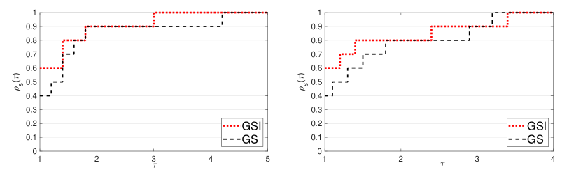
Figure 1: Performance profiles based on CPU time for medium scale problems with $n=100$ (left) and $n=200$ (right).

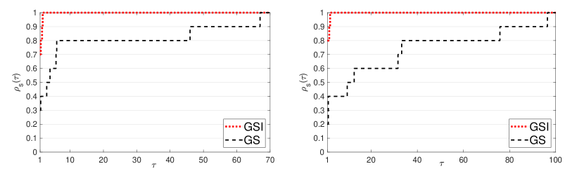
Figure 2: Performance profiles based on QP solver time for medium scale problems with $n=100$ (left) and $n=200$ (right).

6.3 Experiment 3. Large scale problems

In this experiment, we consider a set of nonsmooth test problems for which we set $n=500$ and $n=1000$. A description of the test problems is presented in Table 4. To the best of our knowledge, it is the first time that the GS method is applied to a set of problems having more than $200$ variables. Note that, due to heavy computational cost, an unreasonable amount of CPU time may be required for each run. Accordingly, we used Matlab Api for C++ language to manage the CPU time for the considered large scale problems.

Fig. 3 and Fig. 4 show results for problems with $500$ and $1000$ variables. As Fig. 3 demonstrates, at $70\%$ of the problems having $500$ variables, the GSI method used less CPU time than the GS method. In addition, Fig. 3 also demonstrates the superiority of the GSI method over the GS method for problems with $1000$ variables. It can be seen from Fig. 4 that, the proposed method has a remarkable potential to reduce the CPU time consumed by the QP solver. Thus, in the problems for which the QP (9) is a demanding part of the GS method, the GSI method is a more desirable choice.

Table 4: List of test problems for Experiment 3.

Problem	Name	Function Type	Ref.
1	Titled Norm Function	Convex	BFGS
2	A Convex Partly Smooth Function	Convex	BFGS
3	MAXQ	Convex	Haarala
4	Chained LQ	Convex	Haarala
5	Nesterov’s Chebyshev-Rosenbrock Function1	Nonconvex	BFGS
6	Nesterov’s Chebyshev-Rosenbrock Function2	Nonconvex	BFGS
7	Chained Mifflin 2	Nonconvex	Haarala
8	Chained Crescent I	Nonconvex	Haarala
9	Chained Crescent II	Nonconvex	Haarala
10	A Nonconvex Partly Smooth Function.	Nonconvex	BFGS

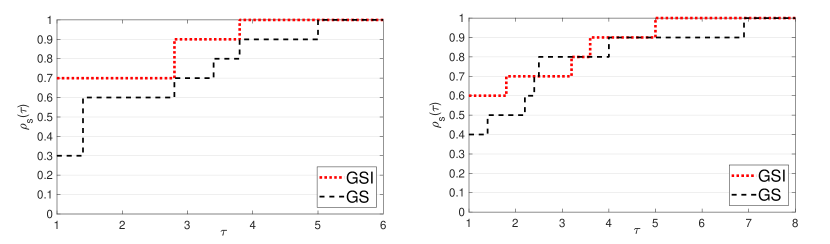
Figure 3: Performance profiles based on CPU time for large scale problems with $n=500$ (left) and $n=1000$ (right).

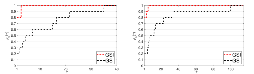
Figure 4: Performance profiles based on QP solver time for large scale problems with $n=500$ (left) and $n=1000$ (right).

7 Conclusion

In this article, by introducing the Ideal direction as an alternative of the approximate $\epsilon$-steepest descent direction, we reduced the need of solving quadratic subproblem in the GS method. We have shown that, Ideal directions are easy to compute and a nonzero Ideal direction can make a substantial reduction in the objective function. Furthermore, we showed that by using Ideal directions, not only is there no need to consider the quadratic subproblem in the smooth regions, but also it can be an efficient search direction when the method starts to track a nonsmooth curve towards a stationary point. We studied the convergence of the proposed method and we proved that using Ideal directions preserves the global convergence property of the GS method. Furthermore, by using limited backtracking Armijo line search and under some moderate assumptions, we proposed an upper bound for the number of serious iterations in the GSI algorithm. We presented numerical results using small, medium and large scale nonsmooth test problems. Our numerical results clearly demonstrate that, the GSI method inherits robustness from the GS method and it is a significant enhancement in reducing the number of quadratic subproblems.

References

• (1) Mäkelä, M.M., Neittaanmäki, P.: Nonsmooth optimization: Analysis and algorithms with applications to optimal control. Singapore: World Scientific Publishing Co. (1992)
• (2) Nikolova, M.: Minimizers of cost-functions involving nonsmooth data-fidelity terms. application to the processing of outliers. SIAM Journal on Numerical Analysis 40(3), 965–994 (2002)
• (3) Astorino, A., Gaudioso, M.: Polyhedral separability through successive LP. J. Optim. Theory Appl 112(2), 265–293 (2002)
• (4) Lavor, C., Liberti, L., Maculan, N.: Molecular distance geometry problem (2nd ed.). Springer (2009)
• (5) Witten, I.H., Frank, E.: Data mining: Practical machine learning tools and techniques (2nd ed.). Elsevier Inc (2005)
• (6) Clarke, F.H.: Optimization and nonsmooth analysis. SIAM (1990)
• (7) Kiwiel, K.C.: Methods of descent for nondifferentiable optimization. Springer-Verlag (1985)
• (8) Shor, N.Z.: Minimization methods for non-differentiable functions. Springer (1985)
• (9) Hiriart-Urruty, J.B., chal, C.L.: Convex Analysis and Minimization Algorithms I. A Series of Comprehensive Studies in Mathematics. Springer-Verlag (1993)
• (10) Hiriart-Urruty, J.B., chal, C.L.: Convex Analysis and Minimization Algorithms II. A Series of Comprehensive Studies in Mathematics. Springer-Verlag (1993)
• (11) Uryas’ev, S.P.: New variable metric algorithms for nondifferentiable optimization problems. J. Optim. Theory Appl 71, 359–388 (1991)
• (12) Vlček, J., Lukšan, L.: Globally convergent variable metric method for nonconvex nondifferentiable unconstrained minimization. J. Optim. Theory Appl 111(2), 407–430 (2001)
• (13) Bagirov, A.M., Jin, L., Karmitsa, N., Al Nuaimat, A., Sultanova, N.: A subgradient method for nonconvex nonsmooth optimization. J. Optim. Theory Appl 157, 416–435 (2013)
• (14) Mahdavi-Amiri, N., Yousefpour, R.: An effective nonsmooth optimization algorithm for locally Lipschitz functions. J. Optim. Theory Appl 155(1), 180–195 (2012)
• (15) Nesterov, Y.: Primal-dual subgradient methods for convex problems. Math. Program 120(1), 221–259 (2009)
• (16) Bagirov, A.M., Ganjehlou, A.N.: A quasisecant method for minimizing nonsmooth functions. Optim. Methods Softw 25(1), 3–18 (2010)
• (17) Haarala, M., Miettinen, K., Mäkelä, M.M.: New limited memory bundle method for large-scale nonsmooth optimization. Optim. Methods Softw 19(6), 673–692 (2004)
• (18) Lukšan, L., Vlček, J.: A bundle-Newton method for nonsmooth unconstrained minimization. Math. Program 83(1), 373–391 (1998)
• (19) Burke, J.V., Lewis, A.S., Overton, M.L.: A robust gradient sampling algorithm for nonsmooth, nonconvex optimization. SIAM J. Optim 15(3), 751–779 (2005)
• (20) Burke, J.V., Curtis, F.E., Lewis, A.S., Overton, M.L., Simões, L.E.A.: Gradient sampling methods for nonsmooth optimization. arXiv : 1804.11003 (2018)
• (21) Kiwiel, K.C.: Convergence of the gradient sampling algorithm for nonsmooth nonconvex optimization. SIAM J. Optim 18(2), 379–388 (2007)
• (22) Kiwiel, K.C.: A nonderivative version of the gradient sampling algorithm for nonsmooth nonconvex optimization. SIAM J. Optim 20(4), 1983–1994 (2010)
• (23) Curtis, F.E., Que, X.: An adaptive gradient sampling algorithm for nonconvex nonsmooth optimization. Optim. Methods Softw 28(6), 1302–1324 (2013)
• (24) Nocedal, J., Wright, S.J.: Numerical Optimization, second edition. Springer (2006)
• (25) Curtis, F.E., Overton, M.L.: A sequential quadratic programming algorithm for nonconvex, nonsmooth constrained optimization. SIAM J. Optim 22(2), 474–500 (2012)
• (26) Helou, E.S., Santos, A.S., Simões, L.E.A.: On the local convergence analysis of the gradient sampling method for finite max-functions. J. Optim. Theory Appl 175(1), 137–157 (2017)
• (27) Bagirov, A., Karmitsa, N., Mäkelä, M.M.: Introduction to nonsmooth optimization. Springer (2014)
• (28) Evans, L.C., Gariepy, R.F.: Measure theory and fine properties of functions, Revised Edition. CRC Press (1992)
• (29) Rockafellar, R.T., Wets, R.J.B.: Variational analysis. Springer (2004)
• (30) Rockafellar, R.T.: Convex Analysis. Princeton University Press (1970)
• (31) Bazaraa, M.S., Sherali, H.D., Shetty, C.M.: Nonlinear Programming. John Wiley & Sons, Inc. (2006)
• (32) Ehrgott, M.: Multicriteria Optimization. Springer (2005)
• (33) Lukšan, L., Vlček, J.: Test problems for nonsmooth unconstrained and linearly constrained optimization. Tech. rep., Institute of Computer Science, Academy of Sciences of the Czech Republic (2000)
• (34) Skaaja, M.: Limited memory BFGS for nonsmooth optimization. Master’s thesis, New York University (2010)
• (35) Lukšan, L., Tcma, M., Siska, M., Vlček, J., Ramesova, N.: Ufo 2002. interactive system for universal functional optimization. Tech. rep., Institute of Computer Science, Academy of Sciences of the Czech Republic (2002)
• (36) Grothey, A.: Decomposition methods for nonlinear nonconvex optimization problems. Ph.D. thesis, University of Edinburgh (2001)
• (37) Dolan, E., Moré, J.: Benchmarking optimization software with performance profiles. Math. Program 91(2), 201–213 (2002)
• (38) Lewis, A.S., Overton, M.L.: Nonsmooth optimization via BFGS URL https://cs.nyu.edu/overton/papers/nonsmoothalg.html