Dynamic Face Video Segmentation via Reinforcement Learning
Abstract
00footnotetext: †Corresponding author.00footnotetext: ∗Yujiang Wang conducted this research during his internship at Samsung AI Center, Cambridge and Nara Institute of Science and TechnologyFor real-time semantic video segmentation, most recent works utilised a dynamic framework with a key scheduler to make online key/non-key decisions. Some works used a fixed key scheduling policy, while others proposed adaptive key scheduling methods based on heuristic strategies, both of which may lead to suboptimal global performance. To overcome this limitation, we model the online key decision process in dynamic video segmentation as a deep reinforcement learning problem and learn an efficient and effective scheduling policy from expert information about decision history and from the process of maximising global return. Moreover, we study the application of dynamic video segmentation on face videos, a field that has not been investigated before. By evaluating on the 300VW dataset, we show that the performance of our reinforcement key scheduler outperforms that of various baselines in terms of both effective key selections and running speed. Further results on the Cityscapes dataset demonstrate that our proposed method can also generalise to other scenarios. To the best of our knowledge, this is the first work to use reinforcement learning for online key-frame decision in dynamic video segmentation, and also the first work on its application on face videos.
1 Introduction
In computer vision, semantic segmentation is a computationally intensive task which performs per-pixel classification on images. Following the pioneering work of Fully Convolutional Networks (FCN) [25], tremendous progress has been made in recent years with the propositions of various deep segmentation methods [5, 2, 52, 59, 24, 8, 22, 34, 6, 58, 30]. To achieve accurate result, these image segmentation models usually employ heavy-weight deep architectures and additional steps such as spatial pyramid pooling [59, 6, 5] and multi-scaled paths of inputs/features [7, 58, 23, 5, 4, 22, 35], which further increase the computational workload. For real-time applications such as autonomous driving, video surveillance, and facial analysis [49], it is impractical to apply such methods on a per-frame basis, which will result in high latency intolerable to those applications. Therefore, acceleration becomes a necessity for these models to be applied in real-time video segmentation.
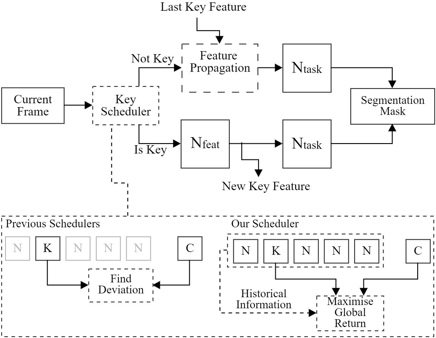
Various methods [40, 64, 54, 20, 16, 29, 17, 31, 11] have been proposed to accelerate video segmentation. Because adjacent frames in a video often share a large proportion of similar pixels, most of these works utilise a dynamic framework which separates frames into key and non-key frames and produce their segmentation masks differently. As illustrated in Fig. 1 (up), a deep image segmentation model is divided into a heavy feature extraction part and a light task-related part . To produce segmentation masks, key frames would go through both and , while a fast feature interpolation method is used to obtain features for the non-key frames by warping ’s output on the last key frame (LKF), thus to avoid the heavy cost of running on every frame. On top of that, a key scheduler is used to predict whether an incoming frame should be a key or non-key frame.
As an essential part of dynamic video segmentation, decisions made by the key scheduler could significantly affect the overall performance [20, 54, 62] of the video segmentation framework. However, this topic is somewhat underexplored by the community. Recent works have either adopted a fixed key scheduler [29, 64, 17, 16], or proposed adaptive schedulers [54, 20, 62] which are trained to heuristically predict similarities (or deviations) between two video frames. Those key schedulers lack awareness of the global video context and can lead to suboptimal performance in the long run.
To overcome this limitation, we propose to apply Reinforcement Learning (RL) techniques to expose the key scheduler to the global video context. Leveraging additional expert information about decision history, our scheduler is trained to learn key-decision policies that maximise the long-term returns in each episode, as shown in Fig. 1 (bottom).
We further study the problem of dynamic face video segmentation with our method. Comparing to semantic image/video segmentation, segmentation of face parts is a less investigated field [13, 61, 18, 45, 32, 50, 39, 55, 19, 12], and there are fewer works on face segmentation in videos [49, 37]. Existing works either used engineered features [18, 45, 50, 39, 55, 19], or employed outdated image segmentation models like FCN [25] on a per-frame basis [32, 37, 49] without a dynamic acceleration mechanism. Therefore, we propose a novel real-time face segmentation system utilising our key scheduler trained by Reinforcement Learning (RL).
We evaluate the performances of the proposed method on the 300 Videos in the Wild (300VW) dataset [41] for the task of real-time face segmentation. Comparing to several baseline approaches, we show that our reinforcement key scheduler can make more effective key-frame decisions at the cost of fewer resource. Through further experiment conducted on the Cityscapes dataset [10] for the task of semantic urban scene understanding, we demonstrate that our method can also generalise to other scenarios.
2 Related works
Semantic image segmentation Fully Convolutional Networks (FCN) [25] is the first work to use fully convolutional layers and skip connections to obtain pixel-level predictions for image segmentation. Subsequent works have made various improvements, including the usage of dilated convolutions [4, 5, 6, 56, 57], encoder-decoder architecture [2, 22, 8], Conditional Random Fields (CRF) for post-processing [60, 4, 5], spatial pyramid pooling to capture multi-scale features [59, 5, 6] and Neural Architecture Search (NAS) [65] to search for the best-performing architectures [3, 24]. Nonetheless, such models usually require intensive computational resources, and thus may lead to unacceptably high latency in video segmentation.
Dynamic video segmentation Clockwork ConvNet [40] promoted the idea of dynamic segmentation by fixing part of the network. Deep Feature Flow (DFF) [64] accelerated video recognition by leveraging optical flow (extracted by FlowNet [63, 15] or SpyNet [36]) to warp key-frame features. Similar ideas are explored in [54, 17, 31, 11]. Inter-BMV [16] used block motion vectors in compressed videos for acceleration. Mahasseni et al. [26] employed convolutions with uniform filters for feature interpolation, while Li et al. [20] used spatially-variant convolutions instead. Potential interpolation architectures were searched in [29].
On the other hand, studies of key schedulers are comparatively rare. Most existing works adopted fixed key schedulers [29, 64, 17, 16], which is inefficient for real-time segmentation. Mahasseni et al. [26] suggested a budget-aware, LSTM-based key selection strategy trained with reinforcement learning, which is only applicable for offline scenarios. DVSNet [54] proposed an adaptive key decision network based on the similarity score between the interpolated mask and the key predictions, i.e., low similarity scores leading to new keys and vice versa. Similary, Li et al. [20] introduced a dynamic key scheduler trained to predict the deviations between two video frames by the inconsistent low-level features, and [62] proposed to adaptively select key frames depending on the pixels with inconsistent temporal features. Those adaptive key schedulers only consider deviations between two frames, and therefore lack understandings of global video context, leading to suboptimal performances.
Semantic face segmentation Semantic face parts segmentation received far less attention than that of image/video segmentation. Early works on this topic mostly used engineered features [18, 45, 50, 39, 55, 19] and were designed for static images. Saito et al. [37] employed graphic cut algorithm to refine the probabilistic maps from a FCN trained with augmented data. In [32], a semi-supervised data collection approach was proposed to generate more labelled facial images with random occlusions to train FCN. Recently, Wang et al. [49] integrated Conv-LSTM [53] with FCN [25] to extract face masks from video sequence, while the run-time speed did not improve. None of the se works considered to adopt video dynamics for accelerations, and we are the first to do so for real-time face segmentation.
Reinforcement learning In model-free Reinforcement Learning (RL), an agent receives a state at each time step from the environment, and learns a policy with parameters that guides the agent to take an action to maximise the cumulative rewards . RL has demonstrated impressive performance on various fields such as robotics and complicated strategy games [21, 43, 28, 48, 42, 47]. In this paper, we show that RL can be seamlessly applied to online key decision problem in real-time video segmentation, and we chose the policy gradient with reinforcement [51] to learn , where gradient ascend was used for maximising the objective function .
3 Methodology
3.1 System Overview
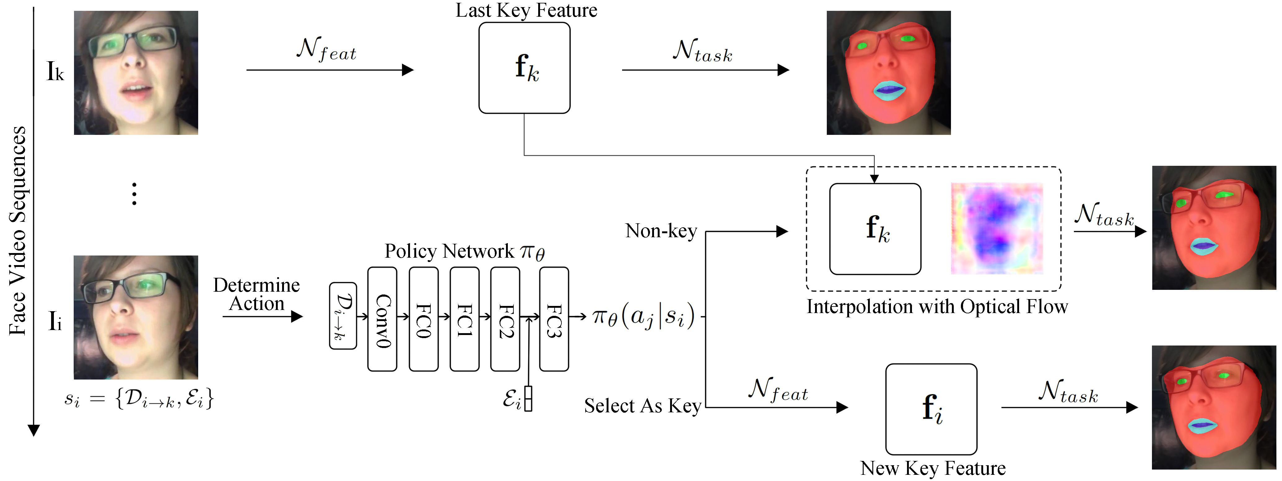
Our target is to develop an efficient and effective key scheduling policy for the dynamic video segmentation system. To this end, we use Deep Feature Flow [64] as the feature propagation framework, in which the optical flow is calculated by a light-weight flow estimation model such as FlowNet [63, 15] or SpyNet [36]. Specifically, an image segmentation model can be divided into a time-consuming feature extraction module and a task specified module . We denote the last key frame as and its features extracted by as , i.e., . For an incoming frame , if it is a key frame, the feature is and the segmentation mask is ; if not, instead of using the resource-intensive module for feature extraction, its feature will be propagated by a feature interpolation function , which involves the flow field from to , the scale field from to , and key frame feature , hence the predicted mask becomes . Please check [64] for more details on the feature propagation process.
On top of the DFF framework, we design a light-weight policy network to make online key predictions. The state at frame consists of two parts, the deviation information which describes the differences between and , and the expert information regarding key decision history (see Section 3.2 for details), i.e., . Feeding as input, the policy network outputs the action probabilities where and (we define for non-key action and for the key one). For an incoming frame , if where is a threshold, it will be identified as a key frame, vice versa. In general, key action will lead to a segmentation mask with better quality than the ones given by action .
In this work, we utilise the FlowNet2-s model [15] as the optical flow estimation function . DVSNet [54] has shown that the high-level features from FlowNet models contain sufficient information about the deviations between two frames, and it can also be easily fetched along with optical flow without additional cost. Therefore, we adopt the features of FlowNet2-s model for . It is worthwhile to notice that by varying properly, our key scheduler can be easily integrated into other dynamic segmentation frameworks [17, 20, 29, 16, 62] which do not use optical flow. Fig. 2 gives an overview of our system.
3.2 Training Policy Network
Network structure Our policy network comprises of one convolution layer and four fully connected (FC) layers. The FlowNet2-s feature is fed into the first convolution layer Conv0 with 96 channels, followed by FC layers (FC0, FC1 and FC2) with output size being 1024, 1024 and 128 respectively. Two additional channels containing expert information about decision history are concatenated to the output of FC2 layer. The first channel records the Key All Ratio (KAR), which is the ratio between the key frame and every other frames in decision history, while the second channel contains the Last Key Distance (LKD), which is the interval between the current and the last key frame. KAR provides information on the frequency of historical key selection, and LKD gives awareness about the length of continuous non-key decisions. Hence, the insertion of KAR and LKD extends the output dimension of FC2 to 130, while FC3 layer summarises all these information and gives action probabilities where , and stand for non-key and key action correspondingly.
Reward definition We use mean Intersection-over-Union (mIoU) as the metric to evaluate the segmentation masks. We denote the mIoU of from a non-key action as , the mIoU from key action as , and the reward at frame is defined in Eq. 1. Such definition encourages the scheduler to choose key action on the frames that would result in larger improvement over non-key action, and it also reduces the variances of mIoUs across the video.
| (1) | ||||
If no groundtruth is available (such that mIoU could not be calculated), we use the segmentation mask from key action as the pseudo groundtruth mask. In this case, the reward formulation is changed to Eq. 2, in which and denote the segmentation mask on frame from non-key action and key action respectively, and stands for the accuracy score with as the prediction and as the label.
| (2) | ||||
Constraining key selection frequency The constraints on key selection frequency are necessary in our task. Since a key action will generally lead to a better reward than a non-key one, the policy network inclines to make all-key decisions if no constraint is imposed on the frequency of key selection. In this paper, we propose a stop immediately exceeding the limitation approach. Particularly, for one episode consisting of frames , the agent starts from and explores continuously towards . At each time step, if the KAR in decision history has already surpassed a limit , the agent will stop immediately and thus this episode ends, otherwise, it will continue until reaching the last frame . By using this strategy, a policy network should limit the use of key decision to avoid an over-early stopping, and also learn to allocate the limited key budgets on the frames with higher rewards. By varying the KAR limit , we could train with different key decision frequencies.
Episode settings Real-time videos usually contains enormous number of high-dimensional frames, thus it is impractical to include all of them in one episode, due to the high computational complexity and possible huge variations across frames. For simplicity, we limit the length of one episode to 270 frames (9 seconds) for 300VW and 30 frames (snippet length) for Cityscapes respectively. We vary the starting frame during training to learn the global policies across videos. For each episode, we let the agent run times (with the aforementioned key constraint strategy) to obtain trials to reduce variances. The return of each episode can be expressed as , where is the starting frame index of the episode, and denotes the total step number at the trail (since agent may stop before steps), and refers to the reward of frame in trail. is the main objective function to optimise.
Auxiliary loss In addition to optimise the cumulative reward , we employ the entropy loss as in [27, 33] to promote the policy that retains high-entropy action posteriors so as to avoid over-confident actions. Eq. 3 shows the final objective function to optimise using policy gradient with reinforcement method [51].
| (3) | ||||
Epsilon-greedy strategy During training, agent may still fall into over-deterministic dilemmas with action posteriors approaching nearly 1, even though the auxiliary entropy loss have been added. To recover from such dilemma, we implement a simple strategy similar to epsilon-greedy algorithm for action sampling, i.e., in the cases that action probabilities exceed a threshold (such as 0.98), instead of taking action with probability , we use to stochastically pick action (and for picking action ).
4 Experiments
4.1 Datasets
We conducted experiments on two datasets: the 300 Videos on the Wild (300VW) dataset [41] and the Cityscapes dataset [10]. 300VW is used for evaluating the proposed real-time face segmentation system with the RL key selector. To the best of our knowledge, 300VW is the only publicly available face video dataset that provides per-frame segmentation labels. Therefore, to demonstrate the generality of our method, we also evaluate our method on Cityscapes [10], which is a widely used dataset for scene parsing, and thus we show how our RL key scheduler can generalise to other datasets and scenarios.
The 300VW dataset contains 114 face videos (captured at 30 FPS) with an average length of 64 seconds, all of which are taken in unconstrained environment. Following [49], we have cropped faces out of the video frames and generated the segmentation labels with facial skin, eyes, outer mouth and inner mouth for all the 218,595 frames. For experiment purpose, we divided the videos into three subject-independent parts, namely sets containing 51 / 51 / 12 videos. In detail, for training , we randomly picked 9,990 / 1,0320 / 2,400 frames from sets for training/validation/testing. To train , we randomly generate 32,410 / 4,836 / 6,671 key-current image pairs with a varying gap between 1 to 30 frames from sets for training/validation/testing. We intentionally excluded set for policy network learning, since this set has already been used to train and , instead, we used the full set (51 videos with 98,947 frames) for training and validating the RL key scheduler, and evaluated it on the full set (12 videos with 22,580 frames).
The Cityscapes dataset contains 2,975 / 500 / 1,525 annotated urban scene images as training/validation/testing set, while each annotated image is the frame of a 30-frame (1.8 seconds) video snippet. To ensure a fair comparison on this dataset, we have adopted the same preliminary models ( and ) and the model weights provided by the authors of DVSNet [54], such that we only re-trained the proposed RL key schedulers using the Cityscapes training snippets. Following DVSNet [54], our method and the baselines are evaluated on the validation snippets, where the initial frame is set as key and performances are measured on the annotated frame.
4.2 Experimental Setup
Evaluation metric We employed the commonly used mean Intersection-over-Union (mIoU) as the evaluation metric. For the performance evaluation of different key schedulers, we measure: 1. the relationship between Average Key Intervals (AKI) and mIoU, as to demonstrate the effectiveness of key selections under different speed requirements, and 2. the relationship between the actual FPS and mIoU.
Training preliminary networks On 300VW, we utilised the state-of-the-art Deeplab-V3+ architecture [8] for image segmentation model , and we adopted the FlowNet2-s architecture [15] as the implementation of flow estimation function . For training , we initialised the weights using the pre-trained model provided in [8] and then fine-tuned it. We set the output stride and decoder output stride to 16 and 4, respectively. We divided into and , where the output of is the posterior for each image pixel, we then fine-tuned the FlowNet2-s model as suggested in [64] by freezing and . Also, we used the pre-trained weights provided in [15] as the starting point of training . The input sizes for and are both set to 513*513.
On Cityscapes, we have adopted identical and architectures as DVSNet [54] and directly use the weights provided by the authors, such that we only re-trained the proposed policy key scheduler. Besides, we have also adopted the frame division strategy from DVSNet and have divided the frame into four individual regions. We refer interested readers to [54] for more details.
Reinforcement learning settings For state , following DVSNet [54], we leveraged the features from the Conv6 layer of the FlowNet2-s model as the deviation information , and we obtained the expert information from the last 90 decisions. During the training of policy network, , and were frozen to avoid unnecessary computations. We chose RMSProp [46] as the optimiser and set the initial learning rate to 0.001. The parameters in Eq. 3 were set to 0.14. We empirically decided the discount factor to be 1.0, as the per frame performance was equally important in our task. The value of epsilon in epsilon-greedy strategy was set to 0.98. During training, we set the threshold value for determining the key action to 0.5. We used the reward formulation as defined in Eq. 1 for 300VW. For Cityscapes, the modified reward as defined in Eq. 2 was used because most frames in the Cityscapes dataset are not annotated. The maximum length of each episode was set to 270 frames (9 seconds) for 300VW and 30 frames (snippet length) for Cityscapes respectively, and we repeated a relatively large number of 32 trials for each episode with a mini-batch size of 8 episodes for back-propagation in . We trained each model for 2,400 episodes and validated the performances of checkpoints on the same set. We also varied the KAR limit to obtain policy networks with different key decision tendencies.
Baseline comparison We compared our method with three baseline approaches on both datasets: (1) The adaptive key decision model DVSNet [54]; (2) The adaptive key scheduler using flow magnitude difference in [54]; (3) Deep Feature Flow (DFF) with a fixed key scheduler as in [64]. We utilised the same implementations and settings for the baselines as described in DVSNet paper, and we refer the readers to [54] for details. Note that for the implementation of DVSNet on Cityscapes, we directly used the model weights provided by the authors, but we have re-trained the DVSNet model on 300VW. For our method, to obtain key decisions with different Average Key Intervals, we have trained multiple models with various KAR limit , and also varied the key threshold values of those models.
Implementation We implemented our method in Tensorflow [1] framework. Experiments were run on a cluster with eight NVidia 1080 Ti GPUs, and it took approximately 2.5 days to train a RL model per GPU.
| Model | Eval Scales | mIoU(%) | FPS |
| FCN (VGG16) | N/A | 63.54 | 45.5 |
| Deeplab-V2 (VGG16) | N/A | 65.80 | 3.44 |
| Deeplab-V3+ (Xception-65) | 1.0 | 68.25 | 24.4 |
| 1.25, 1.75 | 68.98 | 6.4 | |
| Deeplab-V3+ (MobileNet-V2) | 1.0 | 67.07 | 58.8 |
| 1.25, 1.75 | 68.20 | 21.7 | |
| Deeplab-V3+ (ResNet-50) | 1.0 | 67.50 | 33.3 |
| 1.25, 1.75 | 69.61 | 10.1 | |
| FlowNet2-s | N/A | 64.13 | 153.8 |
4.3 Results
Preliminary networks on 300VW We evaluated five image segmentation models on 300VW dataset: FCN [25] with VGG16 [44] architecture, Deeplab-V2 [5] of VGG16 version, the Deeplab-V3+ [8] with Xception-65 [9] / MobileNet-V2 [38] / RestNet-50 [14] backbones. We have also tested two different eval scales (refer [8] for details) for Deeplab-V3+ model. As can be seen from Table 1, Deeplab-V3+ with ResNet-50 backbone and multiple eval scales (1.25 and 1.75) has achieved the best mIoU with an acceptable FPS, therefore we selected it for our segmentation model . Its feature extraction part was used to extract key frame feature in key-current images pairs during the training of FlowNet2-s [15] model , whose performance was evaluated by the interpolation results on current frames. From Table 1 we can discover that the interpolation speed with is generally much faster than those segmentation models at the cost of a slight drop in mIoU (from 69.61% to 64.13%). Under live video scenario, the loss of accuracy can be effectively remedied by a good key scheduler.
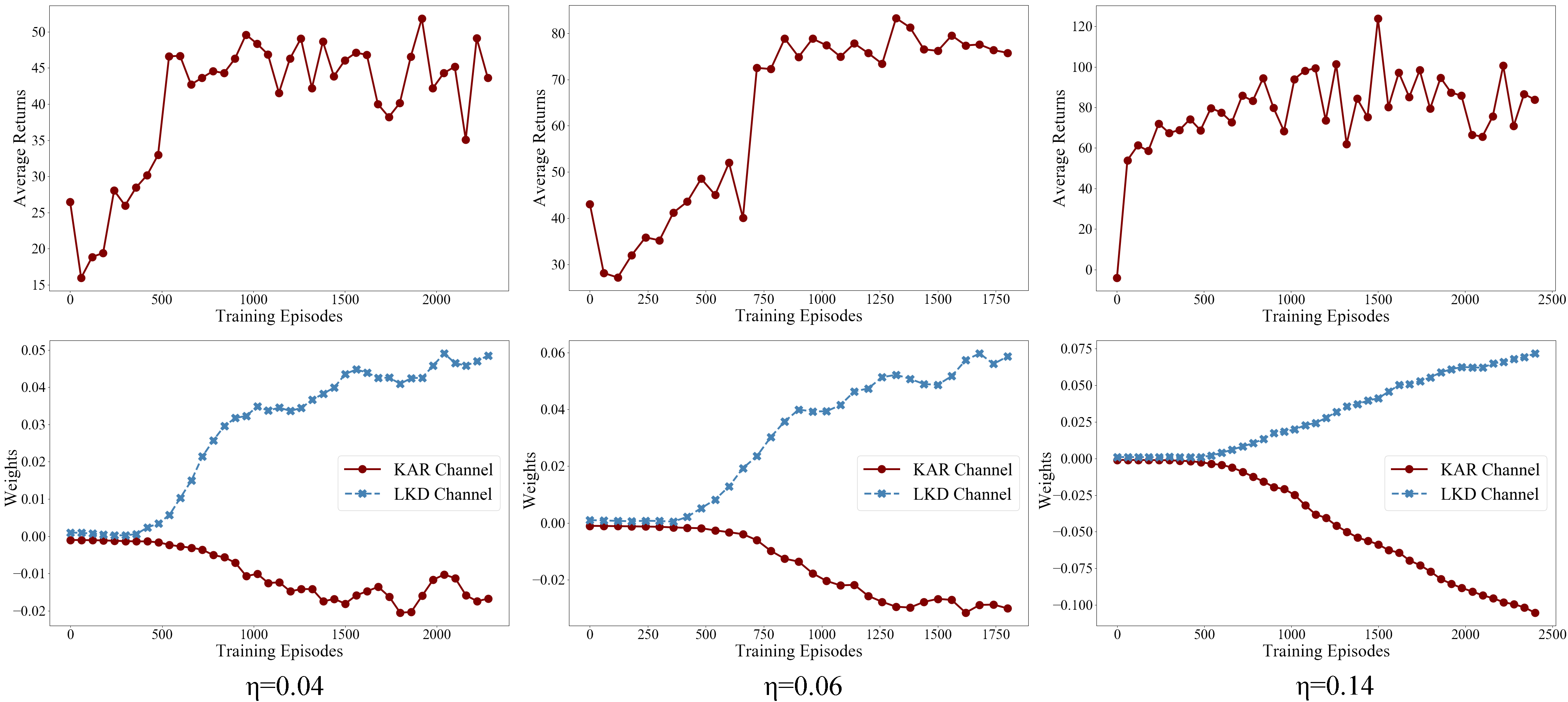
RL training visualisation on 300VW In the upper row of Fig. 3, we demonstrate the average return during RL training with different KAR limits (0.04, 0.06, 0.14) on 300VW dataset. It can be seen that even though we select the starting frames of each episode randomly, those return curves still exhibit a generally increasing trend despite several fluctuations. This validates the effectiveness of our solutions for reducing variances and stabilising gradients, and it also verifies that the policy is improving towards more rewarding key actions. Besides, as the value of increases and allows for more key actions, the maximum return that each curve achieves also becomes intuitively higher.
We also visualised the influences of two expert information KAR and LDK by plotting their weights in during RL training on 300VW. In the bottom row of Fig. 3, we have plotted the weights of the two channels in that received KAR and LDK as input and contributed to the key posteriors , and we can observe that the weights of the LDK channel show a globally rising trend, while that of the KAR channel decrease continuously. Such trends indicate that the KAR/LDK channels become increasingly important in key decisions as training proceeds, since a large LDK value (or a small KAR) will encourage to take key action. This observation is consistent with the proposed key constraint strategy. Furthermore, we can also imply that the key scheduler relies more on the LDK channel than the KAR with a lower like 0.04, conversely, KAR becomes more significant with a higher like 0.14.
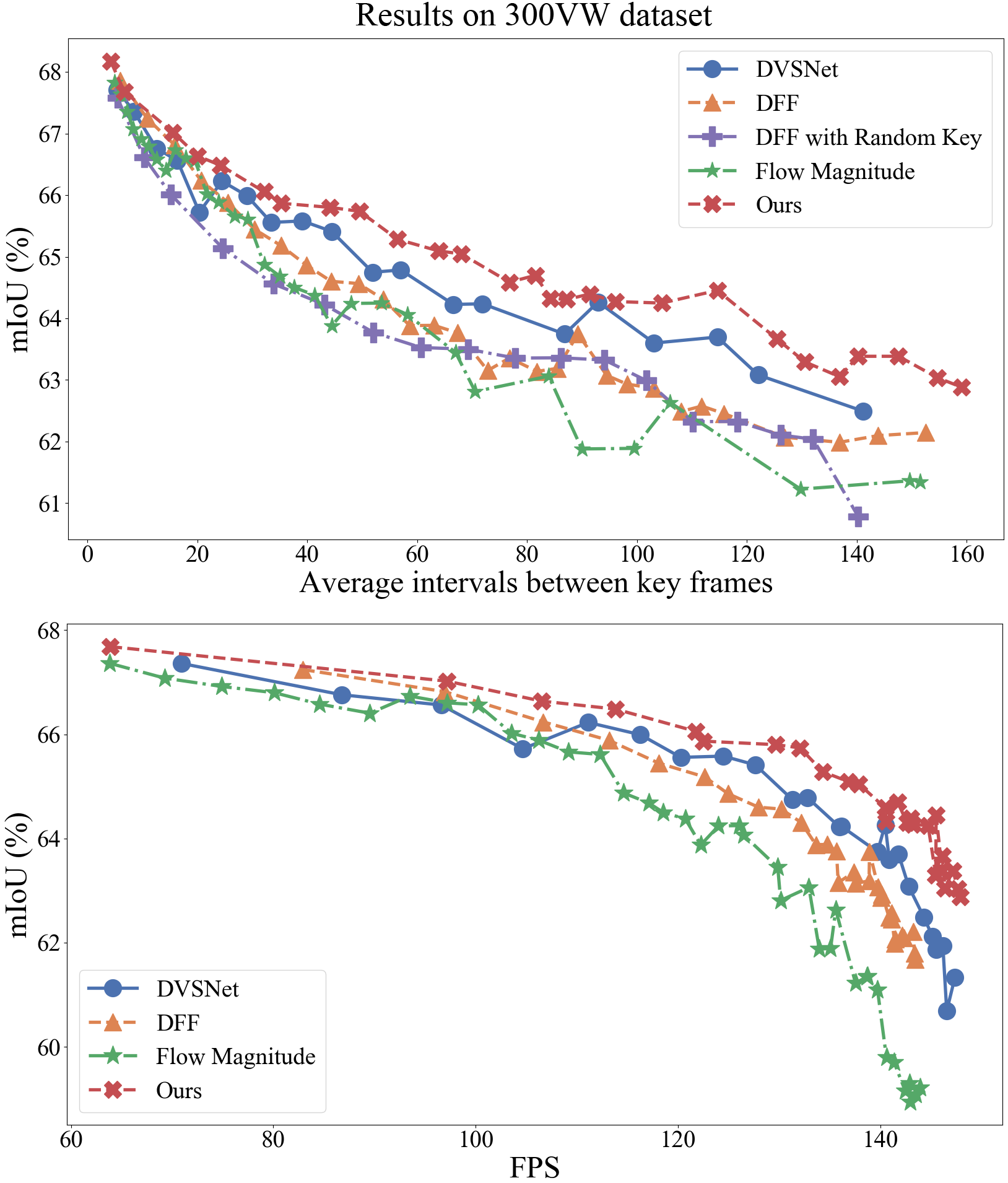
Performances evaluations The upper plot of Fig. 4 shows the Average Key Intervals (AKI) versus mIoU of various key selectors on the 300VW dataset and the bottom plot depicts the corresponding FPS versus mIoU curves. Note that in the AKI vs. mIoU graph, we include two versions of DFF: the one with fixed key intervals and the variant with randomly selected keys. We can easily see that our key scheduler have shown superior performance than others in terms of both effective key selections and the actual running speed. Although the performance of all methods are similar for AKI less than 20, this is to be expected as the performance degradation on non-key frames can be compensated by dense key selections. Our method starts to show superior performance when the key interval increases beyond 25, where our mIoUs are consistently higher than that of other methods and decreases slower as the key interval increases.
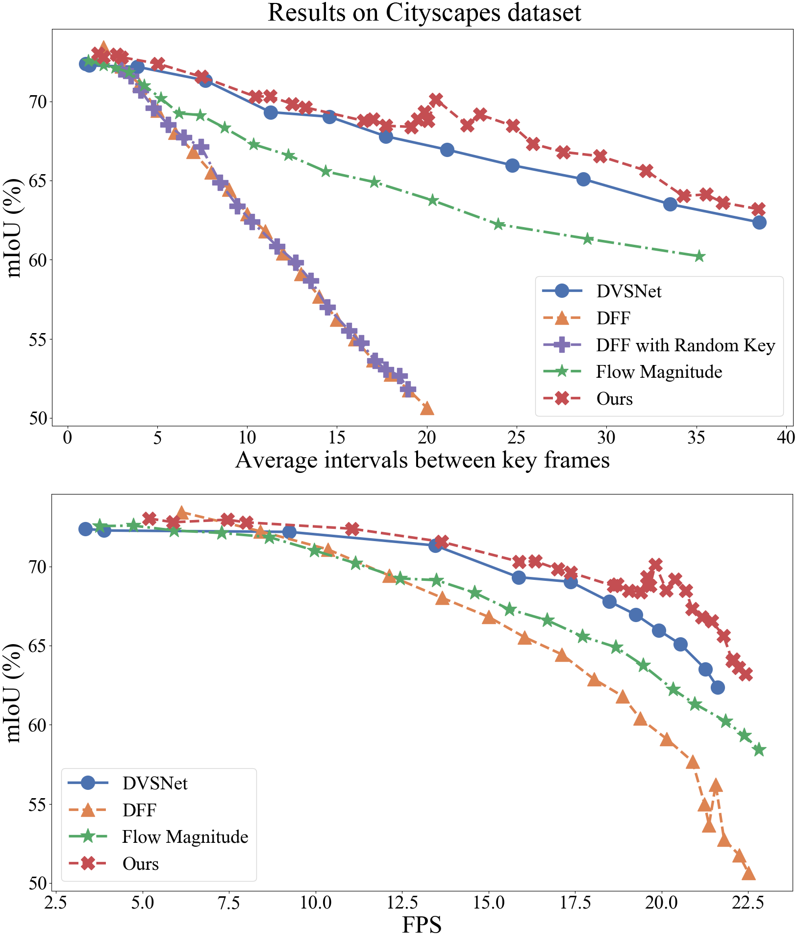
The evaluation results on Cityscapes can be found in Fig. 5, which demonstrates a similar trend with those results on 300VW and therefore validates the generality of our RL key scheduler to other datasets and tasks. However, it should be noted that, in the case of face videos, selecting key frames by a small interval () does not significantly affect the performance, which is not the same as in the autonomous driving scenarios of Cityscapes. This could be attributed to the fact that variations between consecutive frames in face videos are generally less than those in autonomous driving scenes. As a result, we can gain more efficiency benefit when using key scheduling policy with relatively large interval for dynamic segmentation of face video.
4.4 Visualising Key Selections
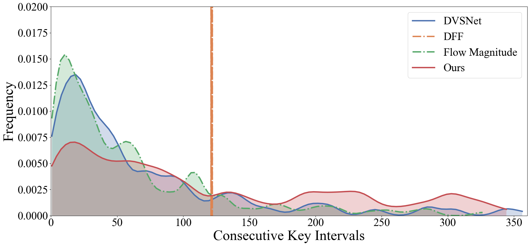
To better understand why our RL-based key selection method outperforms the baselines, we visualise the distribution of intervals between consecutive keys (CKI) based on the key selections made by all evaluated methods. Without loss of generality, Fig. 6 shows the density curves plotted from the experiment on 300VW dataset at AKI=121. As DFF uses a fixed key interval, its CKI distribution takes the shape of a single spike in the figure. In contrast, the CKI distribution given by our method has the flattest shape, meaning that the key frames selected by our method are more unevenly situated in the test videos. Noticeably, there are more cases of large gaps (>200) between neighbouring keys selected by our method than by others. This indicates our method could better capture the dynamics of the video and only select keys that have larger global impact to the segmentation accuracy.
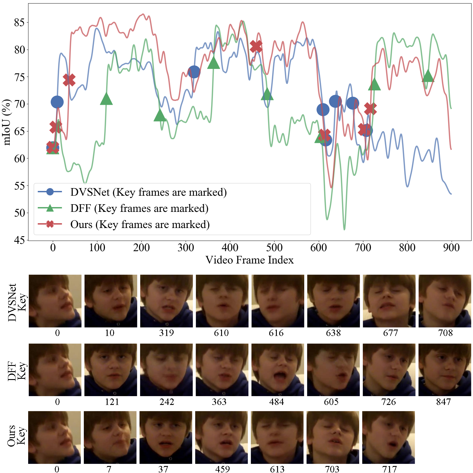
In addition, we also visualise the key frames selected by our method, DFF and DVSNet on a 30-second test video in Fig. 7 to provide insight on how the key selections can affect the mIoU. We can observe from this figure that the key frames selected by our method can better compensate for the loss of accuracy and retain higher mIoU over longer span of frames (such as frame 37 and 459), while those selected by DFF (fixed scheduler) are less flexible and the compensation to mIoU loss is generally worse than ours. Comparing DVSNet with ours, we can see that 1) our method can give key decisions with more stable non-key mIoUs (frames 37, 459 and 713), and 2) on hard frames such as frames 600 to 750, our reinforcement key scheduler has also made better compensations to performance loss with less key frames. These observations demonstrate the benefits brought by reinforcement learning, which is to learn key-decision policies from the global video context.
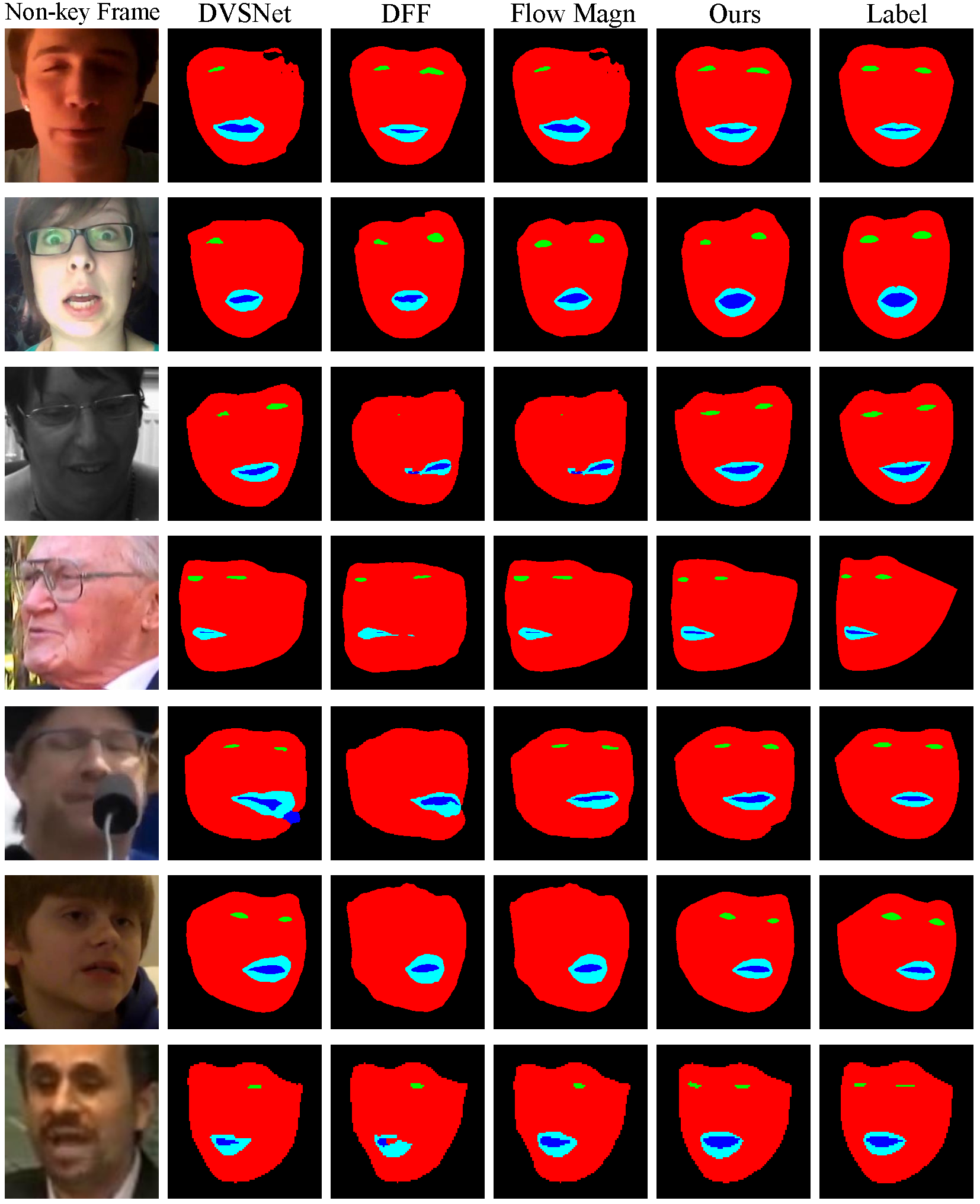
Last but not least, in Fig. 8, we plot the segmentation masks generated by different methods on several non-key frames during the experiment on 300VW dataset (AKI=121). It can be seen that DFF with fixed key schedulers usually leads to low-quality masks with missing facial components, while the DVSNet and the Flow Magnitude methods have shown better but still not satisfying results. In contrast, our method has produced non-key masks with the best visual qualities, which further validate the effectiveness of the proposed key schedulers.
5 Conclusions
In this paper, we proposed to learn an efficient and effective key scheduler via reinforcement learning for dynamic face video segmentation. By utilising expert information and appropriately designed training strategies, our key scheduler achieves more effective key decisions than baseline methods at smaller computational cost. We also show the method is not limited to face video but could also generalise to other scenarios. By visualising the key selections made by our method, we try to explain why our key scheduler can make better selections than others. This is the first work to apply dynamic segmentation techniques with RL on real-time face videos, and it can be inspiring to future works on real-time face segmentation and on dynamic video segmentation.
Acknowledgements
The work of Yujiang Wang has been partially supported by China Scholarship Council (No. 201708060212) and the EPSRC project EP/N007743/1 (FACER2VM). The work of Yang Wu has been supported, in part, by Microsoft Research Asia through MSRA Collaborative Research 2019 Grant.
References
- [1] Martín Abadi, Ashish Agarwal, Paul Barham, Eugene Brevdo, Zhifeng Chen, Craig Citro, Greg S. Corrado, Andy Davis, Jeffrey Dean, Matthieu Devin, Sanjay Ghemawat, Ian Goodfellow, Andrew Harp, Geoffrey Irving, Michael Isard, Yangqing Jia, Rafal Jozefowicz, Lukasz Kaiser, Manjunath Kudlur, Josh Levenberg, Dan Mané, Rajat Monga, Sherry Moore, Derek Murray, Chris Olah, Mike Schuster, Jonathon Shlens, Benoit Steiner, Ilya Sutskever, Kunal Talwar, Paul Tucker, Vincent Vanhoucke, Vijay Vasudevan, Fernanda Viégas, Oriol Vinyals, Pete Warden, Martin Wattenberg, Martin Wicke, Yuan Yu, and Xiaoqiang Zheng. TensorFlow: Large-scale machine learning on heterogeneous systems, 2015. Software available from tensorflow.org.
- [2] Vijay Badrinarayanan, Alex Kendall, and Roberto Cipolla. Segnet: A deep convolutional encoder-decoder architecture for image segmentation. IEEE transactions on pattern analysis and machine intelligence, 39(12):2481–2495, 2017.
- [3] Liang-Chieh Chen, Maxwell D. Collins, Yukun Zhu, George Papandreou, Barret Zoph, Florian Schroff, Hartwig Adam, and Jonathon Shlens. Searching for efficient multi-scale architectures for dense image prediction. In NIPS, 2018.
- [4] Liang-Chieh Chen, George Papandreou, Iasonas Kokkinos, Kevin Murphy, and Alan L Yuille. Semantic image segmentation with deep convolutional nets and fully connected crfs. arXiv preprint arXiv:1412.7062, 2014.
- [5] Liang-Chieh Chen, George Papandreou, Iasonas Kokkinos, Kevin Murphy, and Alan L Yuille. Deeplab: Semantic image segmentation with deep convolutional nets, atrous convolution, and fully connected crfs. IEEE transactions on pattern analysis and machine intelligence, 40(4):834–848, 2018.
- [6] Liang-Chieh Chen, George Papandreou, Florian Schroff, and Hartwig Adam. Rethinking atrous convolution for semantic image segmentation. arXiv preprint arXiv:1706.05587, 2017.
- [7] Liang-Chieh Chen, Yi Yang, Jiang Wang, Wei Xu, and Alan L Yuille. Attention to scale: Scale-aware semantic image segmentation. In Proceedings of the IEEE conference on computer vision and pattern recognition, pages 3640–3649, 2016.
- [8] Liang-Chieh Chen, Yukun Zhu, George Papandreou, Florian Schroff, and Hartwig Adam. Encoder-decoder with atrous separable convolution for semantic image segmentation. In ECCV, 2018.
- [9] François Chollet. Xception: Deep learning with depthwise separable convolutions. In Proceedings of the IEEE conference on computer vision and pattern recognition, pages 1251–1258, 2017.
- [10] Marius Cordts, Mohamed Omran, Sebastian Ramos, Timo Rehfeld, Markus Enzweiler, Rodrigo Benenson, Uwe Franke, Stefan Roth, and Bernt Schiele. The cityscapes dataset for semantic urban scene understanding. In Proceedings of the IEEE conference on computer vision and pattern recognition, pages 3213–3223, 2016.
- [11] Raghudeep Gadde, Varun Jampani, and Peter V Gehler. Semantic video cnns through representation warping. In Proceedings of the IEEE International Conference on Computer Vision, pages 4453–4462, 2017.
- [12] Golnaz Ghiasi, Charless C Fowlkes, and C Irvine. Using segmentation to predict the absence of occluded parts. In BMVC, pages 22–1, 2015.
- [13] Umut Güçlü, Yağmur Güçlütürk, Meysam Madadi, Sergio Escalera, Xavier Baró, Jordi González, Rob van Lier, and Marcel AJ van Gerven. End-to-end semantic face segmentation with conditional random fields as convolutional, recurrent and adversarial networks. arXiv preprint arXiv:1703.03305, 2017.
- [14] Kaiming He, Xiangyu Zhang, Shaoqing Ren, and Jian Sun. Deep residual learning for image recognition. In Proceedings of the IEEE conference on computer vision and pattern recognition, pages 770–778, 2016.
- [15] Eddy Ilg, Nikolaus Mayer, Tonmoy Saikia, Margret Keuper, Alexey Dosovitskiy, and Thomas Brox. Flownet 2.0: Evolution of optical flow estimation with deep networks. In Proceedings of the IEEE Conference on Computer Vision and Pattern Recognition, pages 2462–2470, 2017.
- [16] Samvit Jain and Joseph E Gonzalez. Inter-bmv: Interpolation with block motion vectors for fast semantic segmentation on video. arXiv preprint arXiv:1810.04047, 2018.
- [17] Samvit Jain, Xin Wang, and Joseph Gonzalez. Accel: A corrective fusion network for efficient semantic segmentation on video. arXiv preprint arXiv:1807.06667, 2018.
- [18] Andrew Kae, Kihyuk Sohn, Honglak Lee, and Erik Learned-Miller. Augmenting crfs with boltzmann machine shape priors for image labeling. In Proceedings of the IEEE Conference on Computer Vision and Pattern Recognition, pages 2019–2026, 2013.
- [19] Kuang-chih Lee, Dragomir Anguelov, Baris Sumengen, and Salih Burak Gokturk. Markov random field models for hair and face segmentation. In Automatic Face & Gesture Recognition, 2008. FG’08. 8th IEEE International Conference on, pages 1–6. IEEE, 2008.
- [20] Yule Li, Jianping Shi, and Dahua Lin. Low-latency video semantic segmentation. In Proceedings of the IEEE Conference on Computer Vision and Pattern Recognition, pages 5997–6005, 2018.
- [21] Timothy P Lillicrap, Jonathan J Hunt, Alexander Pritzel, Nicolas Heess, Tom Erez, Yuval Tassa, David Silver, and Daan Wierstra. Continuous control with deep reinforcement learning. arXiv preprint arXiv:1509.02971, 2015.
- [22] Guosheng Lin, Anton Milan, Chunhua Shen, and Ian Reid. Refinenet: Multi-path refinement networks for high-resolution semantic segmentation. In Proceedings of the IEEE conference on computer vision and pattern recognition, pages 1925–1934, 2017.
- [23] Guosheng Lin, Chunhua Shen, Anton Van Den Hengel, and Ian Reid. Efficient piecewise training of deep structured models for semantic segmentation. In Proceedings of the IEEE Conference on Computer Vision and Pattern Recognition, pages 3194–3203, 2016.
- [24] Chenxi Liu, Liang-Chieh Chen, Florian Schroff, Hartwig Adam, Wei Hua, Alan Yuille, and Li Fei-Fei. Auto-deeplab: Hierarchical neural architecture search for semantic image segmentation. In CVPR, 2019.
- [25] Jonathan Long, Evan Shelhamer, and Trevor Darrell. Fully convolutional networks for semantic segmentation. In Proceedings of the IEEE Conference on Computer Vision and Pattern Recognition, pages 3431–3440, 2015.
- [26] Behrooz Mahasseni, Sinisa Todorovic, and Alan Fern. Budget-aware deep semantic video segmentation. In Proceedings of the IEEE Conference on Computer Vision and Pattern Recognition, pages 1029–1038, 2017.
- [27] Volodymyr Mnih, Adria Puigdomenech Badia, Mehdi Mirza, Alex Graves, Timothy Lillicrap, Tim Harley, David Silver, and Koray Kavukcuoglu. Asynchronous methods for deep reinforcement learning. In International conference on machine learning, pages 1928–1937, 2016.
- [28] Volodymyr Mnih, Koray Kavukcuoglu, David Silver, Alex Graves, Ioannis Antonoglou, Daan Wierstra, and Martin Riedmiller. Playing atari with deep reinforcement learning. arXiv preprint arXiv:1312.5602, 2013.
- [29] Vladimir Nekrasov, Hao Chen, Chunhua Shen, and Ian Reid. Architecture search of dynamic cells for semantic video segmentation. arXiv preprint arXiv:1904.02371, 2019.
- [30] Vladimir Nekrasov, Chunhua Shen, and Ian Reid. Light-weight refinenet for real-time semantic segmentation. arXiv preprint arXiv:1810.03272, 2018.
- [31] David Nilsson and Cristian Sminchisescu. Semantic video segmentation by gated recurrent flow propagation. In Proceedings of the IEEE Conference on Computer Vision and Pattern Recognition, pages 6819–6828, 2018.
- [32] Yuval Nirkin, Iacopo Masi, Anh Tran Tuan, Tal Hassner, and Gérard Medioni. On face segmentation, face swapping, and face perception. In 2018 13th IEEE International Conference on Automatic Face & Gesture Recognition (FG 2018), pages 98–105. IEEE, 2018.
- [33] Kunkun Pang, Mingzhi Dong, Yang Wu, and Timothy Hospedales. Meta-learning transferable active learning policies by deep reinforcement learning. arXiv preprint arXiv:1806.04798, 2018.
- [34] Adam Paszke, Abhishek Chaurasia, Sangpil Kim, and Eugenio Culurciello. Enet: A deep neural network architecture for real-time semantic segmentation. arXiv preprint arXiv:1606.02147, 2016.
- [35] Tobias Pohlen, Alexander Hermans, Markus Mathias, and Bastian Leibe. Full-resolution residual networks for semantic segmentation in street scenes. In Proceedings of the IEEE Conference on Computer Vision and Pattern Recognition, pages 4151–4160, 2017.
- [36] Anurag Ranjan and Michael J Black. Optical flow estimation using a spatial pyramid network. In Proceedings of the IEEE Conference on Computer Vision and Pattern Recognition, pages 4161–4170, 2017.
- [37] Shunsuke Saito, Tianye Li, and Hao Li. Real-time facial segmentation and performance capture from rgb input. In European Conference on Computer Vision, pages 244–261. Springer, 2016.
- [38] Mark Sandler, Andrew Howard, Menglong Zhu, Andrey Zhmoginov, and Liang-Chieh Chen. Mobilenetv2: Inverted residuals and linear bottlenecks. In CVPR, 2018.
- [39] Carl Scheffler and Jean-Marc Odobez. Joint adaptive colour modelling and skin, hair and clothing segmentation using coherent probabilistic index maps. In British Machine Vision Association-British Machine Vision Conference, number EPFL-CONF-192633, 2011.
- [40] Evan Shelhamer, Kate Rakelly, Judy Hoffman, and Trevor Darrell. Clockwork convnets for video semantic segmentation. In Computer Vision–ECCV 2016 Workshops, pages 852–868. Springer, 2016.
- [41] Jie Shen, Stefanos Zafeiriou, Grigoris G Chrysos, Jean Kossaifi, Georgios Tzimiropoulos, and Maja Pantic. The first facial landmark tracking in-the-wild challenge: Benchmark and results. In Proceedings of the IEEE International Conference on Computer Vision Workshops, pages 50–58, 2015.
- [42] Victor do Nascimento Silva and Luiz Chaimowicz. Moba: a new arena for game ai. arXiv preprint arXiv:1705.10443, 2017.
- [43] David Silver, Aja Huang, Chris J Maddison, Arthur Guez, Laurent Sifre, George Van Den Driessche, Julian Schrittwieser, Ioannis Antonoglou, Veda Panneershelvam, Marc Lanctot, et al. Mastering the game of go with deep neural networks and tree search. nature, 529(7587):484, 2016.
- [44] Karen Simonyan and Andrew Zisserman. Very deep convolutional networks for large-scale image recognition. arXiv preprint arXiv:1409.1556, 2014.
- [45] Brandon M Smith, Li Zhang, Jonathan Brandt, Zhe Lin, and Jianchao Yang. Exemplar-based face parsing. In Proceedings of the IEEE Conference on Computer Vision and Pattern Recognition, pages 3484–3491, 2013.
- [46] Tijmen Tieleman and Geoffrey Hinton. Lecture 6.5-rmsprop: Divide the gradient by a running average of its recent magnitude. COURSERA: Neural networks for machine learning, 4(2):26–31, 2012.
- [47] Oriol Vinyals, Igor Babuschkin, Junyoung Chung, Michael Mathieu, Max Jaderberg, Wojciech M Czarnecki, Andrew Dudzik, Aja Huang, Petko Georgiev, Richard Powell, et al. Alphastar: Mastering the real-time strategy game starcraft ii. DeepMind Blog, 2019.
- [48] Oriol Vinyals, Timo Ewalds, Sergey Bartunov, Petko Georgiev, Alexander Sasha Vezhnevets, Michelle Yeo, Alireza Makhzani, Heinrich Küttler, John Agapiou, Julian Schrittwieser, et al. Starcraft ii: A new challenge for reinforcement learning. arXiv preprint arXiv:1708.04782, 2017.
- [49] Yujiang Wang, Bingnan Luo, Jie Shen, and Maja Pantic. Face mask extraction in video sequence. International Journal of Computer Vision, pages 1–17, 2018.
- [50] Jonathan Warrell and Simon JD Prince. Labelfaces: Parsing facial features by multiclass labeling with an epitome prior. In Image Processing (ICIP), 2009 16th IEEE International Conference on, pages 2481–2484. IEEE, 2009.
- [51] Ronald J Williams. Simple statistical gradient-following algorithms for connectionist reinforcement learning. Machine learning, 8(3-4):229–256, 1992.
- [52] Zifeng Wu, Chunhua Shen, and Anton Van Den Hengel. Wider or deeper: Revisiting the resnet model for visual recognition. Pattern Recognition, 90:119–133, 2019.
- [53] SHI Xingjian, Zhourong Chen, Hao Wang, Dit-Yan Yeung, Wai-Kin Wong, and Wang-chun Woo. Convolutional lstm network: A machine learning approach for precipitation nowcasting. In Advances in neural information processing systems, pages 802–810, 2015.
- [54] Yu-Syuan Xu, Tsu-Jui Fu, Hsuan-Kung Yang, and Chun-Yi Lee. Dynamic video segmentation network. In Proceedings of the IEEE Conference on Computer Vision and Pattern Recognition, pages 6556–6565, 2018.
- [55] Yaser Yacoob and Larry S Davis. Detection and analysis of hair. IEEE transactions on pattern analysis and machine intelligence, 28(7):1164–1169, 2006.
- [56] Fisher Yu and Vladlen Koltun. Multi-scale context aggregation by dilated convolutions. arXiv preprint arXiv:1511.07122, 2015.
- [57] Fisher Yu, Vladlen Koltun, and Thomas Funkhouser. Dilated residual networks. In Proceedings of the IEEE conference on computer vision and pattern recognition, pages 472–480, 2017.
- [58] Hengshuang Zhao, Xiaojuan Qi, Xiaoyong Shen, Jianping Shi, and Jiaya Jia. Icnet for real-time semantic segmentation on high-resolution images. In Proceedings of the European Conference on Computer Vision (ECCV), pages 405–420, 2018.
- [59] Hengshuang Zhao, Jianping Shi, Xiaojuan Qi, Xiaogang Wang, and Jiaya Jia. Pyramid scene parsing network. In Proceedings of the IEEE conference on computer vision and pattern recognition, pages 2881–2890, 2017.
- [60] Shuai Zheng, Sadeep Jayasumana, Bernardino Romera-Paredes, Vibhav Vineet, Zhizhong Su, Dalong Du, Chang Huang, and Philip HS Torr. Conditional random fields as recurrent neural networks. In Proceedings of the IEEE International Conference on Computer Vision, pages 1529–1537, 2015.
- [61] Yisu Zhou, Xiaolin Hu, and Bo Zhang. Interlinked convolutional neural networks for face parsing. In International Symposium on Neural Networks, pages 222–231. Springer, 2015.
- [62] Xizhou Zhu, Jifeng Dai, Lu Yuan, and Yichen Wei. Towards high performance video object detection. In Proceedings of the IEEE Conference on Computer Vision and Pattern Recognition, pages 7210–7218, 2018.
- [63] Xizhou Zhu, Yujie Wang, Jifeng Dai, Lu Yuan, and Yichen Wei. Flow-guided feature aggregation for video object detection. In Proceedings of the IEEE International Conference on Computer Vision, pages 408–417, 2017.
- [64] Xizhou Zhu, Yuwen Xiong, Jifeng Dai, Lu Yuan, and Yichen Wei. Deep feature flow for video recognition. In Proceedings of the IEEE Conference on Computer Vision and Pattern Recognition, pages 2349–2358, 2017.
- [65] Barret Zoph and Quoc V Le. Neural architecture search with reinforcement learning. arXiv preprint arXiv:1611.01578, 2016.