Parallel time-stepping for fluid-structure interactions

Abstract

We present a parallel time-stepping method for fluid-structure interactions. The interaction between the incompressible Navier-Stokes equations and a hyperelastic solid is formulated in a fully monolithic framework. Discretization in space is based on equal order finite element for all variables and a variant of the Crank-Nicolson scheme is used as second order time integrator. To accelerate the solution of the systems, we analyze a parallel-in time method. For different numerical test cases in 2d and in 3d we present the efficiency of the resulting solution approach. We also discuss some special challenges and limitations that are connected to the special structure of fluid-structure interaction problem.

1 Introduction

Fluid structure interactions appear in various problems ranging from classical applications in engineering like the design of ships or aircrafts, the design of wind turbines, but they are also present in bio/medical systems describing the blood flow in the heart or in general problems involving the cardiovascular system. The typical challenge of fluid-structure interactions is two-fold. First, the special coupling character that stems from the coupling of a hyperbolic-type equation - the solid problem - with a parabolic-type equation - the Navier-Stokes equations. Second, the moving domain character brings along severe nonlinearities that have a non-local character, as geometrical changes close to the moving fluid-solid interface might have big impact on the overall solution.

Numerical approaches can usually be classified into monolithic approaches, where the coupled fluid-structure interaction system is taken as one entity and into partitioned approaches, where two separate problems - for fluid and solid - are formulated and where the coupling between them is incorporated in terms of an outer (iterative) algorithm. This second approach has the advantage that difficulties are isolated and that perfectly suited numerical schemes can be used for each of the subproblems. There are however application classes where partitioned approaches either fail or lack efficiency. The added mass effect [10] exactly describes this special stiffness connected to fluid-structure interactions. It is typical for problems with similar densities in the fluid and the solid - as it happens in the interaction of blood and tissue or in the interaction of water and the solid structure of a vessel. Here, monolithic approaches are considered to be favourable.

Monolithic approaches all give rise to strongly coupled, usually very large and nonlinear algebraic systems of equations. Although there has been substantial progress in designing efficient numerical schemes for tackling the nonlinear problems [24, 21, 15] (usually by Newton’s method) and the resulting linear systems [19, 41, 34, 28, 2], the computational effort is still immense. Numerically accurate results and efficient approaches for 3d problems are still very rare [35, 14].

In this contribution we exploit the perspectives (and limitations) of parallel time-stepping schemes for fluid-structure interaction systems. We will have to face various difficulties that come from the special type of equations and coupling, such as the hyperbolic property of the solid problem and the saddle-point structure of the fluid system. Parallel time-stepping methods are well established in the literature [16, 40, 12, 20, 8, 3, 27], but up to now there is little experience with fluid-structure interactions. However Parareal has shown to be unstable for hyperbolic problems, where [38] found the phase error between the fine and coarse propagators to be responsible, which already foreshadows possible complications for our use case.

In the following section we will shortly describe a monolithic Arbitrary Lagrangian Eulerian formulation for fluid-structure interaction problems. Further, we detail on the discretization of this system in space (with continuous finite elements) and time (with classical time-stepping methods). The following 3rd section will focus on describing a parallel time-stepping scheme and the special requirements for a realization in terms of fluid-structure interactions. Finally, in section 4 we present numerical results and discuss possible applications but we also address some limitations.

2 Fluid-structure interactions

The presentation within this section mainly follows [35]. We consider fluid-structure interaction problems coupling an incompressible fluid with a hyperelastic solid. By $\hat{\cal S}$ we denote the Lagrangian reference framework of the solid, by ${\cal S}(t)$ its current configuration in Eulerian coordinates. By ${\cal F}(t)$ we denote the fluid domain at time $t$ matching the solid at the common interface ${\cal I}(t)=\partial{\cal S}(t)\cap\partial{\cal F}(t)$. By $\Omega(t):={\cal F}(t)\cup{\cal I}(t)\cup{\cal S}(t)$ we denote the Eulerian fluid-structure interaction domain. The domains ${\cal F}(t),{\cal S}(t)$ and $\Omega(t)$ are all either two-dimensional or three-dimensional. The boundary of the fluid domain $\partial{\cal F}(t)={\cal I}(t)\cup\Gamma_{f}^{D}(t)\cup\Gamma_{f}^{out}(t)$ is split into the interface, a Dirichlet part $\Gamma_{f}^{D}(t)$ (usually inflow or rigid walls) and an outflow part $\Gamma_{f}^{out}(t)$, where we ask for the do-nothing condition [22]. For simplicity we assume Dirichlet conditions at the solid boundary apart from the interface $\partial{\cal S}(t)={\cal I}(t)\cup\Gamma_{s}^{D}(t)$. Finally, by $I=[0,T]$ we denote the time interval. With the density $\rho_{f}$ the incompressible Navier-Stokes equations are given by

$$\operatorname{div}\,\mathbf{v}_{f}=0,\quad\rho_{f}\big{(}\partial_{t}\mathbf{v}_{f}+(\mathbf{v}_{f}\cdot\nabla)\mathbf{v}_{f}\big{)}-\operatorname{div}\,\boldsymbol{\sigma}_{f}(\mathbf{v}_{f},p_{f}) =\rho_{f}\mathbf{f}_{f}, I\times{\cal F}(t)$$ in (1)

$$\mathbf{v}_{f} =\mathbf{v}_{f}^{D} I\times\Gamma_{f}^{D}(t)$$ on

$$\rho_{f}\nu_{f}\nabla\mathbf{v}_{f}\vec{n}_{f}-p_{f}\vec{n}_{f} =0 I\times\Gamma_{f}^{out}(t)$$ on

$$\mathbf{v}_{f} =d_{t}\hat{\mathbf{u}}_{s} I\times{\cal I}(t)$$ on

$$\mathbf{v}_{f} =\mathbf{v}_{f}^{0} \{0\}\times{\cal F}(0),$$ on

with the right hand side field $\mathbf{f}_{f}$, boundary data $\mathbf{v}_{f}^{D}(t)$ and the interface velocity $d_{t}\mathbf{u}_{s}$ coming from the coupling to the solid equation. By $\mathbf{v}_{f}^{0}$ we denote the initial velocity. The solid problem in term is given in Lagrangian reference formulation on $\hat{\cal S}$ as

$$\hat{\rho}_{s}d_{tt}\hat{\mathbf{u}}_{s}-\widehat{\operatorname{div}}\big{(}\hat{\mathbf{F}}_{s}\hat{\boldsymbol{\Sigma}}_{s}(\hat{\mathbf{u}}_{s})\big{)} =\hat{\rho}_{s}\hat{\mathbf{f}}_{s} I\times\hat{\cal S}$$ in (2)

$$\hat{\mathbf{u}}_{s} =\hat{\mathbf{u}}_{s}^{D} I\times\hat{\Gamma}_{s}^{D}$$ on

$$\hat{\mathbf{F}}_{s}\hat{\boldsymbol{\Sigma}}_{s}(\hat{\mathbf{u}}_{s})\hat{\vec{n}}_{s} =\sigma_{f}(\mathbf{v}_{f},p_{f})\vec{n}_{f} I\times\hat{\cal I},$$ on

$$d_{t}\hat{\mathbf{u}}_{s}=\hat{\mathbf{v}}_{s}^{0},\quad\mathbf{u}_{s} =\hat{\mathbf{u}}_{s}^{0} \{0\}\times\hat{\cal S},$$ on

where we denote by $\hat{\mathbf{F}}_{s}=I+\hat{\nabla}\hat{\mathbf{u}}_{s}$ the deformation gradient, by $\hat{\rho}_{s}$ the reference density, by $\hat{\mathbf{f}}_{s}$ the right hand side vector, boundary data by $\hat{\mathbf{u}}_{s}^{D}$ and by $\boldsymbol{\sigma}_{f}(\mathbf{v}_{f},p_{f})\vec{n}_{f}$ the normal stresses from the coupling to the fluid equations. The hats “$\hat{\,\cdot\,}$” are added to distinguish Lagrangian variables form their counterparts in the reference framework. The attribution of the kinematic interface condition $\mathbf{v}_{f}=d_{t}\mathbf{u}_{s}$ to the fluid problem and the dynamic condition to the solid problem is artificial, as the coupled system of (1) and (2) must be considered as one entity. Finally, as material models we consider a Newtonian fluid and a St. Venant Kirchhoff solid

$$\boldsymbol{\sigma}_{f}(\mathbf{v}_{f},p_{f})=\rho_{f}\nu_{f}(\nabla\mathbf{v}_{f}+\nabla\mathbf{v}_{f}^{T})-p_{f}I,\quad\hat{\boldsymbol{\Sigma}}_{s}=2\mu_{s}\hat{\mathbf{E}}_{s}+\lambda_{s}\operatorname{tr}(\hat{\mathbf{E}}_{s})I,$$ (3)

where we denote by $\hat{\mathbf{E}}_{s}=\frac{1}{2}(\hat{\mathbf{F}}_{s}^{T}\hat{\mathbf{F}}_{s}-I)$ the Green-Lagrange strain tensor and by $\mu_{s},\lambda_{s}$ the Lamé parameters, by $\nu_{f}$ the kinematic viscosity. By (1), (2) and (3) we denote the fluid-structure interaction problem.

2.1 Arbitrary Lagrangian Eulerian coordinates

To overcome the discrepancy between the Eulerian fluid framework and the Lagrangian solid framework, we map the flow problem to a fixed reference domain $\hat{\cal F}$ that fits the Lagrangian solid domain $\hat{\cal S}$. Here we assume that $\hat{\cal F}={\cal F}(0)$ is just the known fluid domain at initial time $t=0$. By $\hat{T}_{f}(t):\hat{\cal F}\to{\cal F}(t)$ we denote the reference map, by $\hat{\mathbf{F}}_{f}:=\hat{\nabla}\hat{T}_{f}$ its gradient and by $\hat{J}_{f}:=\det\,\mathbf{F}_{f}$ its determinant. By $\hat{\mathbf{v}}_{f}(\hat{x},t)=\mathbf{v}_{f}(x,t)$ with $x=\hat{T}_{f}(x,t)$ we denote the ALE representation of the Eulerian variable $\mathbf{v}_{f}$ (same for the pressure). The Arbitrary Lagrangian Eulerian formulation (ALE) goes back to the 70s [23, 26, 13], and usually consists of adding convective terms with respect to the motion of the domain. We use a strict mapping to the fixed reference system and formulate the coupled variational formulation on this arbitrary framework $\hat{\cal F}$. Details are given in [36, 35]. To close the ALE-formulation we construct the map $\hat{T}_{f}:=\operatorname{id}+\hat{\mathbf{u}}_{f}$ by means of an extension of the solid deformation to the fluid domain, denoted by $\hat{\mathbf{u}}_{f}$. For small deformations of the fluid domain a simple harmonic extension is sufficient

$$-\hat{\Delta}\hat{\mathbf{u}}_{f}=0\text{ in }\hat{\cal F},\quad\hat{\mathbf{u}}_{f}=\hat{\mathbf{u}}_{s}\text{ on }\hat{\cal I},\quad\hat{\mathbf{u}}_{f}=0\text{ on }\partial\hat{\cal F}\setminus\hat{\cal I},$$

while problems with large changes in the fluid domain require more care in extending the deformation. Details are given in [35, Section 5.3.5] and the references therein. We finally give the complete system. From hereon, all problems are given in the reference system such that we skip the hat for better readability

$$J_{f}\mathbf{F}_{f}^{-1}:\nabla\mathbf{v}^{T}=0,\quad\rho_{f}J_{f}\big{(}\partial_{t}\mathbf{v}_{f}+\nabla\mathbf{v}_{f}\mathbf{F}_{f}^{-1}(\mathbf{v}_{f}-\partial_{t}\mathbf{u}_{f})\big{)}$$ (4)

$$-\operatorname{div}\big{(}J\boldsymbol{\sigma}_{f}(\mathbf{v}_{f},p_{f})\mathbf{F}_{f}^{-T}\big{)} =\rho_{f}\mathbf{f}_{f} I\times{\cal F}$$ in

$$\partial_{t}\mathbf{u}_{s}=\mathbf{v}_{s},\quad\rho_{s}\partial_{t}\mathbf{v}_{s}-\operatorname{div}\big{(}\mathbf{F}_{s}\boldsymbol{\Sigma}_{s}(\mathbf{u}_{s})\big{)} =\rho_{s}\mathbf{f}_{s} I\times{\cal S}$$ in

$$\mathbf{v}_{f}=\mathbf{v}_{s},\quad J_{f}\sigma_{f}(\mathbf{v}_{f},p_{f})\mathbf{F}_{f}^{-T}\vec{n}_{f}+\mathbf{F}_{s}\boldsymbol{\Sigma}_{s}(\mathbf{u}_{s})\vec{n}_{s} =0 I\times{\cal I},$$ on

$$\mathbf{v}_{f}=\mathbf{v}_{f}^{D}\text{ on }I\times\Gamma_{f}^{D}(t),\quad\rho_{f}\nu_{f}J_{f}\nabla\mathbf{v}_{f}\mathbf{F}_{f}^{-1}\mathbf{F}_{f}^{-T}\vec{n}_{f}-J_{f}\mathbf{F}_{f}^{-T}p_{f}\vec{n}_{f} =0 I\times\Gamma_{f}^{out}(t)$$ on

$$\mathbf{u}_{s} =\mathbf{u}_{s}^{D} I\times\Gamma_{s}^{D}$$ on

$$\mathbf{v}_{f}=\mathbf{v}_{f}^{0}\text{ on }\{0\}\times{\cal F}(0),\quad\mathbf{v}_{s}=\mathbf{v}_{s}^{0},\quad\mathbf{u}_{s} =\mathbf{u}_{s}^{0} \{0\}\times{\cal S}.$$ on

Note that $\vec{n}_{f}$ and $\vec{n}_{s}$ are the outward facing normals in the reference framework such that the fluid stresses are given in terms of the Piola transform. The fluid stress tensor in ALE formulation reads

$$\boldsymbol{\sigma}_{f}(\mathbf{v}_{f},p_{f})=\rho_{f}\nu_{f}(\nabla\mathbf{v}_{f}\mathbf{F}_{f}^{-1}+\mathbf{F}_{f}^{-T}\nabla\mathbf{v}_{f}^{T})-p_{f}I,\quad\hat{\boldsymbol{\Sigma}}_{s}=2\mu_{s}\mathbf{E}_{s}+\lambda_{s}\operatorname{tr}(\mathbf{E}_{s})I,$$ (5)

In (4) we have split the hyperbolic solid problem into a system of first order (in time) equations by introducing the solid velocity $\mathbf{v}_{s}$ that - on the interface - matches the fluid velocity.

2.2 Variational formulation and finite element discretization

To prepare for a discretization with finite elements we briefly sketch the variational formulation of the fluid-structure interaction problem (4) that also embeds the coupling conditions in a variational sense. Kinematic and geometric coupling conditions are taken care of by choosing global function spaces for the velocity and deformation, i.e.

$$\mathbf{v}\in\mathbf{v}^{D}+H^{1}_{0}(\Omega;\Omega^{D})^{d},\quad\mathbf{u}\in\mathbf{u}^{D}+H^{1}_{0}(\Omega;\Omega^{D})^{d},$$

where $d\in\{2,3\}$ is the spatial dimension, $\Omega={\cal F}\cup{\cal I}\cup{\cal S}$ and $\Omega^{D}=\Gamma_{f}^{D}\cup\Gamma_{s}^{D}$ the combined Dirichlet boundary and $\mathbf{u}^{D},\mathbf{v}^{D}$ are extensions of the Dirichlet data into the domain. Solid and fluid velocity (and deformation) are defined as the restrictions of $\mathbf{v}$ and $\mathbf{u}$ to the respective domain. The dynamic condition is realized by testing the momentum equations for both subproblems by one common and continuous (in the $H^{1}$-sense) test functions $\phi\in H^{1}_{0}(\Omega;\Omega^{D})^{d}$ and summing up both equations.

$$\big{(}J\mathbf{F}^{-1}:\nabla\mathbf{v}^{T},\xi\big{)}_{\cal F}+\big{(}\rho_{f}J\big{(}\partial_{t}\mathbf{v}+\nabla\mathbf{v}\mathbf{F}^{-1}(\mathbf{v}-\partial_{t}\mathbf{u})\big{)},\phi\big{)}_{{\cal F}}$$ (6)

$$+\big{(}J\boldsymbol{\sigma}_{f}(\mathbf{v},p)\mathbf{F}^{-T},\nabla\phi\big{)}_{{\cal F}}-\big{\langle}\rho_{f}\nu_{f}J\mathbf{F}^{-T}\nabla\mathbf{v}^{T}\mathbf{F}^{-T}\vec{n}_{f},\phi\big{\rangle}_{\Gamma_{f}^{out}}$$

$$+\big{(}\rho_{s}\partial_{t}\mathbf{v},\phi\big{)}_{{\cal S}}+\big{(}\mathbf{F}\boldsymbol{\Sigma}_{s}(\mathbf{u}),\nabla\phi\big{)}_{\cal S} =\big{(}\rho_{f}\mathbf{f}_{f},\phi\big{)}_{\cal F}+\big{(}\rho_{s}\mathbf{f}_{s},\phi\big{)}_{\cal S}$$

$$\big{(}\partial_{t}\mathbf{u}-\mathbf{v},\psi_{s}\big{)}_{{\cal S}}+\big{(}\nabla\mathbf{u},\nabla\psi_{f}\big{)}_{\cal F} =0,$$

for all

$$\phi\in H^{1}_{0}(\Omega;\Omega^{D})^{d},\quad\xi\in L^{2}({\cal F}),\quad\psi_{s}\in L^{2}({\cal S})^{d},\quad\psi_{f}\in H^{1}_{0}({\cal F}).$$ (7)

By $\langle\cdot,\cdot\rangle_{\Gamma}$ we denote the $L^{2}$-inner product on a boundary segment $\Gamma$. The boundary term is introduced to correct the normal stresses to comply with the do-nothing outflow condition [22]. Dirichlet boundary values are embedded in the trial spaces, the initial conditions will be realized in the time stepping schemes.

Next, let $\Omega_{h}$ be a triangulation (or more general a mesh) of the domain $\Omega$ satisfying:

• The elements $K\in\Omega_{h}$ are open polytopes (we consider quadrilaterals or hexahedras, but other element types are possible).

• Two different elements $K,K^{\prime}\in\Omega_{h}$ do not overlap, i.e. $K\cap K^{\prime}=\emptyset$, their boundaries $\partial K\cap\partial K^{\prime}$ either don’t overlap, or they either overlap in a common node, a complete common edge or (in 3d) a (complete) common face.

• To allow for local mesh refinement we relax the previous assumption and allow that an edge (or face) of one element $K$ is met by the edges (or faces) of two (or four) refined elements.

• We assume that all elements stem from the mapping of one reference element $\hat{T}_{T}:\hat{K}\to K$, where $\hat{K}$ is the unit-quad (or unit-cube, or unit-tetrahedra, …) and we assume that

  $$\|\nabla^{k}\hat{T}_{T}\|_{\infty}\|\nabla^{k}\hat{T}_{T}^{-1}\|_{\infty}\leq c,\quad k=0,1,$$

  is uniformly bounded in the mesh size $h_{T}=\operatorname{diam}(T)$ to allow for standard interpolation estimates.

• We assume that the interface ${\cal I}$ in the ALE reference configuration in resolved by the mesh, i.e. for all elements $K\in\Omega_{h}$ it holds $K\cap{\cal I}=\emptyset$.

These assumptions are slight variations of typical requests on the structural regularity and the form regularity of finite element meshes, see [11]. Hanging nodes on 2:1 balanced meshes are also well-established in literature [4]. Details on the specific implementation in the finite element library Gascoigne 3D[6] are given in [35, Section 4.2]. The last assumption is important to guarantee good approximation properties, as fluid-structure interactions are interface problems, where the solution has limited regularity across the interface and non-fitted meshes give rise to a breakdown in accuracy [17, 39].

The finite element discretization of (6) is straightforward. We choose continuous polynomial spaces assembled on the mesh $\Omega_{h}$ as

$$V_{h}^{(r)}:=\{\phi\in C(\bar{\Omega})\;|\;\phi\big{|}_{T}\circ\hat{T}_{T}^{-1}\in Q^{(r)}\},$$

where $Q^{(r)}$ is the space of bi- or tri-polynomial of degree $r$ on quadrilateral or hexahedral meshes

$$Q^{(r)}=\{x_{1}^{\alpha_{1}}\cdots x_{d}^{\alpha_{d}},\;0\leq\alpha_{1},\dots,\alpha_{d}\leq r\},$$

and where the iso-parametric reference map $\hat{T}_{T}\in[Q^{(r)}]^{d}$ comes from this same space. The iso-parametric setup is able to give optimal order approximations on domains with curved boundaries, see [29] or [35, Section 4.2.3]. Throughout this paper we choose discrete trial- and test-spaces for the discretization of (6), (7) as

$$\mathbf{v}_{h}\in\mathbf{v}^{D}_{h}+{\mathbf{V}}_{h}\quad({\mathbf{V}}_{h}:=[V_{h}^{(2)}]^{d}),\quad\mathbf{u}_{h}\in\mathbf{u}^{D}_{h}+{\mathbf{V}}_{h},\quad p_{h}\in Q_{h}:=V_{h}^{(2)},$$

and

$${\mathbf{L}}_{h}=[V_{h}^{(2)}]^{d},\quad{\mathbf{W}}_{h}=[V_{h}^{(2)}]^{d},$$

with the necessary modifications to implement Dirichlet values.

As the equal order finite element pair $V_{h}\times Q_{h}$ does not fulfil the inf-sup condition we we add additional stabilization terms of local projection [5] or internal jump type [9]. Required small modifications in terms of the ALE formulation in fluid-structure interactions are discussed in [32] or [35, Section 5.3.3]. For simplicity we assume that no mechanisms for stabilizing dominant transport are required.

2.3 Time discretization

For temporal discretization in the time interval $I=[0,T]$, we start by a splitting into discrete time-steps

$$0=t_{0}<t_{1}<\cdots<T_{N}=T,\quad k:=t_{n}-t_{n-1}.$$

To simplify notation we assume that this distribution is uniform with $k$ being the same in all time steps $t_{n-1}\mapsto t_{n}$. Modifications are however straightforward. At time $t_{n}$ we denote by $\mathbf{v}_{n}=\mathbf{v}_{h}(t_{n})$, $\mathbf{u}_{n}=\mathbf{u}_{h}(t_{n})$, $p_{n}=p_{h}(t_{n})$ the discrete approximations and by $\mathbf{F}_{n}:=I+\nabla\mathbf{u}_{n},\quad J_{n}:=\det\,\mathbf{F}_{n}$, the deformation gradient and its determinant. By the index $n-\frac{1}{2}$ we denote the mean values on $I_{n}=[t_{n-1},t_{n}]$, e.g. $\mathbf{v}_{n}:=(\mathbf{v}_{n-1}+\mathbf{v}_{n})/2$ or $J_{n}:=(J_{n-1}+J_{n})/2$.

As a compromise between accuracy (second order), very good stability properties (globally A-stable), simplicity and efficiency (simple one-step scheme) we consider an implicitly shifted version of the Crank-Nicolson method [31, 33], [35, Section 5.1.2].

Applied to the finite element approximation to (6), each time step $t_{n-1}\mapsto t_{n}$ of the fully discrete problem reads:

$$\big{(}\rho_{f}J_{n-\frac{1}{2}}\big{(}(\mathbf{v}_{n}-\mathbf{v}_{n-1})-\nabla\mathbf{v}_{n-\frac{1}{2}}\mathbf{F}_{n-\frac{1}{2}}^{-1}(\mathbf{u}_{n}-\mathbf{u}_{n-1})\big{)},\phi\big{)}_{{\cal F}}\quad\\ +\big{(}\rho_{s}(\mathbf{v}_{n}-\mathbf{v}_{n-1}),\phi\big{)}_{{\cal S}}+\big{(}\mathbf{u}_{n}-\mathbf{u}_{n-1},\psi_{s}\big{)}_{{\cal S}}\quad\\ +kA_{div}(\mathbf{v}^{n},\mathbf{u}^{n})(\xi)+k\theta A_{NS}(\mathbf{v}^{n},\mathbf{u}^{n},p^{n})(\phi)+k(1-\theta)A_{NS}(\mathbf{v}^{n-1},\mathbf{u}^{n-1},p^{n})(\phi)\quad\\ +k\theta A_{ES}(\mathbf{v}^{n},\mathbf{u}^{n})(\phi)+k(1-\theta)A_{ES}(\mathbf{v}^{n-1},\mathbf{u}^{n-1})(\phi)\quad\\ -k\theta\big{(}\mathbf{v}_{n},\psi_{s}\big{)}_{{\cal S}}-k(1-\theta)\big{(}\mathbf{v}_{n},\psi_{s}\big{)}_{{\cal S}}+k\theta\big{(}\nabla\mathbf{u}_{n},\nabla\psi_{f}\big{)}_{\cal F}+k(1-\theta)\big{(}\nabla\mathbf{u}_{n-1},\nabla\psi_{f}\big{)}_{{\cal F}}=F(\phi)$$ (8)

for all $\phi\in{\mathbf{V}}_{h},\xi\in Q_{h},\psi_{s}\in{\mathbf{L}}_{h}$ and $\psi_{f}\in{\mathbf{W}}_{h}$, where for simplicity of notation we introduced the notation

$$A_{div}(\mathbf{v},\mathbf{u})(\xi) =\big{(}J\mathbf{F}^{-1}:\nabla\mathbf{v}^{T},\xi\big{)}_{\cal F}$$ (9)

$$A_{NS}(\mathbf{v},\mathbf{u},p)(\phi) =\big{(}\rho_{f}J\nabla\mathbf{v}\mathbf{F}^{-1}\mathbf{v},\phi\big{)}_{{\cal F}}+\big{(}J\boldsymbol{\sigma}_{f}(\mathbf{v},p)\mathbf{F}^{-T},\nabla\phi\big{)}_{{\cal F}}-\big{\langle}\rho_{f}\nu_{f}J\mathbf{F}^{-T}\nabla\mathbf{v}^{T}\mathbf{F}^{-T}\vec{n}_{f},\phi\big{\rangle}_{\Gamma_{f}^{out}}\quad$$

$$A_{ES}(\mathbf{v},\mathbf{u})(\phi) =\big{(}\mathbf{F}\boldsymbol{\Sigma}_{s}(\mathbf{u}),\nabla\phi\big{)}_{\cal S}$$

$$F(\phi) =k\big{(}\rho_{f}(\theta\mathbf{f}_{f}(t_{n})+(1-\theta)\mathbf{f}_{f}(t_{n-1})),\phi\big{)}_{\cal F}+k\big{(}\rho_{s}(\theta\mathbf{f}_{s}(t_{n})+(1-\theta)\mathbf{f}_{s}(t_{n-1})),\phi\big{)}_{\cal S}.$$

For $\theta=\frac{1}{2}$ this is the typical Crank-Nicolson scheme, $\theta=1$ would give the backward Euler method of first order. We usually consider $\theta=\frac{1}{2}+\theta_{0}k$ with a small parameter $\theta_{0}$ and refer to Section 4. A proper combination of three substeps with different choices of $\theta$ would give the fractional step theta method which is of second order and strongly A-stable, see [42]. The discretization of the nonlinear terms including time derivatives (e.g. coming from the domain convection) is still discussed in literature. However, different choices give similar stability and accuracy results, see [37], [35, Section 5.1.2].

3 Parallel time-stepping

The motivation for increased parallelism in numerical algorithms arises from the architecture of modern computers with an ever-increasing number of processing units. Most numerical solvers for differential equations are formulated as sequential algorithms, which denies exploitation of parallelism.

The Parareal algorithm, which is probably the best known parallel time stepping method, promises to bypass this problem by basically providing a wrapper around common sequential algorithms. Although it is known in its fundamentals since 2001, it hasn’t been widely applied to fluid structure interactions.

The Parareal-algorithm can be derived in multiple ways, see [18] for an overview. The first approach introduced in [30], is based on a predictor corrector scheme. First the time domain $I$ is divided into $L$ subintervals of equal length. Predictions with coarse timesteps $K$ are used to provide initial values for parallel computations with fine timesteps $k\ll K$. These results are then used together with old coarse predictions for correcting the solution, providing new initial values. Timesteps are chosen such that $\frac{T}{L}=m\cdot k=M\cdot K$. The algorithm is defined by using two different propagators for the solution over one subinterval. While $C$ is the propagator using the coarse time step size, $F$ is the fine counterpart.

With these definitions and the remarks from the last chapter in mind, the Parareal-algorithm for fluid-structure-interactions is defined by a simple recursive formula

$$(\mathbf{v},\,\mathbf{u},\,p)^{0}_{i} =(\mathbf{v}^{0},\,\mathbf{u}^{0})$$ (10)

$$(\mathbf{v},\,\mathbf{u},\,p)^{l+1}_{i+1} =\underbrace{C((\mathbf{u},\,\mathbf{v})^{l}_{i+1},\,t_{l+1},\,t_{l})}_{\text{predictor}}+\underbrace{F((\mathbf{u},\,\mathbf{v})^{l}_{i},\,t_{l+1},\,t_{l})-C((\mathbf{u},\,\mathbf{v})^{l}_{i},\,t_{l+1},\,t_{l})}_{\text{corrector}}\,,$$

where $l\in\{0,\dots,\,L-1\}$ is the index of the subinterval and $i\in\mathbb{N}$ is the iteration count. While the predictor part is sequential (particularly the first iteration for initialization), the fine propagations on each subinterval can be parallelized.

⬇

#pragma omp parallel

{

#pragma omp ordered nowait schedule(static)

$(\mathbf{u},\,\mathbf{v})_{0}^{F}=(\mathbf{u},\,\mathbf{v})_{0}$ for m = 0 to N-1

#pragma omp ordered

{

omp_set_lock(&interval_locker[i])

$(\mathbf{u},\,\mathbf{v})_{m}^{C}=C((\mathbf{u},\,\mathbf{v})_{m},\,t_{m+1},\,t_{m})$

$(\mathbf{u},\,\mathbf{v})_{m}^{\textrm{final}}=(\mathbf{u},\,\mathbf{v})_{m+1}^{C}$

$(\mathbf{u},\,\mathbf{v})_{m+1}^{F}=(\mathbf{u},\,\mathbf{v})_{m+1}^{C}$

omp_unset_lock(&interval_locker[i]) }

for k = 1 to K

#pragma omp for nowait schedule(static)

for m = 0 to N - k + 1

omp_set_lock(&interval_locker[m])

$(\mathbf{u},\,\mathbf{v})_{m+k}^{F}=F((\mathbf{u},\,\mathbf{v})_{m+1}^{F},\,t_{m+k},\,t_{m+k-1})$

omp_unset_lock(&interval_locker[m])

$(\mathbf{u},\,\mathbf{v})_{0}^{\textrm{final}}=(\mathbf{u},\,\mathbf{v})_{0}^{F}$

#pragma omp for ordered nowait schedule(static)

for m = 0 to N -k

#pragma omp ordered

{

omp_set_lock(&interval_locker[m])

$(\mathbf{u},\,\mathbf{v})_{m+k-1}^{C}=(\mathbf{u},\,\mathbf{v})_{m+k-1}^{\textrm{final}}$

omp_unset_lock(&interval_locker[m])

$(\mathbf{u},\,\mathbf{v})_{m+k-1}^{C}=C((\mathbf{u},\,\mathbf{v})_{m+k-1}^{C},\,t_{l+1},\,t_{l})$

omp_set_lock(&interval_locker[m + 1])

$(\mathbf{u},\,\mathbf{v})_{m+k}^{\textrm{final}}=(\mathbf{u},\,\mathbf{v})_{m+k-1}^{C}+(\mathbf{u},\,\mathbf{v})_{m+k}^{F}-(\mathbf{u},\,\mathbf{v})_{m+k}^{C}$

$(\mathbf{u},\,\mathbf{v})_{m+k}^{F}=(\mathbf{u},\,\mathbf{v})_{m+k}^{\textrm{final}}$

omp_unset_lock(&interval_locker[m + 1])

}

}

Figure 1: Pseudo-code for Parareal algorithm with OpenMP directives, following the distributed task scheduling.

Recently a weighted version of the Parareal scheme, the $\theta$-Parareal scheme has been developed, introducing weights for the contributions of the coarse propagators:

$$(\mathbf{v},\,\mathbf{u},\,p)^{0}_{i} =(\mathbf{v}^{0},\,\mathbf{u}^{0})$$ (11)

$$(\mathbf{v},\,\mathbf{u},\,p)^{l+1}_{i+1} =\theta^{l+1}_{i+1}C((\mathbf{u},\,\mathbf{v})^{l}_{i+1},\,t_{l+1},\,t_{l})+F((\mathbf{u},\,\mathbf{v})^{l}_{i},\,t_{l+1},\,t_{l})-\theta^{l+1}_{i+1}C((\mathbf{u},\,\mathbf{v})^{l}_{i},\,t_{l+1},\,t_{l})$$

The idea here was to replace the predictor term by

$$\theta^{l+1}_{i+1}C((\mathbf{u},\,\mathbf{v})^{l}_{i+1},\,t_{l+1},\,t_{l})+(1-\theta^{l+1}_{i+1})C((\mathbf{u},\,\mathbf{v})^{l}_{i},\,t_{l+1},\,t_{l})\,,$$

yielding the formula above. One idea for obtaining $\theta^{l}_{i}$ is to minimize the discrepancy of fine and coarse solution:

$$\theta^{l}_{i+1}=\arg\limits_{\theta\in\mathbb{R}}\min\lVert F((\mathbf{u},\,\mathbf{v})^{l}_{i},\,t_{l+1},\,t_{l})-C((\mathbf{u},\,\mathbf{v})^{l}_{i+1},\,t_{l+1},\,t_{l})\rVert\,.$$

In which case $\theta^{l}_{i}$ can be computed as $\frac{\langle F,\,C\rangle}{\langle C,\,C\rangle}$ assuming the same arguments as above. We will use $\frac{\langle F,\,C\rangle}{\langle C,\,C\rangle\langle F,\,F\rangle}$, which is not a least squares solution, but can be interpreted as angle penalization. The factors are computed for each component separately and averaged to obtain a single scaling factor. This way we make sure that $\theta^{l}_{i}\leq 1$ by construction. Later on we will shortly investigate the different approaches. In figure 1 a shared memory implementation with OpenMP is sketched, following the distributed task scheduling from [1]. This is nearly optimal and the theoretically achievable speedup with $r=\frac{h_{F}}{h_{C}}$ is

$$S=\frac{1}{r+\frac{K}{N}(1+r)}.$$ (12)

In our examples presented next, we cannot rely on the fact that $r$ is actually the ratio between the computational costs of the coarse and fine propagator. In section 4 the speedup and the convergence of Parareal will be investigated.

4 Numerical examples

In this section we will apply the Parareal algorithm to two FSI problems. Further we discuss various issues that we were facing when applying the Parareal algorithm to different configurations. Based on these examples we will measure the error introduced by the Parareal algorithm as well as the speedup and efficiency. Measurements are taken on a two socket machine with two Intel Xeon E5–2640 v4 each having 10 cores. The number of subintervals in the Parareal algorithm are chosen as the total number of cores, 20.

(a) 2d configuration. Dirichlet inflow on $\Gamma_{in}$, do-nothing outflow condition on $\Gamma_{out}$ and no-slip Dirichlet condition on $\Gamma_{wall}$. By ${\cal I}$ we denote the fluid-structure interface.

(b) 3d configuration. Like in 2d with additional symmetry boundary $\Gamma_{sym}$, where $\mathbf{v}\cdot\vec{n}=0$ is prescribed.

Figure 2: Configuration of the test cases in 2d (top) and 3d (bottom). Besides the geometry in reference configuration we also specify the boundary conditions.

Figure 2 shows the geometry of the test cases in the 2d and 3d configuration. Both test cases assemble the flow around a wall-mounted elastic obstacle that will undergo a deformation. The problem is driven by a parabolic (bi-parabolic in 3d) inflow profile on $\Gamma_{in}$ which is oscillating in time

$$\mathbf{v}_{in}^{2d}(t,\,y) =s(t)\frac{y(H-y)}{(H/2)^{2}}\frac{3}{2}\bar{\mathbf{v}}_{2d},$$

$$\mathbf{v}_{in}^{3d}(t,\,y,\,z) =s(t)\frac{y(H-y)(H^{2}-z^{2})}{(H/2)^{2}H^{2}}\frac{9}{8}\bar{\mathbf{v}}_{3d},\qquad s(t)=\frac{1}{2}\big{(}1-\cos(\pi t)\big{)}.$$

By $H_{3d}=0.4$ and $H_{2d}=1$ we denote the diameter of the flow domain and by $\bar{\mathbf{v}}_{2d}$ and $\bar{\mathbf{v}}_{3d}$ the average flow rates. The scalar function $s(t)$ oscillates with the period $T=1\,\mathrm{s}$. In both cases the time interval is $I=[0,\,8]$. All further parameters of this benchmark problem as shown in Table 1. The configurations yield the maximum Reynolds number $Re_{2d}=30$ in 2d and $Re_{3d}=20$ in 3d, where $L_{2d}=0{.}5$ and $L_{3d}=0{.}2$, the height of the obstacles is chosen as characteristic length scale. On the wall boundary $\Gamma_{wall}$ we prescribe homogeneous Dirichlet conditions $\mathbf{v}=0$ and on the outflow boundary $\Gamma_{out}$ the do-nothing condition, see (6). In 3d, we split the domain and introduce a symmetry boundary, where we prescribe a free-slip, no-penetration condition $\mathbf{v}\cdot\vec{n}=0$ and $\boldsymbol{\sigma}\vec{n}\cdot\vec{t}=0$, where $\vec{t}$ are the tangential vectors.

Problem configuration	2d	3d
Fluid density	$10^{3}\,\mathrm{kg}\cdot\mathrm{m}^{-3}$	$10^{3}\,\mathrm{kg}\cdot\mathrm{m}^{-3}$
Kinematic viscosity	$2\cdot 10^{-2}\,\mathrm{m}^{2}\mathrm{s}^{-1}$	$10^{-2}\,\mathrm{m}^{2}\mathrm{s}^{-1}$
Average inflow velocity	$1.2\,\mathrm{m}\cdot\mathrm{s}^{-1}$	$1.0\,\mathrm{m}\cdot\mathrm{s}^{-1}$
Solid density	$10^{3}\,\mathrm{kg}\cdot\mathrm{m}^{-3}$	$10^{3}\,\mathrm{kg}\cdot\mathrm{m}^{-3}$
Shear modulus	$1\cdot 10^{6}\,\mathrm{kg}\cdot\mathrm{m}^{-1}\cdot\mathrm{s}^{-2}$	$5\cdot 10^{5}\,\mathrm{kg}\cdot\mathrm{m}^{-1}\cdot\mathrm{s}^{-2}$
Poisson ratio	$\nu=0.4$	$\nu=0.4$

Table 1: Configuration of the test problems in two and three dimensions. We indicate the parameters defining the different cases.

4.1 2d example

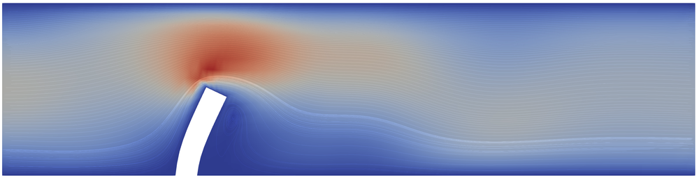
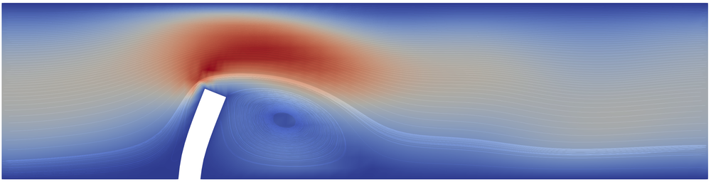
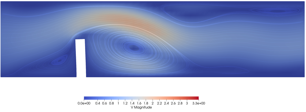
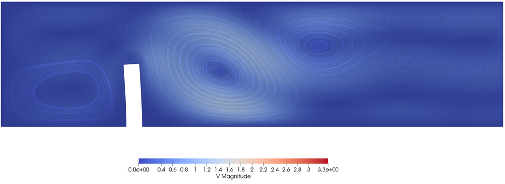
Figure 3: Solutions on the last 4 subintervals (from left to right), the deformation is magnified by a factor of 2.

(a) Coarse stepsize $K=0.01$

(b) Coarse stepsize $K=0.02$

(c) Coarse stepsize $K=0.05$

(d) Coarse stepsize $K=0.1$

Figure 4: Velocity error between sequential (computed with the fine stepsize $k$) and Parareal solution with different coarse step sizes calculated at the interval boundaries as the relative error in the Frobenius norm $\frac{\lVert v_{p}-v_{s}\rVert_{F}}{\lVert v_{s}\rVert_{F}}$. Where $v_{s}$ is the sequential solution and $v_{p}$ the Parareal solution. The dashed line is the difference between the sequential solution and a reference solution. All Parareal approximations below this line can be considered sufficiently accurate.

Figure 3 shows the solutions of the problems at time $t_{17}=6{.}8,\,t_{18}=7{.}2,\,t_{19}=7{.}6,\,t_{20}=8$. The dynamics of this problems is enforced by the oscillating right hand side that causes a periodic motion of the elastic obstacle.

In figure 4 we show the convergence behavior of the Parareal method for four choices of the large time step $K$. For each iteration $k$ of the Parareal method we plot the relative error between the Parareal approximation and a sequential solution (using the same small step size). The time interval is split into 20 subintervals and we clearly recognize that after the $k$-th iteration, the solution on the $k$-th interval does not get any better. All plots also include a dashed line (this is exactly the same line in every plot) which indicates the discretization error, e.g. the error between the sequential solution with stepsize $k$ and a refined reference solution. If the Parareal error is below this line, the Parareal approximation can be considered sufficiently accurate, e.g. considering $K=0.01$, two iterations $k=2$ already yield a Parareal approximation error that is smaller than the discretization error.

Furthermore, in figure 8 we give an overview of the speedup that is obtained in comparison to the sequential simulation. In this example the optimal choice would be $K=0{.}05$, stopping after 3 iterations such that the discretization error is dominant and resulting in a speedup of $3{.}45$.

That is below the theoretical value of $5{.}78$ estimated by from (12). The sub optimal performance is mostly due to the strong nonlinearity of the fluid-structure interaction problem. The nonlinear problems are approximated with a Newton’s method that benefits form small time-steps as they limit the role of the ALE map. Using coarser time steps for the prediction (that should theoretically improve the speedup) we require more Newton iterations such that the efficiency is reduced. The theoretical predictions can only be reached when the computational costs of each time step are exactly the same, which we cannot guarantee.

4.2 fsi-3 benchmark problem. A case where the algorithm fails

Figure 5: fsi-3 benchmark problem ([25]). Drag coefficient from the Parareal method after 2 iterations in comparison to the sequential solution at time step size $k=10^{-3}$. The coarse stepsize was chosen as $k=10^{-2}$. Oscillations occur after each Parareal update.

In the first experiments, we considered the fsi-3 benchmark problem as introduced by Hron and Turek [25]. In this case Parareal did not converge. Instead we observed pressure oscillations as shown in figure 5. One possible explanation for these instabilities that are also known from the simulation of incompressible flow problems on moving meshes [7] is the violation of the weak divergence freeness after the Parareal update $(\mathbf{u},\,\mathbf{v})_{m+k}^{\textrm{final}}=(\mathbf{u},\,\mathbf{v})_{m+k-1}^{C}+(\mathbf{u},\,\mathbf{v})_{m+k}^{F}-(\mathbf{u},\,\mathbf{v})_{m+k}^{C}$, as the nonlinear ALE formulation $(J\mathbf{F}^{-1}:\nabla\mathbf{v}^{T},\xi)_{{\cal F}}$ with separate updates in velocity and deformation does not conserve weak incompressibility and gives rise to pressure oscillations

$$i=1,2:\quad\big{(}\operatorname{det}(I+\nabla\mathbf{u}_{i})(I+\nabla\mathbf{u}_{i})^{-1}:\nabla\mathbf{v}^{T}_{i},\xi\big{)}_{{\cal F}}=0\\ \not\Rightarrow\quad\big{(}\operatorname{det}(I+\nabla(\mathbf{u}_{1}+\mathbf{u}_{2}))(I+\nabla(\mathbf{u}_{1}+\mathbf{u}_{2}))^{-1}:\nabla(\mathbf{v}_{1}+\mathbf{v}_{2})^{T},\xi\big{)}_{{\cal F}}=0.$$

Our approaches to avoid this problem, e. g. applying a Stokes projection to the initial solutions on the subintervals in every time steps, see [7], did not give remedy.

Another and more likely reason for the cause of these instabilities is the dependency of the damping properties of the shifted Crank-Nicolson time-stepping scheme on the time-step. Depending on the time step size, the problem shows a slightly shifted transient phase, e.g. the dominant oscillations in the drag coefficient are slightly and when the Parareal algorithm was applied these shifts caused instabilities. If the coarse time step was chosen so small that the dynamics did not differ in a destructive way, no speedup was achieved anymore. It could be worthwhile to test a damping $\theta=\frac{1}{2}+\alpha(k)k$ with a special choice of the parameter $\alpha(k)$, such that large time step and short time step have the same dissipation properties. In [38] Ruprecht suggests modifying the update in the parareal algorithm, such that information about the dissipation properties is taken into account.

4.3 3d example

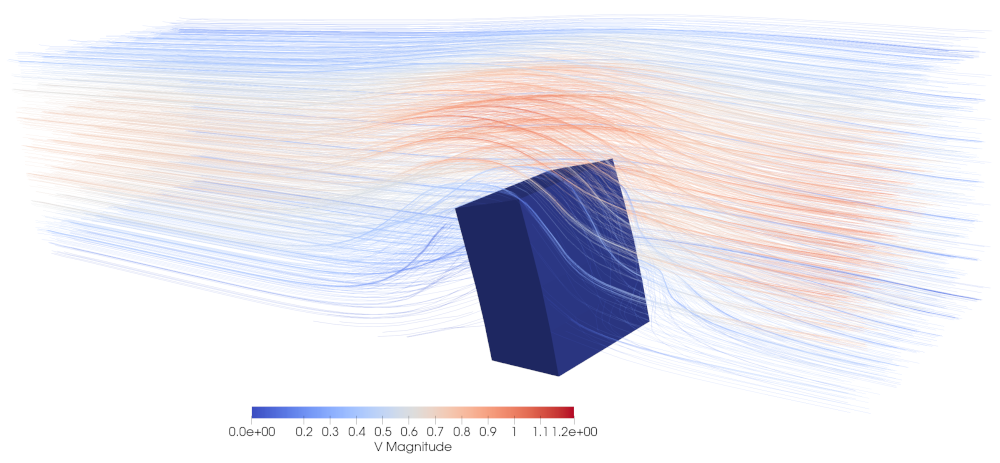
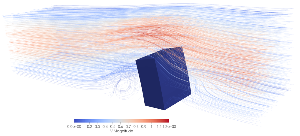
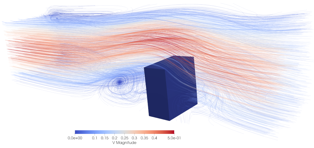
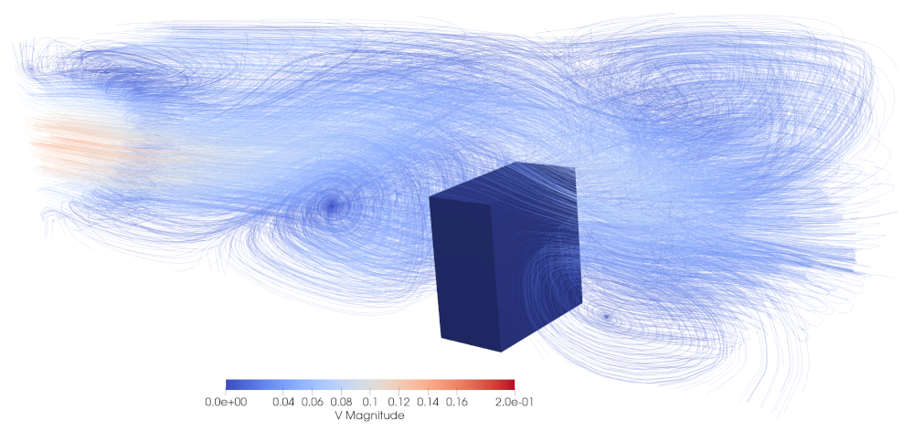
Figure 6: Solutions on the last 4 subintervals (from left to right), the deformation is magnified by a factor of 10.

(a) Coarse stepsize $K=0.01$

(b) Coarse stepsize $K=0.02$

(c) Coarse stepsize $K=0.05$

(d) Coarse stepsize $K=0.1$

Figure 7: Velocity error from the 3d case. We see the error between sequential (computed with the fine stepsize $k$) and Parareal solution with different coarse step sizes. They are calculated at the subinterval boundaries as the relative error in the Frobenius norm $\frac{\lVert v_{p}-v_{s}\rVert_{F}}{\lVert v_{s}\rVert_{F}}$. Where $v_{s}$ is the sequential solution and $v_{p}$ the Parareal solution. The bright grey line is the difference between the sequential solution and a reference solution.

Figure 6 shows the solution of the 3d problem $t_{17}=6{.}8,\,t_{18}=7{.}2,\,t_{19}=7{.}6,\,t_{20}=8$, analogous to the 2d case. In figure 7 we show the relative errors of the Parareal approximation in comparison to a sequential simulation for each iteration. Again, a dashed line represents the discretization error of the problem by comparison to a refined reference solution. We observe a similar behavior like in the 2d case: The Parareal error is quickly below the level of the discretization error and initial intervals do not benefit from further steps. However, figure 8 showing the speedups indicates a substantially reduced performance of the Parareal scheme when applied to this 3d test case. The main cause for this deterioration is the linearization of the problem: Newton’s method takes longer to converge for big timesteps and the corrections in the Parareal algorithm only seem to aggravate this problem. Although the instabilities noted in 4.2 could not be observed here, they start to rise: Larger timesteps influence the dynamics and if they get too large, the problems are not feasible in a stable manner anymore.

Due to these problems the Parareal algorithm is not guaranteed to give beneficial speedups in the 3d case. By choosing the timesteps carefully a speedup of $2{.}18$ can still be obtained.

(a) The 2d case

(b) The 3d case

Figure 8: Speedup of Parareal using 20 cores.

5 Conclusion

We applied the Parareal algorithm to fluid-structure interaction problems in 2d and 3d. Two cases were analyzed, in which speedup and convergence in very few iterations were achieved. We also saw notable limitations of the algorithm when applied to fluid-structure-interactions. One reason is the hyperbolic character of the solid problem that prevents the use of too coarse timesteps, as they can result in a different dynamics and an offset between predictor and corrector. The fsi-3 benchmark problem by Hron and Turek showed to be too challenging and it was not possible to pick discretization parameters that gave speedup and a stable solution at the same time.

Another issue is the severe nonlinearity of fluid-structure interactions. The design on nonlinear (and linear) solvers is already a challenge and coarse timesteps lead to an increased effort that limits the possible speedup.

The Parareal algorithm needs careful investigation of the problem before it can be successfully applied. Choosing the right time step sizes is crucial and even then it could still fail. If the problem is suitable on the other hand, it offers a simple way to speedup the solution.

References

• [1] E. Aubanel. Scheduling of tasks in the parareal algorithm. Parallel Computing, 37(3):172 – 182, 2011.
• [2] E. Aulisa, S. Bna, and G. Bornia. A monolithic ale newton-krylov solver with multigrid-richardson-schwarz preconditioning for incompressible fluid-structure interaction. Computers & Fluids, accepted 2018.
• [3] A.-M. Baudron, J.-J. Lautard, Y. Maday, M. Riahi, and J. Salomon. Parareal in time 3d numerical solver for the lwr benchmark neutron diffusion transient model. Journal of Computational Physics, 279:67–79, 2014.
• [4] R. Becker and M. Braack. Multigrid techniques for finite elements on locally refined meshes. Numerical Linear Algebra with Applications, 7:363–379, 2000. Special Issue.
• [5] R. Becker and M. Braack. A finite element pressure gradient stabilization for the Stokes equations based on local projections. Calcolo, 38(4):173–199, 2001.
• [6] R. Becker, M. Braack, D. Meidner, T. Richter, and B. Vexler. The finite element toolkit Gascoigne. http://www.gascoigne.uni-hd.de.
• [7] M. Besier and W. Wollner. On the pressure approximation in nonstationary incompressible flow simulations on dynamically varying spatial meshes. Int. J. Numer. Math. Fluids., 69:1054–1064, 2012.
• [8] A. Blouza, L. Boudin, and S.M. Kaber. Parallel in time algorithms with reduction methods for solving chemical kinetics. Communications in Applied Mathematics and Computational Science, 5(2):241–263, 2011.
• [9] E. Burman and P. Hansbo. Edge stabilization for the generalized Stokes problem: a continuous interior penalty method. Comput. Methods Appl. Mech. Engrg., 195(19):2393–2410, 2006.
• [10] P. Causin, J.F. Gereau, and F. Nobile. Added-mass effect in the design of partitioned algorithms for fluid-structure problems. Comput. Methods Appl. Mech. Engrg., 194:4506–4527, 2005.
• [11] P.G. Ciarlet. Finite Element Methods for Elliptic Problems. North-Holland, Amsterdam, 1978.
• [12] R. Croce, D. Ruprecht, and R. Krause. Parallel-in-space-and-time simulation of the three-dimensional, unsteady navier-stokes equations for incompressible flow. In Modeling, Simulation and Optimization of Complex Processes-HPSC 2012, pages 13–23. Springer, 2014.
• [13] J. Donea. An arbitrary lagrangian-eulerian finite element method for transient dynamic fluid-structure interactions. Comput. Methods Appl. Mech. Engrg., 33:689–723, 1982.
• [14] L. Failer and T. Richter. A parallel newton multigrid framework for monolithic fluid-structure interactions. submitted, 2019. XXXX - https://arxiv.org/.
• [15] M.A. Fernández and J.-F. Gerbeau. Algorithms for fluid-structure interaction problems. In L. Formaggia, A. Quarteroni, and A. Veneziani, editors, Cardiovascular Mathematics: Modeling and simulation of the circulatory system, volume 1 of MS & A, pages 307–346. Springer, 2009.
• [16] Paul F Fischer, Frédéric Hecht, and Yvon Maday. A parareal in time semi-implicit approximation of the navier-stokes equations. In Domain decomposition methods in science and engineering, pages 433–440. Springer, 2005.
• [17] S. Frei and T. Richter. A locally modified parametric finite element method for interface problems. SIAM J. Numer. Anal., 52(5):2315–2334, 2014.
• [18] M.J. Gander and S. Vandewalle. Analysis of the parareal time-parallel time-integration method. 29(2):556–578, 2007.
• [19] M.W. Gee, U. Küttler, and W.A. Wall. Truly monolithic algebraic multigrid for fluid-structure interaction. Int. J. Numer. Meth. Engrg., 85:987–1016, 2010.
• [20] T. Haut and B. Wingate. An asymptotic parallel-in-time method for highly oscillatory pdes. SIAM Journal on Scientific Computing, 36(2):A693–A713, 2014.
• [21] M. Heil, A.L. Hazel, and J. Boyle. Solvers for large-displacement fluid-structure interaction problems: Segregated vs. monolithic approaches. Computational Mechanics, 43:91–101, 2008.
• [22] J.G. Heywood, R. Rannacher, and S. Turek. Artificial boundaries and flux and pressure conditions for the incompressible Navier-Stokes equations. Int. J. Numer. Math. Fluids., 22:325–352, 1992.
• [23] C.W. Hirt, A.A. Amsden, and J.L. Cook. An Arbitrary Lagrangian-Eulerian computing method for all flow speeds. J. Comp. Phys., 14:227–469, 1974.
• [24] J. Hron and S. Turek. A monolithic FEM/Multigrid solver for an ALE formulation of fluid-structure interaction with applications in biomechanics. In H.-J. Bungartz and M. Schäfer, editors, Fluid-Structure Interaction: Modeling, Simulation, Optimization, Lecture Notes in Computational Science and Engineering, pages 146–170. Springer, 2006.
• [25] J. Hron and S. Turek. Proposal for numerical benchmarking of fluid-structure interaction between an elastic object and laminar incompressible flow. In H.-J. Bungartz and M. Schäfer, editors, Fluid-Structure Interaction: Modeling, Simulation, Optimization, Lecture Notes in Computational Science and Engineering, pages 371–385. Springer, 2006.
• [26] T.J.R. Hughes, W.K. Liu, and T.K. Zimmermann. Lagrangian-eulerian finite element formulations for incompressible viscous flows. Comput. Methods Appl. Mech. Engrg., 29:329–349, 1981.
• [27] A. Kreienbuehl, A. Naegel, D. Ruprecht, R. Speck, G. Wittum, and R. Krause. Numerical simulation of skin transport using parareal. Computing and visualization in science, 17(2):99–108, 2015.
• [28] U. Langer and H. Yang. Recent development of robust monolithic fluid-structure interaction solvers. In Fluid-Structure Interactions. Modeling, Adaptive Discretization and Solvers, volume 20 of Radon Series on Computational and Applied Mathematics. de Gruyter, 2017.
• [29] M. Lenoir. Optimal isoparametric finite elements and error estimates for domains involving curved boundaries. SIAM Journal on Numerical Analysis, 23(3):562–580, 1986.
• [30] J.-L. Lions, Y. Maday, and G. Turinici. Résolution d’edp par un schéma en temps. Comptes rendus de l’Académie des sciences I, Mathématique, 332(7):661–668, 2001.
• [31] M. Luskin and R. Rannacher. On the smoothing propoerty of the Crank-Nicholson scheme. Applicable Anal., 14:117–135, 1982.
• [32] M. Molnar. Stabilisierte Finite Elemente für Strömungsprobleme auf bewegten Gebieten. Master’s thesis, Universität Heidelberg, 2015.
• [33] R. Rannacher. Finite element solution of diffusion problems with irregular data. Numer. Math., 43:309–327, 1984.
• [34] T. Richter. A monolithic geometric multigrid solver for fluid-structure interactions in ALE formulation. Int. J. Numer. Meth. Engrg., 104(5):372–390, 2015.
• [35] T. Richter. Fluid-structure Interactions. Models, Analysis and Finite Elements, volume 118 of Lecture notes in computational science and engineering. Springer, 2017.
• [36] T. Richter and T. Wick. Finite elements for fluid-structure interaction in ALE and Fully Eulerian coordinates. Comput. Methods Appl. Mech. Engrg., 199(41-44):2633–2642, 2010.
• [37] T. Richter and T. Wick. On time discretizations of fluid-structure interactions. In T. Carraro, M. Geiger, S. Körkel, and R. Rannacher, editors, Multiple Shooting and Time Domain Decomposition Methods, volume 9 of Contributions in Mathematical and Computational Science, pages 377–400. Springer, 2015.
• [38] D. Ruprecht. Wave propagation characteristics of parareal. Computing and Visualization in Science, 19(1-2):1–17, 2018.
• [39] T. Richter S. Frei. Second order time-stepping for parabolic interface problems with moving interfaces. Mod\a’el. Math. Anal. Num\a’er., 2017. https://doi.org/10.1051/m2an/2016072.
• [40] D. Samaddar, D.E. Newman, and R. Sánchez. Parallelization in time of numerical simulations of fully-developed plasma turbulence using the parareal algorithm. Journal of Computational Physics, 229(18):6558–6573, 2010.
• [41] S. Turek, J. Hron, M. Madlik, M. Razzaq, H. Wobker, and J. Acker. Numerical simulation and benchmarking of a monolithic multigrid solver for fluid–structure interaction problems with application to hemodynamics. Technical report, Fakultät für Mathematik, TU Dortmund, February 2010. Ergebnisberichte des Instituts für Angewandte Mathematik, Nummer 403.
• [42] S. Turek, L. Rivkind, J. Hron, and R. Glowinski. Numerical study of a modified time–stepping theta–scheme for incompressible flow simulations. Journal of Scientific Computing, 28(2–3):533–547, 2006.