Geometric Crossing-Minimization – A Scalable Randomized Approach

Abstract

We consider the minimization of edge-crossings in geometric drawings of graphs $G=(V,E)$, i.e., in drawings where each edge is depicted as a line segment. The respective decision problem is $\mathcal{NP}$-hard [5]. Crossing-minimization, in general, is a popular theoretical research topic; see Vrt’o [26]. In contrast to theory and the topological setting, the geometric setting did not receive a lot of attention in practice. Prior work [21] is limited to the crossing-minimization in geometric graphs with less than $200$ edges. The described heuristics base on the primitive operation of moving a single vertex $v$ to its crossing-minimal position, i.e., the position in $\mathbb{R}^{2}$ that minimizes the number of crossings on edges incident to $v$.

In this paper, we introduce a technique to speed-up the computation by a factor of $20$. This is necessary but not sufficient to cope with graphs with a few thousand edges. In order to handle larger graphs, we drop the condition that each vertex $v$ has to be moved to its crossing-minimal position and compute a position that is only optimal with respect to a small random subset of the edges. In our theoretical contribution, we consider drawings that contain for each edge $uv\in E$ and each position $p\in\mathbb{R}^{2}$ for $v$ $o(|E|)$ crossings. In this case, we prove that with a random subset of the edges of size $\Theta(k\log k)$ the co-crossing number of a degree-$k$ vertex $v$, i.e., the number of edge pairs $uv\in E,e\in E$ that do not cross, can be approximated by an arbitrary but fixed factor $\delta$ with high probability. In our experimental evaluation, we show that the randomized approach reduces the number of crossings in graphs with up to $13\,000$ edges considerably. The evaluation suggests that depending on the degree-distribution different strategies result in the fewest number of crossings.

1 Introduction

The minimization of crossings in geometric drawings of graphs is a fundamental graph drawing problem. In general the problem is $\mathcal{NP}$-hard [13, 5] and has been studied from numerous theoretical perspectives; see Vrt’o [26]. Until recently only the topological setting, where edges are drawn as topological curves, has been considered in practice [14, 6, 8]. In our previous paper [21] we describe geometric heuristics that compute straight-line drawings of graphs with significantly fewer crossings compared to common energy-based layouts. One of the heuristics is the vertex-movement approach that iteratively moves a single vertex $v$ to its crossing-minimal position, i.e., a position $p^{\star}$ so that crossings of edges incident to $v$ are minimized. Unfortunately, the worst-case running time to compute this position is super-quadratic in the size of the graph as the following theorem states.

Theorem 1 (Radermacher et al. [21]).

The crossing-minimal position of a degree-$k$ vertex $v$ with respect to a straight-line drawing $\Gamma$ of a graph $G=(V,E)$ can be computed in $O\left((kn+m)^{2}\log\left(kn+m\right)\right)$ time, where $n=|V|,m=|E|$.

This is not only a theoretical upper bound on the running time but is also a limitation that has been observed in practice. The implementation we used previously requires considerable time to compute drawings with few crossings. For this reason we were only able evaluate our approach on graphs with at most $200$ edges. For example, on a class of graphs that have $64$ vertices and $196$ edges our implementation already required on average about 35 seconds to compute a drawing with few crossings.

Energy-based methods are common and well engineered tools to draw graphs [16]. For example, the aim of Stress Majorization (or simply Stress) is to compute a drawing such that the Euclidean distance of each two vertices corresponds to their graph-theoretical distance [12]. The algorithm has been engineered to handle graphs with up to $10^{6}$ vertices and $3\cdot 10^{6}$ edges [19]. Kobourov [16] claimed that Stress tends to minimize the number of crossings. In our previous experimental evaluation [21] we demonstrated that the statement is not true for a varied set of graph classes.

Fabila-Monroy and López [11] introduced a randomized algorithm to compute a drawing of $K_{n}$ with a small number of crossings. Many best known upper bounds on the rectilinear crossing number of $K_{n}$, for $44\leq k\leq 99$, are due to this approach [1]. The algorithm iteratively updates a set $P$ of $n$ points, by replacing a random point $p\in P$ by a random point $q$ that is close to $p$, if $q$ improves the number of crossings. Since the number of crossings of $K_{n}$ is in $\Theta(n^{4})$, the bottleneck of their approach is the running time for counting the number of crossings induced by $P$. A similar randomized approach has been used to maximize the smallest crossing angle in a straight-line drawing [3, 10]. The approach iteratively moves vertices to the best position within a random point set.

Contribution.

The main contribution of this paper is to engineer the vertex-movement approach for the minimization of crossings in geometric drawings described in [21] to be applicable on graphs with a few thousands vertices and edges.

1. In Section 3 we introduce so-called bloated duals of line arrangements, a combinatorial technique to construct a dual representation of general line arrangements. In our application this results in an overall speed-up of about a factor of $20$ in comparison to the recent implementation. This speed-up is necessary but not sufficient to handle graphs with a few thousands vertices and edges.

2. In Section 4 we demonstrate that taking a small random subset of the edges is sufficient to compute drawings with few crossings. Moreover, in Section 4.1 we prove that under certain conditions the randomized approach is an approximation of the co-crossing number of a vertex, with high probability.

3. Based on the insights of the evaluation in Section 4.2, we introduce a weighted sampling approach. A comparison to a restrictive approach of sampling points suggests that the degree-distribution of the graph is a good indicator to decide which approach results in fewer crossings.

4. Overall, our experimental evaluation shows that we are now able to handle graphs with $12\,000$ edges, which are $60$ times more than the graphs that have been considered in the evaluation in [21].

2 Preliminaries

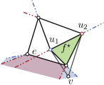
Figure 1: The black, blue and red segments show the arrangement $\mathcal{A}(\Gamma,v)$ of the black drawing $\Gamma$. The blue and red region show the complement of the visibility regions of $u_{1}$ and $u_{2}$, respectively, and the edge $e$. The green region is crossing minimal.

We repeat some notation from [21]. Let $\Gamma$ be a straight-line drawing of a $G=(V,E)$. Denote by $N(v)\subseteq V$ the set of neighbors of $v$ and by $E(v)\subseteq E$ the set of edges incident to $v$. For a vertex $v\in V$, denote by $\Gamma[v\mapsto p]$ the drawing that is obtained from $\Gamma$ by moving the vertex $v$ to the point $p$. We denote the number of crossings in a drawing $\Gamma$ by $\operatorname{{\mathrm{cr}}}(\Gamma)$, the number of crossings on edges incident to $v$ by $\operatorname{{\mathrm{cr}}}(\Gamma,v)$, and we refer with $\operatorname{{\mathrm{cr}}}(\Gamma,e,f)$ to the number of crossings on two edges $e$ and $f$ in $\Gamma$, i.e., $\operatorname{{\mathrm{cr}}}(\Gamma,e,f)\in\{0,1\}$ if $e\not=f$. For a point $u$ and a segment $e$, denote by $\operatorname{\mathcal{VR}}(u,e)$ the visibility region of $u$ and $e$, i.e., the set of points $p\in\mathbb{R}^{2}$ such that the segment $up$ and $e$ do not intersect. Moreover, let $\operatorname{\mathcal{BD}}(u,e)$ be the boundary of $\operatorname{\mathcal{VR}}(u,e)$. Let $\mathcal{A}(\Gamma,v)$ be the arrangement over all boundaries $\operatorname{\mathcal{BD}}(u,e)$ for each neighbor $u\in N(v)$ of $v$ and each edge $e\in E\setminus E(u)$; see Figure 1. The arrangement has the property that two points $p$ and $q$ in a common cell of $\mathcal{A}(\Gamma,v)$ induce the same number of crossings for $v$, i.e., $\operatorname{{\mathrm{cr}}}(\Gamma[v\mapsto p],v)=\operatorname{{\mathrm{cr}}}(\Gamma[v\mapsto q],v)$ [21]. Thus, the computation of a crossing minimal position $p^{\star}$ reduces to finding a crossing-minimal region $f^{\star}$ in $\mathcal{A}(\Gamma,v)$.

For our experiments, we used two different compute servers. Both systems ran with an openSUSE Leap 15.0 operating system. All algorithms were compiled with g++ version 7.3.1 with optimization mode -O3. System 1 was used for running time experiments, i.e., for the experiments evaluated in Section 3.1 and in Section 4.2. System 2 is used for the experiments evaluated in Section 4.3.

System 1

Intel Xeon(tm) E5-1630v3 processor clocked at 3.7 GHz, 128 GB RAM.

System 2

Two Intel Xeon(tm) E5-2670 CPU processors clocked at 2.6 GHz, 64 GB RAM.

3 Efficient Implementation of the Crossing-Minimal Position

The vertex-movement approach iteratively moves a single vertex to its crossing-minimal position. The running time of the overall algorithm crucially depends on an efficient computation of this operation. Therefore the aim of this section is to provide an efficient implementation of the crossing-minimal position of a vertex. Our previous implementation [21] heavily relies on CGAL [24], which follows an exact computations paradigm and uses exact number types to, e.g., represent coordinates and intermediate results. This helps to ensure correctness but considerably increases the running time of the algorithms. We introduce an approach to compute the crossing-minimal position that drastically reduces the usage of exact computations.

Computing a crossing-minimal position of a vertex $v$ is equivalent to computing a crossing-minimal region $f^{\star}$ in the arrangement $\mathcal{A}(\Gamma,v)$. The region $f^{\star}$ of a vertex $v$ can be computed by a breadth-first search in the dual graph $\mathcal{A}(\Gamma,v)^{\star}$. Thus, the time-consuming steps to compute $f^{\star}$ are to construct the arrangement $\mathcal{A}(\Gamma,v)$ and then to build the dual $\mathcal{A}(\Gamma,v)^{\star}$. Instead of computing the dual $\mathcal{A}(\Gamma,v)^{\star}$ we construct a so-called bloated dual $\mathcal{A}(\Gamma,v)^{+}$. The advantage of this approach is that it suffices to compute the set of intersecting segments in $\mathcal{A}(\Gamma,v)$ to construct $\mathcal{A}(\Gamma,v)^{+}$ and it is not necessary to compute the arrangement $\mathcal{A}(\Gamma,v)$ itself, i.e., the exact coordinates of each intersection.

(a)

(b)

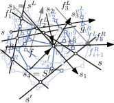
(c)

Figure 2: (a) Bloated dual $\mathcal{A}^{+}$ (blue) of an arrangement $\mathcal{A}$ (black). Inserting edges dual to a segment $s$ (b) and within a face (c).

Let $S$ be a set of line segments and let $\mathcal{A}$ be the arrangement of $S$. A bloated dual of $\mathcal{A}$ is a graph $\mathcal{A}^{+}$ that has the following properties (compare Figure 2(a)):

1. each edge $e$ incident to a face $f$ corresponds to a vertex $v_{e}^{f}$ in $\mathcal{A}^{+}$,

2. if two distinct segments $s,s^{\prime}\in S$ of $f$ have a common intersection on the boundary of $f$, then $v_{s}^{f}v_{s^{\prime}}^{f}\in E(\mathcal{A}^{+})$, and

3. for two distinct faces $f,g$ sharing a common segment $s$, there is an edge $v_{s}^{f}v_{s}^{g}\in E(\mathcal{A}^{+})$.

Note that given a crossing-minimal face and $v^{f}_{s_{0}}$, the geometric representation of $f$ has to be computed in order to compute a crossing-minimal position $p\in f$. Further a vertex $v^{f}_{s_{0}}$ belongs to a cycle $v^{f}_{s_{0}},v^{f}_{s_{1}},\dots v^{f}_{s_{k}}$. Then, the geometric representation of the boundary of $f$ can be computed by intersecting the segments $s_{i}$ and $s_{i+1}$, where we set $k+1=0$. In the following, we will show that it is sufficient to know the order in which the segments in $S$ intersect to construct the bloated dual. Thus, exact number types only have to be used to determine the order of two segments whose intersections with a third segment $s$ have a small distance on $s$.

We construct the bloated dual of $\mathcal{A}$ in two steps. First, we insert all vertices $v_{s}^{f},v^{g}_{s}$ and the corresponding edge $v_{s}^{f}v_{s}^{g}$. In the second step, we insert the remaining edges $v_{s}^{f}v_{s^{\prime}}^{f}$ within a face $f$. For a compact description we assume that no intersection point of two segments is an endpoint of a segment. We define the source of $s$ and target of $s$ to be the lexicographically smallest and largest point on $s$, respectively. We direct each segment $s$ from its source to its target.

Let $p_{1},p_{2},\dots,p_{l}$ be the intersection points on a segment $s$ in lexicographical order. These intersection points correspond to a set of left faces $f^{L}_{1},f^{L}_{2},\dots,f^{L}_{l+1}$ and to a set of right faces $f^{R}_{1},f^{R}_{2},\dots,f^{R}_{l+1}$, such that $f^{L}_{i}$ and $f^{R}_{i}$ share parts of their boundary; see Figure 2(b). Thus, we can associate a set of vertices $v^{L}_{i},v^{R}_{i},2\leq i\leq l+1$, with $s$, and add the edges $v^{L}_{i}v^{R}_{i}$ to $\mathcal{A}^{+}$. Note that only the order and not the actual coordinates of the points $p_{1},\dots,p_{l}$ has to be known to insert the edges. Thus, given the set of segments that intersect $s$, an exact number type is only necessary to determine the order of two segments $s_{i}$ and $s_{j}$ whose intersection points $p_{i}$ and $p_{j}$ on $s$ have a small distance.

We now add the remaining edges within a face $f$. Let $S^{\prime}=\{s_{1},\dots,s_{k}\}\subseteq S$ be the set of segments that intersect $s$ in $p_{i}$; see Figure 2(c). The two segments $s^{L},s^{R}\in S^{\prime}$ that lie on the boundary of $f^{L}_{i}$ and $f^{R}_{i}$ can be determined as follows. To find the segment $s^{L}$, we distinguish two cases. First, assume that there exists a segment $s^{\prime}\in S^{\prime}$ whose source is left of $s$. Observe that if there is a segment $s^{\prime\prime}$ whose target is left of $s$, the segment $s^{\prime\prime}$ cannot be the segment $s^{L}$. Thus, we assume without loss of generality that all sources of segments in $S^{i}_{s}$ are left of $s$. Then a segment $s^{\prime}\in S^{\prime}$ is the segment $s^{L}$ if and only if the segment $s^{\prime}$ and each segment $s^{\prime\prime}\in S^{\prime}\setminus\{s^{\prime}\}$ form a right turn. Now consider the case that there is no segment whose source is left of $s$. Then a segment $s^{\prime}$ is $s^{L}$ if and only if the segment $s^{\prime}$ and each segment $s^{\prime\prime}\in S^{\prime}\setminus\{s^{\prime}\}$ form a left turn. The segment $s^{R}$ can be determined analogously.

Implementation Details.

We give some implementation details which allow us to efficiently implement the construction of the bloated dual. We use the index of a vertex to decide whether it is left or right of $s$, i.e., vertices with an odd index are left of $s$ and vertices with an even index are right of $s$. The fact that each vertex of $\mathcal{A}^{+}$ has degree at most 3 allows us to represent $\mathcal{A}^{+}$ as a single array $B$ of size $3n$, where $n$ is the number of vertices of $\mathcal{A}^{+}$. The vertices incident to a vertex $v_{i}$ occupy the cells $B[3i],B[3i+1]$ and $B[3i+2]$. Moreover, each pair of segments in $S$ can be handled independently to construct the bloated dual. This enables a parallelization over the segments in $S$.

3.1 Evaluation of the Running Time

(a)

(b)

(c)

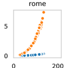
(d)

Figure 3: Comparing the running time of two approaches (orange Precise, blue Bd) to compute the crossing minimal region. Each point corresponds to a graph $G$. The $x$-axis shows the number of edges of $G$. The $y$-axis depicts the running time in seconds to compute the crossing minimal regions for all vertices of $G$.

In this section, we compare the running time of the two approaches to compute the crossing-minimal region of a vertex. We refer with Precise to the approach that uses CGAL to compute the crossing minimal region and with Bd to the approach based on the bloated dual. In order to compute all intersecting segments, we use a naive implementation of a sweep-line algorithm [4]. In this approach all segments within a specific interval are pairwise checked for an intersection. This has the advantage that the computation is independent of the coordinates of the intersection.

The experimental setup is as follows. Given a drawing $\Gamma$ of a graph $G$, we are interested in the running time of moving all vertices of a graph to their crossing-minimal positions. Therefore, we measure the running time of computing the crossing-minimal regions of all vertices. In order to guarantee the comparability of the two approaches, we use the same vertex order and only compute the crossing-minimal region but do not update the positions of the vertices. We use the same set of benchmark graphs used in [21]: North, Rome¹, graphs that have Community structure, and Triangulations on 64 vertices with an additional $10$ random edges. For each graph class, 100 graphs were selected uniformly at random. We use the implementation of Stress [12] provided by Ogdf [7] (snapshot 2017-07-23) to compute an initial layout of the graphs.

The plots in Figure 3 shows the results of the experiments. Each point in the plot corresponds to the running time of computing all crossing-minimal region of a single graph. The plot shows that the Bd implementation is considerably faster than the Precise implementation. For each graph class, we achieve on average a speed-up of at least $20$. The minimum speed-up on the North graphs is $8$. For each graph class, the speed-up is at least 18 for at least 75 out of 100 instances.

4 Random Sampling

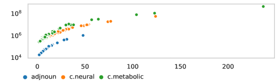
Figure 4: The $x$-axis shows the vertex-degree and the $y$-axis the number of intersecting edges in the arrangement $\mathcal{A}(\Gamma,v)$. The $y$-axis is in $\log$-scale.

The worst-case running time of computing the crossing-minimal region of a vertex $v$ is super-quadratic in the size of the graph, see Theorem 1. Figure 4 shows the number of intersecting segment in the arrangement $\mathcal{A}(\Gamma,v)$ compared to the vertex-degree of $v$, for vertices of three selected graphs with at most 2 133 edges, compare Table 1. For these graphs the arrangement already contains up to $440\,685\,519$ intersecting segments. Indeed, we were not able to compute the number of intersections for all vertices of the graph c.metabolic, since the algorithm ran out of memory first. Due to the high number of intersections in graphs with a high number of edges or a large maximum vertex-degree, it is for these graphs infeasible to compute a crossing-minimal position of a vertex. This motivates the following question: Is a small subgraph of $G$ sufficient to considerably reduce the number of crossings in a given drawing?

To address this question, we follow the vertex-movement approach. Let $\Gamma_{0}$ be a drawing of $G$ and let $v_{1},v_{2},\dots,v_{n}$ be an ordered set of the vertices $V$ of $G$. For each vertex $v_{i}$ we obtain a new drawing $\Gamma_{i}$ from the drawing $\Gamma_{i-1}$ by moving $v_{i}$ to a new position $p^{\star}_{i}$. To compute the new position we consider a primal sampling approach, i.e., a sampling of points in the solution space $\mathbb{R}^{2}$, and a dual sampling approach, i.e., a sampling of edges that induce constraints to the solution space.

More formally, we consider the following approach to compute a new position of a single vertex $v_{i}$. Let $S_{i}\subset E$ be a uniform random subset of the edges of $G$ and let $V(S_{i})\subset V$ be the vertices that are incident to an edge in $S_{i}$. The graph $G|_{S_{i}}=(V(S_{i})\cup N(v_{i})\cup\{v_{i}\},S_{i}\cup E(v_{i}))$ induces a drawing $\Gamma|_{S_{i}}$ in $\Gamma_{i-1}$. Let $R_{i}$ be the crossing-minimal region of $v_{i}$ with respect to the drawing $\Gamma|_{S_{i}}$. Recall that for $S_{i}=E$ the region $R_{i}$ has the property that $\operatorname{{\mathrm{cr}}}(\Gamma|_{S_{i}}[v_{i}\mapsto p],v_{i})=\operatorname{{\mathrm{cr}}}(\Gamma|_{S_{i}}[v_{i}\mapsto q],v_{i})$ for any two points $p,q\in R_{i}$, compare Section 2. If $S_{i}$ is a strict subset of $E$, then $R_{i}$ does not necessarily have this property anymore. For this reason, let $P_{i}\subset R_{i}$ be a set of uniform random points and let $p_{i}^{\star}\in P_{i}\cup\{p_{i}^{\prime}\}$ be the point that minimizes $\operatorname{{\mathrm{cr}}}(\Gamma[v\mapsto p_{i}^{\star}],v_{i})$, where $p_{i}^{\prime}$ is the position of $v_{i}$ in $\Gamma_{i-1}$.

This remainder of this section is organized as follows. First, we analyze the dual sampling from a theoretical perspective (Section 4.1), followed by an experimental evaluation that compares the primal to the dual sampling (Section 4.2). Finally, based on the insights from this evaluation, we introduce in Section 4.3 a weighted sampling approach that is less restrictive than the dual sampling.

4.1 Approximating the Co-Crossing Number of a Vertex

In this section we study the dual sampling approach, i.e., the sampling of edges, with tools introduced in the context of the theory of VC-dimension. A thorough introduction into the theory of VC-dimension can be found in Matoušek’s Lectures on Discrete Geometry [18]. For a fixed vertex $v$, a drawing $\Gamma$ is $\varepsilon$-well behaved if for each point $p\in\mathbb{R}^{2}$ and each vertex $u\in N(v)$, the edge $uv$ crosses at most $(1-\varepsilon)|E|$ edges in the drawing $\Gamma[v\mapsto p]$. The co-crossing number $\operatorname{{\mathrm{co-cr}}}(\Gamma,v)$ of a vertex $v$ is the number of edge pairs $e\in E$ and $uv\in E$ that do not cross. We show that given an $\varepsilon$-well-behaved drawing $\Gamma$ of a graph $G=(V,E)$ and a degree-$k$ vertex $v$, a random sample $S\subset E$ of size $\Theta(k\log k)$ enables us to compute a position $q^{\star}$ whose co-crossing number is a $(1-\delta)$-approximation of the co-crossing number of a vertex $v$. Note that we are not able to guarantee that a large co-crossing number of a vertex $v$ implies a small crossing number of $v$. On the other hand, the co-crossing number is of interest for a variety of (sparse) graph. For example, drawings that contain many triangles are $\varepsilon$-well-behaved, since every line intersects at most two segments of a triangle.

A set system is a tuple $(X,\mathcal{F})$ with a base set $X$ and $\mathcal{F}\subseteq 2^{X}$. In the following, we assume $X$ to be finite. For some parameters $\varepsilon,\delta\in(0,1]$, a set $S\subseteq X$ is a relative $(\varepsilon,\delta)$-approximation for the set system $(X,\mathcal{F})$ if for each $R\in\mathcal{F}$ the following inequality holds.

$$\left|{\frac{\left|{S\cap R}\right|}{\left|{S}\right|}-\frac{\left|{R}\right|}{\left|{X}\right|}}\right|\leq\delta\max\{\frac{\left|{R}\right|}{\left|{X}\right|},\varepsilon\}$$ (1)

The proof of the following proposition and of proofs of statements that are marked with ($\star$) can be found in Appendix C.

Proposition 4.2 ($\star$).

For $\varepsilon,\delta\in(0,1]$, let $S$ be an $(\varepsilon,\delta)$-approximation of the set system $(X,\mathcal{F})$. If every $R\in\mathcal{F}$ has size at least $\varepsilon|X|$ then Equation 1 can be rewritten as follows:

$$(1-\delta)\left|{R}\right|\leq|X|\frac{\left|{S\cap R}\right|}{\left|{S}\right|}\leq(1+\delta)\left|{R}\right|.$$

Let $\mathcal{F}|_{A}=\{R\cap A\mid R\in\mathcal{F}\}$ be the restriction of $\mathcal{F}$ to a set $A\subseteq X$. A set $A\subseteq X$ is shattered by $\mathcal{F}$ if every subset of $A$ can be obtained by an intersection of $A$ with a set $R\in\mathcal{F}$, i.e., $\mathcal{F}|_{A}=2^{A}$. The VC-dimension of a set system $(X,\mathcal{F})$ is the size of the largest subset $A\subseteq X$ such that $A$ is shattered by $\mathcal{F}$ [25].

Theorem 4.3 (Har-Peled and Sharir [15], Li et al. [17]).

Let $(X,\mathcal{F})$ be a finite set system with VC-dimension $d$, and let $\delta,\varepsilon,\gamma\in(0,1]$. A uniform random sample $S\subseteq X$ of size

$$\Theta\left(\frac{d\cdot\log\varepsilon^{-1}+\log\gamma^{-1}}{\varepsilon\delta^{2}}\right)$$

is a relative $(\varepsilon,\delta)$-approximation for $(X,\mathcal{F})$ with probability $(1-\gamma)$.

For a vertex $u\in N(v)$, let ${\overline{{\mathbb{E}_{uv}(\Gamma)}}}=\{e\in E\mid\operatorname{{\mathrm{cr}}}(\Gamma,e,uv)=0\}$ denote the set of edges that are not crossed by the edge $uv$ in $\Gamma$. Then we have $\operatorname{{\mathrm{co-cr}}}(\Gamma,v)=\sum_{u\in N(v)}\left|{{\overline{{\mathbb{E}_{uv}(\Gamma)}}}}\right|$. Moreover, let ${\overline{{\mathbb{E}_{uv}(p)}}}={\overline{{\mathbb{E}_{uv}(\Gamma[v\mapsto p])}}}$. Then the set $\overline{\mathcal{F}_{uv}}=\bigcup_{p\in\mathbb{R}^{2}}\left\{{\overline{{\mathbb{E}_{uv}(p)}}}\right\}$ contains for each drawing $\Gamma[v\mapsto p]$ the set of edges that are not crossed by the edges $uv$, i.e, ${\overline{{\mathbb{E}_{uv}(p)}}}$. In particular $(E,\overline{\mathcal{F}_{uv}})$ is a set system and we will prove that it has bounded VC-dimension. This allows us to approximate the number of edges that are not crossed by the edge $uv$. We facilitate this to approximate the co-crossing number of a vertex for $\varepsilon$-well behaved drawings.

Lemma 4.4.

The VC-dimension of the set system $(E,\overline{\mathcal{F}_{uv}})$ is at most 8.

Proof 4.5.

Recall that that vertex $u$ has a fixed position. Let $\operatorname{\mathcal{BD}}(u,e)$ be the boundary of the visibility region of $u$ and the edge $e\in E$. Let $\mathcal{A}$ denote the arrangement of all boundaries $\operatorname{\mathcal{BD}}(u,e),e\in E$. Let $F$ be the set of faces in $\mathcal{A}$. Note that by Lemma 3.1 in [21] for every two points $p,q\in f$ the sets $E_{p}$ and $E_{q}$ of edges that have a non-empty intersection with the edge $uv$ when $v$ is moved to $p$ and $q$, respectively, coincide. Hence, the set $E_{f}\subseteq E$ of edges that cross the edge $uv$, in the drawing obtained from $\Gamma$ where $v$ is moved to an arbitrary position in $f$, is well defined. Thus, the number of faces $|F|$ is an upper bound for $\left|{\overline{\mathcal{F}_{uv}|_{A}}}\right|$ for every $A\subset E$. Note that there may be subsets of $E$ that are represented by more than one face. Moreover, observe that the visibility region $\operatorname{\mathcal{VR}}(u,e)$ is the intersection of three half-planes. Let $l^{1}_{e},l^{2}_{e},l^{3}_{e}$ be the supporting lines of these half-planes and let $\mathcal{A}^{\prime}$ be the arrangement of lines $l^{i}_{e},e\in E$. Hence, the number of faces in the arrangement $\mathcal{A}^{\prime}$ of $3m$ lines is an upper bound for $|F|$, with $m=|E|$. The number of faces $|F^{\prime}|$ of $\mathcal{A}^{\prime}$ is bounded by $f(m):=3m(3m-1)/2+1$ [20]. Thus, it is not possible to shatter a set $A\subset E$ if the number of faces $|F^{\prime}|$ is smaller than the number of subsets of $A$. The largest number for which the equality $2^{m}\leq f(m)$ holds is between $8$ and $9$. Since $2^{m}$ grows faster than $f(m)$, the largest set that can possibly be shattered has size at most $8$.

Due to Proposition 4.2 and Theorem 4.3 a relative $(\varepsilon,\delta)$-approximation $S_{u}$ of $(E,\overline{\mathcal{F}_{uv}})$ allows us to approximate the number of edges that are not crossed by the edge $uv$. In the following we show that we can approximate the co-crossing number of a vertex $v$ in any drawing $\Gamma[v\mapsto p]$ if we are given a relative $(\varepsilon,\delta)$-approximation $S_{u}$ for each vertex $u$ that is adjacent to $v$. The number $|{\overline{{\mathbb{E}_{uv}(p)}}}\cap S_{u}|/|S_{u}|$ corresponds to the relative number of edges in $S_{u}$ that are not crossed by the edge $uv$. Hence, the function $\lambda(p)=|E|\sum_{u\in U}{\lvert{{\overline{{\mathbb{E}_{uv}(p)}}}\cap S_{u}}\rvert}/{\lvert{S_{u}}\rvert}$ can be seen as an estimation of $\operatorname{{\mathrm{co-cr}}}(p)=\operatorname{{\mathrm{co-cr}}}(\Gamma[v\mapsto p],v)$.

Lemma 4.6 ($\star$).

Let $\varepsilon,\delta\in(0,1]$ be two parameters and let $\Gamma$ be an $\varepsilon$-well behaved drawing of $G$. For every $u\in N(v)$, let $S_{u}$ be a relative $(\varepsilon,\delta)$-approximation of the set system $(E,\overline{\mathcal{F}_{uv}})$. Then $(1-\delta)\operatorname{{\mathrm{co-cr}}}(p)\leq\lambda(p)\leq(1+\delta)\operatorname{{\mathrm{co-cr}}}(p)$ holds for all $p\in\mathbb{R}^{2}$.

Assume that $\varepsilon,\delta,\gamma\in(0,1)$ are constants. Lemma 4.6 shows that $k$ independent samples $S_{u}$ of constant size approximate the co-crossing number of $v$. By slightly increasing the number of samples, we can use a single set $S$ for all neighbors $u$. This reduces the running time from $O(k^{3}\log k)$ to $O(k^{2}\log^{3}k)$.

Lemma 4.7 ($\star$).

Let $v$ be a degree-$k$ vertex and let $\varepsilon,\delta,\gamma\in(0,1]$ with $\gamma\leq 1/k$. A uniformly random sample $S\subseteq E$ of size $\Theta\left((\log\varepsilon^{-1}+\log\gamma^{-1})/(\varepsilon\delta^{2})\right)$ is a relative $(\varepsilon,\delta)$-approximation the set system $(E,\overline{\mathcal{F}_{uv}})$ with probability $1-k\gamma$, for each $uv\in E$.

With Lemma 4.6 and Lemma 4.7 at hand, we have all the necessary tools to prove the main theorem.

Theorem 4.8.

Let $\varepsilon,\delta,\gamma\in(0,1]$ be three constants and let $G=(V,E)$ be a graph with a $\varepsilon$-well behaved drawing $\Gamma$ and let $v\in V$ be a degree-$k$ vertex. Let $p^{\star}$ be the position that maximizes $\operatorname{{\mathrm{co-cr}}}(\Gamma[v\mapsto p^{\star}],v)$. A $(1-\delta)$-approximation of $\operatorname{{\mathrm{co-cr}}}(\Gamma[v\mapsto p^{\star}])$ can be computed in $O\left(k^{2}\log^{3}k\right)$ time with probability $1-\gamma$.

Proof 4.9.

Let $\gamma^{\prime}=\gamma\cdot k^{-1}$ and $\delta^{\prime}=\delta/2$. Let $S\subseteq E$ be a uniformly random sample of size $\Theta\left((\log\varepsilon^{-1}+\log\gamma^{\prime-1})/(\varepsilon\delta^{\prime 2})\right)$. According to Lemma 4.7, for each $uv\in E$, the sample $S$ is a $(\varepsilon,\delta^{\prime})$-approximation of the $(E,\overline{\mathcal{F}_{uv}})$ with probability $1-k\gamma^{\prime}=1-\gamma$.

According to Lemma 4.6 the expected number of crossing-free edges $\lambda(p)$ is a $(1-\delta)$-approximation of $\operatorname{{\mathrm{co-cr}}}(p)$, i.e., $(1+\delta^{\prime})\operatorname{{\mathrm{co-cr}}}(q)\geq\lambda(q)\geq(1-\delta^{\prime})\operatorname{{\mathrm{co-cr}}}(q)$. Let $p^{\star}$ be the position that maximizes $\operatorname{{\mathrm{co-cr}}}(p)$ and let $q^{\star}$ be the position that maximizes $\lambda(q)$. Hence, we have $\lambda(q^{\star})\geq\lambda(p^{\star})$. Observe that over $\delta^{\prime}>0$ the inequality $(1-\delta^{\prime})/(1+\delta^{\prime})\geq 1-2\delta^{\prime}$ holds. We use this to prove that $\operatorname{{\mathrm{co-cr}}}(q^{\star})\geq(1-2\delta^{\prime})\operatorname{{\mathrm{co-cr}}}(p^{\star})$.

$$\operatorname{{\mathrm{co-cr}}}(q^{\star})\geq\frac{1}{(1+\delta^{\prime})}\lambda(q^{\star})\geq\frac{1}{(1+\delta^{\prime})}\lambda(p^{\star})\geq\frac{1-\delta^{\prime}}{1+\delta^{\prime}}\operatorname{{\mathrm{co-cr}}}(p^{\star})\geq(1-2\delta^{\prime})\operatorname{{\mathrm{co-cr}}}(p^{\star})$$

Plugging in the value $\delta/2$ for $\delta^{\prime}$ yields that $\operatorname{{\mathrm{co-cr}}}(q^{\star})$ is a $\delta$-approximation of $\operatorname{{\mathrm{co-cr}}}(p^{\star})$. Since the three parameters $\varepsilon,\delta,\gamma$ are constants, the size of the sample $S$ is in $\Theta(\log k)$. Recall that the running time to compute the crossing-minimal position of $v$ in a drawing $\Gamma$ is $O\left((kn+m)^{2}\log\left(kn+m\right)\right)$ (Theorem 1). Thus the position $q^{\star}$ can be computed in $O(k\log k+\log k)^{2}\log(k\log k+\log k))$ time, since $m=|S|\in\Theta(\log k)$ and $n\leq 2m$. The following estimation concludes the proof.

$$O\left(k^{2}\log^{2}k\log(k\log k)\right)=O\left(k^{2}\log^{2}k\log(k^{2})\right)=O(k^{2}\log^{3}k)$$

Note that the previous techniques can be used to design a $\delta$-approximation algorithm for the crossing number of a vertex. But this requires drawings of graphs where at least $\varepsilon|E|$ edges, i.e., $\Omega(|E|)$, are crossed. This restriction is not too surprising, since sampling the set of edges can result in an arbitrarily bad approximation for a vertex whose crossing-minimal position induces no crossings.

4.2 Experimental Evaluation

In this section we complement the theoretical analyses of the random sampling of edges with an experimental evaluation. We first introduce our benchmark instances, followed by a description of a preprocessing step to reduce trivial cases and a set of configurations that we evaluate.

Benchmark Instances.

We evaluate our algorithm on graphs from three different sources.

DIMACS

The graphs from this classes are selected from the 10th Dimacs Implementation Challenge - Graph Partitioning and Graph Clustering [2].

Sparse MC

Inspired by the selection of benchmark graphs in [19], we selected a few arbitrary graphs from the Suite Sparse Matrix Collection (formerly known as the Florida Sparse Matrix Collection) [9].

$k$-regular

For each $k=3,6,9$ we computed $25$ random $k$-regular graphs on $1000$ vertices following the model of Steger and Wormald [23].

Preprocessing.

Some of the benchmark graphs contain multiple connected components. Moreover, we observed that the Stress layout introduces crossings with edges that are incident to a degree-1 vertex. In both cases, these crossings can be removed. Therefore, we reduce the benchmark instances so that they do not contain these trivial cases as follows. First, we evaluate only the connected component $G_{C}$ of each graph $G$ that has the highest number of vertices. Further, we iteratively remove all vertices of degree $1$ from $G_{C}$.

The vertex-movement approach takes an initial drawing of a graph as input. Note that the experimental results in [21] showed that drawings obtained with Stress have the smallest number of crossings compared to other energy-based methods implemented in Ogdf. In order to avoid side effects, we first computed a random drawing for each graph $G_{C}$ where each coordinate is chosen uniformly at random on a grid of size $m\times m$. Afterwards we applied the Stress method implemented in Ogdf [7] (snapshot 2017-07-23) to this drawing.

Configurations.

The previously described approach moves the vertices in a certain order. We use the order proposed in [21], i.e, in descending order with respect to the function $\operatorname{{\mathrm{cr}}}(\Gamma_{0},v_{i})^{2},v_{i}\in V$, where $\Gamma_{0}$ is the initial drawing. The computation of the new position $p^{\star}_{i}$ of a vertex $v_{i}$ depends on three parameters $(|S_{i}|,|P_{i}|,K)$. The parameter $K$ is a threshold on the degree $k_{i}$ of $v_{i}$, since we observed in our preliminary experiments, that in case that $k_{i}$ is large, $128\,GB$ of memory are not sufficient to compute the crossing-minimal region. Note that in case that $|S_{i}|$ is constant the running time to compute $R_{i}$ is $O((k_{i}\cdot n^{\prime})^{2}\log n^{\prime})=O(k_{i}^{2})$, where $n^{\prime}=|V(S)|\in O(|S|)$. We handle vertices of degree larger than $K$, as follows. Let $N_{1}\cup\dots\cup N_{l}$ be a partition of the neighborhood $N(v)$ of $v$ with $l=|N(v)|/K$. Further, let $u_{1},u_{2},\dots,u_{k}$ be a random order of $N(v)$, then $N_{j}$ contains the vertices $u_{a}$ with $j\leq a\leq j+K$. For each $j$, we compute a random sample $S_{i}^{j}$ and a crossing-minimal position $q_{j}^{\star}$ of vertex $v$ with neighborhood $N_{j}$ with respect to $S^{j}_{i}$. The new position $p_{i}^{\star}$ of $v_{i}$ is the position that minimizes $\operatorname{{\mathrm{cr}}}(\Gamma[v_{i}\mapsto q^{\star}_{j}],v_{i})$.

We select the same parameters for each vertex and thus denote the triple by $(|S|,|P|,K)$. We expect that with an increasing number $|S|$ the number of crossings decreases. The sample size $|S|=512$, was the largest number of samples such that we are able to compute a final drawing of our benchmark instances in reasonable time. As a baseline we sample $1000$ points in the plane. Thus, we evaluate the following two configuration, $\mathcal{S}_{512}=(512,1,100)$ and $\mathcal{S}_{0}=(0,1000,\infty)$. Finally, we restrict the movement of a single vertex to be within an axis-aligned square that is twice the size of the smallest axis-aligned squares that entirely contains $\Gamma_{0}$.

Table 1: Statistics for the Dimacs and Sparse MC graphs. $n$, $m$, and $\overline{\Delta}$ correspond the number of vertices, edges and the mean vertex-degree, respectively.

	n	m	$\overline{\Delta}$	crossings			time [min]
				Stress	$\mathcal{S}_{512}$	$\mathcal{S}_{0}$	$\mathcal{S}_{512}$	$\mathcal{S}_{0}$
Dimacs
adjnoun	102	415	8.14	6 576	3 775	4 468	0.11	0.09
football	115	613	10.66	6 865	3 568	4 030	0.14	0.17
netscience	352	887	5.04	1 724	583	814	0.53	0.31
c.metabolic	445	2 017	9.07	113 117	55 714	63 028	11.29	2.29
c.neural	282	2 133	15.13	128 068	86 641	90 920	5.23	2.07
jazz	193	2 737	28.36	223 990	143 647	153 040	5.22	3.31
power	3 353	5 006	2.99	7 622	6 854	6 293	4.56	10.74
email	978	5 296	10.83	504 144	342 020	357 272	37.12	12.48
hep-th	4 786	12 766	5.33	836 809	546 780	638 069	72.86	78.24
Sparse MC
1138_bus	671	991	2.95	657	402	467	0.41	0.33
ch7-6-b1	630	1 243	3.95	64 055	24 928	26 055	6.54	0.79
mk9-b2	1 260	3 774	5.99	412 397	248 884	252 198	20.33	7.14
bcsstk08	1 055	5 927	11.24	455 069	342 996	344 644	67.30	18.70
mahindas	1 258	7 513	11.94	1 463 437	933 247	1 042 787	68.17	24.09
eris1176	892	8 405	18.85	1 682 458	1 030 881	1 087 605	77.09	27.33
commanche_d	7 920	11 880	3.00	6 332	6 239	6 146	6.52	56.75

Evaluation.

Table 1 lists statistics for the Dimacs and the Sparse MC graphs. In particular the number of crossings of the initial drawing (Stress) and the drawing obtained by the $\mathcal{S}_{512}$ and $\mathcal{S}_{0}$ configurations. Furthermore, we report the running times for the two configurations. Since we use an external library (Ogdf) to compute the initial drawing, the reported times do not include the time to compute the initial drawing. Note that Stress required at most $0.9$ min to complete on the Dimacs graph and $2.3$ min on the Sparse MC graphs. Since the size of the arrangement $\mathcal{A}(\Gamma,v)$ depends on the degree of $v$, the overall running time varies with the number of vertices and the average degree. Compare, e.g., c.metabolic to c.neural, or mk9-b2 to bcsstk08. Moreover, the commanche_d graph shows that the running time of $\mathcal{S}_{0}$ is not necessarily smaller than the running time of $S_{512}$. For each point $p\in P$ the number of crossings of edges incident to $v$ in $\Gamma[v\mapsto p]$ have to be counted. Since the commanche_d graph contains over $11\,000$ edges, the $\mathcal{S}_{512}$ configuration with $|P|=1$ is faster than the $\mathcal{S}_{0}$ configuration, which has to count the number of crossings for $1\,000$ points.

Now consider the number of crossings in the initial drawing (Stress) and in the drawing obtained by the $\mathcal{S}_{512}$ configuration. Since we move a vertex only if it decreases its number of crossings, it is expected that the number of crossings decreases on all graphs. For most graphs, the $\mathcal{S}_{512}$ configuration decreases the number of crossings by over $30\%$. In case of the ch7-6-b1 and the netscience graph the number of crossings are even decreased by over $60\%$. Exceptions are the bcsstk08, power and commanche_dgraphs with $24\%$, $10\%$ and $1.4\%$ respectively. Comparing the number crossings obtained by $\mathcal{S}_{512}$ to the configuration $\mathcal{S}_{0}$, $\mathcal{S}_{0}$ results in fewer crossings only on two graphs (power, commanche_d).

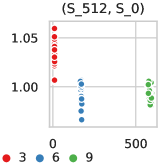
(a)

(b)

(c)

Figure 5: Number of crossings of the $k$-regular graphs.

Observe that the power, 11138_bus, ch7-6-b1 and commanche_d graphs all have an average vertex-degree of roughly $3.0$. The comparison of the number of crossing obtained by $\mathcal{S}_{512}$ and $\mathcal{S}_{0}$ is not conclusive, since $\mathcal{S}_{0}$ yields fewer crossings on the power and commanche_d graphs and $\mathcal{S}_{512}$ on the remaining two. In order to be able to further study the effect of the (average) vertex degree we evaluate the number of crossings of $k$-regular graphs. We use the plots in Figure 5 for the evaluation. Each point $(x_{G},y_{G})$ corresponds to a $k$-regular graph $G$. The color encodes the vertex-degree. Let $\Gamma_{A}$ and $\Gamma_{B}$ be two drawings of $G$ obtained by an algorithm $A$ and $B$, respectively. The $x$-value $x_{G}$ corresponds to the number of crossings in $\Gamma_{A}$ in thousands, i.e., $\operatorname{{\mathrm{cr}}}(\Gamma_{A})/1000$. The $y$-value $y_{G}$ is the quotient $\operatorname{{\mathrm{cr}}}(\Gamma_{B})/\operatorname{{\mathrm{cr}}}(\Gamma_{A})$. The titles of the plots are in the form $(A,B)$ and encode the compared algorithms. For example in Figure 5(a) algorithm $A$ is Stress and $B$ is $\mathcal{S}_{0}$. For example, the Stress drawings of the $3$-regular graphs have on average $12\,487$ crossings. Drawings obtained by $\mathcal{S}_{0}$ have on average $17\%$ less crossings, i.e., $10\,402$. On the other hand, $\mathcal{S}_{512}$ decreases the number of crossings on average by $20\%$. For $k=6,9$, $\mathcal{S}_{0}$ and $\mathcal{S}_{512}$ both reduce the number of crossings by $25\%$. In particular, Figure 5(c) shows that for $k=6,9$ it is unclear, whether $\mathcal{S}_{512}$ or $\mathcal{S}_{0}$ computes drawings with fewer crossings.

4.3 Weighted Sampling

For some graphs, the previous section gives first indications that sampling a set of edges yields a small number of crossings compared to a pure sampling of points in the plane. In particular Figure 5(c) indicates that the edge-sampling approach does not always have a clear advantage over sampling points in the plane. One reason for this might be that sampling within the set of points $P_{i}$ in the region $R_{i}$ is too restrictive. Observe that the region $R_{i}$ is only crossing-minimal with respect to the sample $S$ and does not necessarily contain the crossing-minimal position $p^{\star}_{i}$ of the vertex $v_{i}$ with respect to all edges $E$. On the other hand, sampling the set of points $P_{i}$ in $\mathbb{R}^{2}$ does not use the structure of the graph at all. This motivates the following weighted approach of sampling points in $\mathbb{R}^{2}$.

For a set $S\subset E$, let $\operatorname{{\mathrm{cr}}}_{j}$ be the number of crossings of the vertex $v_{i}$ with respect to $\Gamma|_{S}$, when $v_{i}$ is moved to a cell $c_{j}$ of the arrangement $\mathcal{A}(\Gamma|_{S},v_{i})$. Let $M$ be the maximum of all $\operatorname{{\mathrm{cr}}}_{j}$. We select a cell $c_{j}$ with the probability $2^{M-\operatorname{{\mathrm{cr}}}_{j}}/\sum_{k}2^{M-\operatorname{{\mathrm{cr}}}_{k}}$. Within a given cell, we draw a point uniformly at random. Note that in case that there are exactly $n$ cells such that cell $c_{j}$ induces $j$ crossings, the probability that the cell $c_{0}$ is drawn converges to $1/2$ for $n\rightarrow\infty$.

Benchmark Instances, Preprocessing & Methodology.

We use the same benchmark set and the same preprocessing steps as described in Section 4. In order to obtain more reliable results, we perform 10 independent iterations for each configuration on the Dimacs and Sparse MC graphs. Since the $k$-regular graphs are uniform randomly computed, they are already representative for their class. Therefore, we perform only single runs on these graphs.

Configuration.

We compare the following three configurations. $\mathcal{R}_{0}$ refers to the uniform random sampling of points in $\mathbb{R}^{2}$ with the parameters $(|S|,|P|,K)=(0,1000,\infty)$, $\mathcal{R}_{512}$ to the restricted sampling in $R_{i}$ with the parameters, $(512,1000,100)$, and $\mathcal{W}_{512}$ to the weighted sampling in $\mathbb{R}^{2}$ with the parameters $(512,1000,100)$. The configurations are selected such that $\mathcal{R}_{0}$ and $\mathcal{R}_{512}$ differ only in a single parameter, i.e., in the number of sampled edges. The only difference between $\mathcal{R}_{512}$ and $\mathcal{W}_{512}$ is the sampling strategy. Note that the parameters of $\mathcal{R}_{0}$ and $\mathcal{S}_{0}$ coincide, but not the parameters of $\mathcal{S}_{512}$ and $\mathcal{R}_{512}$.

Table 2: Mean and standard deviation (std) of the number of crossing categorized by configuration. For each graph the configuration with the lowest and highest number of crossings in marked.

	$\mathcal{R}_{0}$		$\mathcal{R}_{512}$		$\mathcal{W}_{512}$
	mean	std	mean	std	mean	std
Dimacs
adjnoun	4 445.0	39.55	3 655.7	62.96	3 951.2	19.53
football	3 973.6	97.93	3 350.0	83.38	3 247.0	73.84
netscience	819.0	30.73	497.1	28.78	437.8	12.87
c.metabolic	62 170.4	760.47	56 032.3	1 227.23	62 987.9	1 907.64
c.neural	89 744.3	1 239.22	86 500.8	1 364.5	99 426.1	1 258.98
jazz	152 013.8	1 930.13	147 387.1	3 134.15	213 019.4	1 696.07
power	6 301.1	33.51	4 512.8	63.09	3 912.5	30.97
email	356 583.4	3 512.0	341 503.8	3 480.74	351 168.7	2 624.18
hep-th	640 515.2	3 443.22	515 109.1	3 983.23	392 189.7	1 551.53
Sparse MC
1138_bus	474.6	13.25	342.9	12.91	247.6	9.8
ch7-6-b1	25 874.7	356.58	25 172.4	582.48	28 443.5	960.3
mk9-b2	251 360.9	1 514.05	245 447.4	2 914.18	228 794.5	2 069.96
bcsstk08	346 404.4	3 730.3	328 182.0	6 127.69	330 213.8	1 726.01
mahindas	1 036 745.7	11 494.88	936 889.0	11 207.34	1 105 850.9	10 185.51
eris1176	1 103 184.6	21 475.11	1 037 509.5	29 877.3	1 492 423.4	25 457.93
commanche_d	6 135.2	13.08	5 370.3	24.75	5 979.4	14.72

Evaluation.

Since we executed 10 independent runs of the algorithm on each graph, Table 2 lists the mean and standard deviation of the computed number of crossings for each graph. For each graph, we marked the cell with the lowest number of crossings in green and the largest number of crossings in blue. For each graph, we used the Mann-Witney-U test [22] to check the null hypothesis that the crossing numbers belong to the same distribution. The test indicates that we can reject the null hypothesis at a significance level of $\alpha=0.01$, for all graphs with the exception of football, ch7-6-b1 and bcsstk08. First, observe that the $\mathcal{R}_{0}$ configuration never computes a drawing with fewer crossings than $\mathcal{R}_{512}$. Including the football, ch7-6-b1 and the bcsstk08 graphs, $11$ of the drawings with the fewest crossing were obtained from the $\mathcal{R}_{512}$ configurations. Only $7$ correspond to the $\mathcal{W}_{512}$ configuration. Table 1 shows that these graphs have an average vertex-degree of at most 11. Moreover, Appendix A shows that the degree-distributions of these graphs follow the power-law. On the other hand, a few of the 8 graph where $\mathcal{R}_{512}$ outperforms $\mathcal{W}_{512}$ also have a small average vertex-degree.

(a)

(b)

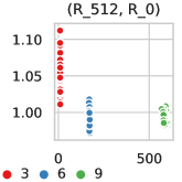
(c)

Figure 6: Comparison of the number of crossing of the $k$-regular graphs computed by $\mathcal{W}_{512}$ and $\mathcal{R}_{512}$.

We use Figure 6 to compare the effect of the vertex-degree on the number of crossings. The plot follows the same convention as the plots in Figure 5. Observe that for each $k$, the $\mathcal{W}_{512}$ configuration computes drawings with fewer crossings than $\mathcal{R}_{512}$. The improvement decreases with an increasing $k$. The same observation can be made for the comparison of $\mathcal{W}_{512}$ to $\mathcal{R}_{0}$ but not for the comparison for $\mathcal{R}_{512}$ to $\mathcal{R}_{0}$, which indicates that sampling the set of points $P_{i}$ within the region $R_{i}$ is indeed too restrictive, at least on our $k$-regular graphs.

Overall our experimental evaluation shows that even with a naive uniform random sampling of a set of points in the plane the number of crossings in drawings of Stress can be reduced considerably. Using a random sample of a subset of the edges helps to compute drawings with even less crossings. The mean-vertex degree and the degree-distributions are good indicators for whether the restrictive or the weighted sampling of the point set $P_{i}$ results in a drawing with the smallest number of crossings.

5 Conclusion

In our previous work we showed that the primitive operation of moving a single vertex to its crossing-minimal position significantly reduces the number of crossings compared to drawings obtained by Stress. In this paper we introduced the concept of bloated dual of line arrangements, a combinatorial technique to compute a dual representation of line arrangements. In our applications of computing drawings with a small number of crossings, this technique resulted in a speed-up of factor of $20$. This improvement was necessary to adapt the approach for graphs with a large number of vertices and edges. On the other hand, since the worst-case running time is super-quadratic, this improvement is not sufficient to cope with large graphs. In Section 4 we showed that random sampling is a promising technique to minimize crossings in geometric drawings. In Section 4.1 we proved that a random subset of edges of size $\Theta(k\log k)$ approximates the co-crossing number of a vertex $v$ with a high high probability. Further, we evaluated three different strategies to sample a set of points in the plane in order to compute a new position for the vertex $v_{i}$. First, the evaluation confirms that the number of crossings compared to Stress can be reduced considerably. Furthermore, sampling a small subset of the edges is sufficient to reduce the number of crossings compared to a naive sampling of points the plane. Our evaluation suggests that weighted sampling is a promising approach to reduce the number of crossings in graphs with a low average vertex degree. Otherwise, the evaluation indicates that restricted sampling results in fewer crossings.

The running time of the vertex-movement approach in combination with the sampling of the edges mostly depends on the number of vertices. Since a single movement of a vertex is not optimal anymore, two vertices can be moved independently. Thus, future research should be concerned with the question whether a parallelization over the vertex set is able to further reduce the running time while preserving the small number of crossings. Moreover, we ask whether it is sufficient to move a small subset of the vertices to considerably reduce the number of crossings.

Appendix A Degree Distribution

The plots in the Figures 7 to 9 show the degree distribution of the Dimacs and Sparse MC graphs that are listed in Table 1. A graph is listed in Figure 7 if the configuration $\mathcal{R}_{512}$ computed drawings with clearly less crossings than $\mathcal{W}_{512}$. In case that $\mathcal{W}_{512}$ computes a drawing with less crossings, then the graph is listed in Figure 8. If no distinction can be made, the graph is listed in Figure 9. Observe that all graphs in Figure 7 tend to have power-law distribution. The plots in Figure 7 and Figure 9 contains distributions that follow the power-follow but also distributions that tend to be normal or unstructured.

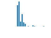
(a) adjnoun

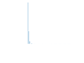
(b) celegans_metabolic

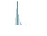
(c) celegansneural

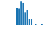
(d) jazz

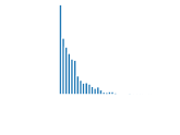
(e) email

(f) ch7-6-b1

(g) commanche_dual

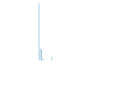
(h) mahindas

Figure 7: Degree distribution of graphs on which the $\mathcal{R}_{512}$ computes a small number of crossings.

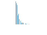
(a) netscience

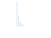
(b) power

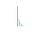
(c) hep-th

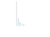
(d) 1138_bus

(e) mk9-b2

Figure 8: Degree distribution of graphs on which the $\mathcal{W}_{512}$ computes a small number of crossings.

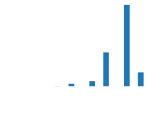
(a) football

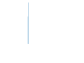
(b) bcsstk08

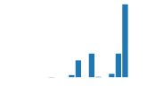
(c) bcsstk27

Figure 9: Degree distribution of the remaining graphs.

Appendix B Statistics of the $k$-regular

Table 3 lists the statistics that correspond to the plots in Figure 5.

Table 3: Mean Number of crossings and standard deviation of number of crossings in drawings of the $k$-regular graphs computed by $\mathcal{S}_{0}$ and Stress.

(a) $\mathcal{S}_{0}$ vs Stress

$k$	crossings $S_{0}$		crossings stress
	mean	std	mean	std
3	10 402.64	258.90	12 487.96	384.04
6	169 365.52	2260.86	227 303.68	3450.72
9	580 661.80	6333.13	774 791.92	8461.29

(b) $\mathcal{S}_{512}$ vs Stress

deg	crossings $S_{512}$		stress_crossings
	mean	std	mean	std
3	100 43.76	285.83	12 487.96	384.04
6	170 558.48	2379.56	227 303.68	3450.72
9	584 505.16	7393.01	774 791.92	8461.29

Appendix C Missing Proofs

See 4.2

Proof C.10.

In order to proof the claim, we make a case distinction based on the size of $R$. We first assume that $\lvert{S\cap X}\rvert/\lvert{S}\rvert<\lvert{R}\rvert/\lvert{X}\rvert$. Thus, we immediately get that $\lvert{X}\rvert\lvert{S\cap R}\rvert/\lvert{S}\rvert\leq|R|\leq(1+\delta)|R|$ Moreover, the following holds $\lvert{\lvert{S\cap R}\rvert/\lvert{S}\rvert-\lvert{R}\rvert/\lvert{X}\rvert}\rvert=\lvert{R}\rvert/\lvert{X}\rvert-\lvert{S\cap R}\rvert/\lvert{S}\rvert$. Starting from the fact $S$ is $(\varepsilon,\delta)$-approximation, we can do the following transformations.

$$\left|{X}\right|\left(\frac{\left|{R}\right|}{\left|{X}\right|}-\frac{\left|{S\cap R}\right|}{\left|{S}\right|}\right)\leq\delta\lvert{X}\rvert\max\left\{\frac{\left|{R}\right|}{\left|{X}\right|},\varepsilon\right\}$$

$$\Leftrightarrow \left|{R}\right|-\left|{X}\right|\frac{\left|{S\cap R}\right|}{\left|{S}\right|}\leq\delta\max\left\{\left|{R}\right|,\varepsilon\left|{X}\right|\right\}$$

$$\Leftrightarrow \left|{X}\right|\frac{\left|{S\cap R}\right|}{\left|{S}\right|}\geq\left|{R}\right|-\delta\left|{R}\right|=(1-\delta)\left|{R}\right|$$

In order to complete the proof, assume that $\lvert{S\cap X}\rvert/\lvert{S}\rvert\geq\lvert{R}\rvert/\lvert{X}\rvert$.

$$\left|{X}\right|\left(\frac{\left|{S\cap R}\right|}{\left|{S}\right|}-\frac{\left|{R}\right|}{\left|{X}\right|}\right)\leq\delta\lvert{X}\rvert\max\left\{\frac{\left|{R}\right|}{\left|{X}\right|},\varepsilon\right\}$$

$$\Leftrightarrow \left|{R}\right|-\left|{X}\right|\frac{\left|{S\cap R}\right|}{\left|{S}\right|}\leq\delta\max\left\{\left|{R}\right|,\varepsilon\left|{X}\right|\right\}$$

$$\Leftrightarrow \left|{X}\right|\frac{\left|{S\cap R}\right|}{\left|{S}\right|}\leq\left|{R}\right|+\delta\left|{R}\right|=(1+\delta)\left|{R}\right|$$

See 4.6

Proof C.11.

Recall that $\operatorname{{\mathrm{co-cr}}}(p)$ is equal to $\sum_{u\in N(v)}\lvert{{\overline{{\mathbb{E}_{uv}(p)}}}}\rvert$. Since the drawing $\Gamma$ is $\varepsilon$-well behaved, for every $u\in N(v)$ and every $p\in\mathbb{R}^{2}$ we have that at least an $\varepsilon$-fraction of edges is not crossed by the edge $uv$, i.e., $\lvert{{\overline{{\mathbb{E}_{uv}(p)}}}}\rvert\geq\varepsilon|E|$. Since $S_{u}$ is a relative $(\varepsilon,\delta)$-approximation and due to Proposition 4.2 we have that $(1-\delta)|{\overline{{\mathbb{E}_{uv}(p)}}}|\leq|E||{\overline{{\mathbb{E}_{uv}(p)}}}\cap S_{u}|/|S_{u}|\leq(1+\delta)|{\overline{{\mathbb{E}_{uv}(p)}}}|$. Plugging this inequality into the sum of $\lambda(p)$ proves the lemma.

See 4.7

Proof C.12.

For each vertex $u\in N(v)$, we denote with $A_{u}$ the event that $S$ is a relative $(\varepsilon,\delta)$-approximation of the set system $(E,\overline{\mathcal{F}_{uv}})$. According to Lemma 4.4 and Theorem 4.3 the probability $\operatorname*{\mathbb{P}}(A_{u})$ that a uniformly random sample is a relative $(\varepsilon,\delta)$-approximation of $(E,\overline{\mathcal{F}_{uv}})$ is $1-\gamma$. The following estimate can be proven by induction using the equalities $\operatorname*{\mathbb{P}}(A\wedge B)=\operatorname*{\mathbb{P}}(A)+\operatorname*{\mathbb{P}}(B)-\operatorname*{\mathbb{P}}(A\vee B)$ and $\operatorname*{\mathbb{P}}(A\vee B)\leq 1$.

$$\operatorname*{\mathbb{P}}\left(\bigwedge_{u\in N(v)}A_{u}\right)\geq\sum_{u\in N(v)}\operatorname*{\mathbb{P}}(A_{u})-k+1$$

Plugging in the probability for $\operatorname*{\mathbb{P}}(A_{u})$ proves that $S$ is a relative $(\varepsilon,\delta)$-approximation with probability $1-k\gamma$ for a $\gamma\leq 1/k$.

References

- [1] Oswin Aichholzer. On the Rectilinear Crossing Number. (http://www.ist.tugraz.at/staff/aichholzer/research/rp/triangulations/crossing), 5 2017.
- [2] David A. Bader, Andrea Kappes, Henning Meyerhenke, Peter Sanders, Christian Schulz, and Dorothea Wagner. Benchmarking for Graph Clustering and Partitioning. In Encyclopedia of Social Network Analysis and Mining, 2nd Edition. Springer-Verlag, 2018. doi:10.1007/978-1-4939-7131-2\_23.
- [3] Michael A. Bekos, Henry Förster, Christian Geckeler, Lukas Holländer, Michael Kaufmann, Amadäus M. Spallek, and Jan Splett. A Heuristic Approach Towards Drawings of Graphs with High Crossing Resolution. In Proceedings of the 26th International Symposium on Graph Drawing (GD’18), volume 11282 of Lecture Notes in Computer Science, pages 271–285, 2018. doi:10.1007/978-3-030-04414-5\_19.
- [4] John L. Bentley and Thomas A. Ottmann. Algorithms for Reporting and Counting Geometric Intersections. IEEE Transactions on Computers, C-28(9):643–647, 1979.
- [5] Daniel Bienstock. Some Provably Hard Crossing Number Problems. Discrete & Computational Geometry, 6(1):443–459, 1991. doi:10.1007/BF02574701.
- [6] Christoph Buchheim, Markus Chimani, Carsten Gutwenger, Michael Jünger, and Petra Mutzel. Crossings and Planarization. In Roberto Tamassia, editor, Handbook of Graph Drawing and Visualization, chapter 2, pages 43–85. Chapman and Hall/CRC, 2013.
- [7] Markus Chimani, Carsten Gutwenger, Michael Jünger, Gunnar W. Klau, Karsten Klein, and Petra Mutzel. The Open Graph Drawing Framework (OGDF). In Roberto Tamassia, editor, Handbook of Graph Drawing and Visualization, chapter 17, pages 543–569. Chapman and Hall/CRC, 2013.
- [8] Markus Chimani and Petr Hlinený. Inserting Multiple Edges into a Planar Graph. In Sándor Fekete and Anna Lubiw, editors, Proceedings of the 32nd Annual Symposium on Computational Geometry (SoCG’16), volume 51 of Leibniz International Proceedings in Informatics (LIPIcs), pages 30:1–30:15. Schloss Dagstuhl–Leibniz-Zentrum fuer Informatik, 2016. doi:10.4230/LIPIcs.SoCG.2016.30.
- [9] Timothy A. Davis and Yifan Hu. The University of Florida Sparse Matrix Collection. ACM Transactions on Mathematical Software, 38(1):1:1–1:25, 2011. doi:10.1145/2049662.2049663.
- [10] Almut Demel, Dominik Dürrschnabel, Tamara Mchedlidze, Marcel Radermacher, and Lasse Wulf. A Greedy Heuristic for Crossing-Angle Maximization. In Proceedings of the 26th International Symposium on Graph Drawing (GD’18), Lecture Notes in Computer Science, pages 286–299, 2018. doi:10.1007/978-3-030-04414-5\_20.
- [11] Ruy Fabila-Monroy and Jorge López. Computational Search of Small Point Sets with Small Rectilinear Crossing Number. Journal of Graph Algorithms and Applications, 18(3):393–399, 2014. doi:10.7155/jgaa.00328.
- [12] Emden R. Gansner, Yehuda Koren, and Stephen North. Graph Drawing by Stress Majorization. In János Pach, editor, Proceedings of the 12th International Symposium on Graph Drawing (GD’04), volume 3383 of Lecture Notes in Computer Science, pages 239–250. Springer Berlin/Heidelberg, 2005. doi:10.1007/978-3-540-31843-9\_25.
- [13] Michael R. Garey and David S. Johnson. Crossing Number is NP-Complete. SIAM Journal on Algebraic and Discrete Methods, 4(3):312–316, 1983.
- [14] Carsten Gutwenger, Petra Mutzel, and René Weiskircher. Inserting an Edge into a Planar Graph. Algorithmica, 41(4):289–308, 2005. doi:10.1007/s00453-004-1128-8.
- [15] Sariel Har-Peled and Micha Sharir. Relative -Approximations in Geometry. Discrete & Computational Geometry, 45(3):462–496, 2011. doi:10.1007/s00454-010-9248-1.
- [16] Stephen G. Kobourov. Force-Directed Drawing Algorithms. In Roberto Tamassia, editor, Handbook of Graph Drawing and Visualization, chapter 12. Chapman and Hall/CRC, 2013.
- [17] Yi Li, Philip M. Long, and Aravind Srinivasan. Improved Bounds on the Sample Complexity of Learning. Journal of Computer and System Sciences, 62(3):516 – 527, 2001. doi:10.1006/jcss.2000.1741.
- [18] Jiří Matoušek. Lectures on Discrete Geometry, volume 212. Springer New York, 2002.
- [19] Henning Meyerhenke, Martin Nöllenburg, and Christian Schulz. Drawing Large Graphs by Multilevel Maxent-Stress Optimization. IEEE Transactions on Visualization and Computer Graphics, 24(5):1814–1827, 2018. doi:10.1109/TVCG.2017.2689016.
- [20] Thomas L. Moore. Using Euler’s Formula to Solve Plane Separation Problems. The College Mathematics Journal, 22(2):125–130, 1991.
- [21] Marcel Radermacher, Klara Reichard, Ignaz Rutter, and Dorothea Wagner. A Geometric Heuristic for Rectilinear Crossing Minimization. In Proceedings of the 20th Workshop on Algorithm Engineering and Experiments (ALENEX’18), pages 129–138, 2018. doi:10.1137/1.9781611975055.12.
- [22] David J. Sheskin. Handbook of Parametric and Nonparametric Statistical Procedures. Chapman and Hall/CRC, 2003.
- [23] Angelika Steger and Nicholas C. Wormald. Generating Random Regular Graphs Quickly. Combinatorics, Probability and Computing, 8(4):377–396, 1999.
- [24] The CGAL Project. CGAL User and Reference Manual (http://doc.cgal.org/4.10/Manual/packages.html). CGAL Editorial Board, 4.10 edition, 2017.
- [25] Vladimir N. Vapnik and Alexey Y. Chervonenkis. On the Uniform Convergence of Relative Frequencies of Event to their Probabilities. Theory of Probability & Its Application, 16(2):264–280, 1971.
- [26] Imrich Vrt’o. Bibliography on Crossing Numbers of Graphs. (ftp://ftp.ifi.savba.sk/pub/imrich/crobib.pdf), 2014.