Hadron-Hadron Interactions from $N_{f}=2+1+1$ Lattice QCD:
The $\rho\,$-resonance

Abstract

We present a lattice QCD investigation of the $\rho$-meson with $N_{f}=2+1+1$ dynamical quark flavours for the first time. The calculation is performed based on gauge configuration ensembles produced by the ETM collaboration with three lattice spacing values and pion masses ranging from $230\ \mathrm{MeV}$ to $500\ \mathrm{MeV}$. Applying the Lüscher method phase shift curves are determined for all ensembles separately. Assuming a Breit-Wigner form, the $\rho$-meson mass and width are determined by a fit to these phase shift curves. Mass and width combined are then extrapolated to the chiral limit, while lattice artefacts are not detectable within our statistical uncertainties. For the $\rho$-meson mass extrapolated to the physical point we find good agreement with experiment. The corresponding decay width differs by about two standard deviations from the experimental value.

1 Introduction

The $\rho$-meson represents together with the (in-)famous $\sigma$-meson ($f_{0}(500)$) one of the most prominent meson resonances in the standard model. The $\rho$ decays almost exclusively to two pions and the experimental phase shift curve Erwin:1961ny ; Protopopescu:1973sh is a textbook example for a relativistic Breit-Wigner form. Moreover, the $\rho$, being the lightest vector meson, plays a fundamental role in many processes within the context of vector meson dominance, for a review see Ref. Meissner:1987ge .

Therefore, an investigation of the $\rho$-meson properties from first principles with lattice QCD is highly desirable. However, unstable particles require special care in lattice QCD: interaction properties can only be computed using the by now famous Lüscher method Luscher:1985dn ; Luscher:1986pf ; Luscher:1990ux . With its help, infinite volume scattering properties can be extracted from finite volume energy shifts. In the meanwhile the Lüscher method has been developed further in many directions, for a review see Ref. Briceno:2017max , in particular also for three particle systems, see for instance Refs. Polejaeva:2012ut ; Briceno:2018aml ; Romero-Lopez:2018rcb ; Pang:2019dfe ; Hansen:2019nir ; Mai:2017bge . For this paper most relevant is the derivation of the formalism in moving frames Rummukainen:1995vs ; Feng:2010es ; Gockeler:2012yj , which allows one to map out the phase shift at many different scattering momenta, without the need to study different volumes.

For a long time the Lüscher method was difficult to apply to the $\rho$ in realistic lattice calculations, albeit there are some early attempts McNeile:2002fh ; Michael:2006hf . By now, there are a number of investigations of the $\rho$-meson from lattice QCD using the Lüscher method Feng:2010es ; Lang:2011mn ; Aoki:2011yj ; Dudek:2012xn ; Bali:2015gji ; Wilson:2015dqa ; Fu:2016itp ; Guo:2016zos ; Alexandrou:2017mpi ; Andersen:2018mau . The first computation with light dynamical up and down quarks can be found in the pioneering work of Ref. Feng:2010es . Subsequent investigations focused on different aspects like large operator bases Dudek2013 or asymmetric boxes Guo:2016zos . Recently, a first investigation involving different lattice spacings and a range of pion masses has been performed Andersen:2018mau . However, in the latter reference chiral and continuum extrapolations were not performed.

With this paper we fill this gap and present a computation of the $\rho$-meson applying the Lüscher method using gauge ensembles generated with $N_{f}=2+1+1$ dynamical quark flavours by the ETM collaboration at three different lattice spacing values and a wide range of pion masses Baron:2010bv ; Baron:2010th . This allows us to perform a chiral and continuum extrapolation of the $\rho$-meson mass and width. Note that in Ref. Giusti:2018mdh the mass and width of the $\rho$-meson has been determined on the same gauge configurations, however, using an inverse Lüscher approach based on the vector current only combined with a parametrisation of the pion form factor.

This paper is organised as follows: after presenting the lattice action and its parameters in section 2, we discuss our methods in section 3. In section 4 we present our results, the main result being the continuum extrapolated values of $M_{\rho}$ and $\Gamma_{\rho}$ at the physical pion mass value reading

$$M_{\rho}\ =\ 769(19)\ \mathrm{MeV}\,,\qquad\Gamma_{\rho}\ =\ 129(7)\ \mathrm{MeV}\,.$$

In section 5 we discuss our results and put them into perspective, followed by a summary in section 6. More technical details can be found in the appendix.

2 Lattice Action

The lattice details for the investigation presented here are very similar to those we used in our previous studies on hadron-hadron interactions Helmes:2015gla ; Helmes:2017smr ; Helmes:2018nug ; Helmes:2019dpy . We use $N_{f}=2+1+1$ flavour lattice QCD ensembles generated by the ETM Collaboration, for which details can be found in Refs. Chiarappa:2006ae ; Baron:2010th ; Baron:2010bv . The parameters relevant for this paper are compiled in Table 1: we give for each ensemble the inverse gauge coupling $\beta=6/g_{0}^{2}$, the bare values for the quark mass parameters $\mu_{\ell},\mu_{\sigma}$ and $\mu_{\delta}$, the lattice volume and the number of configurations on which we estimated the relevant quantities.

ensemble	$\beta$	$a\mu_{\ell}$	$a\mu_{\sigma}$	$a\mu_{\delta}$	$(L/a)^{3}\times T/a$	$N_{\mathrm{conf}}$
A30.32	$1.90$	$0.0030$	$0.150$	$0.190$	$32^{3}\times 64$	$623$
A40.24	$1.90$	$0.0040$	$0.150$	$0.190$	$24^{3}\times 48$	$997$
A40.32	$1.90$	$0.0040$	$0.150$	$0.190$	$32^{3}\times 64$	$493$
A60.24	$1.90$	$0.0060$	$0.150$	$0.190$	$24^{3}\times 48$	$618$
A80.24	$1.90$	$0.0080$	$0.150$	$0.190$	$24^{3}\times 48$	$611$
A100.24	$1.90$	$0.0100$	$0.150$	$0.190$	$24^{3}\times 48$	$307$
B25.32	$1.95$	$0.0025$	$0.135$	$0.170$	$32^{3}\times 64$	$197$
B35.32	$1.95$	$0.0035$	$0.135$	$0.170$	$32^{3}\times 64$	$493$
B35.48	$1.95$	$0.0035$	$0.135$	$0.170$	$48^{3}\times 96$	$265$
B55.32	$1.95$	$0.0055$	$0.135$	$0.170$	$32^{3}\times 64$	$613$
D15.48	$2.10$	$0.0015$	$0.120$	$0.1385$	$48^{3}\times 96$	$304$
D30.48	$2.10$	$0.0030$	$0.120$	$0.1385$	$48^{3}\times 96$	$241$
D45.32sc	$2.10$	$0.0045$	$0.0937$	$0.1077$	$32^{3}\times 64$	$588$

Table 1: The gauge ensembles used in this study. For the labeling of the ensembles we adopted the notation in Ref. Baron:2010bv . In addition to the relevant input parameters we give the lattice volume and the number of evaluated configurations, $N_{\mathrm{conf}}$.

The ensembles were generated using the $N_{f}=2+1+1$ twisted mass fermion action Frezzotti:2003ni ; Frezzotti:2003xj ; Frezzotti:2004wz . For orientation, the $\beta$-values $1.901.952.10$ correspond to lattice spacing values of $a\sim\,0.089\ \mathrm{fm},0.082\ \mathrm{fm}$ and $a\sim\,0.062\ \mathrm{fm}$, respectively, see also Table 2. The ensembles were generated at so-called maximal twist, which guarantees automatic order $\order{a}$ improvement for almost all physical quantities Frezzotti:2003ni . The corresponding lattice Dirac operator in the light sector reads

$$D^{\mathrm{tm}}_{\ell}\ =\ D_{\mathrm{W}}+m_{\mathrm{cr}}+i\mu_{\ell}\gamma_{5}\tau^{3}\,,$$ (1)

with $D_{\mathrm{W}}$ the Wilson Dirac operator, $m_{\mathrm{cr}}$ the Wilson quark mass tuned to its critical value, $\mu_{\ell}$ the bare up/down quark mass parameter and $\tau^{3}$ the third Pauli matrix acting in flavour space. The tuning of the Wilson quark mass to its critical value is discussed in Ref. Baron:2010bv , where also the Dirac operator for the strange/charm sector can be found, which is not relevant for the remainder of this paper. The relation of the bare parameters $\mu_{\sigma}$ and $\mu_{\delta}$ given in Table 1 are related to the renormalised strange and charm quark masses as follows:

$$m_{s,c}\ =\ \frac{1}{Z_{P}}\mu_{\sigma}\mp\frac{1}{Z_{S}}\mu_{\delta}\,.$$

The bare strange and charm quark masses are kept constant for each $\beta$-value. The renormalised strange quark mass values differ from the physical one by up to 10%, see Ref. Baron:2010bv ; Baron:2010th ; Carrasco:2014cwa for details. In our chiral and continuum extrapolation we treat the strange quark mass as constant in spite of this deviation. In the gauge sector the Iwasaki action is used Iwasaki:1983ck ; Iwasaki:1984cj .

The biggest disadvantage of Wilson twisted mass fermions at maximal twist is the breaking of isospin symmetry. As a consequence, charged and neutral pions are not mass degenerate, with the splitting in the squared masses vanishing like $a^{2}$ towards the continuum limit. This pion mass splitting is also about the only quantity where strong effects of isospin splitting have been observed so far Herdoiza:2013sla .

We are going to study the decay $\rho^{0}\to\pi^{+}\pi^{-}$ in a $p$-wave. In nature, there is no mixing with two neutral pions possible. Even if there is reduced isospin symmetry (only $I_{z}$ is a good quantum number) in the Wilson twisted mass formulation at maximal twist, such mixing is still not possible due to $C$-symmetry: $\rho^{0}$ is $C$-odd, while $\pi^{0}\pi^{0}$ is $C$-even. Likewise, non $p$-wave symmetric combinations of $\pi^{+}\pi^{-}$ are $C$-even, while $p$-wave symmetric combinations of $\pi^{+}\pi^{-}$ are $C$-even, for instance

$$\begin{split}O^{l=0,1}&=\pi^{+}(p_{1})\pi^{-}(p_{2})+(-1)^{l}\pi^{-}(p_{1})\pi^{+}(p_{2})\\ C\,O^{l=0,1}\,C^{-1}&=\pi^{-}(p_{1})\pi^{+}(p_{2})+(-1)^{l}\pi^{+}(p_{1})\pi^{-}(p_{2})\\ &=(-1)^{l}O^{l=0,1}\,,\\ \end{split}$$

excluding also mixings with $I=2,I_{z}=0$ states. Moreover, also a single $\pi^{0}$ is $C$-even and cannot mix.

However, due to missing isospin symmetry, there are fermionic disconnected contributions to the $\rho^{0}$ lattice interpolating operators. These can be shown, like for the neutral pion, to be purely of $\mathcal{O}(a^{2})$. Thus, we drop them from our calculation, as was also done in Ref. Feng:2010es . Note that the neutral to charged $\rho$-meson splitting was found to be negligible Michael:2007vn .

As a smearing and contraction scheme we employ the stochastic Laplacian-Heaviside (sLapH) approach, described in Ref. Morningstar:2011ka . Details of our sLapH parameter choices can be found in Refs. Helmes:2015gla ; Helmes:2017smr .

$\beta$	$a\ [\mathrm{fm}]$	$r_{0}/a$
$1.90$	$0.0885(36)$	$5.31(8)$
$1.95$	$0.0815(30)$	$5.77(6)$
$2.10$	$0.0619(18)$	$7.60(8)$

Table 2: Values of the Sommer parameter $r_{0}/a$ and the lattice spacing $a$ at the three values of $\beta$. See Ref. Carrasco:2014cwa for more details.

2.1 Scale Setting

The scale setting for the ensembles used here has been performed in Ref. Carrasco:2014cwa by extrapolating pseudo-scalar meson masses and decay constants to the chiral and continuum limits and using the physical values of $M_{\pi}$ and $f_{\pi}$ as inputs. As an intermediate scale the Sommer parameter $r_{0}/a$ has been used. The values for the lattice spacings resulting from this procedure can be found in Table 2 together with the values of $r_{0}/a$ for each $\beta$-value. The physical value of the Sommer parameter was determined in Ref. Carrasco:2014cwa on the same ensembles as the value

$$r_{0}=0.474(11)\ \mathrm{fm}\,.$$ (2)

In this paper we are also going to use the Sommer parameter as intermediate lattice scale. In addition to the physical value for $r_{0}$ given above we need the physical pion mass value as input. Here, we use the value of $M_{\pi}$ in the isospin symmetric limit Aoki:2016frl (consistent with what was used in Ref. Carrasco:2014cwa )

$$\overline{M}_{\pi^{+}}\ =\ 134.8(3)\ \mathrm{MeV}$$ (3)

corrected for QED and strong isospin contributions. The values of $r_{0}/a$ were not determined by us on the identical set of gauge configurations. Therefore, we use the values given in Table 2 with re-sampling (parametric bootstrap). $\overline{M}_{\pi}$ and its error are treated in the same way.

In the appendix B we discuss how we include uncertainties on $r_{0}/a$, $\overline{M}_{\pi^{+}}$ and other input. We remark that at fixed $\beta$-value there is in principle correlation between $r_{0}/a$ and all other observables. However, we cannot take these correlations into account, because $r0/a$ was not determined on the identical gauge configurations. However, we measured this correlation to more precisely estimated quantities like $aM_{\pi}$ previously and found the correlation to be negligible.

3 Methods

In this section we summarise the methodology we applied to extract our results.

3.1 Scattering in Finite Volume

As is well known, the extraction of scattering properties from lattice QCD in Euclidean space-time and a finite volume requires the application of the so-called Lüscher method Luscher:1986pf ; Luscher:1990ux . It allows one to relate finite volume induced energy shifts to infinite volume scattering properties of $n$-particle systems in the continuum. The formalism is based on the following determinant equation

$$\det\left(M_{lm,l^{\prime}m^{\prime}}(k)-\delta_{ll^{\prime}}\delta_{mm^{\prime}}\cot(\delta_{l})\right)=0\,,$$ (4)

where $M_{lm,l^{\prime}m^{\prime}}$ is an analytically known matrix function of the lattice scattering momentum $k$, see below. $\delta_{l}$ is the phase shift of the $l$-th partial wave and the determinant acts in angular momentum space. In the case of pion-pion scattering the lattice scattering momentum $k$ is related to a given energy value $E_{\mathrm{CM}}$ in the centre-of-mass (CM) frame and the pion mass $M_{\pi}$ via

$$k^{2}\ =\ \frac{E_{\mathrm{CM}}^{2}}{4}-M_{\pi}^{2}\,.$$ (5)

Given the scattering momentum on the lattice, Eq. (4) thus yields $\delta_{l}$. In order to map out the dependence of $\delta_{l}$ on $E_{\mathrm{CM}}$, as many values of $E_{\mathrm{CM}}$ as possible must be extracted from a lattice calculation.

This is most conveniently done by using several CM momenta, as first proposed in Ref. Rummukainen:1995vs . For given CM momentum $\bm{p}_{\text{cm}}$, the relativistic energy reads

$$W_{\text{L}}=\sqrt{\bm{p}_{\text{cm}}^{2}+E_{\text{CM}}^{2}}$$ (6)

where $\bm{p}_{\text{cm}}$ is, due to the finite volume, quantised as

$$\bm{p}_{\text{cm}}=\frac{2\pi}{L}\cdot\bm{d}\,,\quad\bm{d}\in\mathbb{Z}^{3}\,.$$

We classify momentum sectors by $\absolutevalue{\bm{d}}^{2}$ and use all allowed lattice momenta in each sector up to $\mathbf{d}^{2}=4$. We denote the set of equivalent momenta as

$$\{\bm{d}\}\equiv\{\bm{z}\in\mathbb{Z}^{3}\,,\quad{\bm{z}}^{2}=\bm{d}^{2}\}\,.$$

By applying a corresponding Lorentz boost

$$\gamma\ =\ \frac{W_{\text{L}}}{E_{\mathrm{CM}}}\,,$$

we can compute $E_{\mathrm{CM}}$ for given $W_{L}$ and $\bm{p}_{\text{cm}}$. Adopting the notation of Refs. Bernard:2008ax ; Gockeler:2012yj , it remains to give details for the matrix $M$ from Eq. (4). Its matrix elements are given by

$$M_{lm,l^{\prime}m^{\prime}}=(-1)^{l}\sum_{j=\absolutevalue{l-l^{\prime}}}^{l+l^{\prime}}\sum_{s=-j}^{j}\sqrt{2j+1}\,i^{j}w_{js}C_{lm,js,l^{\prime}m^{\prime}}\,,$$ (7)

with the convenient notation

$$w_{js}=\frac{\mathcal{Z}_{js}(1,q^{2})}{\pi^{3/2}\sqrt{2j+1}\gamma q^{j+1}}\,,\qquad q=\frac{kL}{2\pi}\,.$$ (8)

$C_{lm,js,l^{\prime}m^{\prime}}$ represent coefficients which can be expressed using Wigner $3j$-symbols, see Ref. Gockeler:2012yj .

In a finite volume the symmetry group of rotoflections (rotations and space inversions) is reduced from $\mathrm{O}(3)$ to a finite subgroup. Because $\bm{p}_{\text{cm}}$ is an invariant, the group is different for each momentum sector.

In general, an irreducible representation restricted to a subgroup does not remain irreducible. The decomposition of the lowest partial waves is well known in the literature for all momentum sectors in this work Johnson1982 ; Mandula1983 ; Mandula1984 ; Moore:2005dw ; Moore:2006ng ; Bernard:2008ax ; Gockeler:2012yj .

The prescription to decompose an eigenstate of the $l$-th partial wave is often referred to as “subduction”. To introduce notation, assume the irrep $\mathrm{D}^{l}$ decomposes into a direct sum of different irreps $\Gamma_{i}$ each of which appears $n_{i}$ times such that

$$\mathrm{D}^{l}\to\bigoplus_{i}n_{i}\Gamma_{i}\,,\qquad\sum_{i}\ n_{i}\cdot\dim(\Gamma_{i})=2l+1\,.$$ (9)

Let $\Gamma\in\{\Gamma_{i}\}$, and label the basis vectors of $\Gamma$ by $\alpha\in\{1,\dots,\dim(\Gamma)\}$. The decomposition can be completely described by a set of “subduction coefficients” denoted by $s$. Given a basis $\{\ket{l,m}|-l\leq m\leq l\}$, the $\alpha$-th basis vector of the $n$-th copy of $\Gamma$ is given by

$$\ket{\Gamma\alpha ln}=\sum_{m}s_{lm}^{\Gamma\alpha n}\ket{lm}\,.$$ (10)

The derivation of subduction coefficients is discussed in appendix A. Applying the subduction to the matrix $M$ from Eq. (7) yields

$$M_{ln,l^{\prime}n^{\prime}}^{\Gamma} =\delta_{\Gamma\Gamma^{\prime}}\delta_{\alpha\alpha^{\prime}}\sum_{mm^{\prime}}{s_{lm}^{\Gamma\alpha n}}^{*}s_{l^{\prime}m^{\prime}}^{\Gamma^{\prime}\alpha^{\prime}n^{\prime}}M_{lm,l^{\prime}m^{\prime}}$$ (11)

$$=\sum_{mm^{\prime}}{s_{lm}^{\Gamma\alpha n}}^{*}s_{l^{\prime}m^{\prime}}^{\Gamma\alpha n^{\prime}}(-1)^{l}$$ (12)

$$\quad\times\sum_{j=\absolutevalue{l-l^{\prime}}}^{l+l^{\prime}}\sum_{s=-j}^{j}\sqrt{2j+1}i^{j}w_{js}C_{lm,js,l^{\prime}m^{\prime}}\,.$$ (13)

The Lüscher formula Eq. (4) remains formally unchanged except for the space it acts in. In the following, we will neglect all partial waves apart from the $p$-wave. In this case $n_{i}=1$ for all $i$ and Eq. (4) simplifies to

$$\delta_{1}=\arccot{M_{11,11}^{\Gamma}}\,,$$ (14)

The contributions of higher odd partial waves have been analysed and found to be negligible Dudek:2012xn ; Guo:2016zos . While twisted mass breaks parity and thus even partial waves may enter, the effect is suppressed by $\order{a^{2}}$ and also neglected here.

In Table 3 we list the explicit expressions for $M_{11,11}^{\Gamma}$ used in this work.

$\bm{d}^{2}$	$\Gamma$	$M_{11,11}^{\Gamma}$
$0$	$\mathrm{T1u}$	$w_{0,0}-w_{2,0}-\frac{3}{\sqrt{6}}w_{2,-2}-\frac{3}{\sqrt{6}}\cdot w_{2,2}$
$1$	$\mathrm{A1}$	$w_{0,0}+2\cdot w_{2,0}$
$1$	$\mathrm{E}$	$w_{0,0}-w_{2,0}+\frac{3i}{\sqrt{6}}\cdot w_{2,-2}-\frac{3i}{\sqrt{6}}\cdot w_{2,2}$
$2$	$\mathrm{A1}$	$w_{0,0}-w_{2,0}+\frac{3i}{\sqrt{6}}\cdot w_{2,-2}-\frac{3i}{\sqrt{6}}i\cdot w_{2,2}$
$2$	$\mathrm{B1}$	$w_{0,0}+2\cdot w_{2,0}$
$2$	$\mathrm{B2}$	$w_{0,0}-w_{2,0}-\frac{3i}{\sqrt{6}}\cdot w_{2,-2}+\frac{3i}{\sqrt{6}}\cdot w_{2,2}$
$3$	$\mathrm{A1}$	$w_{0,0}+2\cdot\frac{1+i}{\sqrt{6}}\cdot w_{2,-1}-2\cdot\frac{1-i}{\sqrt{6}}\cdot w_{2,1}+\frac{2i}{\sqrt{6}}\cdot w_{2,-2}-\frac{2i}{\sqrt{6}}\cdot w_{2,2}$
$3$	$\mathrm{E}$	$w_{0,0}-\frac{1+i}{\sqrt{6}}\cdot w_{2,-1}+\frac{1-i}{\sqrt{6}}\cdot w_{2,1}-\frac{i}{\sqrt{6}}\cdot w_{2,-2}+\frac{i}{\sqrt{6}}\cdot w_{2,2}$
$4$	$\mathrm{A1}$	$w_{0,0}+2\cdot w_{2,0}$
$4$	$\mathrm{E}$	$w_{0,0}-w_{2,0}+\frac{3i}{\sqrt{6}}\cdot w_{2,-2}-\frac{3i}{\sqrt{6}}\cdot w_{2,2}$

Table 3: Matrix elements for all momentum sectors $\bm{d}^{2}$ and irreps $\Gamma$ used in this work Bernard:2008ax .

3.2 Extraction of Energy Levels

In order to be able to use Eq. (14), we need to extract interacting energy levels for a given lattice irrep $\Gamma$ as well as the pion energy $E_{\pi}(\bm{p})$. The latter is, as usual, determined from the Euclidean time dependence of two-point functions

$$C_{\pi}(t-t^{\prime})\ =\ \langle\mathcal{O}_{\mathup{{{\pi}}^{\scriptstyle{+}}}}(t,\bm{p})^{\dagger}\ \mathcal{O}_{\mathup{{{\pi}}^{\scriptstyle{+}}}}(t^{\prime},\bm{p})\rangle$$ (15)

with operators $\mathcal{O}_{\mathup{{{\pi}}^{\scriptstyle{+}}}}(t,\bm{p})$ coupling to the charged pion state with momentum $\bm{p}$, see below. Note that in our formulation we have $M_{\pi^{+}}=M_{\pi^{-}}$. The spectral decomposition of $C_{\pi}$ yields

$$C_{\pi}(t)\ \propto\ \sum_{n}\left(\mathrm{e}^{-E_{n}t}+\mathrm{e}^{-E_{n}\,(T-t)}\right)\,.$$ (16)

In the limit of large Euclidean times only the ground states survives and allows one to extract $E_{\pi}(\bm{p})$ from its exponential decay.

For irrep $\Gamma$ we define a list of suitable operators $\mathcal{O}_{\Gamma}^{i}(t,\mathbf{p})$, $i=1,\ldots,n$, which project to irrep $\Gamma$ for momentum $\mathbf{p}$. Because the eigenvalues of operators from the same momentum sector and irrep are degenerate up to statistical fluctuations, we compute the correlator matrix by averaging over all moving frames connected by an allowed lattice rotation and rows of the irrep

$$\begin{split}\mathcal{C}_{\Gamma,\bm{d}^{2}}(t-t^{\prime})\ &=\ \frac{1}{\absolutevalue{\{\bm{d}\}}}\sum_{\bm{p}\ \in\ \{\bm{d}\}}\frac{1}{\dim(\Gamma)}\\ &\quad\times\sum_{\alpha=1}^{\dim(\Gamma)}\langle\ \vec{\mathcal{O}}_{\Gamma}^{\alpha}(t,\mathbf{p})^{\dagger}\cdot\vec{\mathcal{O}}_{\Gamma}^{\alpha}(t^{\prime},\mathbf{p})\ \rangle\,,\\ \end{split}$$ (17)

where we defined $\vec{\mathcal{O}}_{\Gamma}^{\alpha}=(\mathcal{O}_{\Gamma 1}^{\alpha},\ldots,\mathcal{O}_{\Gamma n}^{\alpha})^{t}$. The correlator matrix $\mathcal{C}_{\Gamma\mathbf{d}^{2}}(t)$ is then analysed using the standard variational method Michael:1982gb ; Luscher:1990ck yielding eigenvalues $\lambda_{i}(t,t_{0})$ which, at large enough $t$-values, decay like

$$\lambda_{i}(t,t_{0})\ \propto\exp(-W_{i}(t-t_{0}))+\exp(-W_{i}(T-t+t_{0}))\,,$$ (18)

where we neglect thermal pollutions for the moment, see section 3.4. Here, $T$ is the time extent of the lattice and $W_{i}$ the $i$th energy level to be extracted. $t_{0}$ represents the reference time at which the generalised eigenvalue problem (GEVP) is seeded. The correction to Eq. (18) due to excited states reads at fixed $t_{0}$-value Luscher:1990ck

$$\varepsilon_{i}(t,t_{0})=O(e^{-\Delta W_{i}t})\,.$$ (19)

Here, $\Delta W_{i}$ is the energy difference of $W_{i}$ to the first state not resolved by the correlation matrix. For a detailed discussion see Ref. Blossier:2009kd .

3.3 Operator Construction

We start with interpolating operators for pions $\pi^{\pm}$ with definite isospin $\ket{1,\pm 1}_{I}$:

$$\begin{split}\mathcal{O}_{\mathup{{{\pi}}^{\scriptstyle{+}}}}(x)&=\bar{d}(x)_{\alpha}^{c}\Gamma^{\pi}_{\alpha\beta}u(x)_{\beta}^{c}\,,\\ \mathcal{O}_{\mathup{{{\pi}}^{\scriptstyle{-}}}}(x)&=\bar{u}(x)_{\alpha}^{c}\Gamma^{\pi}_{\alpha\beta}d(x)_{\beta}^{c}\,,\end{split}$$ (20)

where $u$ and $d$ denote Dirac spinors for an up and down quark, respectively. $\alpha$, $\beta$ denote spin and $c$ colour indices, and $\Gamma^{\pi}=i\gamma_{5}$.

For the $\rho$-meson, we have to construct operators projected to $I=1$. A single $\rho^{0}$ can be interpolated by the canonical anti symmetric combination of quarks with isospin $\ket{1,0}_{I}$:

$$\mathcal{O}_{\mathup{{{\rho}}}}(x)=\frac{1}{\sqrt{2}}(\bar{u}(x)_{\alpha}^{c}\Gamma^{\mathup{{{\rho}}}}_{\alpha\beta}u(x)_{\beta}^{c}-\bar{d}(x)_{\alpha}^{c}\Gamma^{\mathup{{{\rho}}}}_{\alpha\beta}d(x)_{\beta}^{c})\,.$$ (21)

$\Gamma^{\mathup{{{\rho}}}}$ must ensure that $\mathcal{O}_{\mathup{{{\rho}}}}$ transforms like $J^{PC}=1^{--}$, i.e. $\Gamma^{\mathup{{{\rho}}}}\in\{i\gamma_{i},\gamma_{0}\gamma_{i}\}$. From the operators for charged pions Eq. (20) one can construct two pion operators with $I=1$ as follows

$$\begin{split}\mathcal{O}_{\mathup{{{\pi}}}\mathup{{{\pi}}}}(t,\bm{x}_{1},\bm{x}_{2})&=\frac{1}{\sqrt{2}}\left(\mathcal{O}_{\mathup{{{\pi}}^{\scriptstyle{+}}}}(t,\bm{x}_{1})\mathcal{O}_{\mathup{{{\pi}}^{\scriptstyle{-}}}}(t,\bm{x}_{2})\right.\\ &\quad-\left.\mathcal{O}_{\mathup{{{\pi}}^{\scriptstyle{-}}}}(t,\bm{x}_{1})\mathcal{O}_{\mathup{{{\pi}}^{\scriptstyle{+}}}}(t,\bm{x}_{2})\right)\,.\\ \end{split}$$ (22)

The projection of a given single particle operator $\mathcal{O}(t,\bm{x})$ to momentum $\bm{p}$ is performed via

$$\mathcal{O}(t,\bm{p})\ =\ \sum_{\bm{x}}\ \mathcal{O}(t,\bm{x})\,e^{i\bm{x}\bm{p}}$$ (23)

and likewise for two particle operators $\mathcal{O}(t,\bm{x}_{1},\bm{x}_{2})$ to momenta $\bm{p}_{1}$, $\bm{p}_{2}$, respectively, yielding $\mathcal{O}_{\pi\pi}(t,\bm{p}_{1}+\bm{p}_{2})$.

The projection to a given lattice irrep $\Gamma$ and basis vector $\alpha$ is performed via the so-called subduction procedure described in appendix A.

3.4 Thermal State Pollution

Apart from excited state contaminations Eq. (19) there are additional so-called thermal state pollutions, which are relevant with finite time extent $T$, periodic boundary conditions and in the presence of multi-particle states.

For the case of pion-pion systems with momenta $\bm{p}_{1,2}$, the leading thermal pollution to a matrix element of the correlator matrix $\mathcal{C}^{\Gamma\alpha}$ reads

$$\begin{split}\varepsilon_{t}(t,\bm{p}_{1},\bm{p}_{2})\ &\propto\ \mathrm{e}^{-E_{\mathup{{{\pi}}}}(\bm{p}_{1})T}\mathrm{e}^{-(E_{\mathup{{{\pi}}}}(\bm{p}_{2})-E_{\mathup{{{\pi}}}}(\bm{p}_{1}))t}\\ &\quad+\mathrm{e}^{-E_{\mathup{{{\pi}}}}(\bm{p}_{2})T}\mathrm{e}^{-(E_{\mathup{{{\pi}}}}(\bm{p}_{1})-E_{\mathup{{{\pi}}}}(\bm{p}_{2}))t}\,.\end{split}$$ (24)

For $\bm{p}_{1}=\bm{p}_{2}$ this is a constant contribution and the time dependence drops out. The thermal pollution $\varepsilon_{t}$ vanishes for $T\to\infty$. However, at finite $T$ it can become relevant for $t\to T/2$. There are, of course, further pollution terms which are exponentially suppressed compared to the one quoted above. Let us now assume $E_{\mathup{{{\pi}}}}(\bm{p}_{2})>E_{\mathup{{{\pi}}}}(\bm{p}_{1})$ and concentrate on the corresponding, exponentially decreasing term in Eq. (24). This is sufficient because the signal to noise ratio in the relevant correlator matrices is decreasing exponentially with Euclidean time. Therefore, we will have to extract the signal at relatively small $t$-values where the second, exponentially increasing term in $\varepsilon_{t}$ is not yet relevant.

We can deal with this pollution term by applying the so-called weighting and shifting procedure Dudek:2012gj . It amounts to the following transformation of $\mathcal{C}$:

$$\tilde{\mathcal{C}}(t)\ =\ \mathrm{e}^{-\Delta E\,t}\left(\mathcal{C}(t)\mathrm{e}^{\Delta E\,t}-\mathcal{C}(t+1)\mathrm{e}^{\Delta E\,(t+1)}\right)\,,$$ (25)

with $\Delta E=E_{\mathup{{{\pi}}}}(\bm{p}_{2})-E_{\mathup{{{\pi}}}}(\bm{p}_{1})$. It is easy to see that this transformation leaves the leading, physical exponential dependence unchanged, while the thermal pollution is removed. As an input for the transformation Eq. (25) we use $E_{\pi}(\bm{p})$ determined from single charged pion two point functions at zero momentum combined with the continuum dispersion relation Eq. (6).

We remark here that we have investigated thermal pollutions in some detail in Ref. Helmes:2018nug . However, the corresponding findings are not applicable here, because the signal does not extend to large enough $t$-values.

3.5 Phase Shift Curves

Once the energy levels have been determined for all the irreps mentioned above, the phase shift $\delta_{1}$ is to be determined from Eq. (14). This requires the evaluation of the Lüscher zeta function $\mathcal{Z}_{lm}(1,q^{2})$ in $w_{lm}$. $\mathcal{Z}$ has poles at $q^{2}$-values corresponding to the free, non-interacting two particle energies. The larger the spatial extent $L$ of the lattice, the closer are the interacting energy levels to these poles.

This structure makes the error estimate for $\delta_{1}$ difficult in cases where the statistical uncertainty of the interacting energy levels is not small enough: when an energy level is compatible with a pole of the $\mathcal{Z}$-function within errors, a proper estimate of the uncertainty of $\delta_{1}$ becomes impossible. However, also when this is not the case, such a situation can still be and actually is triggered in some cases during a bootstrap analysis. Since bootstrap replicates are sampled uniformly random with replacement, it is not unlikely to hit a pole of the $\mathcal{Z}$-function, even if the pole is two or three sigma away from the actual energy level.

To circumvent this problem, we use instead of the bootstrap the jack-knife procedure, which can be understood as a linear approximation to the bootstrap. The standard-deviation over jack-knife replicates is per construction a factor of $\sqrt{N-1}$ smaller than the one over bootstrap replicates, where $N$ is the sample size.

It is clear that using the jack-knife procedure introduces additional uncertainties due to the linearisation, in particular in the vicinity of a singularity of the $\mathcal{Z}$-function. We have compared the jack-knife and bootstrap procedure for all cases, where bootstrap did not show the aforementioned problem. For all these cases we found excellent agreement for the error estimate between the two methods. Thus, we conclude that the systematic error introduced by jack-knife is likely not significant, even though we cannot make this statement definite.

With this procedure we then determine $\delta_{1}$ as a function of $E_{\mathrm{CM}}$ using equation Eq. (14). The next step is to determine the $\rho$-meson mass $M_{\rho}$ and width $\Gamma_{\rho}$ from these phase shift points. For this purpose we use a relativistic Breit-Wigner functional form

$$\begin{split}\tan\delta_{1}&=\frac{g_{\rho\pi\pi}^{2}}{6\pi}\frac{p^{3}(E_{\mathrm{CM}})}{E_{\mathrm{CM}}\cdot(M_{\rho}^{2}-E_{\mathrm{CM}}^{2})}\,,\\ p(E_{\mathrm{CM}})&=\sqrt{E_{\mathrm{CM}}^{2}/4-M_{\pi}^{2}}\,,\end{split}$$ (26)

which we fit to our data. Here, $g_{\rho\pi\pi}$ is the $\rho$ to $\pi\pi$ coupling constant. The width is related to $g_{\rho\pi\pi}$ through $M_{\rho}$ via

$$\Gamma_{\mathup{{{\rho}}}}=\frac{2}{3}\frac{g_{\mathup{{{\rho}}}\mathup{{{\pi}}}\mathup{{{\pi}}}}^{2}}{4\pi}\frac{p^{3}(M_{\mathup{{{\rho}}}})}{M_{\mathup{{{\rho}}}}^{2}}\,.$$ (27)

Eq. (26) allows to extract the mass and width from the phase shift data at a given pion mass. We remark that Eq. (26) contains several approximations. The resonance must be isolated and narrow. Additionally $\tan\delta_{1}$ has a pole at $E_{\mathrm{CM}}=M_{\mathup{{{\rho}}}}$ which was rewritten as a rational function where the denominator is a first-order polynomial in $k^{2}$. For $M_{\mathup{{{\rho}}}}=775\ \mathrm{MeV}$ the predicted width is $\Gamma_{\mathup{{{\rho}}}}\simeq 130\ \mathrm{MeV}$ Brown:1968zza . Additional modifications such as barrier terms, have been observed to slightly improve fit quality, but had no significant effect on the final results. Alexandrou:2017mpi ; Bali:2015gji ; Dudek:2012xn

Since $N_{\textrm{conf}}$ is different on all our ensembles, the jack-knife procedure is not easily applied in such a chain of analyses and we take the jack-knife errors as an input to a parametric bootstrap procedure. Here we generate the parametric bootstrap replicates such as to have the same correlation between $E_{\mathrm{CM}}$, $M_{\pi}$ and $\delta_{1}$ as the jack-knife replicates. Then we fit Eq. (26) to our data for $E_{\mathrm{CM}}$, $\delta_{1}$ and $M_{\pi}$ with two free parameters $g_{\rho\pi\pi}$ and $M_{\rho}$.

3.6 Pion Mass Dependence

In Ref. Bruns:2004tj the pion mass dependence of the $\rho$-meson mass has been computed using effective field theory with infrared regularisation. Up to $\mathcal{O}(M_{\pi}^{3})$ plus the non-analytic term of order $M_{\pi}^{4}$, the dependence reads

$$M_{\rho}(M_{\pi}^{2})\ =\ M_{\rho}^{0}+c_{1}M_{\pi}^{2}+c_{2}M_{\pi}^{3}+c_{3}M_{\pi}^{4}\ln\left(\frac{M_{\pi}^{2}}{M_{\rho}^{2}}\right)+\mathcal{O}(M_{\pi}^{4})\,.$$ (28)

To this order the formula contains four unknown parameters, the $\rho$ mass in the chiral limit $M_{\rho}^{0}$ and the parameters $c_{1},c_{2}$ and $c_{3}$. Using this mass dependence of $M_{\rho}$ and the KSFR relation Kawarabayashi:1966kd ; Riazuddin:1966sw , we can try to relate $g_{\rho\pi\pi}$ to $M_{\pi}$ up to order $M_{\pi}^{3}$ using Eq. (28) and the SU$(2)$ chiral perturbation theory formula for $f_{\pi}$ Gasser:1983yg

$$\begin{split}&g_{\rho\pi\pi}(M_{\pi}^{2})\ \approx\ \frac{M_{\rho}}{f_{\pi}}\\ &\approx\frac{1}{f_{0}}\left[M_{\rho}^{0}+M_{\pi}^{2}\left(c_{1}+\frac{2}{16\pi^{2}f_{0}^{2}}(\log\xi_{\ell}-\bar{\ell}_{4}-\ell_{\pi})\right)\right.\\ &\qquad\quad\left.+c_{2}M_{\pi}^{3}\right]+\mathcal{O}(M_{\pi}^{4})\,.\\ \end{split}$$ (29)

Here, $f_{\pi}$ is the pion decay constant, $f_{0}$ its value in the chiral limit and the parameters $M_{\rho}^{0}$ and $c_{i}$ are the ones from Eq. (28). Note that we follow the convention with $f_{\pi}\approx 130\ \mathrm{MeV}$ Tanabashi:2018oca . In addition we have used the definitions

$$\ell_{\pi}\ =\ \log\left(\frac{\overline{M}_{\pi^{+}}}{4\pi f_{0}}\right)^{2}\,,\quad\xi_{\ell}\ =\ \frac{M_{\pi}^{2}}{16\pi^{2}f_{0}^{2}}$$

and the usual low energy constant $\bar{\ell}_{4}$. Values for $f_{0}$ and $\bar{\ell}_{4}$ have been computed on the ensembles used here in Ref. Carrasco:2014cwa

$$f_{0}\ =\ 121.1(2)\ \mathrm{MeV}\,,\qquad\bar{\ell}_{4}\ =\ 4.7(1)\,.$$

We remark that the KSFR relation Kawarabayashi:1966kd ; Riazuddin:1966sw $g_{\rho\pi\pi}\approx M_{\rho}/f_{\pi}$ is fulfilled in nature to very good approximation. However, it is not clear at all whether it can be extended beyond leading order in the pion mass.

In Ref. Djukanovic:2009zn ; Djukanovic:2010id , the pion mass dependence of the $\mathup{{{\rho}}}$-meson mass and width has been calculated with the complex mass renormalisation scheme from an effective field theory with explicit contributions corresponding to the $\mathup{{{\omega}}}$-meson. It is based on the assumption of vector meson dominance and, thus, model dependent; see also Ref. Ecker:1989yg for details on the model. However, its advantage is that mass and width can be extrapolated in a combined fit. The squared pole position of the $\mathup{{{\rho}}}$ resonance, $Z=\left(M_{\mathup{{{\rho}}}}-\mathrm{i}/2\ \Gamma_{\mathup{{{\rho}}}}\right)^{2}$ has the following pion mass dependence

$$Z=Z_{\chi}+c_{\chi}M_{\mathup{{{\pi}}}}^{2}-\frac{g^{2}_{\mathup{{{\omega}}}\mathup{{{\rho}}}\mathup{{{\pi}}}}}{24\pi}Z_{\chi}^{\nicefrac{{1}}{{2}}}M_{\mathup{{{\pi}}}}^{3}+\order{M_{\mathup{{{\pi}}}}^{4}}\,,$$ (30)

where $Z_{\chi}$ is the pole position in the chiral limit and $c_{\chi}$, $g_{\mathup{{{\omega}}}\mathup{{{\rho}}}\mathup{{{\pi}}}}$ are coupling constants. Higher order corrections in $M_{\mathup{{{\pi}}}}$ are known in principle, which also include logarithmic terms. The non-analytic structure in $M_{\rho}$ is identical to the one of Eq. (28).

In order to apply this formula to our lattice data, we re-express it in units of the Sommer parameter $r_{0}$

$$\begin{split}r_{0}^{2}Z&=r_{0}^{2}Z_{\chi}+C_{\chi}(r_{0}M_{\mathup{{{\pi}}}})^{2}\\ &\quad-\frac{g^{2}_{\mathup{{{\omega}}}\mathup{{{\rho}}}\mathup{{{\pi}}}}}{24\pi r_{0}^{2}}(r_{0}^{2}Z_{\chi})^{\nicefrac{{1}}{{2}}}(r_{0}M_{\mathup{{{\pi}}}})^{3}+\frac{p_{a^{2}}}{r_{0}^{2}}a^{2}\\ \end{split}$$ (31)

and add an $a^{2}$ term, which represents the leading lattice artefacts for the twisted mass formulation at maximal twist. $p_{a^{2}}$ is an unknown complex parameter.

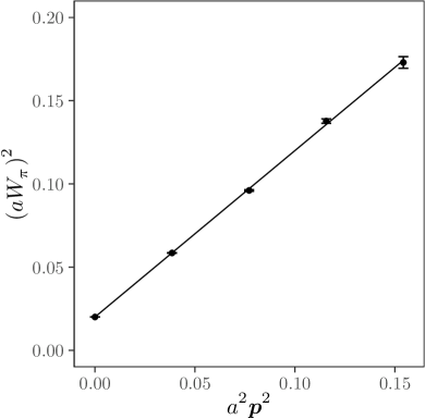
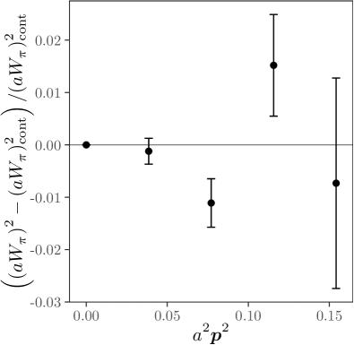
Figure 1: Dispersion relation of the pion for ensemble A40.32. Left: $W_{\pi}(\bm{p})^{2}$ as a function of $\bm{p}^{2}$, both in lattice units. The solid line represents the continuum dispersion relation. Right: relative difference of measured $W_{\pi}(\bm{p})^{2}$ and the corresponding prediction of the continuum dispersion relation.

4 Results

4.1 Pion Dispersion Relation

In order to extract the energy shift, we need the pion energy not only at rest but also in moving frames. As mentioned before, in order to reduce statistical uncertainties we are going to use the relativistic continuum dispersion relation

$$W_{\pi}^{2}(\bm{p})=M_{\mathup{{{\pi}}}}^{2}+\bm{p}^{2}$$ (32)

to compute $W_{\pi}(\bm{p})$ from the zero momentum pion mass value. As a check for the validity of this approach we have also computed $W_{\pi}(\bm{p})$ from two-point correlation functions with momentum.

In Figure 1 we compare the measured $W_{\pi}^{2}(\bm{p})$ with the prediction of Eq. (32) with $M_{\pi}^{2}$ at zero momentum as input exemplarily for the A40.32 ensemble. Good agreement within errors is observed up to $\bm{d}^{2}=4$. This makes us confident that using the dispersion relation is safe.

4.2 Energy Levels

One of the major uncertainties in our extraction of energy levels of multi-particle correlation functions is caused by thermal pollutions. For the case of two pions with maximal isospin the onset of thermal pollutions in Euclidean time in the correlators is clearly visible. However, due to the exponential deterioration of the signal-to-noise ratio, this is not the case for the correlation functions investigated here. This manifests itself also in the fact that there is no clear difference visible between principal correlators $\lambda(t,t_{0})$ derived from $\mathcal{C}(t,t_{0})$ or their weighted and shifted counterparts $\tilde{\lambda}(t,t_{0})$ derived from $\tilde{\mathcal{C}}(t,t_{0})$. Therefore, we perform the full analysis with and without weighting and shifting and include the difference as a systematic uncertainty in our error budget.

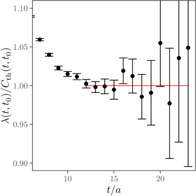
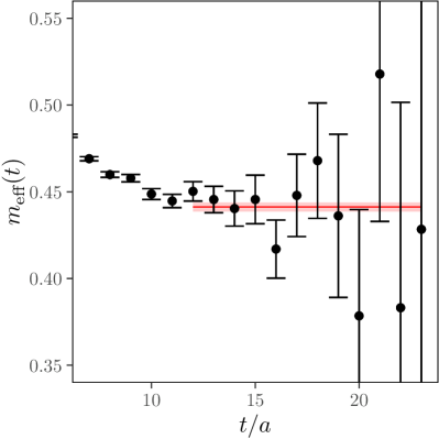
Figure 2: In the left panel we show $\lambda(t,t_{0})/C_{\mathrm{th}}(t,t_{0})$ as a function of $t/a$ for the ground state energy level in irrep $\mathrm{E}$. The reference time for the GEVP was set to $t_{0}/a=3$ and the ensemble is A40.32. The horizontal line indicates the fit range. In the right panel we show the effective mass as a function of $t/a$ and the fitted energy value with error band for reference.

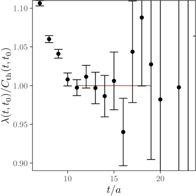
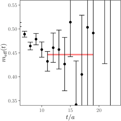
Figure 3: the same as Figure 2, but for weighted and shifted $\tilde{\lambda}$.

The other major uncertainty in extracting energy levels from lattice correlation functions stems from the choice of fit range. There have been approaches to make this choice more objective by performing a weighted average over many fit ranges, which works well for the case of single pions or two pions with maximal isospin. In contrast, for the case in question here, the $\rho$ channel, the weighted average turns out not to be useful.

Therefore, our procedure is the following: we perform the fitting to the principal correlator $\lambda(t,t_{0})$ (and $\tilde{\lambda}$) by surveying multiple fit ranges $[t_{\text{min}},t_{\text{max}}]$ and selecting a representative one. We enforce a plateau length of at least four points, which must be compatible within errors and have relative errors below 50%. Additionally we require no significant dependence on $t_{\text{max}}$ as this would be a consequence of residual thermal pollution. The dependence on $t_{\text{min}}$ is very pronounced when $t_{\text{min}}$ is in a region, where excited states are still relevant. We increase $t_{\text{min}}$ until this dependence vanishes. A $p$-value above $0.05$ was preferred to ascertain that the data in the chosen range are described by our fit. In the rare cases where multiple fit ranges gave competing and equally likely results, we chose an intermediate range. The influence of varying $t_{0}$ from $1$ to the onset of the plateau was checked and found to be negligible. Therefore, we chose $t_{0}=3$ on the coarser two and $t_{0}=4$ on the finest lattice spacing, corresponding to approximately $0.25\ \textrm{fm}$ in physical units. Finally, all other qualities being equal, we preferred larger $t_{\text{max}}$.

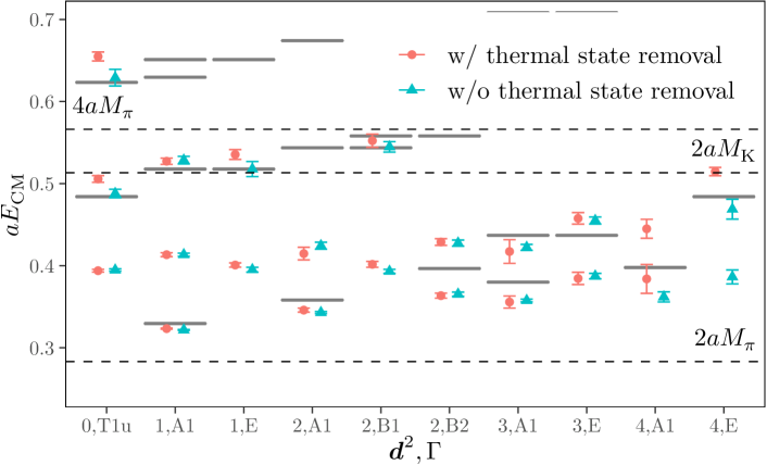
Figure 4: Example of all energy levels in lattice units for ensemble A40.32 for irrep $\Gamma$ and $\bm{p}_{\text{cm}}$ labeled by $\bm{d}^{2}$. The two kaon, two pion and four pion thresholds are indicated by the dashed horizontal lines. The shorter solid lines indicate the non-interacting energy levels in each irrep. The two colours and symbols distinguish the estimate of $E_{\mathrm{CM}}$ with and without thermal state removal.

In Figure 2 we show an example for the fit range chosen for ensemble A40.32 where $d^{2}=1$ and irrep $\Gamma=\textrm{E}$ without weighting and shifting. In the left panel, we show the ratio of principal correlator $\lambda(t,t_{0})$ and the single exponential fit model $\mathcal{C}_{\mathrm{th}}(t,t_{0})=\exp(-W(t-t_{0}))$. Compared to the effective mass, the ratio is more robust numerically. By definition the central value is $1$. In the right panel we show for illustration the result of the correlator fit as a red band along with the effective mass

$$m_{\text{eff}}(t)=\log\frac{\mathcal{C}(t)}{\mathcal{C}(t+1)}\,.$$

As mentioned above, the effects of thermal states are not visible here. The energy level was determined as $aW=0.4412(26)$.

In Figure 3 we show the same plots but this time with weighting and shifting. The size of error bars is increased compared to without weighting and shifting, which can be explained by the reduced correlation of neighbouring time slices. For very large $t$, points are not depicted because they were compatible with zero. For this reason, $t_{\text{max}}$ was chosen smaller compared to before. The fit model was modified as described in Eq. (25) and the calculation of the effective mass in the right panel was changed accordingly. The fit result increased by roughly one standard deviation to $aW=0.4463(23)$. Whether this results from the independent choice of a fit range or due to not visible but barely significant thermal states remains hard to decide. By including this difference as a systematic error we are confident that we keep control of both major sources of systematic uncertainties.

In Figure 4 we show all energy levels $aE_{\mathrm{CM}}$ for all irreps $\Gamma$ and boosts $\bm{d}^{2}$ exemplary for ensemble A40.32. The red circles are with weighting and shifting, the blue triangles without. The two kaon upper and two pion lower thresholds are indicated by the dashed horizontal lines. For all $\bm{d}^{2}$-value and irrep combinations, apart from two, we have two energy levels below the two kaon inelastic threshold.

Comparing energy levels with and without thermal state removal, we observe good agreement. Statistical uncertainties are in general larger with weighting and shifting.

4.3 Phase Shift Determination

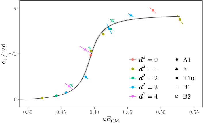
Figure 5: Phase shift $\delta_{1}$ as a function of $E_{\mathrm{CM}}$ in lattice units for ensemble A40.32. The solid line with error band represents the fit result of Eq. (26) to all the data w/ thermal state removal. Colours encode the different $\bm{d}^{2}$-values, while symbols distinguish the irreps.

In Figure 5 we show the phase shift $\delta_{1}$ as a function of the centre-of-mass energy $aE_{\mathrm{CM}}$ for ensemble A40.32. The two-parameter fit of Eq. (26) to our data is shown as a solid line with error band. Colours and symbols encode $\bm{d}^{2}$-values and irreps $\Gamma$, respectively. Error bars for the data points are slanted: $x$- and $y$-errors are added vectorially, i.e. the length of the slanted error bars is the sum of $x$- and $y$-error added in quadrature. Positive or negative slope of the slanted error bar indicates positive or negative correlation between $x$- and $y$-data. From Figure 5 one can, hence, deduce that $\delta_{1}$ is negatively correlated with $aE_{\mathrm{CM}}$. Note that for determining $\delta_{1}$ also $aM_{\pi}$ is needed. Here we use the finite volume estimate as argued in Ref. Romero-Lopez:2018rcb .

One also reads off from Figure 5 that our fit describes the data particularly well in the region where $\delta_{1}$ passes through $\pi/2$. Larger deviations can be observed for larger values of $\delta_{1}$, which significantly increase the $\chi^{2}$-values.

We have performed a list of variations of the fit to the phase shift data: a) the fits are being performed with and without (w and w/o) thermal state removal; b) we have performed fits by removing all points with $\bm{d}^{2}>k$ with $k=3,2,1$. While b) merely influences the statistical uncertainty, a) leads to up to $4$ standard deviations differences in the fit parameters, in particular in $M_{\rho}$. However, it is not clear whether approaches w/o or w/ thermal state removal are systematically cleaner: in the former case we might be plagued with thermal state pollutions, while in the latter case the fit range might be chosen incorrectly due to noise.

Therefore, we decided to use the weighted mean over results w/o and w/ thermal state removal. In addition we include the difference $\Delta Q_{Y}$ between the weighted mean and w/o and w/ thermal state removal into the error by rescaling the bootstrap distribution with a factor Helmes:2018nug

$$s\ =\ \sqrt{\frac{(\Delta x)^{2}+\sum_{Y}(\Delta Q_{Y})^{2}}{(\Delta x)^{2}}}\,.$$ (33)

Here, $\Delta x$ is the statistical uncertainty of the weighted mean and $Y\in\{\mathrm{w/o},\mathrm{w/}\}$.

All results for $M_{\rho}$ and $g_{\rho\pi\pi}$ determined by this procedure w/ and w/o thermal state removal are compiled in Table 4. The width $\Gamma_{\rho}$ computed via Eq. (27) is tabulated in Table 5. In the latter table we also give the reduced $\chi^{2}$-values of the Breit-Wigner fits and the values for the (charged) pion mass in lattice units $aM_{\pi}$.

Ensemble	$aM_{\rho}^{\mathrm{w/o}}$	$aM_{\rho}^{\mathrm{w/}}$	$aM_{\rho}^{\mathrm{av}}$	$g_{\rho\pi\pi}^{\mathrm{w/o}}$	$g_{\rho\pi\pi}^{\mathrm{w/}}$	$g_{\rho\pi\pi}^{\mathrm{av}}$
A30.32	0.3906(11)	0.3968(15)	0.3929(32)	6.0(2)	5.8(2)	6.0(2)
A40.24	0.4010(15)	0.4084(14)	0.4051(38)	5.7(1)	4.9(2)	5.4(4)
A40.32	0.3957(12)	0.3971(13)	0.3964(11)	5.7(1)	5.5(2)	5.6(1)
A60.24	0.4134(12)	0.4170(12)	0.4153(20)	5.4(1)	5.4(1)	5.4(1)
A80.24	0.4265(11)	0.4314(14)	0.4282(26)	5.3(1)	5.0(3)	5.2(2)
A100.24	0.4512(11)	0.4521(12)	0.4516(09)	4.7(2)	5.0(2)	4.9(2)
B25.32	0.3527(30)	0.3608(40)	0.3556(47)	6.3(3)	5.9(6)	6.2(4)
B35.32	0.3554(17)	0.3582(17)	0.3568(18)	6.3(2)	5.4(3)	6.0(5)
B35.48	0.3617(15)	0.3609(26)	0.3615(13)	5.8(2)	6.6(5)	6.0(4)
B55.32	0.3709(09)	0.3739(09)	0.3722(16)	5.6(1)	6.1(1)	5.8(3)
D15.48	0.2751(35)	-	0.2751(35)	6.5(7)	-	6.5(7)
D30.48	0.2747(16)	0.2926(22)	0.2811(91)	5.3(4)	5.1(5)	5.2(3)
D45.32	0.2866(09)	0.2948(14)	0.2890(42)	5.8(2)	4.6(5)	5.6(6)

Table 4: $\rho$ mass $aM_{\rho}$ and coupling $g_{\rho\pi\pi}$ for all ensembles w/ and w/o thermal state removal and the weighted average including the systematic uncertainty as explained in the text.

Ensemble	$aM_{\pi}$	$K_{M_{\pi}}$	$a\Gamma_{\rho}^{\mathrm{w/o}}$	$a\Gamma_{\rho}^{\mathrm{w/}}$	$a\Gamma_{\rho}^{\mathrm{av}}$	$\chi^{2}_{\mathrm{w/o}}$	$\chi^{2}_{\mathrm{w/}}$
A30.32	0.12392(13)	1.0081(52)	0.0435(23)	0.0427(30)	0.0432(19)	2.66	2.79
A40.24	0.14154(12)	1.0206(95)	0.0312(14)	0.0243(15)	0.0279(36)	1.77	1.43
A40.32	0.14429(20)	1.0039(28)	0.0287(15)	0.0271(18)	0.0280(14)	1.81	1.49
A60.24	0.17314(19)	1.0099(49)	0.0133(07)	0.0139(07)	0.0136(06)	2.53	1.11
A80.24	0.19909(17)	1.0057(29)	0.0036(03)	0.0040(05)	0.0037(03)	1.72	0.54
A100.24	0.22236(23)	1.0037(19)	0.0003(01)	0.0004(01)	0.0004(01)	0.41	8.14
B25.32	0.10850(32)	1.0136(60)	0.0454(50)	0.0427(89)	0.0447(46)	1.05	0.56
B35.32	0.12380(10)	1.0069(32)	0.0340(20)	0.0260(26)	0.0309(43)	0.97	0.90
B35.48	0.12486(14)	-	0.0316(24)	0.0397(56)	0.0328(46)	1.35	0.88
B55.32	0.15551(12)	1.0027(14)	0.0123(05)	0.0156(07)	0.0136(17)	1.30	0.93
D15.48	0.07067(15)	1.0081(22)	0.0491(114)	-	0.0491(114)	0.68	-
D30.48	0.09754(14)	1.0021(07)	0.0179(25)	0.0206(40)	0.0187(25)	1.03	2.79
D45.32	0.12046(19)	1.0047(14)	0.0102(06)	0.0079(15)	0.0098(13)	1.17	0.93

Table 5: We give $aM_{\pi}$, the finite size correction factor $K_{M_{\pi}}$, the $\rho$ width $a\Gamma_{\rho}$ computed from $aM_{\rho}$ and $g_{\rho\pi\pi}$ using Eq. (27) w/ and w/o thermal state removal, and the weighted average as explained in the text. In addition we give the reduced $\chi^{2}$-values of the corresponding fits to the phase shift data.

We have two groups of ensembles with all identical parameters apart from the volume. These are ensembles A40.24 and A40.32 as well as B35.32 and B35.48, which we can use to investigate residual finite volume effects in our results for $M_{\rho}$ and $\Gamma_{\rho}$.

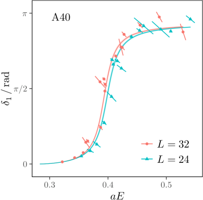
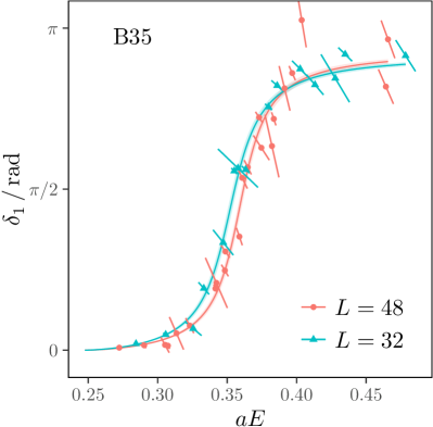
Figure 6: We show the phase-shift $\delta_{1}$ as a function of $E_{\mathrm{CM}}$ in lattice units. Left we compare A40.24 (blue) with A40.32 (red) and right B35.48 (red) with B35.32 (blue). The lines with error bars represent the corresponding fits with Eq. (26) to the data.

In Figure 6 we compare in the left panel the phase shift points for A40.24 (blue) with the ones for A40.32 (red), in the right panel B35.48 (red) with B35.32 (blue). Even though the Breit-Wigner fits happen to result in slightly different values for the resonance parameters, deviations are below the $2\sigma$ level and do not show a systematic ordering with volume, see Table 4 and Table 5.

Thus, the weighted average with error including the systematic uncertainty from thermal state removal should also safely include residual effects from finite volume.

There are a few ensembles where the Breit-Wigner type fits to the phase shift points are problematic. On the one hand this is the case for ensemble with the heaviest pion mass A100.24. The width approaches zero, which leaves the fits little freedom; a fact reflected by the untrustworthy $\chi^{2}$.

On the other hand, unfortunately the fit on D15.48, our most chiral ensemble, is difficult, however, for different reasons. For D15.48 statistical uncertainties on the energy levels are quite large. As a consequence, the Breit-Wigner fit for the case w/ thermal state removal is not converging. The fit for the case w/o thermal state removal gives large uncertainties. Combined with the rather low lying inelastic threshold at $2M_{K}$, we do not consider this ensemble as trustworthy for this calculation.

4.4 Chiral extrapolation

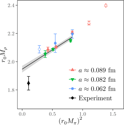
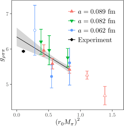
Figure 7: In the left panel we show $r_{0}M_{\rho}^{\mathrm{av}}$ as a function of $(r_{0}M_{\pi})^{2}$. Open symbols are not included in the fit. In the right panel $g_{\rho\pi\pi}^{\mathrm{av}}$ is shown also as a function of $(r_{0}M_{\pi})^{2}$. The lines with error bands represent independent fits to the data.

We first consider $M_{\rho}$ and $g_{\rho\pi\pi}$. In the left panel of Figure 7 we show $r_{0}M_{\rho}^{\mathrm{av}}$, in the right one $g_{\rho\pi\pi}^{\mathrm{av}}$, both as a function of $(r_{0}M_{\pi})^{2}$. Note that the error on $r_{0}/a$ is not included in the plot, because it is 100% correlated for all data points of the same $\beta$-value. Colours and symbols encode the three lattice spacing values. The black diamonds represent the corresponding experimental values. The first observation is that lattice artefacts are not resolvable given our current level of statistical uncertainty. Overall, $M_{\rho}$ appears to show a rather linear dependence on $M_{\pi}^{2}$, a bit less so $g_{\rho\pi\pi}$. The values for $aM_{\pi}$ can be found in Table 5. For the following extrapolations we correct $aM_{\pi}$ for finite size effects by applying a correction factor $K_{M_{\pi}}$ computed in Ref. Carrasco:2014cwa , which can also be found in Table 5.

Next we have tried to fit the pion mass dependence of $M_{\rho}^{\mathrm{av}}$ and $g_{\rho\pi\pi}^{\mathrm{av}}$ combining Eqs. (28) and (29) up to the order $M_{\pi}^{3}$. However, such a fit did not result in convincing results. Even though the chiral log in $g_{\rho\pi\pi}^{\mathrm{av}}$ stemming from $f_{\pi}$ somewhat compensates the term $c_{1}M_{\pi}^{2}$, a satisfactory description of the data for both the mass and the coupling could not be achieved.

Therefore, we show in Figure 7 independent linear extrapolations for both $M_{\rho}$ and $g_{\rho\pi\pi}$ in $M_{\pi}^{2}$. As visible, the two extrapolations overestimate both the $\rho$ mass and the coupling at the physical point compared to experiment.

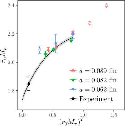
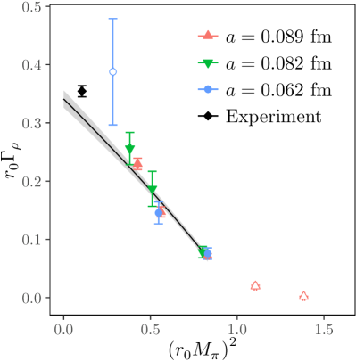
Figure 8: Chiral extrapolation of $M_{\rho}$ and $\Gamma_{\rho}$ as a function of $M_{\pi}^{2}$, all in units of the Sommer parameter $r_{0}$. The lattice spacing is colour and symbol coded, the experimental values are shown as black diamonds. The lines with error bands represent combined fits according to Eq. (34) to the data of $M_{\rho}$ and $\Gamma_{\rho}$. Data points with open symbols are not included in the fit.

We now turn to combined fits of mass and width using Eq. (31) for the complex valued variable $Z$. As described in section 3, we extrapolate $M_{\rho}$ and $\Gamma_{\rho}$ to the physical point combined in $r_{0}^{2}Z=r_{0}^{2}(M_{\rho}+\mathrm{i}\Gamma_{\rho}/2)^{2}$. As we also mentioned already, the error analysis for this fit is performed using the parametric bootstrap procedure maintaining the correlation among $M_{\rho}$, $\Gamma_{\rho}$ and $M_{\pi}$. We use $1500$ bootstrap samples and the values for $r_{0}/a$ for the different lattice spacings were resampled from the values compiled in Table 2.

The actual fit function reads

$$\begin{split}a^{2}Z&=p_{r_{0}/a}^{-2}\left((p_{1}+ip_{2})+p_{3}\left(p_{r_{0}/a}aM_{\mathup{{{\pi}}}}\right)^{2}\right.\\ &\quad-p_{4}\sqrt{p_{1}+ip_{2}}\left(p_{r_{0}/a}aM_{\mathup{{{\pi}}}}\right)^{3}\\ &\left.\quad+(p_{5}+ip_{6})\ p_{r_{0}/a}^{-2}\right)\,.\end{split}$$ (34)

The fit parameters are the following: $p_{1}$ and $p_{2}$ represent the real and imaginary parts of $r_{0}^{2}Z_{\chi}$ and $p_{3}$ represents $C_{\chi}$, furthermore $p_{4}\equiv g^{2}_{\omega\rho\pi}/(24\pi r_{0}^{2})$ and $p_{5}$ and $p_{6}$ parametrise the real and imaginary part of the $a^{2}$ lattice artefacts. $p_{r_{0}/a}$ is one fit parameter per lattice spacing value for $r_{0}/a$ accompanied by a corresponding prior $P_{r_{0}/a}$. Thus, we have in total $6$ real-valued free fit parameters.

In the fit we include only the ensembles with the largest volume per pion mass value, i.e. A40.24 and B35.32 are not included in the fit. We do not include ensemble D15.48 in the fit, for reasons mentioned above. Moreover, we include only data points with $M_{\pi}\leq 420\ \mathrm{MeV}$, which excludes ensembles A80.24 and A100.24.

The best fit parameters can be found in Table 6 together with the reduced $\chi^{2}$-value. We give the best fit parameters for fits with and without lattice artefacts included. Clearly, $p_{5}$ and $p_{6}$, which parametrise the $a^{2}$ effects in $Z$ are compatible with zero. Also, the remaining parameters do not change significantly with and without $a^{2}$ artefact included in the fit.

Parameter	incl. $a^{2}$	excl. $a^{2}$
$p_{1}$	3.14(28)	2.99(07)
$p_{2}$	-0.631(61)	-0.592(26)
$p_{3}$	4.75(24)	4.79(08)
$p_{4}$	0.936(80)	0.991(34)
$p_{5}$	-5(10)	-
$p_{6}$	1.3(1.8)	-
$\chi^{2}/\text{d.o.f.}$	2.35	2.00

Table 6: Best fit parameters of the combined chiral fit in terms of $Z$ with and without lattice artefacts included in the fit.

The $\chi^{2}$-values for these fits are all a bit too large, indicating a tension in the data in particular between $M_{\rho}$ and $\Gamma_{\rho}$. It basically is a consequence of the invisible curvature in the data for $M_{\rho}$.

The result of the fit can be seen in Figure 8, where we show in the left panel $r_{0}M_{\rho}$ and in the right panel $r_{0}\Gamma_{\rho}$ both as functions of $(r_{0}M_{\pi})^{2}$. Note that the error on $r_{0}/a$ is not included in the plot, because it is 100% correlated for all data points of the same $\beta$-value. The best fit to the data is indicated by the solid lines with error bands. Data points with open symbols are excluded from the fit. The fit range is indicated by the extent of the solid lines. The experimental values are included in both plots as black diamonds, but not included in the fit.

Our final result for $M_{\rho}$ and $\Gamma_{\rho}$ taken from the fit without a $a^{2}$ effects included reads

$$M_{\rho}\ =\ 769(19)\ \mathrm{MeV}\,,\qquad\Gamma_{\rho}\ =\ 129(7)\ \mathrm{MeV}\,,$$ (35)

corresponding to

$$g_{\rho\pi\pi}\ =\ 5.5(1)\,.$$ (36)

In addition we find

$$\begin{split}M_{\rho}^{0}\ &=\ 723(20)\ \mathrm{MeV}\,,\\ \Gamma_{\rho}^{0}\ &=\ 142(7)\ \mathrm{MeV}\,,\\ |g_{\omega\rho\pi}|\ &=\ 20.8(7)\ \mathrm{GeV}^{-1}\\ \end{split}$$ (37)

from our chiral and continuum fits. The correlation coefficients for the fit parameters can be found in appendix C.

5 Discussion

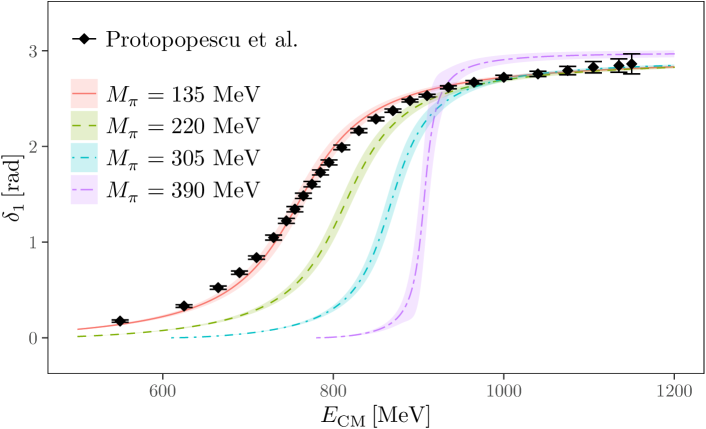
Figure 9: Comparison of experimental phase shift data from Ref. Protopopescu:1973sh to the phase shift curve extracted from our final results for $M_{\rho}$ and $\Gamma_{\rho}$ shown as red solid line. For illustration purposes we also show the phase shift curve in a world with $M_{\pi}=220\ \mathrm{MeV}$ as green dashed line, with $M_{\pi}=305\ \mathrm{MeV}$ as blue dot-dashed line and with $390\ \mathrm{MeV}$ as a purple two-dashed line.

In the previous section we have performed different chiral and continuum extrapolations for our data. First, there are independent linear fits of $M_{\rho}$ and $g_{\rho\pi\pi}$ as a function of $M_{\pi}^{2}$. Second, we have performed combined fits in terms of $Z$ as function of $M_{\pi}$ including terms up to order $M_{\pi}^{3}$ with and without including lattice artefacts. While the two linear fits certainly provide a good description of the data for $M_{\rho}$ and $g_{\rho\pi\pi}$ separately, we decided to quote the results from the combined fit as our final result. The reason is that in the corresponding effective field theory the complex pole is treated consistently, which we consider as theoretically more sound.

The final result for $M_{\rho}$ and $\Gamma_{\rho}$ we quote in Eq. (35) can be compared to the corresponding PDG values Tanabashi:2018oca for mass and full width

$$M_{\rho}^{\mathrm{exp}}\ =\ 775.26(25)\ \mathrm{MeV}\,,\qquad\Gamma_{\rho}^{\mathrm{exp}}\ =\ 149.1(8)\ \mathrm{MeV}\,.$$

Note that these also correspond to Breit-Wigner parameters determined experimentally from $e^{+}e^{-}$ reactions. The deviation to other reactions can be of the order of $10\ \mathrm{MeV}$. We observe rather good agreement for $M_{\rho}$, while our value for the width is slightly too low. This is also visible in Figure 9, where we plot the experimental phase shifts from Ref. Protopopescu:1973sh and compare them to the phase shift curve we obtain using the final values from Eq. (35) and then again assuming the Breit-Wigner form from Eq. (26).

However, this good agreement should be taken with caution. First of all our extrapolation form for $M_{\rho}$ and $\Gamma_{\rho}$ is not model independent. This is in particular important, because the curvature needed to obtain an $M_{\rho}$-value close to the experimental one comes from constrains due to $\Gamma_{\rho}$. This, as discussed earlier, manifests itself also in a bit too large $\chi^{2}$-values in the chiral and continuum fits. Moreover, the ensemble with the lightest pion mass included in the fit is B35.48 with a pion mass of about $300\ \mathrm{MeV}$. Thus, the extrapolation to the physical point is quite long. In addition we have assumed that we can perform a Breit-Wigner type fit to all the phase shift data, which is an approximation. This might also be the reason for the too low value of $\Gamma_{\rho}$ compared to experiment. We are currently working on an alternative extrapolation using the inverse amplitude method which might allow us to perform the chiral extrapolation even more reliably Truong:1991gv ; Dobado:1992ha ; Dobado:1996ps ; GomezNicola:2007qj ; Niehus:2019nkl . Our fitted value for $g_{\omega\rho\pi}$ Eq. (37) is in the right ballpark, when compared to the numbers given in Refs. Djukanovic:2009zn ; Djukanovic:2010id , where $16\ \mathrm{GeV}^{-1}$ is quoted. From Refs. Meissner:1987ge ; Kaiser:1990yf one finds $g_{\omega\rho\pi}=\pm 20.7\ \mathrm{GeV}^{-1}$ in very good agreement with our value.

Finally, our determinations of mass and width rest on the assumption that all partial waves apart from $\ell=1$ are negligible. This assumption is supported by previous lattice investigations of the $\rho$ meson, but has not been checked by us yet.

On the other hand, our results for $M_{\rho}$ and $\Gamma_{\rho}$ make a combined extrapolation to the physical point and to the continuum limit feasible for the first time. However, since we find lattice artefacts to be statistically insignificant, our final result is based on a chiral extrapolation assuming no lattice artefacts. We have different volumes available with otherwise fixed parameters, which allow us to argue that residual finite volume effects are not a dominant source of uncertainty in our results.

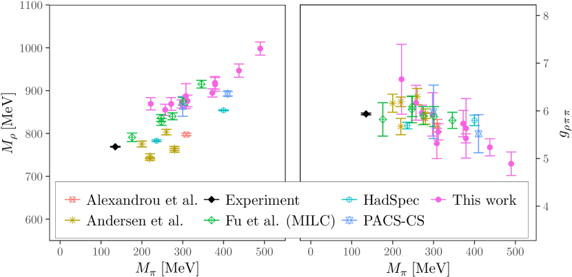
Figure 10: Comparison of lattice results for $M_{\rho}$ (left) and $g_{\rho\pi\pi}$ (right) as a function of $M_{\pi}$. We compare with all available results that had a dynamic strange quark: Alexandrou et al. Alexandrou:2017mpi , Andersen et al. Andersen:2018mau , Fu et al. Fu:2016itp , HadSpec Dudek:2012xn ; Wilson:2015dqa , PACS-CS Aoki:2011yj as well as the experimental value Tanabashi:2018oca .

In Figure 10 we compare results for $M_{\rho}$ and $g_{\rho\pi\pi}$ from various lattice collaborations with $N_{f}=2+1$ or $N_{f}=2+1+1$ dynamical quark flavours. We observe that there are probably lattice artefacts in some of the results for $M_{\rho}$, in particular in the results from Andersen et al. Andersen:2018mau and from the Hadron Spectrum Collaboration Dudek:2012xn . For $g_{\rho\pi\pi}$ uncertainties are in general larger and within these large uncertainties the agreement among different lattice collaborations is reasonable.

However, leaving aside lattice artefacts, one could be tempted to conclude from Figure 10 that $M_{\rho}$ is rather linear in $M_{\pi}$, very similar to what is observed for the nucleon mass Walker-Loud:2014iea . In fact one finds $M_{\rho}=680\ \mathrm{MeV}+0.6M_{\pi}$ to a good approximation by fitting only the data by Fu and Wang Fu:2016itp together with our data, which represents yet another version of the “ruler” plot. From an effective field theory point of view this cannot be the correct pion mass dependence and future results will hopefully shed light on this puzzle.

We can also compare to the results of Ref. Giusti:2018mdh , where $M_{\rho}$ and $g_{\rho\pi\pi}$ have been determined on the same ETMC ensembles we used, however, using the inverse Lüscher method based only on the vector current based on a parametrisation of the pion form factor. Their continuum extrapolated values for $M_{\rho}$ and $g_{\rho\pi\pi}$ at the physical point are consistent with ours.

6 Summary

We have presented an investigation of the $\rho$-meson properties using lattice QCD with $N_{f}=2+1+1$ Wilson twisted mass quarks at maximal twist. With three values of the lattice spacing and a range of pion mass values we could perform chiral and continuum extrapolations of $\rho$-meson mass $M_{\rho}$ and width $\Gamma_{\rho}$ with better control than previously possible. The latter two quantities have been determined on our ensembles using a Breit-Wigner type fit to phase shift data assuming that partial waves with $\ell\geq 3$ are negligible.

The phase shift curves have been determined applying Lüscher’s method using moving frames up to $\bm{d}^{2}=4$ and all available lattice irreducible representations. Our final result reads

$$\begin{split}M_{\rho}\ &=\ 769(19)\ \mathrm{MeV}\,,\\ g_{\rho\pi\pi}\ &=\ 5.5(1)\,,\\ \Gamma_{\rho}\ &=\ 129(7)\ \mathrm{MeV}\,,\\ \end{split}$$

which is determined from a combined continuum and chiral extrapolation of $M_{\rho}$ and $\Gamma_{\rho}$. Systematic errors from thermal state pollutions, the chiral and the continuum extrapolation should be covered by the error we quote. $M_{\rho}$ is very close to its experimental value, the width is about two sigma too low. The agreement of our data for $M_{\rho}$ with previously published lattice results is satisfactory.

It is clear that more work is needed to better estimate the width, which likely suffers from e.g. the use of a Breit-Wigner type fit to the phase shift data. Therefore, we are currently working on using the inverse amplitude method to directly describe the pion mass dependence of the phase shift curves Niehus:2019nkl , see also Ref. Hu:2017wli . This should alleviate systematic uncertainties in our current analysis.

Appendix A Operator construction

One side effect of the restriction to finite volumes in a lattice calculation is, that the symmetry group of rotoflections (rotations and space inversions) is reduced to a finite subset. In sections 3.1 and 3.3, the consequences of this explicit symmetry breaking were encapsulated in a set of subduction coefficients. Here we illustrate our derivation of subduction coefficients as well as the chosen conventions for a single and two pions.

Let $\ket{l,m}$ be a basis vector in the spherical basis transforming according to the angular momentum-$l$ representation of $\mathrm{SO}(3)$ and $m$ denote the magnetic quantum number. For a given rotation $R$ and basis vectors $\ket{l,m}$, the representation matrix elements are given by

$$D^{l}_{m,m^{\prime}}(R) =\matrixelement{l,m}{\hat{R}}{l,m^{\prime}}\,,$$ (38)

where $\hat{R}$ denotes the action of $R$ on the Hilbert space of wave functions.

Let $\mathit{G}$ be the (finite) symmetry group of the discretised geometry. As already explained in Eq. (9), $D^{l}$ is not necessarily irreducible over $\mathit{G}$ and it may decompose into multiple irreducible representations $\Gamma$ of $\mathit{G}$. Then

$$\hat{P}_{\alpha\beta}^{\Gamma,l} =\frac{\mathrm{dim}(\Gamma)}{\absolutevalue{\mathit{G}}}\sum\limits_{g\in\mathit{G}}D^{\Gamma}(R_{g})^{*}_{\alpha\beta}\hat{R}_{g}$$ (39)

defines a projector, where $D^{\Gamma}$ denote the irreducible representation matrices and $\alpha,\beta\,\in\,\left\{1,\ldots,\mathrm{dim}(\Gamma)\right\}$ are arbitrary but fixed. We refrain from discussing the modifications for non-trivial multiplicities. We use the Schönflies notation and follow the conventions for $D^{\Gamma}$ used in crystallography altmann1994point , conveniently implemented in Maple rykhlinskaya2005generation .

$\bm{d}^{2}$	$\mathrm{LG}(\bm{p}_{\text{cm}})$	$\Gamma$
$0$	$\mathrm{O}_{\text{h}}$	$\mathrm{T{1u}}$
$1$	$\mathrm{C}_{\text{4v}}$	$\mathrm{A1}\oplus\mathrm{E}$
$2$	$\mathrm{C}_{\text{2v}}$	$\mathrm{A1}\oplus\mathrm{B1}\oplus\mathrm{B2}$
$3$	$\mathrm{C}_{\text{3v}}$	$\mathrm{A1}\oplus\mathrm{E}$
$4$	$\mathrm{C}_{\text{4v}}$	$\mathrm{A1}\oplus\mathrm{E}$

Table 7: Little groups and decomposition of angular momentum 1 for all momentum sectors $\bm{d}^{2}$ used in this work. The groups are isomorphic for each representative of a sector. Therefore, the direction of $\bm{p}_{\text{cm}}$ is arbitrary here.

At rest, the symmetry group is the octahedral group $\mathrm{O}_{\text{h}}$. Choosing a non-zero CM-momentum $\bm{p}_{\text{cm}}$ further reduces the relevant symmetry group to the “little group”

$$\mathrm{LG}(\bm{p}_{\text{cm}})\equiv\{g\in\mathrm{O}_{\text{h}},\hat{R}_{g}\ \bm{p}_{\text{cm}}=\bm{p}_{\text{cm}}\}\,,$$ (40)

which leaves $\bm{p}_{\text{cm}}$ invariant. The relevant little groups are listed in Table 7.

A.1 One-meson operator

Let $\mathcal{O}_{l}^{m\dagger}(\bm{p}_{\text{cm}})$ be an operator that creates a meson state $\ket{\bm{p}_{\text{cm}};l,m}$ with momentum $\bm{p}_{\text{cm}}$ and total (integral) angular momentum $l$ with projection $m$. By applying $\hat{P}^{\Gamma,l}$, this operator is projected to an operator

$$\mathcal{O}_{\Gamma}^{\alpha\dagger}(\bm{p}_{\text{cm}}) =\sum_{\beta}\phi_{\beta}\sum_{m}\phi_{m}\hat{P}_{\alpha\beta}^{\Gamma,l}\,\mathcal{O}_{l}^{m\dagger}(\bm{p}_{\text{cm}})$$

$$=\sum_{\beta}\phi_{\beta}\sum\limits_{m,m^{\prime}}\phi_{m}\frac{\mathrm{dim}(\Gamma)}{\absolutevalue{\mathit{G}}}$$

$$\times\sum\limits_{g\in\mathrm{LG}(\bm{p}_{\text{cm}})}D^{\Gamma}(R_{g})^{*}_{\alpha\beta}\,D^{l}_{m^{\prime},m}(R_{g})\mathcal{O}_{l}^{m^{\prime}\dagger}(\bm{p}_{\text{cm}})\,,$$ (41)

which creates a single meson basis state $\ket{\bm{p}_{\text{cm}};\Gamma,\alpha}$ of $\mathrm{LG}(\bm{p}_{\text{cm}})$.

Here it becomes apparent, why $\alpha$ are called “rows”. The row index of the matrix $D^{\Gamma}$ also labels the basis vectors of $\Gamma$. Correspondingly we will refer to $\beta$ as the “column” of the representation. $\phi_{m}$ and $\phi_{\beta}$ are phases which are chosen such that the set $\ket{\bm{p}_{\text{cm}};\Gamma,\alpha}$ become orthonormal. In the following we suppress the dependence on $\beta$ and $\phi$. We denote the coefficients with fixed phases by the “subduction coefficient” $s^{\Gamma}_{l}$ and from Eq. (41) obtain the result

$$\mathcal{O}_{\Gamma}^{\alpha\dagger}(\bm{p}_{\text{cm}})=\sum\limits_{m^{\prime}}s^{\Gamma,\alpha}_{l,m^{\prime}}\,\mathcal{O}_{l}^{m^{\prime}\dagger}(\bm{p}_{\text{cm}})\,.$$ (42)

Applying the creation operators on the left and right side to a vacuum state yields Eq. (10) for the subduction of basis states. Note that the projection only acts in the space of total angular momentum. The linear momentum $\bm{p}$ is unaffected by the procedure.

A.2 Two-pion operators

$\bm{d}$	$\Gamma$	$\bm{p}_{1}\otimes\bm{p}_{2}$
$(0,0,0)$	$\mathrm{T1u}$	$(0,0,1)\otimes(0,0,-1)$, $(1,0,1)\otimes(-1,0,-1)$
$(0,0,1)$	$\mathrm{A1}$	$(0,0,1)\otimes(0,0,0)$, $(0,0,2)\otimes(0,0,-1)$, $(1,0,1)\otimes(-1,0,0)$, $(1,1,1)\otimes(-1,-1,0)$
$(0,0,1)$	$\mathrm{E}$	$(0,1,1)\otimes(0,-1,0)$, $(1,1,1)\otimes(-1,-1,0)$
$(1,1,0)$	$\mathrm{A1}$	$(1,1,0)\otimes(0,0,0)$, $(1,1,1)\otimes(0,0,-1)$, $(1,-1,0)\otimes(0,2,0)$
$(1,1,0)$	$\mathrm{B1}$	$(1,1,1)\otimes(0,0,-1)$, $(1,0,1)\otimes(0,1,-1)$
$(1,1,0)$	$\mathrm{B2}$	$(1,0,0)\otimes(0,1,0)$, $(1,0,1)\otimes(0,1,-1)$, $(2,0,0)\otimes(-1,1,0)$
$(1,1,1)$	$\mathrm{A1}$	$(1,1,1)\otimes(0,0,0)$, $(1,0,1)\otimes(0,1,0)$, $(2,0,0)\otimes(-1,1,1)$
$(1,1,1)$	$\mathrm{E}$	$(1,0,1)\otimes(0,1,0)$, $(1,-1,1)\otimes(0,2,0)$
$(0,0,2)$	$\mathrm{A1}$	$(0,0,2)\otimes(0,0,0)$
$(0,0,2)$	$\mathrm{E}$	$(0,1,1)\otimes(0,-1,1)$

Table 8: Momentum combinations $\bm{p}_{1}\otimes\bm{p}_{2}$ used in Eq. (43). We only give one representative CM momentum $\bm{p}_{\text{cm}}=2\pi\bm{d}/L$ for each momentum sector. The other directions may be generated by a global rotation. The momentum combinations depend on the irrep $\Gamma$ because not all combinations couple to all irreps.

To subduce the two-pion operators with individual 3-momenta $\bm{p}_{1},\,\bm{p}_{2}$ and $\bm{p}_{\text{cm}}=\bm{p}_{1}+\bm{p}_{2}$ into the irreducible representations of the residual lattice rotation symmetry group $\mathrm{LG}(\bm{p}_{\text{cm}})$ we start from the product operator $\mathup{{{\pi}}^{\scriptstyle{+}}}(\bm{x}_{1})\,\mathup{{{\pi}}^{\scriptstyle{-}}}(\bm{x}_{2})$. Then our group projection formula reads Feng:2010es

$$\begin{split}{\mathcal{O}_{\mathup{{{\pi}}}\mathup{{{\pi}}}}}^{\alpha\dagger}_{\Gamma\bm{q}}(\bm{p}_{\text{cm}})\quad&=\frac{\dim\left(\Gamma\right)}{|\mathrm{LG}(\bm{p}_{\text{cm}})|}\\ &\times\sum\limits_{\beta}\phi_{\beta}\,\sum_{g\in\mathrm{LG}(\bm{p}_{\text{cm}})}\sum_{\bm{x}_{1},\bm{x}_{2}}\\ &\times\mathrm{e}^{i(\bm{x}_{1}\cdot(\frac{1}{2}\bm{p}_{\text{cm}}+\hat{R}_{g}\bm{q})+\bm{x}_{2}\cdot(\frac{1}{2}\bm{p}_{\text{cm}}-\hat{R}_{g}\bm{q}))}\,\\ &\times D^{\Gamma}(R_{g})_{\alpha\beta}^{*}\,\mathcal{O}^{\dagger}_{\mathup{{{\pi}}^{\scriptstyle{+}}}}(\bm{x}_{1})\,\mathcal{O}^{\dagger}_{\mathup{{{\pi}}^{\scriptstyle{-}}}}(\bm{x}_{2})\,,\\ \end{split}$$ (43)

where $2\bm{q}=\bm{p}_{1}-\bm{p}_{2}$ and $\alpha=1,\cdots,\dim\left(\Gamma\right)$. The vector $\phi=\left(\phi_{1},\cdots,\phi_{\dim\left(\Gamma\right)}\right)$ characterises again our choice of phase and normalisation for the irreducible operator multiplet.

Two-pion operators in the same reference frame $\bm{p}_{\text{cm}}$ but with different relative momenta $\bm{q}\neq\bm{q}^{\prime}$, which are related by an element of $\mathrm{LG}(\bm{p}_{\text{cm}})$, $\hat{R}_{g}\bm{q}=\bm{q^{\prime}}$ for some $g\in\mathrm{LG}(\bm{p}_{\text{cm}})$, lead to linearly dependent operators under the projection Eq. 43. Therefore, we only use certain momentum combinations $\bm{p}_{1}\otimes\bm{p}_{2}$. In Tab. 8 we list one representative combination for each momentum sector. The two-pion operators for unlisted moving frames $\bm{p}_{\text{cm}}^{\prime}$ with $|\bm{p}_{\text{cm}}|=|\bm{p}_{\text{cm}}^{\prime}|$ are constructed by a global rotation for which $\hat{R}_{\tilde{g}}\bm{p}_{\text{cm}}=\bm{p}_{\text{cm}}^{\prime}$.

The method we describe here can be understood as an extension of the projection method of Ref. Prelovsek:2016iyo for arbitrary moving frames.

Appendix B Analysis Details

In this appendix we give the details on our analysis to estimate the extrapolated values for $M_{\rho}$ and $\Gamma_{\rho}$ starting from energy levels $aE_{\mathrm{CM}}$ and $aM_{\pi}$.

On a per ensemble basis we use the various interacting energy levels $aE_{\mathrm{CM}}$ together with the values of $aM_{\pi}$ to determine phase shift values $\delta_{1}(E_{\mathrm{CM}})$. For the reasons explained above we use in this step the jack-knife procedure to estimate the variance-covariance matrix for all $aE_{\mathrm{CM}}$, $\delta_{1}$ and $M_{\pi}$ using the standard jack-knife estimators. In particular, the Lüscher function is evaluated on the jack-knife samples.

Since with jack-knife there are not neccessarily identical numbers of replicates for all ensembles, we now use parametric bootstrap to resample the distributions with $1500$ bootstrap replicates on each ensemble. With all the mean values and the variance-covariance matrix as input we draw random samples from a corresponding multivariate Gaussian distribution. The such generated bootstrap replicates fully reproduce the input variance-covariance matrix.

Generating multi-variate Gaussian random variables $Y$ with a given symmetric, positive definite covariance matrix $C$ from independent standard normal random variables $X$ can be performed as follows:

$$\begin{split}Y=\sqrt{C}X\quad&\Rightarrow\\ \quad\mathrm{Cov}(Y,Y)\ &=\ \langle Y\cdot Y^{t}\rangle=\sqrt{C}\,\langle X\cdot X^{t}\,\rangle\,\sqrt{C}^{t}\ =\ C\,,\\ \end{split}$$

since $\langle X\cdot X^{t}\rangle=1$.

In the next step the Breit-Wigner functional form is fitted to the phase shift data for each ensemble seperately. Note that we could have also performed these fits on the jack-knife samples and resample afterwards. We actually did it both ways and found full agreement.

The fit including errors on the $x$-axis and including priors for fit parameters is performed as follows (see also Ref. hadron for an implementation): lets assume the proposed functional form of the model reads

$$y(x)\ =\ f(x,\alpha_{1},\ldots,\alpha_{n_{\alpha}};\beta_{1},\ldots,\beta_{n_{\beta}})\,,$$

which, for simplicity, we assume to be a scalar function. Assume further that we have $n_{d}$ data points $y_{1},\ldots,y_{n_{d}}$ at $x$-values $x_{1},\ldots,x_{n_{d}}$ for all of which we have estimates $\bar{y}_{i}$ and $\bar{x}_{i}$. Moreover, we have estimates for the $n_{\alpha}$ parameters $\alpha_{i}$ reading $\bar{\alpha}_{i}$. The remaining parameters $\beta_{j}$ are free fit parameters. Then we may define the following function for fixed $\beta=(\beta_{1},\ldots,\beta_{n_{\beta}})$

$$F:\mathbb{R}^{n}\ \to\ \mathbb{R}^{n+n_{d}}\,,\qquad Y\ =F(X;\beta)\,,$$

with $n=n_{d}+n_{\alpha}$. The elements of $F$ are defined as follows

$$F_{i}(X,\beta)=\begin{cases}f(X_{i},X_{n_{d}+1},\ldots,X_{n};\beta)&1\leq i\leq n_{d}\,,\\ X_{i-n_{d}}&n_{d}<i\leq n+n_{d}\,.\end{cases}$$

$X\in\mathbb{R}^{n}$ represents the concatenation of all the $x_{i}$ and all parameters $\alpha_{i}$ reading $X=(x_{1},\ldots,x_{n_{d}},\alpha_{1},\ldots,\alpha_{n_{\alpha}})$. We perform a similar concatenation for the data, i.e. $\bar{y}\in\mathbb{R}^{n+n_{d}}$ with $\bar{y}=(\bar{y}_{1},\ldots,\bar{y}_{n_{d}},\bar{x}_{1},\ldots,\bar{x}_{n_{d}},\bar{\alpha}_{1},\ldots,\bar{\alpha}_{n_{\alpha}})$. Then one has to minimise

$$\chi^{2}\ =\ (\bar{y}-F(X;\beta))\cdot C^{-1}\cdot(\bar{y}-F(X;\beta))^{t}$$

over $X$ and $\beta$ with $C=\langle Y\cdot Y^{t}\rangle$ the variance-covariance matrix. $C$ is conveniently replaced by its estimate $\bar{C}$ obtained from the corresponding jack-knife estimator. We use the frozen variance-covariance matrix approximation, where $C$ is kept fixed during the resampling.

In our case the parameters $\alpha_{i}$ correspond for instance to $r_{0}/a$ at the different $\beta$-values or $\overline{M}_{\pi^{+}}$ used as input. Of course, depending on the problem $C$ and $\bar{C}$ factorise into block diagonal form.

Appendix C Correlation Coefficients

In the following table we compile the correlation coefficients of the chiral fit without lattice artefacts included in the fit: fit function is thus Eq. (34) without the term proportional to $(a/r_{0})^{2}$. The bare data can be made available upon request.

	$p_{1}$	$p_{2}$	$p_{3}$	$p_{4}$	$p_{r_{0}/a}(A)$	$p_{r_{0}/a}(B)$	$p_{r_{0}/a}(D)$
$p_{1}$	1.00	-0.24	-0.38	-0.42	0.67	0.61	0.30
$p_{2}$	-0.24	1.00	-0.61	-0.35	-0.37	-0.36	-0.16
$p_{3}$	-0.38	-0.61	1.00	0.66	0.01	0.07	-0.07
$p_{4}$	-0.42	-0.35	0.66	1.00	-0.57	-0.53	-0.42
$p_{r_{0}/a}(A)$	0.67	-0.37	0.01	-0.57	1.00	0.87	0.50
$p_{r_{0}/a}(B)$	0.61	-0.36	0.07	-0.53	0.87	1.00	0.48
$p_{r_{0}/a}(D)$	0.30	-0.16	-0.07	-0.42	0.50	0.48	1.00

Table 9: Correlation coefficients of fit parameters corresponding to the chiral fit of Eq. (34) to our data.

References

- (1) A. R. Erwin, R. March, W. D. Walker and E. West, Phys. Rev. Lett. 6, 628 (1961).
- (2) S. D. Protopopescu et al., Phys. Rev. D7, 1279 (1973).
- (3) U.-G. Meißner, Phys. Rept. 161, 213 (1988).
- (4) M. Lüscher, Commun.Math.Phys. 104, 177 (1986).
- (5) M. Lüscher, Commun.Math.Phys. 105, 153 (1986).
- (6) M. Lüscher, Nucl.Phys. B354, 531 (1991).
- (7) R. A. Briceño, J. J. Dudek and R. D. Young, Rev. Mod. Phys. 90, 025001 (2018), arXiv:1706.06223 [hep-lat].
- (8) K. Polejaeva and A. Rusetsky, Eur.Phys.J. A48, 67 (2012), arXiv:1203.1241 [hep-lat].
- (9) R. A. Briceño, M. T. Hansen and S. R. Sharpe, Phys. Rev. D99, 014516 (2019), arXiv:1810.01429 [hep-lat].
- (10) F. Romero-López, A. Rusetsky and C. Urbach, Eur. Phys. J. C78, 846 (2018), arXiv:1806.02367 [hep-lat].
- (11) J.-Y. Pang, J.-J. Wu, H. W. Hammer, U.-G. Meißner and A. Rusetsky, Phys. Rev. D99, 074513 (2019), arXiv:1902.01111 [hep-lat].
- (12) M. T. Hansen and S. R. Sharpe, arXiv:1901.00483 [hep-lat].
- (13) M. Mai and M. Döring, Eur. Phys. J. A53, 240 (2017), arXiv:1709.08222 [hep-lat].
- (14) K. Rummukainen and S. A. Gottlieb, Nucl.Phys. B450, 397 (1995), arXiv:hep-lat/9503028 [hep-lat].
- (15) X. Feng, K. Jansen and D. B. Renner, Phys. Rev. D83, 094505 (2011), arXiv:1011.5288 [hep-lat].
- (16) M. Göckeler et al., Phys.Rev. D86, 094513 (2012), arXiv:1206.4141 [hep-lat].
- (17) UKQCD Collaboration, C. McNeile and C. Michael, Phys. Lett. B556, 177 (2003), arXiv:hep-lat/0212020 [hep-lat].
- (18) C. Michael, Eur. Phys. J. A31, 793 (2007), arXiv:hep-lat/0609008 [hep-lat].
- (19) C. B. Lang, D. Mohler, S. Prelovsek and M. Vidmar, Phys. Rev. D84, 054503 (2011), arXiv:1105.5636 [hep-lat], [Erratum: Phys. Rev.D89,no.5,059903(2014)].
- (20) CS Collaboration, S. Aoki et al., Phys. Rev. D84, 094505 (2011), arXiv:1106.5365 [hep-lat].
- (21) Hadron Spectrum Collaboration, J. J. Dudek, R. G. Edwards and C. E. Thomas, Phys. Rev. D87, 034505 (2013), arXiv:1212.0830 [hep-ph], [Erratum: Phys. Rev.D90,no.9,099902(2014)].
- (22) RQCD Collaboration, G. S. Bali et al., Phys. Rev. D93, 054509 (2016), arXiv:1512.08678 [hep-lat].
- (23) D. J. Wilson, R. A. Briceno, J. J. Dudek, R. G. Edwards and C. E. Thomas, Phys. Rev. D92, 094502 (2015), arXiv:1507.02599 [hep-ph].
- (24) Z. Fu and L. Wang, Phys. Rev. D94, 034505 (2016), arXiv:1608.07478 [hep-lat].
- (25) D. Guo, A. Alexandru, R. Molina and M. Döring, Phys. Rev. D94, 034501 (2016), arXiv:1605.03993 [hep-lat].
- (26) C. Alexandrou et al., Phys. Rev. D96, 034525 (2017), arXiv:1704.05439 [hep-lat].
- (27) C. Andersen, J. Bulava, B. Hörz and C. Morningstar, Nucl. Phys. B939, 145 (2019), arXiv:1808.05007 [hep-lat].
- (28) J. J. Dudek, R. G. Edwards and C. E. Thomas, Phys. Rev. D 87 (2013), arXiv:arXiv:1212.0830v1.
- (29) ETM Collaboration, R. Baron et al., JHEP 06, 111 (2010), arXiv:1004.5284 [hep-lat].
- (30) ETM Collaboration, R. Baron et al., Comput.Phys.Commun. 182, 299 (2011), arXiv:1005.2042 [hep-lat].
- (31) D. Giusti, F. Sanfilippo and S. Simula, Phys. Rev. D98, 114504 (2018), arXiv:1808.00887 [hep-lat].
- (32) ETM Collaboration, C. Helmes et al., JHEP 09, 109 (2015), arXiv:1506.00408 [hep-lat].
- (33) ETM Collaboration, C. Helmes et al., Phys. Rev. D96, 034510 (2017), arXiv:1703.04737 [hep-lat].
- (34) ETM Collaboration, C. Helmes et al., Phys. Rev. D98, 114511 (2018), arXiv:1809.08886 [hep-lat].
- (35) C. Helmes et al., Meson-meson scattering lengths at maximum isospin from lattice QCD, in 9th International Workshop on Chiral Dynamics (CD18) Durham, NC, USA, September 17-21, 2018, 2019, arXiv:1904.00191 [hep-lat].
- (36) T. Chiarappa et al., Eur.Phys.J. C50, 373 (2007), arXiv:hep-lat/0606011 [hep-lat].
- (37) R. Frezzotti and G. C. Rossi, JHEP 08, 007 (2004), hep-lat/0306014.
- (38) R. Frezzotti and G. C. Rossi, Nucl. Phys. Proc. Suppl. 128, 193 (2004), hep-lat/0311008.
- (39) R. Frezzotti and G. C. Rossi, JHEP 10, 070 (2004), arXiv:hep-lat/0407002.
- (40) ETM Collaboration, N. Carrasco et al., Nucl.Phys. B887, 19 (2014), arXiv:1403.4504 [hep-lat].
- (41) Y. Iwasaki, UTHEP-118.
- (42) Y. Iwasaki and T. Yoshie, Phys. Lett. 143B, 449 (1984).
- (43) G. Herdoiza, K. Jansen, C. Michael, K. Ottnad and C. Urbach, JHEP 05, 038 (2013), arXiv:1303.3516 [hep-lat].
- (44) ETM Collaboration, C. Michael and C. Urbach, PoS LATTICE2007, 122 (2007), arXiv:0709.4564 [hep-lat].
- (45) C. Morningstar et al., Phys.Rev. D83, 114505 (2011), arXiv:1104.3870 [hep-lat].
- (46) S. Aoki et al., Eur. Phys. J. C77, 112 (2017), arXiv:1607.00299 [hep-lat].
- (47) V. Bernard, M. Lage, U.-G. Meißner and A. Rusetsky, JHEP 0808, 024 (2008), arXiv:0806.4495 [hep-lat].
- (48) R. C. Johnson, Phys. Lett. B 114, 147 (1982).
- (49) J. E. Mandula, G. Zweig and J. Govaerts, Nucl. Physics, Sect. B 228, 91 (1983).
- (50) J. E. Mandula and E. Shpiz, Nucl. Physics, Sect. B 232, 180 (1984).
- (51) D. C. Moore and G. T. Fleming, Phys. Rev. D73, 014504 (2006), arXiv:hep-lat/0507018 [hep-lat], [Erratum: Phys. Rev.D74,079905(2006)].
- (52) D. C. Moore and G. T. Fleming, Phys. Rev. D74, 054504 (2006), arXiv:hep-lat/0607004 [hep-lat].
- (53) C. Michael and I. Teasdale, Nucl. Phys. B215, 433 (1983).
- (54) M. Lüscher and U. Wolff, Nucl. Phys. B339, 222 (1990).
- (55) B. Blossier, M. Della Morte, G. von Hippel, T. Mendes and R. Sommer, JHEP 04, 094 (2009), arXiv:0902.1265 [hep-lat].
- (56) J. J. Dudek, R. G. Edwards and C. E. Thomas, Phys. Rev. D86, 034031 (2012), arXiv:1203.6041 [hep-ph].
- (57) L. S. Brown and R. L. Goble, Phys. Rev. Lett. 20, 346 (1968).
- (58) P. C. Bruns and U.-G. Meißner, Eur. Phys. J. C40, 97 (2005), arXiv:hep-ph/0411223 [hep-ph].
- (59) K. Kawarabayashi and M. Suzuki, Phys. Rev. Lett. 16, 255 (1966).
- (60) Riazuddin and Fayyazuddin, Phys. Rev. 147, 1071 (1966).
- (61) J. Gasser and H. Leutwyler, Ann. Phys. 158, 142 (1984).
- (62) Particle Data Group Collaboration, M. Tanabashi et al., Phys. Rev. D98, 030001 (2018).
- (63) D. Djukanovic, J. Gegelia, A. Keller and S. Scherer, Phys. Lett. B680, 235 (2009), arXiv:0902.4347 [hep-ph].
- (64) D. Djukanovic, J. Gegelia, A. Keller and S. Scherer, PoS CD09, 050 (2009), arXiv:1001.1772 [hep-ph].
- (65) G. Ecker, J. Gasser, H. Leutwyler, A. Pich and E. de Rafael, Phys. Lett. B223, 425 (1989).
- (66) T. N. Truong, Phys. Rev. Lett. 67, 2260 (1991).
- (67) A. Dobado and J. R. Pelaez, Phys. Rev. D47, 4883 (1993), arXiv:hep-ph/9301276 [hep-ph].
- (68) A. Dobado and J. R. Pelaez, Phys. Rev. D56, 3057 (1997), arXiv:hep-ph/9604416 [hep-ph].
- (69) A. Gomez Nicola, J. R. Pelaez and G. Rios, Phys. Rev. D77, 056006 (2008), arXiv:0712.2763 [hep-ph].
- (70) M. Niehus, M. Hoferichter and B. Kubis, Quark mass dependence of , in 9th International Workshop on Chiral Dynamics (CD18) Durham, NC, USA, September 17-21, 2018, 2019, arXiv:1902.10150 [hep-ph].
- (71) N. Kaiser and U.-G. Meißner, Nucl. Phys. A519, 671 (1990).
- (72) A. Walker-Loud, PoS LATTICE2013, 013 (2014), arXiv:1401.8259 [hep-lat].
- (73) B. Hu, R. Molina, M. Döring, M. Mai and A. Alexandru, Phys. Rev. D96, 034520 (2017), arXiv:1704.06248 [hep-lat].
- (74) Jülich Supercomputing Centre, Journal of large-scale research facilities 1 (2015), http://dx.doi.org/10.17815/jlsrf-1-18.
- (75) Jülich Supercomputing Centre, Journal of large-scale research facilities 4 (2018), http://dx.doi.org/10.17815/jlsrf-4-121-1.
- (76) K. Jansen and C. Urbach, Comput.Phys.Commun. 180, 2717 (2009), arXiv:0905.3331 [hep-lat].
- (77) A. Abdel-Rehim et al., PoS LATTICE2013, 414 (2014), arXiv:1311.5495 [hep-lat].
- (78) A. Deuzeman, K. Jansen, B. Kostrzewa and C. Urbach, PoS LATTICE2013, 416 (2013), arXiv:1311.4521 [hep-lat].
- (79) ETM Collaboration, A. Deuzeman, S. Reker and C. Urbach, Comput. Phys. Commun. 183, 1321 (2012), arXiv:1106.4177 [hep-lat].
- (80) M. A. Clark, R. Babich, K. Barros, R. C. Brower and C. Rebbi, Comput. Phys. Commun. 181, 1517 (2010), arXiv:0911.3191 [hep-lat].
- (81) R. Babich et al., Scaling Lattice QCD beyond 100 GPUs, in SC11 International Conference for High Performance Computing, Networking, Storage and Analysis Seattle, Washington, November 12-18, 2011, 2011, arXiv:1109.2935 [hep-lat].
- (82) M. A. Clark et al., arXiv:1612.07873 [hep-lat].
- (83) R Development Core Team, R: A language and environment for statistical computing, R Foundation for Statistical Computing, Vienna, Austria, 2005, ISBN 3-900051-07-0.
- (84) S. Altmann and P. Herzig, Point-group theory tables (Oxford, 1994).
- (85) K. Rykhlinskaya and S. Fritzsche, Computer physics communications 171, 119 (2005).
- (86) S. Prelovsek, U. Skerbis and C. B. Lang, JHEP 01, 129 (2017), arXiv:1607.06738 [hep-lat].
- (87) B. Kostrzewa, M. Ueding and C. Urbach, hadron R package, https://github.com/HISKP-LQCD/hadron, 2019.