Note on quantum entanglement and quantum geometry

Abstract

In this note we present preliminary study on the relation between the quantum entanglement of boundary states and the quantum geometry in the bulk in the framework of spin networks. We conjecture that the emergence of space with non-zero volume reflects the non-perfectness of the $SU(2)$-invariant tensors. Specifically, we consider four-valent vertex with identical spins in spin networks. It turns out that when $j=1/2$ and $j=1$, the maximally entangled $SU(2)$-invariant tensors on the boundary correspond to the eigenstates of the volume square operator in the bulk, which indicates that the quantum geometry of tetrahedron has a definite orientation.

I Introduction

Recently more and more evidences have been accumulated to support the conjecture that the geometric connection of spacetime is just the emergent phenomenon of the quantum entanglement style of matter, which has been becoming an exciting arena for the interaction of quantum information, quantum gravity and condensed matter physicsMaldacena:2001kr ; Ryu:2006bv ; VanRaamsdonk:2010pw ; Vidal:2007hda ; Swingle:2009bg ; Swingle:2012wq . In particular, in AdS/CFT approach, the relation between the minimal surface in the bulk and the entanglement entropy for boundary states has been quantitatively described by the Ryu-Takayanagi formula, which is recently understood from the quantum error correction (QEC) scenario as wellHarlow:2016vwg . In this approach the perfect tensor network plays a key role in mimicking the function of QEC for hyperbolic spacePastawski:2015qua . Here the notion of perfectness means that the entanglement entropy could saturate the maximal value which is given by the local degrees of freedom on the boundary, for any bipartition of particles in which the smaller part contains particles no more than half of the total particles. Among all the kinds of tensor networks, perfect tensor network exhibits the strongest ability of QEC, in the sense that information can always be recovered by pushing it from the bulk towards the boundary in all directions. Unfortunately, the tensor network built with perfect tensors always exhibits a flat entanglement spectrum, which is not consistent with the holographic nature of AdS space, which is characterized by the non-flat entanglement spectrum. Recent work in Ling:2018vza ; Ling:2018ajv indicates that in order to have a non-flat entanglement spectrum one has to sacrifice the ability of tensors for QEC, which implies that the tensors in network should not be perfect if a non-flat entanglement spectrum is expected to achieve.

Based on the above progress, it is quite intriguing to investigate the relation between quantum entanglement of boundary states and the geometric structure of the bulk in a non-perturbative way, since the holographic nature of gravity has widely been accepted as the fundamental principle for the theory of quantum gravity. Preliminary explorations on the entanglement entropy of boundary states in the framework of spin networks have appeared in literatureOrus:2014poa ; Han:2016xmb ; Li:2016eyr ; Li:2017vvh ; Chirco:2017vhs ; Chirco:2017xjb ; Livine:2017fgq ; Baytas:2018wjd ; Ling:2018yaj . In this framework, gauge invariant quantum states play a key role in describing the quantum geometry of polyhedrons. In particular, intertwiners as $SU(2)$-invariant tensors are basic ingredients for the construction of spin network states, which is proposed to describe the quantum geometry of space time as well as the quantum states of gravitational field in four dimensions. To investigate the QEC in AdS space which is supposed to be described by quantum geometry at the microscopic level, it is quite interesting to discuss the perfectness of the boundary states in the framework of spin networks. Recently, it is shown in Li:2016eyr that bivalent and trivalent tensors can be both $SU(2)$-invariant and perfect which are uniquely given by the singlet state or $3j$ symbols. However, for n-valent tensors when $n$ is four or more than four, it is not possible to construct a $SU(2)$-invariant tensor that is perfect at the same time (unless the spin $j$ is infinitely large, which is called asymptotically perfect tensors in Li:2016eyr ; Li:2017vvh ). This is a very interesting result because it is well known in spin network literature that the volume operator has non-zero eigenvalues only when acting on vertices with four or more edgesRovelli:1994ge ; Rovelli:1995ac ; Loll:1995wt . That is to say, when a $SU(2)$-invariant tensor is perfect, the corresponding volume of space must be vanishing. Based on this fact, we conjecture that the emergence of the space with non-zero volume is the reflection of the non-perfectness of $SU(2)$-invariant tensors.

In this note we intend to find more features of $SU(2)$-invariant tensors and then disclose the relation between the quantum entanglement of boundary states and the quantum geometry in the bulk. In particular, we propose a quantity to measure the non-perfectness of a single $SU(2)$-invariant tensor. For a boundary state, we define the sum of the entanglement entropy over all the possible bipartition as $S_{tot}$. Then the non-perfectness of any tensor can be evaluated by the difference between $S_{tot}$ and that of a perfect tensor $S_{p}$, which is uniquely determined by the number of degrees of freedom on the boundary. We may denote it as $\Delta S$. The corresponding state with the maximal value of $S_{tot}$ is called as the maximally entangled state. If $\delta=\Delta S/S_{p}$ is tiny, then this maximally entangled state may be called as nearly perfect tensor. In this note we intend to find these maximally entangled states on the boundary and consider their relations with the quantum states in the bulk for the simple spin network which only contains a single vertex with four dangling edges, describing a quantum tetrahedron geometrically. Correspondingly, the boundary state is a 4-valent tensor state.

Our main result is that when $j=1/2$ and $j=1$, the maximally entangled $SU(2)$-invariant tensors on the boundary correspond to the eigenstates of the square of the volume operator in the bulk, which indicates that the geometry of quantum tetrahedron has a definite orientation. This paper is organized as follows. In next section we present the setup for four-valent $SU(2)$-invariant tensors and give the boundary states with the maximal entanglement entropy for $j=1/2$ and $j=1$, while the detailed derivation of these states is presented in Appendix. Then the relation between these states and the quantum states of the tetrahedron in the bulk is given in section III. Our numerical results on the relations between the entanglement entropy and the expectation of the volume for general states is given in section IV. Section V is the conclusions and outlooks.

II The boundary states with the maximal entanglement entropy

The setup is given as follows. We consider a 4-valent tensor associated with a single vertex, which can be diagrammatically sketched as Fig.1.

Figure 1: The sketch of a 4-valent $SU(2)$-invariant tensor with single vertex.

To be perfect or almost perfect for any bipartition, we only consider the case that all the external legs are identically labelled by spin $j$, namely $j_{i}=j(i=1,2,3,4)$, then a 4-valent tensor can be written as

$$\left|\psi_{4}\right\rangle=\sum_{m_{1}m_{2}m_{3}m_{4}}\psi_{m_{1}m_{2}m_{3}m_{4}}\left|m_{1}m_{2}m_{3}m_{4}\right\rangle,$$ (1)

where $m_{i}=-j,-j+1,...,j-1,j.$ To be $SU(2)$-invariant, we know $\left|\psi_{4}\right\rangle$ must be a singlet satisfying $\sum_{i}j_{i}\left|\psi_{4}\right\rangle=0$. As a result, we find the tensor states must have the following form

$$\psi_{m_{1}m_{2}m_{3}m_{4}} = \sum_{J}\alpha(J)\left\langle m_{1}m_{2}m_{3}m_{4}|J\right\rangle$$ (2)

$$= \sum_{J}\frac{\alpha(J)}{\sqrt{2J+1}}\sum_{M_{1}M_{2}}C_{m_{1}m_{2}JM_{1}}^{(j_{1}j_{2})}C_{m_{3}m_{4}JM_{2}}^{(j_{3}j_{4})}D^{(J)M_{1}M_{2}},$$

where $C_{m_{1}m_{2}\ J\ M}^{(j_{1}j_{2})}=\left\langle j_{1}\ m_{1};j_{2}\ m_{2}|J\ M\right\rangle$ is the standard Clebsch-Gordan $(CG)$ coefficient and $D^{(J)M_{1}M_{2}}$ is a $(2J+1)\times(2J+1)$ matrix with $D^{(J)M_{1}M_{2}}=(-1)^{J-M_{1}}\delta^{M_{1},-M_{2}}$. Moreover, the possible value of $J$ is determined by the coupling rules of two spins, here running as $0,...,2j-1,2j$. $\alpha(J)$ are free complex numbers which are specified by the intertwiner.

Next we consider the entanglement entropy with bipartition. Since the entanglement entropy for the $(1,3)$ bipartition is trivial which is identically $\ln(2j+1)$, we only need to consider the bipartition with equal legs in each part. If two external legs of 4-valent tensor are combined and labelled by a single index, then tensors can be treated as matrices. For instance, if $j_{1}$ and $j_{2}$ are paired, then the reduced density matrix is given by

$$\rho_{12}=\sum_{m_{1}m_{2}m_{1}^{\prime}m_{2}^{\prime}m_{3}m_{4}}\psi_{m_{1}m_{2}m_{3}m_{4}}\psi_{m_{1}^{\prime}m_{2}^{\prime}m_{3}m_{4}}^{*}\left|m_{1}m_{2}\right\rangle\left\langle m_{1}^{\prime}m_{2}^{\prime}\right|.$$ (3)

Since the tensor is a pure state, one has $\rho_{12}=\rho_{34}$. For four-valent tensor, there are three ways to pair the external legs. Thus, the corresponding entanglement entropy for bipartition can be calculated as

$$S_{12}=-tr\rho_{12}\ln\rho_{12},\ \ \ \ \ S_{13}=-tr\rho_{13}\ln\rho_{13},\ \ \ \ S_{14}=-tr\rho_{14}\ln\rho_{14}.$$ (4)

In Li:2016eyr it is proved that 4-valent $SU(2)$-invariant tensors can not be perfect, in the sense that it is not possible to construct a state $|\psi_{4}\rangle$ such that the entanglement entropy saturates the bound $S_{12}=S_{13}=S_{14}=2\ln(2j+1)$. In another word, if the entanglement entropy $S_{12}=S_{13}=2\ln(2j+1)$, then the entanglement entropy $S_{14}$ must be less than $2\ln(2j+1)$. Based on this fact, then it is quite natural to ask what kind of $SU(2)$-invariant tensors could be nearly perfect, in the sense that it is maximally entangled among all the $SU(2)$-invariant tensors. Next we intend to provide an answer to this issue by figuring out the $SU(2)$-invariant tensor with the maximal entanglement entropy for some specific spin $j$. For 4-valent tensors, Such a nearly perfect tensor is defined as the state with the maximal value for the sum of the entanglement entropy, namely $S_{tot}=S_{12}+S_{13}+S_{14}$.

Firstly, we consider the simplest case with $j=1/2$. Our goal is to find $\alpha(0)$ and $\alpha(1)$ such that $S_{tot}$ takes the maximal value. In appendix, we analytically show that when $\alpha(0)=\pm i\alpha(1)$, the entanglement entropy takes the maximal value, which is given by

$$S^{m}_{tot}=Max(S_{12}+S_{13}+S_{14})=3\ln(2\sqrt{3}).$$ (5)

For a perfect tensor, this value is expected to be $S_{p}=3\ln 4$. Thus we find the “deficit” of the entanglement entropy is $\Delta S=S_{p}-S^{m}_{tot}=3\ln(2/\sqrt{3})\simeq 0.43$, and $\delta\simeq 0.104$. We remark that it is interesting to notice that the second order of Renyi entropy $S^{(2)}_{ik}=-\ln tr(\rho_{ik}^{2})$ takes the maximal value as well

$$Max(S^{(2)}_{12}+S^{(2)}_{13}+S^{(2)}_{14})=3\ln 3.$$ (6)

We notice that the entanglement spectrum is not flat for these maximally entangled states indeed, unlike the perfect tensors. Ignoring the global phase factor, the corresponding states are

$$\psi_{m_{1}m_{2}m_{3}m_{4}}=\frac{1}{\sqrt{2}}\left\langle m_{1}m_{2}m_{3}m_{4}|J=0\right\rangle\pm\frac{i}{\sqrt{2}}\left\langle m_{1}m_{2}m_{3}m_{4}|J=1\right\rangle.$$ (7)

Next we consider the case of $J=1$. In parallel, we find two states having the maximal entanglement entropy. The corresponding intertwiner $\sum_{J}\alpha(J)\left|J\right\rangle$ is given by

$$\frac{\sqrt{2}}{3}\left|J=0\right\rangle\pm\frac{i}{\sqrt{2}}\left|J=1\right\rangle-\frac{1}{3}\sqrt{\frac{5}{2}}\left|J=2\right\rangle.$$ (8)

The corresponding entanglement entropy is

$$S^{m}_{tot}=Max(S_{12}+S_{13}+S_{14})=\frac{5}{3}\ln 2+\frac{9}{2}\ln 3.$$ (9)

Thus the deficit of the entanglement entropy is $\Delta S=S_{p}-S^{m}_{tot}=6\ln 3-(\frac{5}{3}\ln 2+\frac{9}{2}\ln 3)\simeq 0.49$, and $\delta\simeq 0.075$.

III The eigenstates of the volume operator on spin networks

In this section we focus on the geometric interpretation of invariant tensors with the maximal entanglement entropy. A classical polyhedron in $R^{3}$ can be parameterized by the oriented face area vectors subject to the closure condition. Quantum mechanically, loop quantum gravity provides a well-known strategy to quantize the polyhedrons based on spin network states, which are $SU(2)$-invariant. The quantum volume operator can be defined by quantizing the classical expression of the volume for a three-dimensional region R, which is expressed in terms of Ashtekar variables as

$$V=\int d^{3}x\sqrt{g}=\int d^{3}x\sqrt{\frac{1}{6}\epsilon^{ijk}\epsilon_{abc}E_{i}^{a}E_{j}^{b}E_{k}^{c}},$$ (10)

where $a,b,c$ are spatial indices, while $i,j,k$ are internal indices. In literature there exists two different strategies to construct the volume operator and discuss its action on spin networks. Traditionally, one is called the internal algorithm proposed by Rovelli and SmolinRovelli:1994ge ; Rovelli:1995ac ; DePietri:1996tvo , and the other one is the external algorithm proposed by Ashtekar and LewandowskiAshtekar:1997fb ; Thiemann:1996au . In this paper only 4-valent vertex is taken into account and these two versions are equivalentGiesel:2005bk ; Giesel:2005bm ; Yang:2015wka .

Before discussing the volume spectrum of 4-valent vertex, we firstly elaborate our conjecture, arguing that the emergence of the space with non-zero volume is the reflection of the non-perfectness of $SU(2)$-invariant tensors. It is well known that when the volume operator acts on any tri-valent vertex in spin networks, the eigenvalue has uniformly to be zero. That is to say, if a network only contains tri-valent vertices, the total volume of the space corresponding to this state must be zero as well. In this situation, perfect $SU(2)$-invariant tensors can in principle be constructed based on this spin network. Specifically, as investigated in Li:2016eyr , for a tri-valent vertex associated with three edges labelled by spins $j_{1},j_{2},j_{3}$, then the $SU(2)$-invariant perfect tensor state is uniquely given by Wigner’s $3j$ symbols

$$\left|\psi_{3}\right\rangle=\sum_{m_{1}m_{2}m_{3}}\begin{pmatrix}j_{1}&j_{2}&j_{3}\\ m_{1}&m_{2}&m_{3}\end{pmatrix}\left|m_{1}m_{2}m_{3}\right\rangle.$$ (11)

Then the total $SU(2)$-invariant perfect tensor associated with a network can be constructed by considering the products of these individual perfect tensors associated with each vertex. However, if one intends to construct a space with non-zero volume with spin networks, four-valent or more valent vertex must be included. Following the results in Li:2016eyr , then the $SU(2)$-invariant tensor associated with this vertex has to be non-perfect. If some components or even a single vertex of the network become non-perfect, we know that the total $SU(2)$-invariant tensor based on the whole network can not be perfect, either. Therefore, the emergence of non-zero volume must accompany the non-perfectness of $SU(2)$-invariant tensors in this scenario. Obviously, all the cases considered in the remainder of this paper are subject to the conjecture that we have proposed, because for all states with non-zero volume the corresponding tensors are not perfect, indeed. More importantly, next we will push this qualitative conjecture forward by quantitatively demonstrating the relation between the value of the volume and the value of maximal entanglement entropy for 4-valent vertex.

For a 4-valent vertex, the action of the volume operator can be described as $\hat{V}=\sqrt{l_{p}^{6}|\hat{W}|}$, where $l_{p}=\sqrt{8\pi G}$ is the planck length and for convenience we set it as unit in the remaining part of this note. Here we also remark that there is an overall coefficient which is undetermined in the volume operator, but one can choose appropriate coefficient such that the action of the volume operator has a semiclassical limit correctly, as discussed in Giesel:2005bk ; Giesel:2005bm . Nevertheless, this overall coefficient does not affect our analysis in present paper on the relation between entanglement and geometry. The operator $\hat{W}$ is

$$\hat{W}=(1/8)\epsilon^{ijk}(\hat{J}_{i}^{(1)}\hat{J}_{j}^{(2)}\hat{J}_{k}^{(3)}-\hat{J}_{i}^{(1)}\hat{J}_{j}^{(2)}\hat{J}_{k}^{(4)}+\hat{J}_{i}^{(1)}\hat{J}_{j}^{(3)}\hat{J}_{k}^{(4)}-\hat{J}_{i}^{(2)}\hat{J}_{j}^{(3)}\hat{J}_{k}^{(4)}),$$ (12)

where $\hat{J}_{i}^{(p)}$ represents the action of an angular momentum operator $\hat{J}_{i}$ on the p-th edge associated with the vertex. $\hat{J}_{i}^{(p)}$ is the quantization of the smeared triad $\frac{1}{2}\int_{M_{2}^{(p)}}\epsilon_{abc}E_{i}^{a}dx^{b}dx^{c}$, and $M_{2}^{(p)}$ is 2-dimensional open manifold which only intersects with the p-th edge once. The detailed analysis about the action of the operator $\hat{W}$ on intertwiners can be found in DePietri:1996tvo , with the power of $6j$ and $9j$ symbols. Here for the case of 4-valent vertex, one can find that matrix elements of $\hat{W}$ in intertwiner space, namely $\left\langle J^{\prime}\right|\hat{W}\left|J\right\rangle$, satisfy the rule $\Delta J=\pm 1$, i.e. $\left\langle J^{\prime}\right|\hat{W}\left|J\right\rangle\neq 0$ if and only if $|J^{\prime}-J|=1$. In addition, by virtue of the Hermitian of the operator, one has $Re\left\langle J+1\right|\hat{W}\left|J\right\rangle=Re\left\langle J\right|\hat{W}\left|J+1\right\rangle=0$, and $Im\left\langle J+1\right|\hat{W}\left|J\right\rangle=-Im\left\langle J\right\rangle|\hat{W}\left|J+1\right\rangle$.

Now, for 4-valent vertex with $j=1/2$, we have

$$\hat{W}=\left(\begin{array}[]{ccc}0&-\frac{\sqrt{3}}{8}i\\ \frac{\sqrt{3}}{8}i&0\end{array}\right).$$ (13)

The eigenvalues of $\hat{W}$ are $\pm\sqrt{3}/8$, corresponding to the eigenstates $\left|\pm\right\rangle=\frac{1}{\sqrt{2}}\left|J=0\right\rangle\pm\frac{i}{\sqrt{2}}\left|J=1\right\rangle$, respectively. In literature, these two eigenstates are understood as the quantum states of the tetrahedron with definite orientation, where $\left|+\right\rangle$ corresponds to the right-handed orientation, while $\left|-\right\rangle$ corresponds to the left-handed orientation. Surprisingly, we find that these eigenstates are nothing but giving rise to the 4-valent $SU(2)$-invariant states with maximal entanglement entropy on the boundary. It is worthwhile to understand the geometric interpretation of this correspondence. First of all, in intertwiner space, no matter what values $\alpha(0)$ and $\alpha(1)$ are, the spin network states are always eigenstates of the volume operator $\hat{V}$, with the eigenvalue of $(\sqrt{3}/8)^{\frac{1}{2}}$, but the orientation of the tetrahedron is usually mixed. Only the eigenstates of the operator $\hat{W}$ have a definite orientation. Therefore, in this simplest case with $j=1/2$, we find that the boundary states with the maximal entanglement entropy correspond to the quantum states of the tetrahedron with definite orientation.

Moreover, it is interesting to understand the emergence of non-zero eigenvalue of the volume from the viewpoint of quantum information. In Li:2016eyr , it is shown that the tri-valent $SU(2)$-invariant tensors can be perfect, implying that the quantum information could be recovered by QEC with full fidelity. On the other hand, it is known that the action of the volume operator on any tri-valent vertex gives rise to the zero eigenvalue of the volume. Once the volume of the polyhedron is non-zero, like the operator acting on four-valent vertex, then the $SU(2)$-invariant tensor can not be perfect any more, implying that the quantum information must sacrifice or lose its fidelity when teleporting through the vertex for some certain partitions. Or conversely, one can say that in order to guarantee the polyhedron, as the basic bricks of space, has non-zero volume, then as the channel of QEC, the $SU(2)$-invariant tensor can not be perfect. In a word, the space with non-zero volume emerges as the deficit of the entanglement entropy, or the loss of the fidelity of QEC. This is the key observation in this note.

Next we consider the case of $j=1$, then the intertwiner space is spanned with $\left|J=0\right\rangle,\left|J=1\right\rangle$, and $\left|J=2\right\rangle$. The matrix $\left\langle J^{\prime}\right|\hat{W}\left|J\right\rangle$ reads as

$$\hat{W}=\left(\begin{array}[]{ccc}0&-\frac{i}{\sqrt{3}}&0\\ \frac{i}{\sqrt{3}}&0&-\frac{i}{2}\sqrt{\frac{5}{3}}\\ 0&\frac{i}{2}\sqrt{\frac{5}{3}}&0\end{array}\right).$$ (14)

It turns out that $\hat{W}$ has two non-zero eigenvalues $\pm\sqrt{3}/2$, corresponding to eigenstates

$$\left|\lambda_{\pm}\right\rangle=\frac{\sqrt{2}}{3}\left|J=0\right\rangle\pm\frac{i}{\sqrt{2}}\left|J=1\right\rangle-\frac{1}{3}\sqrt{\frac{5}{2}}\left|J=2\right\rangle,$$ (15)

as well as an eigenvalue 0, corresponding to the eigenstate

$$\left|\lambda_{0}\right\rangle=\frac{\sqrt{5}}{3}\left|J=0\right\rangle+\frac{1}{2}\left|J=2\right\rangle.$$ (16)

Remarkably, we find that the boundary states with the maximal entanglement entropy obtained in previous section correspond to the quantum state of tetrahedron with definite orientation in the bulk. It is worthwhile to point out that for general intertwiner parameters, the states are not the eigenstates of the volume operator any more, but the expectation value can be evaluated. In next section we intend to investigate the relation between the entanglement entropy of boundary states and the volume or orientation of the tetrahedron by numerical analysis.

IV Numerical results

In this section we present the relation between the entanglement entropy of boundary states and the volume and orientation of tetrahedron in the bulk by randomly selecting the parameters in intertwiner space.

For $j=1/2$, a general state $\left|\psi_{4}\right\rangle$ in intertwiner space can be expanded as

$$\left|\psi_{4}\right\rangle = \alpha\left|+\right\rangle+\beta\left|-\right\rangle,$$ (17)

where $\alpha,\beta$ are two complex numbers.

We know that the volume operator $\hat{V}=\sqrt{|\hat{W}|}$, and $\hat{W}\left|+\right\rangle=\frac{\sqrt{3}}{8}\left|+\right\rangle$, $\hat{W}\left|-\right\rangle=-\frac{\sqrt{3}}{8}\left|-\right\rangle$, then

$$\langle\hat{W}\rangle = \frac{\langle\psi_{4}|\hat{W}|\psi_{4}\rangle}{\langle\psi_{4}|\psi_{4}\rangle}=\frac{\sqrt{3}}{8}\frac{\left|\alpha\right|^{2}-\left|\beta\right|^{2}}{\left|\alpha\right|^{2}+\left|\beta\right|^{2}},$$

$$\langle\hat{V}\rangle = \frac{\langle\psi_{4}|\hat{V}|\psi_{4}\rangle}{\langle\psi_{4}|\psi_{4}\rangle}=\left(\frac{\sqrt{3}}{8}\right)^{\frac{1}{2}}.$$ (18)

In Fig.2, we show the relation between $S_{tot}$ and $\langle\hat{V}\rangle$ by randomly selecting complex numbers $\alpha$ and $\beta$. From this figure, we justify that $S_{tot}$ does have the maximal value $3\ln(2\sqrt{3})$ when $\langle\hat{W}\rangle=\pm\sqrt{3}/8$, which correspond to $(\alpha=0,\beta=1)$ and $(\alpha=1,\beta=0)$, respectively. We also notice that $S_{tot}$ takes the minimal value at the position with $\langle\hat{W}\rangle=0$, which implies that the geometry is the coherence of two oriented tetrahedron states with equal probability, namely $|\alpha|=|\beta|$. In is also interesting to notice that among all random states, a large proportion of states distributes in the vicinity of $\langle\hat{W}\rangle=0$ with lower entanglement entropy. With the increase of $|\langle\hat{W}\rangle|$, the proportion of states becomes small but the entanglement entropy becomes larger. The maximal value of entanglement entropy measures the ability of the vertex as the channel of QEC, which is not perfect and consistent with our conjecture. Furthermore, as the channel of QEC, it sounds reasonable that the quantum tetrahedron with a definite orientation has the maximal entanglement entropy, because its deficit of entanglement entropy is the smallest such that it possesses the best fidelity for quantum information teleportation.

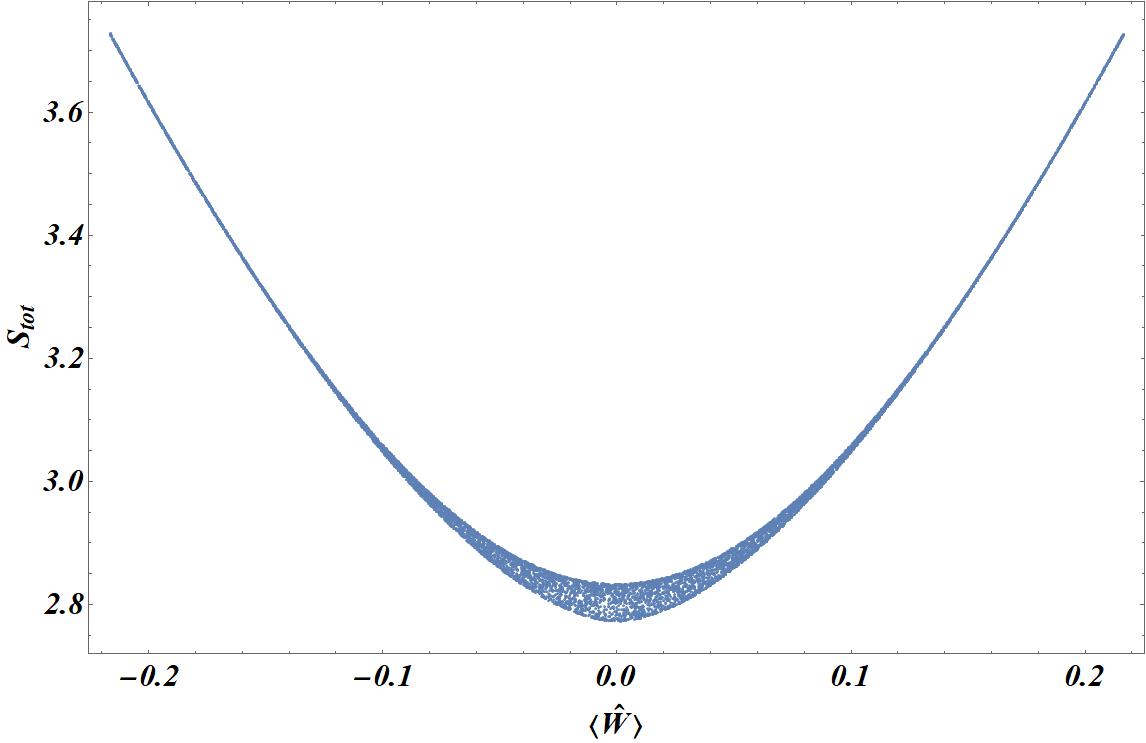
Figure 2: The relation between $S_{tot}=S_{12}+S_{13}+S_{14}$ and $\langle\hat{W}\rangle$.

Similarly, we consider this relation for $j=1$. The general state $\left|\psi_{4}\right\rangle$ reads as

$$\left|\psi_{4}\right\rangle = \alpha_{+}\left|\lambda_{+}\right\rangle+\alpha_{0}\left|\lambda_{0}\right\rangle+\alpha_{-}\left|\lambda_{-}\right\rangle,$$ (19)

where $\alpha_{\pm},\alpha_{0}$ are complex numbers. Then we have

$$\langle\hat{W}\rangle = \frac{\langle\psi_{4}|\hat{W}|\psi_{4}\rangle}{\langle\psi_{4}|\psi_{4}\rangle}=\frac{\sqrt{3}}{2}\frac{\left|\alpha_{+}\right|^{2}-\left|\alpha_{-}\right|^{2}}{\left|\alpha_{+}\right|^{2}+\left|\alpha_{0}\right|^{2}+\left|\alpha_{-}\right|^{2}},$$

$$\langle\hat{V}\rangle = \frac{\langle\psi_{4}|\hat{V}|\psi_{4}\rangle}{\left\langle\psi_{4}|\psi_{4}\right\rangle}=\left(\frac{\sqrt{3}}{2}\right)^{\frac{1}{2}}\frac{\left|\alpha_{+}\right|^{2}+\left|\alpha_{-}\right|^{2}}{\left|\alpha_{+}\right|^{2}+\left|\alpha_{0}\right|^{2}+\left|\alpha_{-}\right|^{2}}.$$ (20)

In Fig.3, we show the relation between $S_{tot}$ and $\langle\hat{W}\rangle$, $\langle\hat{V}\rangle$ with random numbers in intertwiner space. Again, our statement that $S_{tot}$ takes the maximal value for the eigenstates of $\langle\hat{W}\rangle$ is justified. In this case the relation between $S_{tot}$ and $\langle\hat{V}\rangle$ becomes complicated. But it is true that the maximal value of $S_{tot}$ appears when the expectation value of the volume takes the largest value. In addition, when the expectation value of the volume is zero, $S_{tot}$ takes the minimum. In Fig.3, all the corresponding $SU(2)$-invariant tensors are not prefect, even for the states with zero volume. This result further indicates that the quantum information has to lose its fidelity when teleporting through a four-valent $SU(2)$-invariant tensor.

In the end of this section we point out that the minimal deficit of the entanglement entropy $\Delta S\simeq 0.43$ for $j=1/2$, with the eigenvalue of $\langle\hat{V}\rangle=(\sqrt{3}/8)^{\frac{1}{2}}$, is smaller than $\Delta S\simeq 0.49$ for $j=1$, with the eigenvalue of $\langle\hat{V}\rangle=2(\sqrt{3}/8)^{\frac{1}{2}}$. This indicates that to build a quantum space with larger volume, the minimal deficit of entanglement entropy has to become larger as well. Intuitively, it implies that more information has to be stored in the space to form a space with larger volume. This observation could extend our previous conjecture to a more quantitative version: The space with non-zero volume must be built with non-perfect tensors. Furthermore, the larger the volume is, the more deficit of entanglement entropy for non-perfect tensors one has to pay.

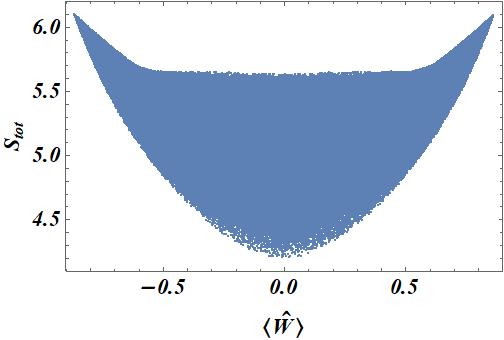
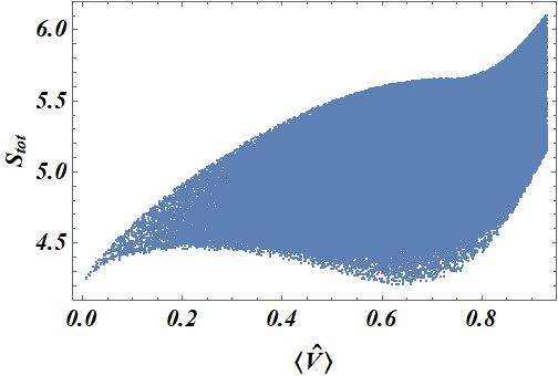
Figure 3: Left: The relation between $S_{tot}$ and $\langle\hat{W}\rangle$. Right: The relation between $S_{tot}$ and $\langle\hat{V}\rangle$.

V Conclusions and outlooks

In this note we have investigated the relations between the entanglement entropy of the boundary states and the geometric property of the quantum tetrahedron in the bulk for a single 4-valent vertex in the framework of spin networks. Qualitatively, we have conjectured that the emergence of the space with non-zero volume is the reflection of the non-perfectness of $SU(2)$-invariant tensors. Based on this conjecture, we might ascribe the increase or decrease of the space volume to the change of the entanglement among particles on the boundary. Inspired by this conjecture, it is quite interesting to explore the dynamics of space from the side of the evolution of entanglement at the Planck scale, for instance, at the beginning of the universe or the cosmological inflation scenario where the quantum effect of geometry becomes severe. Quantitatively, we have found the relation between the maximally entangled states and the eigenstates of the volume square operator. Interestingly enough, we have found that for $j=1/2$ and $j=1$, the boundary $SU(2)$-invariant states with the maximal entanglement entropy correspond to the eigenstates of the operator $\hat{W}$, which implies that the quantum tetrahedron has a definite orientation. It is intriguing to ask whether this correspondence also holds for other spins $j$. Our preliminary attempt indicates that for $j\geq 3/2$ there does not exist such simple relations between the states with the maximal entanglement entropy and the eigenstates of the operator $\hat{W}$. Their complicated relations deserve for further investigation.

Although $j=1/2$ and $j=1$ are just the specific cases for a four-valent states, this simple but elegant correspondence has significant implications for understanding the deep relations between the entanglement and the microscopic structure of the spacetime, particularly in a non-perturbative manner. As a microscopic scenario of quantum spacetime, representations of $j=1/2$ and $j=1$ are just like the ground state and the first excited state of the system, which should be dominantly occupied among all the possible distributions. This conjecture plays a key role in the original work on the microscopic interpretation on the entropy of black holes in terms of spin network statesAshtekar:1997yu .

The most desirable work next is to investigate the relations between quantum entanglement and quantum geometry in the framework of spin networks with more general setup. We expect to compute the entanglement entropy of a general boundary state, and explore its dependence on the orientation of the quantum polyhedrons in the bulk geometry. In this case, the main difficulty one faces is the involvement of holonomy along edges. Since the volume operator non-trivially acts only on intertwiner space at vertices, it is quite straightforward to discuss the geometric property of polyhedrons, but in general the entanglement of boundary states depends on the holonomy along edges, as previously studied in Ling:2018yaj . Our investigation on this topic is under progress.

Appendix

In this appendix we present the background on the spin network states with boundary, and then derive the $SU(2)$-invariant state with the maximal entanglement entropy for $j=1/2$. Given the connection $A$ and edge $e$, holonomy is defined as $h_{e}=Pexp\int_{e}A$. In irreducible representation of $SU(2)$, its matrix element is

$$R_{mn}^{j}(h_{e})=\left\langle j,n\right|h_{e}\left|j,m\right\rangle.$$ (21)

A closed spin network state can be represented by $\left|\Gamma,{j_{e}},{I_{v}}\right\rangle$, where $\Gamma$ is the graph composed of edges $e$, labelled by the representation $j_{e}$, and vertices $v$, labelled by the intertwiner $I_{v}$. The relationship between the spin network representation and the connection representation is given by

$$\left\langle h_{e_{1}},...,h_{e_{N}}|\Gamma,\{j_{e}\},\{I_{v}\}\right\rangle=\sum_{\{m_{e},n_{e}\}}\prod_{e\in E(\Gamma)}R_{m_{e}n_{e}}^{j_{e}}(h_{e})\prod_{v\in V(\Gamma)}(I_{v})_{\{m_{e},n_{e}\}}^{\{j_{e}\}}.$$ (22)

A spin network state with boundary can be represented by $\left|\Gamma,{j_{e},j_{l}},{I_{v}},{n_{l}}\right\rangle$, with $e$ for inner edges, $l$ for dangling edges where the magnetic quantum number $n_{l}$ is specified. The relationship between spin network representation and the connection representation is

$$\left\langle\{h_{e}\},\{h_{l}\}|\Gamma,\{j_{e},j_{l}\},\{I_{v}\},\{n_{l}\}\right\rangle = \sum_{m_{e},n_{e},m_{l}}\prod_{e\in E(\Gamma)}R_{m_{e}n_{e}}^{(j_{e})}(h_{e})$$ (23)

$$\times \prod_{v\in V(\Gamma)}(I_{v})_{\{m_{e}n_{e},m_{l}\}}^{\{j_{e},j_{l}\}}\prod_{l}R_{m_{l}n_{l}}^{j_{l}}(h_{l}).$$

Once $\Gamma$ and ${j_{e}}$ are specified, a spin network state with boundary can also be written as

$$\left|\Gamma,\{j_{e},j_{l}\},\{I_{v}\},\{n_{l}\}\right\rangle=\bigotimes_{v}\left|I_{v}^{\{j_{e},j_{l}\}}\right\rangle\bigotimes_{l}\left\langle j_{l},n_{l}\right|.$$ (24)

Thus $\left\langle\{h_{e}\},\{h_{l}\}\right|\bigotimes\left|{I_{v}}\right\rangle$ can be mapped to the right vector, $\left|\psi(\{h_{e}\},\{h_{l}\},\{I_{v}\})\right\rangle$, which is given as

$$\left|\psi(\{h_{e}\},\{h_{l}\},\{I_{v}\})\right\rangle = \sum_{n_{l}}\psi_{\{n_{l}\}}(\{h_{e}\},\{h_{l}\},\{I_{v}\})\prod_{l}\left|\{j_{l}\},\{n_{l}\}\right\rangle,$$ (25)

where

$$\psi_{n_{l}}(\{h_{e}\},\{h_{l}\},\{I_{v}\}) = \sum_{n_{l}^{\prime}}\psi_{\{n_{l}^{\prime}\}}(\{h_{e}\},\{h_{l}=I\},\{I_{v}\})R_{n_{l}^{\prime}n_{l}}^{j_{l}}(h_{l}),$$ (26)

$$\psi_{n_{l}}(\{h_{e}\},\{h_{l}=I\},\{I_{v}\}) = \sum_{m_{e},n_{e},m_{l},n_{l}}\prod_{e\in E(\Gamma)}R_{m_{e}n_{e}}^{j_{e}}(h_{e})\prod_{v\in V(\Gamma)}(I_{v})_{\{m_{e},n_{e},m_{l}\}}^{\{j_{e},j_{l}\}}\prod_{l}\delta_{m_{l}n_{l}},$$ (27)

with $I$ being the identity matrix. Usually, due to the presence of the boundary, the gauge invariance is broken. In this paper, we consider a simple network which only contains a single vertex associated with four dangling edges, so there is no $h_{e}$ and only one $I_{v}$ involved. The state is

$$\psi_{n_{1}n_{2}n_{3}n_{4}}(h_{1},h_{2},h_{3},h_{4},I_{v})$$

$$=\sum_{n_{1}^{\prime}n_{2}^{\prime}n_{3}^{\prime}n_{4}^{\prime}}\psi_{n_{1}^{\prime}n_{2}^{\prime}n_{3}^{\prime}n_{4}^{\prime}}(I,I,I,I,I_{v})R_{n_{1}^{\prime}n_{1}}^{j_{1}}(h_{1})R_{n_{2}^{\prime}n_{2}}^{j_{2}}(h_{2})R_{n_{3}^{\prime}n_{3}}^{j_{3}}(h_{3})R_{n_{4}^{\prime}n_{4}}^{j_{4}}(h_{4})$$

$$=\sum_{n_{1}^{\prime}n_{2}^{\prime}n_{3}^{\prime}n_{4}^{\prime}}(I_{v})_{n_{1}^{\prime}n_{2}^{\prime}n_{3}^{\prime}n_{4}^{\prime}}^{j_{1}j_{2}j_{3}j_{4}}R_{n_{1}^{\prime}n_{1}}^{j_{1}}(h_{1})R_{n_{2}^{\prime}n_{2}}^{j_{2}}(h_{2})R_{n_{3}^{\prime}n_{3}}^{j_{3}}(h_{3})R_{n_{4}^{\prime}n_{4}}^{j_{4}}(h_{4}),$$ (28)

where $j_{i}=j_{l_{i}},n_{i}=n_{l_{i}}(i=1,...,4)$ and $\psi_{n_{1}^{\prime}n_{2}^{\prime}n_{3}^{\prime}n_{4}^{\prime}}(I,I,I,I,I_{v})$ is a singlet and $SU(2)$ invariant.

Now we consider the entanglement entropy for such a 4-valent state with spin $j$. Without loss of generality, we consider the reduced density matrix by tracing the first and second index, leading to

$$(\rho_{34})_{n_{3}n_{4}n_{3}^{\prime}n_{4}^{\prime}}(h_{1},h_{2},h_{3},h_{4},I_{v})$$

$$=\sum_{n_{1}n_{2}}\sum_{n_{1}^{\prime\prime}n_{2}^{\prime\prime}n_{3}^{\prime\prime}n_{4}^{\prime\prime}}\psi_{n_{1}^{\prime\prime}n_{2}^{\prime\prime}n_{3}^{\prime\prime}n_{4}^{\prime\prime}}(I,I,I,I,I_{v})R_{n_{1}^{\prime\prime}n_{1}}^{j_{1}}(h_{1})R_{n_{2}^{\prime\prime}n_{2}}^{j_{2}}(h_{2})R_{n_{3}^{\prime\prime}n_{3}}^{j_{3}}(h_{3})R_{n_{4}^{\prime\prime}n_{4}}^{j_{4}}(h_{4})$$

$$\times\sum_{n_{1}^{\prime\prime\prime}n_{2}^{\prime\prime\prime}n_{3}^{\prime\prime\prime}n_{4}^{\prime\prime\prime}}\psi_{n_{1}^{\prime\prime\prime}n_{2}^{\prime\prime\prime}n_{3}^{\prime\prime\prime}n_{4}^{\prime\prime\prime}}^{*}(I,I,I,I,I_{v})R_{n_{1}^{\prime\prime\prime}n_{1}}^{j_{1}*}(h_{1})R_{n_{2}^{\prime\prime\prime}n_{2}}^{j_{2}*}(h_{2})R_{n_{3}^{\prime\prime\prime}n_{3}^{\prime}}^{j_{3}*}(h_{3})R_{n_{4}^{\prime\prime\prime}n_{4}^{\prime}}^{j_{4}*}(h_{4}).$$ (29)

We remark that for a single vertex, the entanglement entropy does not depend on $(h_{1},h_{2},h_{3},h_{4})$ because all the reduced density matrices are related by similarity transformations. Thus one can simply set them be identity matrix $I$, leading to the reduced density matrix for a $SU(2)$-invariant tensor. Applying Eq.(2), one has

$$(\rho_{34})_{n_{3}n_{4}n_{3}^{\prime}n_{4}^{\prime}}(I_{v})\propto\sum_{J=0}^{2j}\frac{|\alpha(J)|^{2}}{2J+1}\sum_{M}C_{n_{3}n_{4}JM_{1}}^{(jj)}C_{n_{3}^{\prime}n_{4}^{\prime}JM_{1}}^{(jj)}.$$ (30)

Due to the unitarity of $CG$ coefficients, one can show that

$$\rho_{34}\sim\frac{1}{\sum_{J=0}^{2j}|\alpha(J)|^{2}}diag\left[(|\alpha(0)|^{2})^{\oplus 1},(\frac{1}{3}|\alpha(1)|^{2})^{\oplus 3},...,(\frac{1}{2j+1}|\alpha(j)|^{2})^{\oplus(2j+1)}\right].$$ (31)

Then we derive the entanglement entropy as

$$S_{34}=(\sum_{J=0}^{2j}|\alpha(J)|^{2})^{-1}(-\sum_{J=0}^{2j}|\alpha(J)|^{2}\ln\frac{|\alpha(J)|^{2}}{2J+1})+\ln\sum_{J=0}^{2j}|\alpha(J)|^{2}.$$ (32)

Similarly, $\left|\psi_{4}\right\rangle$ can also be expanded based on other basis in intertwiner space as

$$\psi_{m_{1}m_{2}m_{3}m_{4}}=\sum_{J}\frac{\beta(J)}{\sqrt{2J+1}}\sum_{M_{1}M_{2}}C_{m_{1}m_{3}JM_{1}}^{(j_{1}j_{3})}C_{m_{4}m_{2}JM_{2}}^{(j_{4}j_{2})}D^{(J)M_{1}M_{2}},$$ (33)

$$\psi_{m_{1}m_{2}m_{3}m_{4}}=\sum_{J}\frac{\gamma(J)}{\sqrt{2J+1}}\sum_{M_{1}M_{2}}C_{m_{1}m_{4}JM_{1}}^{(j_{1}j_{4})}C_{m_{2}m_{3}JM_{2}}^{(j_{2}j_{3})}D^{(J)M_{1}M_{2}},$$ (34)

which is very convenient for us to calculate the entanglement entropy for other bipartitions. Specifically, we have

$$S_{24}=(\sum_{J=0}^{2j}|\beta(J)|^{2})^{-1}(-\sum_{J=0}^{2j}|\beta(J)|^{2}\ln\frac{|\beta(J)|^{2}}{2J+1})+\ln\sum_{J=0}^{2j}|\beta(J)|^{2},$$

$$S_{23}=(\sum_{J=0}^{2j}|\gamma(J)|^{2})^{-1}(-\sum_{J=0}^{2j}|\gamma(J)|^{2}\ln\frac{|\gamma(J)|^{2}}{2J+1})+\ln\sum_{J=0}^{2j}|\gamma(J)|^{2}.$$ (35)

Next we will determine the values of parameters $\alpha(J),\beta(J),\gamma(J)$ such that the sum of the entanglement entropy will take the maximal value among all the possible states. First of all, since $\alpha(J),\beta(J),\gamma(J)$ are parameters in different representations of the same state, they must be related to one another, we intend to derive their relations at first. One can easily find that $\left\langle\psi_{4}|\psi_{4}\right\rangle=\sum_{J=0}^{2j}|\alpha(J)|^{2}=\sum_{J=0}^{2j}|\beta(J)|^{2}=\sum_{J=0}^{2j}|\gamma(J)|^{2}=:U$, obviously $U>0$. Therefore, the sum of entanglement entropy reads as

$$S_{tot}=U^{-1}(-\sum_{J=0}^{2j}|\alpha(J)|^{2}\ln\frac{|\alpha(J)|^{2}}{2J+1}-\sum_{J=0}^{2j}|\beta(J)|^{2}\ln\frac{|\beta(J)|^{2}}{2J+1}-\sum_{J=0}^{2j}|\gamma(J)|^{2}\ln\frac{|\gamma(J)|^{2}}{2J+1})+3\ln U.$$ (36)

From Eq. (2) and Eq. (33), one has

$$\sum_{J^{\prime}}\frac{\alpha(J^{\prime})}{\sqrt{2J^{\prime}+1}}\sum_{M_{1}^{\prime}M_{2}^{\prime}}C_{m_{1}m_{2}J^{\prime}M_{1}^{\prime}}^{(j_{1}j_{2})}C_{m_{3}m_{4}J^{\prime}M_{2}^{\prime}}^{(j_{3}j_{4})}D^{(J^{\prime})M_{1}^{\prime}M_{2}^{\prime}}$$ (37)

$$= \sum_{J}\frac{\beta(J))}{\sqrt{2J+1}}\sum_{M_{1}M_{2}}C_{m_{1}m_{3}JM_{1}}^{(j_{1}j_{3})}C_{m_{4}m_{2}JM_{2}}^{(j_{4}j_{2})}D^{(J)M_{1}M_{2}}.$$

From this equality, one can derive the following equation

$$\sum_{m_{1}m_{2}m_{3}m_{4}}\sum_{J^{\prime}}\frac{\alpha(J^{\prime})}{2J+1}\sum_{M_{1^{\prime}}M_{2^{\prime}}}C_{m_{1}m_{2}J^{\prime}M_{1}^{\prime}}^{(j_{1}j_{2})}C_{m_{3}m_{4}J^{\prime}M_{2}^{\prime}}^{(j_{3}j_{4})}D^{(J^{\prime})M_{1}^{\prime}M_{2}^{\prime}}C_{m_{1}m_{3}J^{\prime\prime}M_{1}^{\prime\prime}}^{(j_{1}j_{3})*}C_{m_{4}m_{2}J^{\prime\prime}M_{2}^{\prime\prime}}^{(j_{4}j_{2})*}$$ (38)

$$= \sum_{m_{1}m_{2}m_{3}m_{4}}\sum_{J}\frac{\beta(J)}{2J+1}\sum_{M_{1}M_{2}}C_{m_{1}m_{3}JM_{1}}^{(j_{1}j_{3})}C_{m_{4}m_{2}JM_{2}}^{(j_{4}j_{2})}D^{(J)M_{1}M_{2}}C_{m_{1}m_{3}J^{\prime\prime}M_{1}^{\prime\prime}}^{(j_{1}j_{3})*}C_{m_{4}m_{2}J^{\prime\prime}M_{2}^{\prime\prime}}^{(j_{4}j_{2})*}$$

$$= \sum_{J}\frac{\beta(J)}{2J+1}\sum_{M_{1},M_{2}}\delta_{J}^{J^{\prime\prime}}\delta_{M_{1}}^{M_{1}^{\prime\prime}}\delta_{J}^{J^{\prime\prime}}\delta_{M_{2}}^{M_{2}^{\prime\prime}}D^{(J)M_{1}M_{2}}$$

$$= \frac{\beta(J^{\prime\prime})}{2J^{\prime\prime}+1}D^{(J^{\prime\prime})M_{1}^{\prime\prime}M_{2}^{\prime\prime}}.$$

Therefore, the term, $C_{m_{1}m_{2}JM_{1}^{\prime}}^{(j_{1}j_{2})}C_{m_{3}m_{4}JM_{2}^{\prime}}^{(j_{3}j_{4})}D^{(J^{\prime})M_{1}^{\prime}M_{2}^{\prime}}C_{m_{1}m_{3}J^{\prime\prime}M_{1}}^{(j_{1}j_{3})*}C_{m_{4}m_{2}J^{\prime\prime}M_{2}}^{(j_{4}j_{2})*}$, has $SU(2)$-invariance for $M_{1},M_{2}$. So let

$$C_{m_{1}m_{2}J^{\prime}M_{1}^{\prime}}^{(j_{1}j_{2})}C_{m_{3}m_{4}J^{\prime}M_{2}^{\prime}}^{(j_{3}j_{4})}D^{(J^{\prime})M_{1}^{\prime}M_{2}^{\prime}}C_{m_{1}m_{3}JM_{1}}^{(j_{1}j_{3})*}C_{m_{4}m_{2}JM_{2}}^{(j_{4}j_{2})*}=N(j,J^{\prime},J)D^{(J)M_{1}M_{2}}.$$ (39)

Then, we find the intertwiner parameters in different representations are related by

$$\beta(J)=\sqrt{2J+1}\sum_{J^{\prime}}N(j,J^{\prime},J)\frac{\alpha(J)}{\sqrt{2J^{\prime}+1}}.$$ (40)

For the same reason, one has

$$\gamma(J)=\sqrt{2J+1}\sum_{J^{\prime}}N^{\prime}(j,J^{\prime},J)\frac{\alpha(J)}{\sqrt{2J^{\prime}+1}},$$ (41)

where $N^{\prime}(j,J^{\prime},J)$ satisfies

$$C_{m_{1}m_{2}J^{\prime}M_{1}^{\prime}}^{(j_{1}j_{2})}C_{m_{3}m_{4}JM_{2}^{\prime}}^{(j_{3}j_{4})}D^{(J^{\prime})M_{1}^{\prime}M_{2}^{\prime}}C_{m_{1}m_{4}JM_{1}}^{(j_{1}j_{4})*}C_{m_{2}m_{3}JM_{2}}^{(j_{2}j_{3})*}=N^{\prime}(j,J^{\prime},J)D^{(J)M_{1}M_{2}}.$$ (42)

We point out that $N(j,J^{\prime},J),N^{\prime}(j,J^{\prime},J)$ can be explicitly calculated by $6j$ symbols.

$$N(j,J^{\prime},J)=(2J^{\prime}+1)(-1)^{J^{\prime}}\begin{pmatrix}j&j&J\\ j&j&J^{\prime}\end{pmatrix},$$

$$N^{\prime}(j,J^{\prime},J)=(2J^{\prime}+1)(-1)^{J}\begin{pmatrix}j&j&J\\ j&j&J^{\prime}\end{pmatrix}.$$ (43)

Above equations give the general relations for parameters $\alpha(J),\beta(J),\gamma(J)$. Now we focus on the simple cases with specific spin $j$. When $j=1/2$, then $J=0,\ 1$. The non-trivial $6j$ symbols are

$$\begin{pmatrix}\frac{1}{2}&\frac{1}{2}&0\\ \frac{1}{2}&\frac{1}{2}&0\end{pmatrix}=-\frac{1}{2},\ \begin{pmatrix}\frac{1}{2}&\frac{1}{2}&0\\ \frac{1}{2}&\frac{1}{2}&1\end{pmatrix}=\frac{1}{2},\ \begin{pmatrix}\frac{1}{2}&\frac{1}{2}&1\\ \frac{1}{2}&\frac{1}{2}&0\end{pmatrix}=\frac{1}{2},\ \begin{pmatrix}\frac{1}{2}&\frac{1}{2}&1\\ \frac{1}{2}&\frac{1}{2}&1\end{pmatrix}=-\frac{1}{6},\$$ (44)

which give rise to the following relations for $\alpha(J),\beta(J),\gamma(J)$

$$\beta(0)=-\frac{1}{2}\alpha(0)-\frac{\sqrt{3}}{2}\alpha(1),\ \beta(1)=\frac{\sqrt{3}}{2}\alpha(0)-\frac{1}{2}\alpha(1),$$

$$\gamma(0)=-\frac{1}{2}\alpha(0)+\frac{\sqrt{3}}{2}\alpha(1),\ \gamma(1)=-\frac{\sqrt{3}}{2}\alpha(0)-\frac{1}{2}\alpha(1).$$ (45)

As a result, we find the sum of the entanglement entropy is

$$S_{tot} = U^{-1}(-|\alpha(0)|^{2}\ln|\alpha(0)|^{2}-|\beta(0)|^{2}\ln|\beta(0)|^{2}-|\gamma(0)|^{2}\ln|\gamma(0)|^{2}$$ (46)

$$- |\alpha(1)|^{2}\ln|\alpha(1)|^{2}/3-|\beta(1)|^{2}\ln|\beta(1)|^{2}/3-|\gamma(1)|^{2}\ln|\gamma(1)|^{2}/3)+3\ln U.$$

Furthermore, from Eq.(45), one can derive that

$$|\alpha(1)|^{2}+|\beta(1)|^{2}+|\gamma(1)|^{2}=|\alpha(0)|^{2}+|\beta(0)|^{2}+|\gamma(0)|^{2}=\frac{3}{2}(|\alpha(0)|^{2}+|\alpha(1)|^{2})=\frac{3}{2}U.$$ (47)

By virtue of the inequality $\ln x\leq x-1(x>0)$, one can show that

$$-|\alpha(0)|^{2}\ln(|\alpha(0)|^{2}) \leq \frac{U}{2}-\ln(\frac{U}{2})|\alpha(0)|^{2},$$

$$|\alpha(1)|^{2}\ln|\alpha(1)|^{2}/3 \leq U/2-|\alpha(1)|^{2}-\ln(U/6)|\alpha(1)|^{2}.$$ (48)

Similar inequality can be derived for $\beta$ and $\gamma$. Where the equal sign of the inequality holds if and only if $|\alpha(0)|^{2}=|\beta(0)|^{2}=|\gamma(0)|^{2}=|\alpha(1)|^{2}=|\beta(1)|^{2}=|\gamma(1)|^{2}=U/2$, which leads to

$$\alpha(1)/\alpha(0)=\pm i,\ \ with\ \ \alpha(0)\neq 0.$$ (49)

So ignoring the phase factor, there are two maximally entangled states. They are

$$\frac{1}{\sqrt{2}}\left|J=0\right\rangle\pm\frac{i}{\sqrt{2}}\left|J=1\right\rangle.$$ (50)

Similarly, one can determine the intertwiner parameters for $j=1$ and analytically derive $SU(2)$-invariant states with the maximal entanglement entropy.

References

- (1) J. M. Maldacena, JHEP 0304, 021 (2003) [hep-th/0106112].
- (2) S. Ryu and T. Takayanagi, Phys. Rev. Lett. 96, 181602 (2006) [hep-th/0603001].
- (3) M. Van Raamsdonk, Gen. Rel. Grav. 42, 2323 (2010) [Int. J. Mod. Phys. D 19, 2429 (2010)] [arXiv:1005.3035 [hep-th]].
- (4) G. Vidal, Phys. Rev. Lett. 99, no. 22, 220405 (2007) [cond-mat/0512165].
- (5) B. Swingle, Phys. Rev. D 86, 065007 (2012) [arXiv:0905.1317 [cond-mat.str-el]].
- (6) B. Swingle, arXiv:1209.3304 [hep-th].
- (7) D. Harlow, Commun. Math. Phys. 354, no. 3, 865 (2017) [arXiv:1607.03901 [hep-th]].
- (8) F. Pastawski, B. Yoshida, D. Harlow and J. Preskill, JHEP 1506, 149 (2015) [arXiv:1503.06237 [hep-th]].
- (9) Y. Ling, Y. Liu, Z. Y. Xian and Y. Xiao, Phys. Rev. D 99, no. 2, 026008 (2019) [arXiv:1806.05007 [hep-th]].
- (10) Y. Ling, Y. Liu, Z. Y. Xian and Y. Xiao, JHEP 1906, 032 (2019) [arXiv:1807.10247 [hep-th]].
- (11) R. Orus, Eur. Phys. J. B 87, 280 (2014) [arXiv:1407.6552 [cond-mat.str-el]].
- (12) M. Han and L. Y. Hung, Phys. Rev. D 95, no. 2, 024011 (2017) [arXiv:1610.02134 [hep-th]].
- (13) Y. Li, M. Han, M. Grassl and B. Zeng, New J. Phys. 19, no. 6, 063029 (2017) [arXiv:1612.04504 [quant-ph]].
- (14) Y. Li, M. Han, D. Ruan and B. Zeng, J. Phys. A 51, no. 17, 175303 (2018) [arXiv:1709.08370 [quant-ph]].
- (15) G. Chirco, D. Oriti and M. Zhang, Class. Quant. Grav. 35, no. 11, 115011 (2018) [arXiv:1701.01383 [gr-qc]].
- (16) G. Chirco, F. M. Mele, D. Oriti and P. Vitale, Phys. Rev. D 97, no. 4, 046015 (2018) [arXiv:1703.05231 [gr-qc]].
- (17) E. R. Livine, Phys. Rev. D 97, no. 2, 026009 (2018) [arXiv:1709.08511 [gr-qc]].
- (18) B. Baytas, E. Bianchi and N. Yokomizo, Phys. Rev. D 98, no. 2, 026001 (2018) [arXiv:1805.05856 [gr-qc]].
- (19) Y. Ling, M. H. Wu and Y. Xiao, Chin. Phys. C 43, no. 1, 013106 (2019) [arXiv:1811.03213 [hep-th]].
- (20) C. Rovelli and L. Smolin, Nucl. Phys. B 442, 593 (1995) Erratum: [Nucl. Phys. B 456, 753 (1995)] [gr-qc/9411005].
- (21) C. Rovelli and L. Smolin, Phys. Rev. D 52, 5743 (1995) [gr-qc/9505006].
- (22) R. Loll, Phys. Rev. Lett. 75, 3048 (1995) [gr-qc/9506014].
- (23) R. De Pietri and C. Rovelli, Phys. Rev. D 54, 2664 (1996) [gr-qc/9602023].
- (24) A. Ashtekar and J. Lewandowski, Adv. Theor. Math. Phys. 1, 388 (1998) [gr-qc/9711031].
- (25) T. Thiemann, J. Math. Phys. 39, 3347 (1998) [gr-qc/9606091].
- (26) K. Giesel and T. Thiemann, Class. Quant. Grav. 23, 5667 (2006) [gr-qc/0507036].
- (27) K. Giesel and T. Thiemann, Class. Quant. Grav. 23, 5693 (2006) [gr-qc/0507037].
- (28) J. Yang and Y. Ma, Eur. Phys. J. C 77, no. 4, 235 (2017) [arXiv:1505.00223 [gr-qc]].
- (29) A. Ashtekar, J. Baez, A. Corichi and K. Krasnov, Phys. Rev. Lett. 80, 904 (1998) [gr-qc/9710007].