Finding Outliers in Gaussian Model-Based Clustering

Abstract

Unsupervised classification, or clustering, is a problem often plagued by outliers, yet there is a paucity of work on handling outliers in unsupervised classification. Outlier algorithms tend to fall into two broad categories: outlier inclusion methods and trimming methods, which often require pre-specification of the number of points to remove. The fact that sample Mahalanobis distance is beta-distributed is used to derive an approximate distribution for the log-likelihoods of subset finite Gaussian mixture models. An algorithm is proposed that removes the least likely points, which are deemed outliers, until the log-likelihoods adhere to the reference distribution. This results in a trimming method which inherently estimates the number of outliers present.

Keywords: Clustering; model selection; mixture models; outlier.

Classification aims to partition data into a set number of groups, whereby observations in the same group are in some sense similar to one another. Clustering is unsupervised classification, in that none of the group memberships are known a priori. Most clustering algorithms originate from one of three major methods: hierarchical clustering, partition-based methods such as $k$-means clustering, and mixture model-based clustering. Although hierarchical and partition-based clustering remain popular, the mixture modelling approach has become increasingly prevalent due to its robustness and mathematical interpretability (McNicholas, 2016). In the mixture modelling framework for clustering, each component is usually taken to be a cluster. Although the model can employ almost any component distribution, Gaussian components remain popular due to the distribution’s versatility and ubiquity. Most mixture model-based clustering methods assume, either explicitly or implicitly, that the data are free of outliers.

Mixture model-based clustering involves maximizing the likelihood of the mixture model. The density of a Gaussian mixture model is a convex linear combination of each component density and is given by

$$f(\mathbf{x}\mid\boldsymbol{\vartheta})=\sum_{g=1}^{G}\pi_{g}\phi(\mathbf{x}\mid\boldsymbol{\mu}_{g},\mathbf{\Sigma}_{g}),$$ (1)

where

$$\phi(\mathbf{x}\mid\boldsymbol{\mu}_{g},\mathbf{\Sigma}_{g})=\frac{1}{\sqrt{(2\pi)^{p}|\mathbf{\Sigma}_{g}|}}\text{exp}\left\{-\frac{1}{2}(\mathbf{x}-\boldsymbol{\mu}_{g})^{\prime}\mathbf{\Sigma}_{g}^{-1}(\mathbf{x}-\boldsymbol{\mu}_{g})\right\}$$

is the density of a $p$-dimensional random variable $\mathbf{X}$ from a Gaussian distribution with mean $\boldsymbol{\mu}_{g}$ and covariance matrix $\mathbf{\Sigma}_{g}$, $\pi_{g}>0$ is the mixing proportion such that $\sum_{g=1}^{G}\pi_{g}=1$, and $\boldsymbol{\vartheta}=\{\pi_{1},\dots,\pi_{G},\boldsymbol{\mu}_{1},\dots,\boldsymbol{\mu}_{G},\mathbf{\Sigma}_{1},\dots,\mathbf{\Sigma}_{G}\}$.

An outlier can be considered an observation “that appears to deviate markedly from other members of the sample in which it occurs” (Grubbs, 1969). The two main types of outliers are gross outliers, which do not exist in close proximity to the desired data, and technical outliers, which may be near but are unusual relative to the structure of the data. Outliers may occur due to (unlikely) random chance, or they may arise due to experimental, measurement, or recording error.

Consider a simulated noisy dataset, such as the one in Figure 1. We simulate three Gaussian clusters with uniform noise (outliers) and use the mixture (Pocuca et al., 2021) package in R (R Core Team, 2021) to cluster the data into three groups. By failing to account for outliers, traditional clustering using a Gaussian mixture model results in a two-cluster solution with some outliers forming their own cluster. This results in an ill-fitting model which misclassifies the data and also misrepresents the number of clusters. In addition, outliers, particularly those with high leverage, can significantly affect the parameter estimates. When fitting a model, they may draw the sample mean towards them and inflate the sample variance. In the case of our simulated example, the originally spherical clusters are elongated and rotated. It is thus beneficial to remove, or reduce, the effect of outliers by accounting for them in the model.

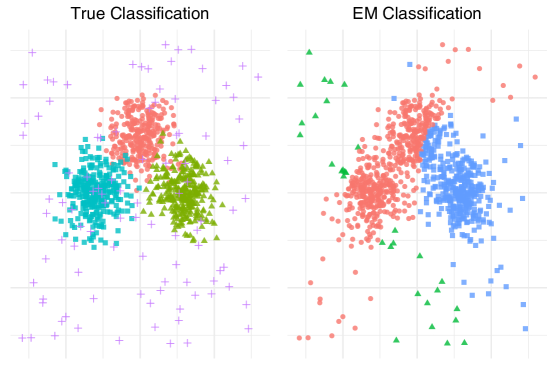
Figure 1: A simulated example of a noisy dataset.

1 Related Work

1.1 Outliers in Unsupervised Model-Based Clustering

In model-based clustering, outlier algorithms usually fall into two paradigms– outlier-inclusion and outlier trimming. The first method, proposed by Banfield and Raftery (1993), includes outliers in an additional uniform component over the convex hull. If outliers are cluster-specific, we can incorporate them into the tails if we cluster using mixtures of t-distributions (Peel and McLachlan, 2000). Punzo and McNicholas (2016) introduce mixtures of contaminated Gaussian distributions, where each cluster has a proportion $\alpha_{g}\in(0,1)$ of ‘good’ points with density $\phi(\mathbf{x}\mid\boldsymbol{\mu}_{g},\mathbf{\Sigma}_{g})$, and a proportion $1-\alpha_{g}$ of ‘bad’ points, with density $\phi(\mathbf{x}\mid\boldsymbol{\mu}_{g},\eta_{g}\mathbf{\Sigma}_{g})$. Each distribution has the same centre, but the ‘bad’ points have an inflated variance, where $\eta_{g}>1$.

Instead of fitting outliers in the model, it may be of interest to trim them from the dataset. Cuesta-Albertos et al. (1997) developed an impartial trimming approach for $k$-means clustering; however, this method maintains the drawback of $k$-means clustering, where the clusters are spherical with equal — or, in practice, similar — radii or they are so well separated that a departure from this shape constraint will not matter. Of course, the latter is a trivial case and is mentioned only for completeness. García-Escudero et al. (2008) improved upon trimmed $k$-means with the TCLUST algorithm. TCLUST places a restriction on the eigenvalue ratio of the covariance matrix, as well as implementing a weight on the clusters, allowing for clusters of various elliptical shapes and sizes. An obvious challenge with these methods is that the eigenvalue ratio must also be known a priori. There exists an estimation scheme for the proportion of outliers, denoted $\alpha$, but it is heavily influenced by the choices for number of clusters and eigenvalue ratio. It is of great interest to bring trimming into the model-based clustering domain, especially when $\alpha$ is unknown. This is the case for most real datasets — in fact, for all but very low dimensional data.

1.2 General Unsupervised Outlier Detection Methods

Some traditional approaches to outlier analysis identify points with outlier scores greater than a certain threshold. Often, points are considered outliers if their scores are outside the interval $(a-bx,a+bx)$, where $a$ is a measure of central tendency, and $x$ is a measure of variability. Examples include the three sigma rule and the median absolute difference thresholding strategy (Hampel, 1974). Yang et al. (2019) make this method robust by applying the thresholding procedure twice, while Buzzi-Ferraris and Manenti (2011) remove outliers one-by-one by iteratively applying a clever mean threshold.

In the clustering framework, similar outlier scores can be generated using the distance to the cluster centre (Hautamäki et al., 2005) or to the $k$-nearest neighbours (Ramaswamy et al., 2000). We can also consider points of low density to be outliers, for example in Knorr and Ng (1998), where points with few neighbours within a specified distance are identified, or DBSCAN (Ester et al., 1996), which clusters data based on density, with points not placed in clusters classified as noise. Fränti and Yang (2018) smooth noisy data by replacing each point by the mean of its $k$-nearest neighbours. They repeat this process several times to obtain better centroid locations and $k$-means classification. Yang et al. (2021) take this one step further by treating the distance each point is shifted as an outlier score.

Boukerche et al. (2020) provide a detailed survey of methods to address outliers in unsupervised classification. They include approaches which are proximity- or projection-based, and techniques for high-dimensional, streaming, or ‘big’ data. While these methods could be used to identify observations that deviate from the entire dataset, some cannot consider points which are spurious in relation to the cluster structure. Although this paper includes cluster-based approaches, the mentioned methods mainly consider groups of outliers which form their own cluster.

Liu et al. (2019) propose an unsupervised multiple-objective generative adversarial active learning (MO-GAAL) method, which generates potential outliers to train a classifier. Iteratively, the generators are able learn the generation mechanism of the data, while the discriminators predict the probability that the sample comes from the real data. The result is a boundary which aims to separate the outliers from the normal datapoints.

1.3 Other Outlier Detection Methods

The foregoing has focused on unsupervised methods on the topic of outliers. Before proceeding, it is worth considering the field more broadly so that the work discussed herein is put in proper context. Domingues et al. (2018) present a recent review and comparison of “unsupervised machine learning algorithms in the context of outlier detection”. While several approaches are considered by Domingues et al. (2018), they operate within a scenario where a training set is used for tuning and the approach is then evaluated on a test, or hold-out, set. This is a fundamentally different paradigm from that considered herein, where we operate within a completely unsupervised paradigm. That is, for every observation, no a priori knowledge of whether an observation is an outlier or to what class it belongs is used to tune an algorithm or estimate model parameters.

Novelty detection is a related area of endeavour within the pattern recognition literature, where the scenario is that test data are encountered that seem in some respect anomalous when compared to the training data that were used for tuning. Again, the paradigm considered herein is different in that there is no training or test stage; rather, we consider unsupervised classification with outliers. However, the interested reader is referred to Pimentel et al. (2014) for a review of approaches to novelty detection.

2 Methodology

2.1 Distribution of Log-Likelihoods

In this section, we use the distribution of Mahalanobis squared distance to derive the distribution of subset log-likelihoods, which forms the basis for the proposed OCLUST algorithm. We consider a subset log-likelihood to be the log-likelihood of a model fitted with $n-1$ of the data points. Formally, if we denote our complete dataset as $\mathcal{X}=\{\mathbf{x}_{1},\dots,\mathbf{x}_{n}\}$, then we can define the $j$th subset as the complete dataset with the $j$th point removed, $\mathcal{X}\setminus\mathbf{x}_{j}=\{\mathbf{x}_{1},\dots,\mathbf{x}_{j-1},\mathbf{x}_{j+1},\dots,\mathbf{x}_{n}\}$. There are $n$ of these such subsets.

Consider a dataset $\mathcal{X}=\{\mathbf{x}_{1},\dots,\mathbf{x}_{n}\}$ in $p$-dimensional Euclidian space $\mathbb{R}^{p}$, where each $\mathbf{x}_{i}\in\mathcal{X}$ has Gaussian mixture model density $f(\mathbf{x}_{i}\mid\boldsymbol{\vartheta})$ as in (1). The log-likelihood of dataset $\mathcal{X}$ under the Gaussian mixture model is

$$\ell_{\mathcal{X}}=\sum_{i=1}^{n}\log\left[\sum_{g=1}^{G}\pi_{g}\phi(\mathbf{x}_{i}\mid\boldsymbol{\mu}_{g},\mathbf{\Sigma}_{g})\right].$$ (2)

The log-likelihood of a model with $n-1$ points is usually larger than the log-likelihood with $n$ points because the joint density is multiplied by one fewer point, and a multivariate Gaussian density tends to be less than one. Points with low density near the tails will increase the log-likelihood by a greater extent than points with higher density, near the centre of the distribution. Intuitively, the more the log-likelihood increases, the more outlying the point was; the model improved the most in its absence.

By this logic, we treat point $\mathbf{x}_{k}$, whose absence produced the largest subset log-likelihood, as our candidate outlier. Formally, we can express this as follow,

Definition 1 (Candidate Outlier).

We define our candidate outlier as $\mathbf{x}_{k}$, where

$$k=\arg\max_{j\in[1,n]}\ell_{\mathcal{X}\setminus\mathbf{x}_{j}},$$

and $\ell_{\mathcal{X}\setminus\mathbf{x}_{j}}$ is the log-likelihood of the subset model with the jth point removed.

We continue removing candidate outliers until we obtain our best model, which is determined by the distribution of our subset log-likelihoods, derived below. Note that a beta random variable $W$ has density

$$f_{\text{beta}}(w|\alpha,\beta)=\frac{\Gamma(\alpha+\beta)}{\Gamma(\alpha)\Gamma(\beta)}w^{\alpha-1}(1-w)^{\beta-1}.$$ (3)

Proposition 1.

For a point $\mathbf{x}_{j}$ belonging to the $h$th cluster, if $Q_{\mathcal{X}}$ is a simplified log-likelihood and $Y_{j}=Q_{\mathcal{X}\setminus\mathbf{x}_{j}}-Q_{\mathcal{X}}$, then $Y_{j}$ has an approximate shifted and scaled beta density

$$Y_{j}\sim f_{\text{beta}}\left(\frac{2n_{h}}{(n_{h}-1)^{2}}(y_{j}-c)~{}\bigg{|}~{}\frac{p}{2},\frac{n_{h}-p-1}{2}\right),$$ (4)

for $y_{j}-c\geq 0,\alpha>0,\beta>0$, and where $c=-\log\pi_{h}+\frac{p}{2}\log(2\pi)+\frac{1}{2}\log\lvert\mathbf{S}_{h}\rvert$, $n_{h}$ is the number of points in cluster $h$, $\mathbf{S}_{h}$ is the sample variance of cluster $h$, and $\pi_{h}=n_{h}/n$.

The mathematical results for this proposition are shown in the following lemmata. However, we must first simplify our log-likelihood. In (2), each cluster contributes to the density of every point. Instead, consider the case where the clusters are well-separated. We can develop a simplified log-likelihood, which we will call $Q_{\mathcal{X}}$, which only considers the density of the component to which the point belongs. We formalize this result in Assumption 1 and Lemma 1.

Assumption 1.

The clusters are non-overlapping and well separated.

Assumption 1 is required for Lemma 1. In practice, however, these assumptions may be relaxed. For more information on the effect of cluster separation on the density, see  Appendix A.

Write $\mathbf{x}_{i}\in\mathcal{C}_{g}$ to indicate that $\mathbf{x}_{i}$ belongs to the $g$th cluster. Let $\mathbf{z}_{i}=(z_{i1},\ldots,z_{iG})^{\prime}$, where $z_{ig}=1$ if $\mathbf{x}_{i}\in\mathcal{C}_{g}$ and $z_{ig}=0$ if $\mathbf{x}_{i}\notin\mathcal{C}_{g}$.

Lemma 1.

As the separation between the clusters increases, $\ell_{\mathcal{X}}\simeq Q_{\mathcal{X}}$. In other words, the log-likelihood in (2) converges asymptotically to $Q_{\mathcal{X}}$, where

$$Q_{\mathcal{X}}=\sum_{i=1}^{n}\sum_{g=1}^{G}z_{ig}\left[\log\pi_{g}+\log\phi(\mathbf{x}_{i}\mid\boldsymbol{\mu}_{g}.\mathbf{\Sigma}_{g})\right]=\sum_{\mathbf{x}_{i}\in\mathcal{C}_{g}}\left[\log\pi_{g}+\log\phi(\mathbf{x}_{i}\mid\boldsymbol{\mu}_{g}.\mathbf{\Sigma}_{g})\right].$$

A proof of Lemma 1 may be found in Appendix B. We will maintain Assumption 1 throughout this paper. $Q_{\mathcal{X}}$ can be regarded as the simplified log-likelihood for the entire dataset $\mathcal{X}$. We define $Q_{\mathcal{X}\setminus\mathbf{x}_{j}}$ as the simplified log-likelihood for the $j$th subset $\mathcal{X}\setminus\mathbf{x}_{j}$. Finally, we define the variable $Y_{j}=Q_{\mathcal{X}\setminus\mathbf{x}_{j}}-Q_{\mathcal{X}}$ as the difference between the $j$th subset log-likelihood and the log-likelihood for the whole dataset.

Assumption 2.

The number of observations in each cluster, $n_{g}$, is large.

This assumption is required to make use of the asymptotic properties of the parameter estimates. We must estimate our parameters because these are unknown in unsupervised classification. Due to their desirable qualities, we will replace $\boldsymbol{\mu}_{g}$ and $\mathbf{\Sigma}_{g}$ by their unbiased estimates:

$$\begin{split}\hat{\boldsymbol{\mu}}_{g}&=\bar{\mathbf{x}}_{g}=\frac{1}{n_{g}}\sum_{\mathbf{x}_{i}\in\mathcal{C}_{g}}\mathbf{x}_{i},\\ \hat{\mathbf{\Sigma}}_{g}&=\frac{1}{n_{g}-1}\sum_{\mathbf{x}_{i}\in\mathcal{C}_{g}}(\mathbf{x}_{i}-\bar{\mathbf{x}}_{g})(\mathbf{x}_{i}-\bar{\mathbf{x}}_{g})^{\prime}\equalscolon\mathbf{S}_{g},\end{split}$$

where $n_{g}=\sum_{i=1}^{n}z_{ig}$ is the number of observations in $\mathcal{C}_{g}$.

Lemma 2.

Sample parameter estimates are asymptotically equal for all subsets:

$$\begin{split}\bar{\mathbf{x}}_{g\setminus j}\simeq\bar{\mathbf{x}}_{g},\\ \mathbf{S}_{g\setminus j}\simeq\mathbf{S}_{g},\end{split}$$

where $\bar{\mathbf{x}}_{g}$ and $\mathbf{S}_{g}$ are the sample mean and sample covariance, respectively, for the $g$th cluster considering all observations in the entire dataset $\mathcal{X}$, and $\bar{\mathbf{x}}_{g\setminus j}$ and $\mathbf{S}_{g\setminus j}$ are the sample mean and sample covariance, respectively, for the $g$th cluster considering only observations in the $j$th subset $\mathcal{X}\setminus\mathbf{x}_{j}$.

Proof.

If $\mathbf{x}_{j}\in\mathcal{C}_{h}$, then the equality trivially holds for all $g\neq h$. For $g=h$,

$$\bar{\mathbf{x}}_{h\setminus j}=\frac{n_{h}\bar{\mathbf{x}}_{h}-\mathbf{x}_{j}}{n_{h}-1}.\\$$

Thus, $\bar{\mathbf{x}}_{h\setminus j}\rightarrow\bar{\mathbf{x}}_{h}$ as $n_{h}\rightarrow\infty$. Therefore, $\bar{\mathbf{x}}_{h\setminus j}\simeq\bar{\mathbf{x}}_{h}$ and so

$$\mathbf{S}_{h\setminus j}\simeq\frac{(n_{h}-1)\mathbf{S}_{k}-(\mathbf{x}_{j}-\bar{\mathbf{x}}_{h})(\mathbf{x}_{j}-\bar{\mathbf{x}}_{h})^{\prime}}{n_{h}-2}.$$

Thus, $\mathbf{S}_{h\setminus j}\rightarrow\mathbf{S}_{h}$ as $n_{h}\rightarrow\infty$, so $\mathbf{S}_{h\setminus j}\simeq\mathbf{S}_{h}$. ∎

Lemma 3.

For $\mathbf{x}_{j}\in\mathcal{C}_{h}$,

$$Q_{\mathcal{X}\setminus\mathbf{x}_{j}}-Q_{\mathcal{X}}\simeq-\log\pi_{h}+\frac{p}{2}\log(2\pi)+\frac{1}{2}\log\lvert\mathbf{S}_{h}\rvert+\frac{1}{2}t_{j},$$

where

$$t_{j}=(\mathbf{x}_{j}-\bar{\mathbf{x}}_{h})^{\prime}\mathbf{S}_{h}^{-1}(\mathbf{x}_{j}-\bar{\mathbf{x}}_{h}).$$

Proof.

When $n_{g}$ is large, sample parameter estimates $\bar{\mathbf{x}}_{g}$ and $\mathbf{S}_{g}$, $g\in[1,G]$, approach the true parameters and they remain constant for each subset $\mathcal{X}\setminus\mathbf{x}_{j}$, $j\in[1,n]$. Thus, the approximate log-likelihood for the $j$th subset, $\mathcal{X}\setminus\mathbf{x}_{j}$, when $\mathbf{x}_{j}\in\mathcal{C}_{h}$ is

$$Q_{\mathcal{X}\setminus\mathbf{x}_{j}}\simeq Q_{\mathcal{X}}-\log\pi_{h}-\log\phi(\bar{\mathbf{x}}_{h}\mid\boldsymbol{\mu}_{h},\mathbf{S}_{h}).$$ (5)

Rearranging (5) yields

$$\begin{split}Q_{\mathcal{X}\setminus\mathbf{x}_{j}}-Q_{\mathcal{X}}&\simeq-\log\pi_{h}+\frac{p}{2}\log(2\pi)+\frac{1}{2}\log\lvert\mathbf{S}_{h}\rvert+\frac{1}{2}t_{j}.\end{split}$$ (6)

∎

Lemma 4.

Sample Mahalanobis distance is distributed according to a scaled beta distribution (Gnanadesikan and Kettenring, 1972). When the data are multivariate normally distributed, i.e., $\mathbf{X}\sim\text{MVN}\left(\boldsymbol{\mu},\mathbf{\Sigma}\right)$,

$$\frac{n}{(n-1)^{2}}T_{j}\sim f_{\emph{beta}}\left(\frac{n}{(n-1)^{2}}t_{j}~{}\Bigg{|}~{}\frac{p}{2},\frac{n-p-1}{2}\right),$$

for $t_{j}\geq 0,\alpha>0,\beta>0$.

Ververidis and Kotropoulos (2008) prove this result for all $n,p$ satisfying $p<n<\infty$.

Finally, we will perform a change of variables to prove our main result from Proposition 1. Let $X_{j}=\frac{n_{h}}{(n_{h}-1)^{2}}T_{j}$ and $Y_{j}=\frac{1}{2}T_{j}+c$, where $c=-\log\pi_{h}+\frac{p}{2}\log(2\pi)+\frac{1}{2}\log\lvert\mathbf{S}_{h}\rvert$. Then

$$Y_{j}=\frac{(n_{h}-1)^{2}}{2n_{h}}X_{j}+c.$$

Because $X_{j}$ is beta distributed, its density is

$$f_{\text{beta}}(x_{j}~{}|~{}\alpha,\beta)=\frac{\Gamma(\alpha+\beta)}{\Gamma(\alpha)\Gamma(\beta)}x_{j}^{\alpha-1}(1-x_{j})^{\beta-1},$$

for $x_{j}\geq 0$, $\alpha>0$, and $\beta>0$. A transformation of variables allows the density of $Y_{j}$ to be written

$$f_{Y}(y_{j})=\frac{2n_{h}}{(n_{h}-1)^{2}}\frac{\Gamma(\alpha+\beta)}{\Gamma(\alpha)\Gamma(\beta)}\left[\frac{2n_{h}}{(n_{h}-1)^{2}}(y_{j}-c)\right]^{\alpha-1}\left[1-\frac{2n_{h}}{(n_{h}-1)^{2}}(y_{j}-c)\right]^{\beta-1},\\$$ (7)

for $y_{j}-c\geq 0$, $\alpha>0$, and $\beta>0$. Thus, $Y_{j}$ is distributed according to a shifted and scaled beta distribution with

$$Y_{j}\sim f_{\text{beta}}\left(\frac{2n_{h}}{(n_{h}-1)^{2}}(y_{j}-c)~{}\bigg{|}~{}\frac{p}{2},\frac{n_{h}-p-1}{2}\right).$$ (8)

Now, $f(y_{j})$ applies to any $Y_{j}=Q_{\mathcal{X}\setminus\mathbf{x}_{j}}-Q_{\mathcal{X}}$, when $\mathbf{x}_{j}$ belongs in the $h$th cluster. Thus, we denote this density by $f_{h}(y)$. Similar densities can be generated for the remaining clusters. To generate the density for $Y=Q_{\mathcal{X}\setminus\mathbf{x}_{j}}-Q_{\mathcal{X}}$ for any $\mathbf{x}_{j}\in\mathcal{X}$, we create a mixture model with density

$$f(y\mid\boldsymbol{\vartheta})=\sum_{g=1}^{G}\pi_{g}f_{g}(y\mid\boldsymbol{\theta}_{g}),$$ (9)

where $f_{g}(y\mid\boldsymbol{\theta}_{g})$ is a shifted and scaled beta density described in (7), and $\boldsymbol{\theta}_{g}=\{n_{g},p,\pi_{g},\mathbf{S}_{g}\}$.

Remark 1.

$Y$ has density $f(y\mid\boldsymbol{\vartheta})$ from (9) when typical model assumptions hold. If the density in (9) does not describe the distribution of subset log-likelihoods, that is, they are not distributed according to a mixture of beta distributions, then we can conclude that at least one model assumption fails. In this case, we will assume that only the outlier assumption has been violated and that there are, in fact, outliers in the model.

2.2 OCLUST Algorithm

Let $\mathcal{Y}$ be the set of subset log-likelihoods generated from the data. Thus, $\mathcal{Y}$ is the realization of random variable $Y$. We propose testing the adherence of $\mathcal{Y}$ to the reference distribution in (9) as a way to test for the presence of outliers. In other words, if $\mathcal{Y}$ does not have a beta mixture distribution, then we assume outliers are present in the model. Because $Q_{\mathcal{X}}$ is asymptotically equal to $\ell_{\mathcal{X}}$, we will use $\ell_{\mathcal{X}}$. This is important because we will need $\ell_{\mathcal{X}\setminus\mathbf{x}_{j}}$ for outlier identification and, additionally, it is outputted by many existing clustering algorithms. The algorithm described below uses the log-likelihood and parameter estimates calculated using the expectation-maximization algorithm (EM; Dempster et al., 1977) for Gaussian model-based clustering; however, other methods may be used to estimate parameters and the overall log-likelihood.

The proposed algorithm is called OCLUST. It both identifies likely outliers and determines the proportion of outliers within the dataset. The OCLUST algorithm assumes all model assumptions hold, except that outliers are present. The algorithm (Algorithm 1) involves removing points one-by-one until the density in (9) describes the distribution of $\mathcal{Y}$, which is determined using Kullback-Leibler (KL) divergence, estimated via relative frequencies. At each step, we cluster the complete dataset and all $n$ subsets, obtaining the log-likelihood each time. These subset log-likelihoods are used to assess their distribution, and the point corresponding to the largest one becomes the candidate outlier, $t$, according to Definition 1. Notably, KL divergence generally decreases as outliers are removed and the model improves. Once all outliers are removed, KL divergence increases again as points are removed from the tails. We select the number of outliers as the location of the global minimum KL divergence.

The OCLUST algorithm is outlined in Algorithm 1, with $n$ being the size of the dataset, $G$ the number of clusters, $B\in[0,F)$ the number of initially rejected outliers (see Remark 2) and $F$ the chosen upper bound (see Remark 3).

Remark 2 (Initialization).

In practice, we do not need to start the algorithm with the entire dataset. We may first remove obvious, gross outliers and start the algorithm from this intermediate solution. This greatly hastens computations by reducing the number of iterations and it may improve classification by decreasing the likelihood of gross outliers being placed into their own clusters.

Remark 3 (Choice of $F$).

We choose $F$ as an upper bound for the number of outliers. It is used to limit the number of iterations for the algorithm to reduce the computation time. $F$ may be chosen using prior knowledge about the type of data, or we may choose large $F$ to be conservative. In the absence of any information about the dataset, we could choose $F=n$.

Algorithm 1 OCLUST algorithm

1:procedure OCLUST($\mathcal{X},n,G,F$)

2:     (Optional) Identify gross outliers, $b$, using method of choice. $B=\#b$.

3:      Update: $n\hookleftarrow n-B$ $\mathcal{X}\hookleftarrow\mathcal{X}\setminus b$

4:     for $f$ in $B\mathrel{\mathop{\mathchar 58\relax}}F$ do

5:          Cluster the data $\mathcal{X}$ into $G$ clusters, using a model-based clustering
     algorithm, eg. The EM algorithm in the mixture R package

6:         Output $\ell_{\mathcal{X}}$, and for each cluster: $\mathbf{S}_{g}$, $n_{g}$, $\pi_{g}=n_{g}/n$.

7:         for $j$ in $1\mathrel{\mathop{\mathchar 58\relax}}n$ do

8:               Cluster the subset $\mathcal{X}\setminus\mathbf{x}_{j}$ into $G$ clusters, using the chosen method
     in Step 5.

9:              Output $\ell_{\mathcal{X}\setminus\mathbf{x}_{j}}$ and calculate $y_{j}=\ell_{\mathcal{X}\setminus\mathbf{x}_{j}}-\ell_{\mathcal{X}}$.

10:         end for

11:         Generate the density of $Y$ using (9) and the parameters from Step 6.

12:          Calculate the approximate KL divergence of the $y_{j}$’s to the density
     in Step 11, using relative frequencies.

13:         Determine the most likely outlier $t$ as per Definition 1.

14:          Update: $n\hookleftarrow n-1$ $\mathcal{X}\hookleftarrow\mathcal{X}\setminus t$

15:     end for

16:     Choose $f$ for which KL divergence is minimized
$\triangleright$ This is the predicted number of outliers.
$\triangleright$ Use the model corresponding to iteration $f$

17:end procedure

2.3 Computational Complexity

Clustering must be performed $n~{}+~{}1$ times for each of the $F+1$ iterations of the algorithm. In our simulation study, we use the mixture package to implement the EM algorithm, the order of which is generally $O(Gp^{3}n)$. As a result, OCLUST is $O(FGp^{3}n^{2})$. We can reduce the computation time by initializing the subset models with the parameters from the full model to reduce vastly the number of iterations required within the clustering algorithm. In addition, subset models are independent and can be computed in parallel. Computation time for applying OCLUST to the datasets in Section 3 is available in Appendix C. These times are similar or somewhat faster than the mean-shift outlier detection algorithm when OCLUST is run in parallel. It is important to note that these times for OCLUST take into account the algorithm running to the upper bound F which is often unnecessary. Thus, we propose an early stopping criterion below.

The original version of the OCLUST algorithm involves calculating the Kullback-Leibler divergence over a range of possible number of outliers. The best model is chosen which minimizes this measure. Instead, consider a stopping rule for the algorithm to minimize the number of iterations required. We can stop the algorithm once the data fit well to the distribution. One way to do this is using the Kuiper Test (Kuiper, 1960), where

$$\text{H}_{0} \mathrel{\mathop{\mathchar 58\relax}}\text{the data arise from the specified distribution}$$

$$\text{H}_{A} \mathrel{\mathop{\mathchar 58\relax}}\text{the data contradict the specified distribution.}$$

By conducting the Kuiper test, we compare the empirical CDF to the CDF of the proposed gamma-mixture distribution. The test statistic is of the form

$$T_{0} =D^{+}+D^{-}$$ (10)

$$D^{+} =\max[i/n-F(y_{i})]$$ (11)

$$D^{-} =\max[F(y_{i})-(i-1)/n],$$ (12)

for $i\in[1,n]$, and where $F(y)$ is the CDF of $y$. An approximate p-value can be estimated using Monte Carlo simulation from the proposed distribution in (9). $B$ datasets of size $n$ are simulated and the test statistic calculated for each one. Then, we estimate the p-value as $(r+1)/(B+1)$, where $B$ is the number of samples generated and $r$ is the number of samples to produce a test statistic greater than or equal to $T_{0}$ (North et al., 2002). Instead of using Kullback-Leibler divergence as the criterion for ‘goodness-of-fit’ in the OCLUST algorithm, we calculate the approximate p-value for each iteration and stop once it is higher than a prespecified threshold, e.g., $p=0.05,p=0.1$.

3 Applications

3.1 Simulation Study

The following simulation study tests the performance of OCLUST against the following five popular outlier detection algorithms:

1. Contaminated normal mixtures (CNMix; Punzo and McNicholas, 2016);

2. Noise component mixtures, mixtures of Gaussian clusters and a uniform component (NCM; Banfield and Raftery, 1993);

3. Density Based Spatial Clustering of Applications with Noise (DBSCAN; Ester et al., 1996);

4. Mean-shift outlier detection and filtering (Fränti and Yang, 2018); and

5. Thresholding approach, such as 2T (Yang et al., 2019).

OCLUST is a trimming method which removes outliers from the model. In contrast, CNMix and NCM are outlier inclusion methods. CNMix treats outliers as contamination and assumes the outliers are cluster-specific and reside around the true clusters. NCM assumes that outliers are included uniformly. DBSCAN treats clusters as density-connected points and outliers as points which do not belong to clusters. Mean-shift outlier detection is a pre-prossessing step for a subsequent clustering algorithm. Finally, the thresholding approach considers a point an outlier if the outlier ‘score’ exceeds a specified threshold. Following Yang et al. (2019), we apply this procedure twice. Calculated before clustering, we choose the outlier ‘score’ to be the Mahalanobis distance from the centre of the dataset. This measure accounts for differences in variability among dimensions. Subsequently, we cluster the remaining data using the EM algorithm in the mixture package. These methods are broadly classified into two types– those that remove outliers and then cluster (mean-shift and 2T) and those that do both simultaneously (OCLUST, CNMix, NCM, DBSCAN).

The following simulation scheme closely follows that in Fränti and Yang (2018). We use the same eight two-dimensional benchmark datasets plus one 32-dimensional dataset (Fränti and Sieranoja, 2018). Sets S1-S4 investigate increasing degrees of overlap, sets A1-A3 have increasing numbers of clusters, the Unbalance set has three clusters with high density (2000 points each) and five clusters with low density (100 points each), and the Dim032 dataset has 16 clusters in 32 dimensions. The datasets are summarized in Table 1 and plotted in Figure 2, with a two-dimensional projection shown for the Dim032 dataset.

Table 1: Datasets used in the simulation study. U and D32 represent the Unbalance and Dim032 sets respectively. F indicates the upper bound used in the OCLUST algorithm.

Dataset	A1	A2	A3	S1	S2	S3	S4	U	D32
Size	3000	5250	7500	5000	5000	5000	5000	6500	1024
Clusters	20	35	50	15	15	15	15	8	16
Noise	210	368	525	350	350	350	350	455	72
F	300	525	750	500	500	500	500	650	110

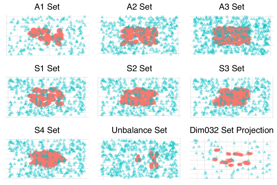
Figure 2: The eight benchmark datasets. Blue triangles represent added uniform noise.

Just like in Fränti and Yang (2018), we set the proportion of outliers at 7%. We generate uniform noise in each dimension in the range $[x_{\text{mean}}-2\times\text{range},x_{\text{mean}}+2\times\text{range}]$, where the range is the difference between the farthest observation and the mean in each dimension.

We run the OCLUST algorithm (Clark and McNicholas, 2022) in R, fixing the upper bound $F$ from Table 1, or about 10% of the original data size. We eliminate initial gross outliers with large Mahalanobis distances to regions of high density identified by the dbscan package (Hahsler et al., 2019). Variance structures for the S sets, A sets, and Unbalance set are unrestricted, allowing varying volumes, shapes, and orientations among the clusters. We restrict the Dim032 set to a variance structure with varying volumes and spherical shapes to hasten computation time. We run CNMix using the CNmixt function (Punzo et al., 2018) with default $k$-means initialization. The package chooses the best model for variance and contamination using the BIC. We run NCM using the Mclust function (Scrucca et al., 2016), initializing the noise component as a random sample of points with probability 1/4. We let the package choose the best model regarding variance structure. We run mean-shift outlier detection in Python using Yang ’s code. We specify the number of clusters and perform three iterations. Due to its superior performance in Fränti and Yang (2018), non-outlying points are clustered using random swap clustering in Python (Yang et al., 2021; Fränti, 2018) and run for the recommended 5000 iterations. We implement the DCSCAN algorithm with the dbscan package, setting the minimum number of points per cluster to be 20, and letting the package determine epsilon. For the thresholding approach, we calculate Mahalanobis distance from the centre of the dataset and trim those that are larger than the mean+3*sd. The remaining points are clustered with the mixture package.

We evaluate each method using three metrics: adjusted Rand index (ARI) (Hubert and Arabie, 1985), normalized mutual information (NMI) (Kvalseth, 1987), and centroid index (CI) (Fränti et al., 2014). The ARI is a measure of agreement between two partitions, e.g., between predicted clusters and true classes. The ARI ranges from 0 to 1, with 1 reflecting perfect agreement and 0 reflecting a random partition. Normalized mutual information is a measure of the amount of information shared between the true classes and the clustering solution. It is a scale from 0 to 1, with 0 corresponding to no mutual information and 1 corresponding to perfect agreement. Centroid index is a measure of dissimilarity among cluster centroids. It identifies the number of centroids which are incorrectly located. $\text{CI}=0$ reflects one-to-one correspondence between the estimated cluster centres and the ground truth. We calculate ARI and NMI for cluster agreement taking into account if points are classified into the correct group, considering outliers as one of those groups. We also apply ARI and NMI on the binary outlier classification only to identify whether poor performance can be attributed to poor outlier detection or poor classification. The results are shown in Table 2, with the best algorithm for each metric bolded.

Table 2: Results of the six outlier algorithms on the benchmark datasets. BinARI and BinNMI represent ARI and NMI calculated based on the outlier classification only.

A1 Set
Algorithm	ARI	BinARI	NMI	BinNMI	CI
OCLUST	0.96	0.92	0.97	0.80	0
Mean-Shift	0.97	0.88	0.98	0.74	0
2T	0.84	0.79	0.92	0.59	1
CNMix	0.74	0.00	0.86	0.00	5
NCM	0.79	0.87	0.89	0.71	3
DBSCAN	0.01	0.91	0.06	0.78	19

A2 Set
Algorithm	ARI	BinARI	NMI	BinNMI	CI
OCLUST	0.95	0.88	0.97	0.73	0
Mean-Shift	0.94	0.82	0.97	0.64	0
2T	0.81	0.78	0.93	0.59	4
CNMix	0.72	0.00	0.89	0.00	7
NCM	0.55	0.71	0.75	0.50	17
DBSCAN	0.00	0.81	0.04	0.63	34

A3 Set
Algorithm	ARI	BinARI	NMI	BinNMI	CI
OCLUST	0.94	0.88	0.97	0.73	0
Mean-Shift	0.93	0.81	0.97	0.63	0
2T	0.84	0.77	0.95	0.57	4
CNMix	0.72	0.00	0.90	0.00	11
NCM	0.53	0.67	0.76	0.45	26
DBSCAN	-0.00	0.78	0.04	0.58	49

S1 Set
Algorithm	ARI	BinARI	NMI	BinNMI	CI
OCLUST	0.96	0.88	0.96	0.74	0
Mean-Shift	0.95	0.84	0.96	0.69	0
2T	0.95	0.81	0.96	0.62	0
CNMix	0.80	0.00	0.87	0.00	2
NCM	0.90	0.87	0.93	0.71	1
DBSCAN	0.01	-0.07	0.18	0.03	0

S2 Set
Algorithm	ARI	BinARI	NMI	BinNMI	CI
OCLUST	0.91	0.87	0.92	0.72	0
Mean-Shift	0.92	0.88	0.93	0.73	0
2T	0.70	0.82	0.83	0.64	1
CNMix	0.72	0.07	0.82	0.01	3
NCM	0.86	0.87	0.90	0.71	1
DBSCAN	0.01	-0.07	0.13	0.02	2

S3 Set
Algorithm	ARI	BinARI	NMI	BinNMI	CI
OCLUST	0.72	0.85	0.79	0.69	0
Mean-Shift	0.71	0.81	0.78	0.64	0
2T	0.42	0.82	0.67	0.64	1
CNMix	0.54	0.00	0.69	0.00	4
NCM	0.55	0.86	0.72	0.69	3
DBSCAN	0.01	-0.06	0.07	0.02	9

S4 Set
Algorithm	ARI	BinARI	NMI	BinNMI	CI
OCLUST	0.42	0.78	0.65	0.58	1
Mean-Shift	0.63	0.83	0.72	0.68	0
2T	0.16	0.86	0.50	0.70	1
CNMix	0.40	0.00	0.59	0.00	4
NCM	0.56	0.87	0.69	0.71	2
DBSCAN	0.01	-0.07	0.11	0.02	8

Unbalance Set
Algorithm	ARI	BinARI	NMI	BinNMI	CI
OCLUST	1.00	0.96	0.99	0.90	0
Mean-Shift	0.43	0.47	0.58	0.30	5
2T	0.88	0.79	0.85	0.61	3
CNMix	0.99	0.00	0.94	0.00	3
NCM	0.99	0.94	0.96	0.84	2
DBSCAN	0.98	0.69	0.91	0.48	0

Dim032 Set
Algorithm	ARI	BinARI	NMI	BinNMI	CI
OCLUST	0.99	0.97	0.99	0.91	0
Mean-Shift	1.00	0.99	1.00	0.97	0
2T	0.71	1.00	0.87	1.00	4
CNMix	0.07	-0.03	0.38	0.04	1
NCM	0.98	0.93	0.99	0.82	0
DBSCAN	0.00	0.00	0.00	0.00	15

OCLUST does better than its competitors as the number of clusters increases (A2 and A3). OCLUST and mean-shift have $\text{CI}=0$ for all but one dataset. Mean-shift performs better than the Gaussian model-based approaches as the clusters become highly overlapped in S4. This is likely due to its distance-based clustering algorithm. The model-based approaches cannot recover symmetrical Gaussian distributions for each component when the data severely overlap. OCLUST and mean-shift attain similar results on the A1, S1, S2, and S3 datasets. Mean-shift performs well as expected for those sets because the clusters are spherical and separated, features which distanced-based clustering methods favour.

OCLUST, mean-shift, and NCM perform very well on the 32-dimensional dataset, likely due to the uniform generation of outliers. As the dimensionality increases, it is more likely for an outlier to be far from the clusters in any one direction. All of the simultaneous clustering/outlier detection algorithms perform well on the unbalanced dataset, Mean-shift filters most of the unbalanced points as noise, resulting in poor classification. DBSCAN performs poorly on most datasets, often over-specifying the number of outliers and combining clusters together. The thresholding approach performs consistently for outlier identification but fails when clusters become more overlapped, likely due to remaining outliers reducing clustering performance.

In Figure 3, the KL graph for the A3 dataset is plotted. It displays a typical shape, decreasing to a minimum at 446 outliers, after which KL increases. The minimum at 446 is notably different from 525, the number of outliers generated. However, this is to be expected due to the uniform generation of outliers; many of them overlap with the clusters as seen in Figure 2. All of the algorithms experience the same issue in this respect.

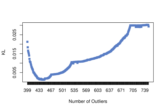
Figure 3: KL plot for the A3 dataset, where the minimum is at 446 outliers.

In the initial gross outlier removal for the A3 dataset, 399 outliers are removed. We reach a minimum KL divergence after 48 iterations, but continuing until $F=750$ requires a further 304 iterations. At the minimum KL, we achieve an approximate p-value of 0.099 on the Kuiper test when $B=100$. If our required p-value was 0.05, we would be able to stop here and save most of the computation time.

3.2 Crabs Study

Next we evaluate the sensitivity of OCLUST using the crabs dataset (Campbell and Mahon, 1974). This study closely mimics the study carried out by Peel and McLachlan (2000) and again by Punzo and McNicholas (2016) to demonstrate their respective approaches to dealing with outliers in model-based clustering.

The dataset contains observations for 100 blue crabs, 50 of which are male, and 50 of which are female. The aim for each classification is to recover the sex of the crab. For this study, we will focus on measurements of rear width (RW) and carapace length (CL). We substitute the CL value of 25th point to one of eight values in $[-15,20]$. The leftmost plot in Figure 4 plots the crabs dataset by sex, with the permuted value in red taking value $\text{CL}=-5$. We use the OCLUST, mean-shift, CNMix, NCM, and DBSCAN algorithms, along with the thresholding approach. For OCLUST, CNMix and NCM, we run each method, restricting the model to one where the clusters have equal shapes and volumes but varying orientations. We let the R package determine whether or not the CNMix model was contaminated. Solutions for OCLUST, CNMix, NCM, and the thresholding approach (2T) for the dataset with $\text{CL}=-5$ are plotted in Figure 4. Table 3 summarizes the results for each method, listing the number of misclassified points (M) and the predicted number of outliers ($n_{O}$).

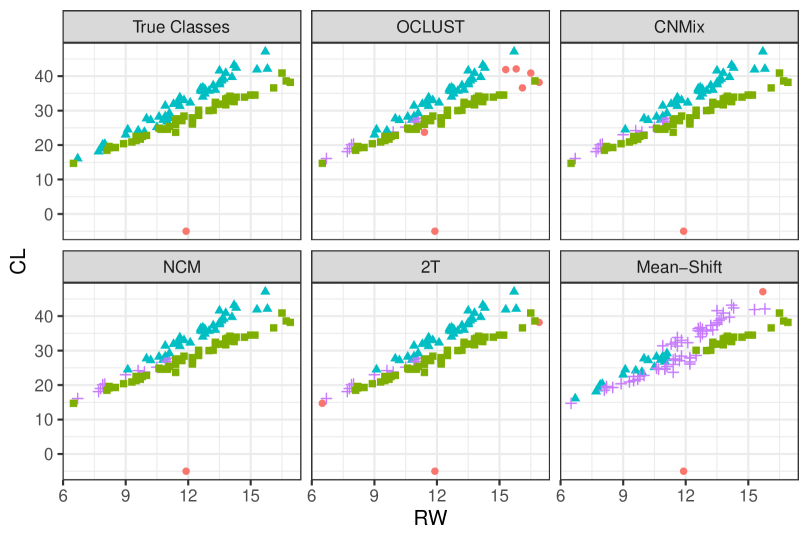
Figure 4: Predicted classifications for OCLUST, CNMix, NCM, mean-shift, and the thresholding approach (2T) when $\text{CL}=-5$. Green squares, blue triangles, purple crosses, and red circles indicate female, male, misclassified, and outlying points, respectively.

Table 3: Results for running each method on the crabs dataset, where ‘M’ and ‘$n_{O}$’ designate the number of misclassified points and number of predicted outliers, respectively.

	OCLUST			Mean-Shift			2T			CNMix			NCM			DBSCAN
CL	M	$n_{O}$		M	$n_{O}$		M	$n_{O}$		M	$n_{O}$		M	$n_{O}$		M	$n_{O}$
$-15$	11	8		41	3		12	4		13	1		13	1		50	0
$-10$	11	6		41	3		13	3		13	1		13	1		50	0
$-5$	11	7		41	3		13	3		13	1		13	1		50	0
0	11	4		41	3		13	2		13	1		13	1		50	0
5	12	5		41	3		13	3		13	1		13	2		50	0
10	11	4		41	3		13	3		13	1		11	3		50	0
15	11	5		41	3		13	3		13	1		10	4		50	0
20	11	5		42	2		14	4		13	1		9	5		50	0

Each method with the exception of DBCAN always identifies the permuted value correctly as an outlier. DBSCAN clusters all the data, including the outlier, into one cluster. NCM classifies more points as outliers as the permuted CL value becomes less extreme. In contrast, OCLUST does the reverse because when the outlier is farther away, it is removed in the gross outlier stage. It does not affect the initial clustering, allowing the algorithm to remove more points that diverge from multivariate normality.

OCLUST identifies more points as outliers than its competitors and has fewer misclassifications in most instances. It is important to note that OCLUST’s outliers are not NCM’s misclassifications. Instead, as seen in Figure 4, OCLUST identifies three points between the clusters as technical outliers. This removes the points with high leverage, allowing the clusters to rotate and improve the classification among low values of RW. There are likely a few more outliers identified than needed for classification sake, but their removal improves the model and its parameter estimates. The thresholding approach cannot identify technical outliers because it detects outliers before clustering. Mean shift performs poorly for this dataset due to the elliptical shape of the clusters.

3.3 Wine Data

Finally, we evaluate the results of OCLUST on the wine dataset, available in the gclus R package (Hurley, 2019). This dataset describes 13 attributes of 178 Italian wines (e.g., alcohol, hue, malic acid). Each wine originates from one of three cultivars. For this analysis, we add 12 points of noise, uniformly distributed in each dimension as described in Section 3.1. We perform unsupervised classification on this dataset with the aim of removing the noise and recovering the cultivar for each wine. We run OCLUST as well as the five other comparable methods in Section 3.2. The Gaussian methods are restricted to three clusters with a ‘VVI’ variance structure. The results for the competitor algorithms except DBSCAN are provided in Table 4. DBSCAN perfoms poorly by classifying all points into one cluster and only identifying seven points of added noise.

Table 4: Classification results for CNMix, NCM, 2T, mean-shift and OCLUST on the wine dataset. Classification results on the wine dataset for OCLUST at global minimum KL and when stopped when the p-value exceeds 0.05.

	CNMix					NCM					2T
Cultivar	1	2	3	bad		1	2	3	bad		1	2	3	bad
Barbera	40			8		47			1		48
Barolo		50		9			58	1				59
Grignolio	1	30		40		3	2	65	1		5	1	65
Noise			10	2					12					12
	Mean-Shift					OCLUST Min. KL					OCLUST p-val>0.05
Cultivar	1	2	3	bad		1	2	3	bad		1	2	3	bad
Barbera	29		19			34			14		45			3
Barolo	13	44		2			42		17			53		6
Grignolio	19	1	50	1				33	38		2		52	17
Noise	1			11					12					12

NCM achieves good results, with only six misclassifications, five of which are from the Grignolio class. It identifies all 12 points of added noise as outliers. CNMix classifies the noise into its own cluster and puts some of the Grignolio wines into the Barolo cluster and treats 40 as outliers. The thresholding approach performs very well, likely due to the uniform simulation of noise in 13 dimensions creating gross outliers. Mean-shift performs poorly, highlighting the shortcoming of distance-based clustering methods on oblong clusters.

The ideal solution for OCLUST, using the global minimum KL divergence is shown in Table 4. We have perfect classification among the good points, but 81 points are treated as outliers, which represents 43% of the dataset. Our KL graph in Figure 5(a) has two local minima, suggesting a nearly as good alternative solution with fewer outliers. We re-run the algorithm with our p-value stopping criterion and stop the algorithm at 38 outliers. The classification results with 38 outliers are shown in Table 4. This allows for the preservation of more original data with minimal decrease in classification accuracy.

The associated KL plot (Figure 5) displays a pattern unlike Figure 3 because the data are real and not perfectly multivariate normal. We test each cluster for multivariate normality when all 81 outliers are removed and at the intermediate solution with 38 outliers. We test the null hypothesis of multivariate normality using the Energy Test in the energy package (Székely and Rizzo, 2013; Rizzo and Székely, 2022). When 38 outliers are removed, the Barolo, Barbera, and Grignolio clusters have p-values of 0.15, 0.11, and 0.20 respectively. At the optimal solution with 78 points removed, the Barolo, Barbera, and Grignolio clusters have p-values of 0.93, 0.79, and 0.30 respectively. Evidently, OCLUST continues to remove points until the clusters are unmistakably multivariate normal. One may choose to stop the algorithm early for specific clustering results or continue until the clusters are ideal to obtain more robust parameter estimates.

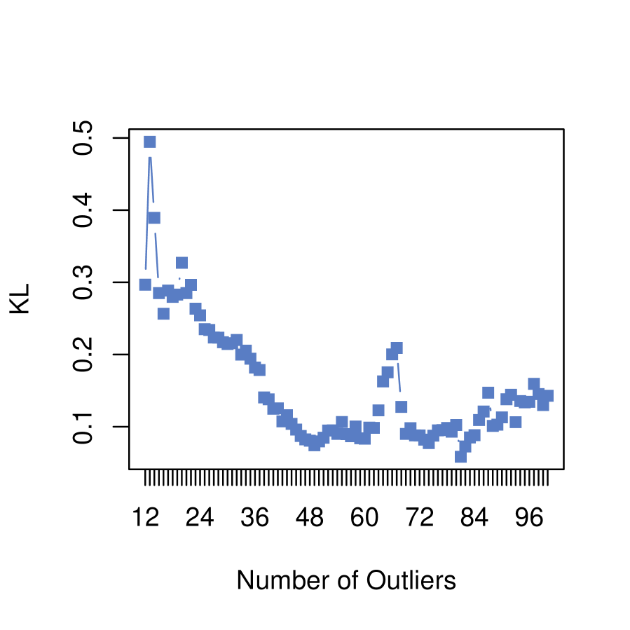
(a) KL plot for the wine dataset. The algorithm is run to an upper bound of 100 outliers.

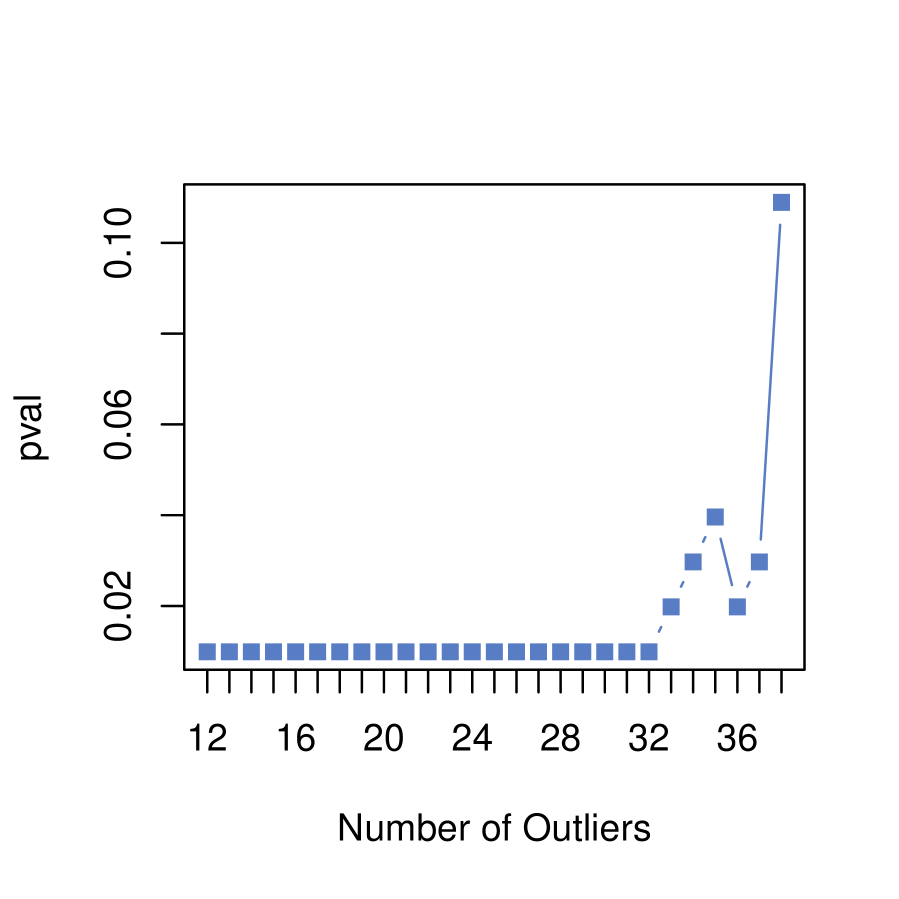
(b) p-value plot for the wine dataset. The algorithm is stopped at 38 outliers because the p-value is greater than 0.05

Figure 5: KL and p-value plots, respectively, for the wine dataset.

A two-dimensional projection of both OCLUST solutions are shown in Figure 6. In the left-hand figure where only 38 points are removed, we see some of the outliers are far from the clusters, but many of the bad points are technical outliers. Although they are not extreme in either direction, they fall outside of the clusters’ variance structure. In the right-hand plot, we see the solution when more points are removed. Although they may have been correctly classified, they deviate from the symmetrical ovoid shape characteristic of the multivariate normal distribution. The competing Gaussian classification algorithms are able to correctly cluster these points, but they seem not to fit well within the model. Identifying these additional outliers may be useful in novelty detection. These wines present inconsistent features which may be relevant to quality control. The spurious points do not fit into the model and indicate wines with chemical and physical properties that differ from the rest.

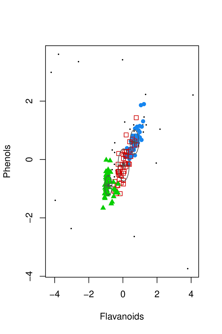
(a) Noisy wine dataset with 38 points removed.

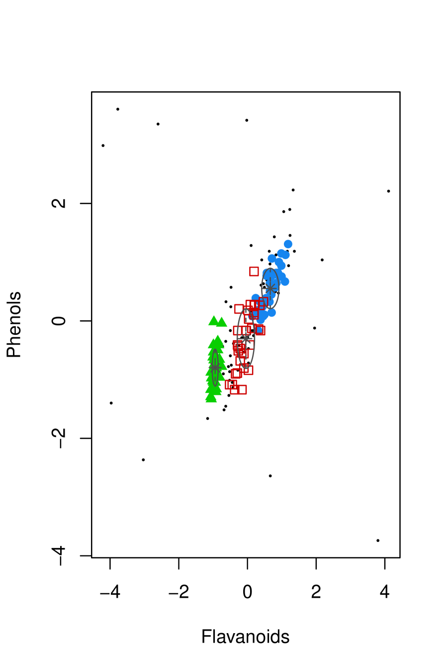
(b) Noisy wine dataset with 81 points removed.

Figure 6: Predicted classifications by OCLUST for the noisy wine dataset. The data are plotted in two dimensions, showing measurements for Flavanoids and Phenols. Small black points are the predicted outliers.

4 Discussion

It was shown that, for data from a Gaussian mixture, the log-likelihoods of the subset models are approximately distributed according to a mixture of beta distributions. This result was used to identify outliers without needing to specify their proportion by removing outlying points until the subset log-likelihoods followed this derived distribution. The result is the OCLUST algorithm, which trims outliers from a dataset while clustering using Gaussian mixture models. In simulations, OCLUST performs similarly or better than mean-shift outlier detection in most benchmark datasets except where there is extreme overlap. It performs similarly to noise component mixtures when the clusters are elliptical in the real datasets. Thus, it performs consistently well in both cases, when its competitors are best suited in one domain. In the crabs study, OCLUST trims technical outliers with high leverage, which improves the classification among small values of carapace length. On the wine data, OCLUST obtains good classification at low iterations. If the algorithm is allowed to continue, it removes points which deviate from the assumption of multivariate normality, possibly removing too many points in the process.

Although this work used the distribution of the log-likelihoods of the subset models to test for the presence of outliers, the derived distribution may be used to verify other underlying model assumptions, such as whether the clusters are Gaussian. Note that the OCLUST algorithm could be used with other clustering methods and should be effective so long as is it reasonable to assume that the underlying distribution of clusters is Gaussian. Of course, one could extend this work by deriving the distribution of subset log-likelihoods for mixture models with non-Gaussian components. This would allow direct consideration of asymmetric clusters with outliers. Finally, this model is limited by dimensionality because without sufficient observations, the underlying mixture model becomes over parametrized. One could extend this approach to high-dimensional data by using an analogue of the mixture of factor analyzers model or its extensions (see Ghahramani and Hinton (1997), McNicholas and Murphy (2008), McNicholas and Murphy (2010)). Based on the comparisons conducted herein, one might expect the resulting method to perform favourably, or at least comparably, when compared to the approaches used by Wei and Yang (2012) and Punzo et al. (2020).

Acknowledgments

This work was supported by an NSERC Undergraduate Research Award, an NSERC Canada Graduate Scholarship, the Canada Research Chairs program, and an E.W.R. Steacie Memorial Fellowship.

Appendix A Relaxing Assumptions

Lemma 1 assumes that the clusters are well separated and non-overlapping to simplify the model density to the component density. This section, however, serves to show that this assumption may be relaxed in practice. Following Qiu and Joe (2006), we can quantify the separation between clusters using the separation index $J^{*}$; in the univariate case,

$$J^{*}=\frac{L_{2}(\alpha/2)-U_{1}(\alpha/2)}{U_{2}(\alpha/2)-L_{1}(\alpha/2)},$$

where $L_{i}(\alpha/2)$ is the sample lower $\alpha/2$ quantile and $U_{i}(\alpha/2)$ is the sample upper $\alpha/2$ quantile of cluster $i$, and cluster 1 has lower mean than cluster 2. In the multivariate case, the separation index is calculated along the projected direction of maximum separation. Clusters with $J^{*}>0$ are separated, clusters with $J^{*}<0$ overlap, and clusters with $J^{*}=0$ are touching.

To measure the effect of separation index on the approximate log-likelihood $Q_{\mathcal{X}}$, 100 random datasets with $n=1800$ for each combination were generated using the clusterGeneration (Qiu and Joe, 2015) package in R. Data were created with three clusters with equal cluster proportions with dimensions $p\in\{2,4,6\}$ and separation indices in $[-0.9,0.9]$. Covariance matrices were generated using random eigenvalues $\lambda\in[0,10]$. The parameters were estimated using the EM algorithm. The log-likelihoods using the full and approximate densities were calculated using the parameter estimates. $[Q_{\mathcal{X}}-\ell_{\mathcal{X}}]/\ell_{\mathcal{X}}$, the average proportional change in log-likelihood over the 100 datasets between the full log-likelihood $\ell_{\mathcal{X}}$ and the approximate log-likelihood $Q_{\mathcal{X}}$, is shown in Figure 7.

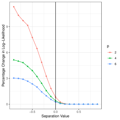
Figure 7: The effect of cluster separation on the approximate log-likelihood of the model, where the vertical line represents the threshold between separated and overlapping clusters.

As one would expect, the approximation of $\ell_{\mathcal{X}}$ by $Q_{\mathcal{X}}$ improves as the separation index increases (see Lemma 1). However, the difference is negligible for touching and separated clusters ($J^{*}\geq 0$).

Appendix B Mathematical Results

B.1 Proof of Lemma 1

Proof.

Suppose $\mathbf{\Sigma}$ is positive definite. Then, $\mathbf{\Sigma}^{-1}$ is also positive definite and there exists $\mathbf{Q}^{\prime}\mathbf{Q}=\mathbf{I}$ such that $\mathbf{\Sigma}^{-1}=\mathbf{Q}^{\prime}\mathbf{\Lambda}\mathbf{Q}$ and $\mathbf{\Lambda}$ is diagonal with $\mathbf{\Lambda}_{ii}=\lambda_{i}>0,i\in[1,p]$. Let $\mathbf{x}-\boldsymbol{\mu}=\mathbf{Q}^{\prime}\mathbf{w}$, where $\mathbf{w}\neq\mathbf{0}$. Now,

$$\begin{split}(\mathbf{x}-\boldsymbol{\mu})^{\prime}\mathbf{\Sigma}^{-1}(\mathbf{x}-\boldsymbol{\mu})&=\mathbf{w}^{\prime}\mathbf{Q}\mathbf{\Sigma}^{-1}\mathbf{Q}^{\prime}\mathbf{w}=\mathbf{w}^{\prime}\mathbf{\Lambda}\mathbf{w}=\sum_{i=1}^{p}\lambda_{i}w_{i}^{2}\\ &\geq\inf_{i}(\lambda_{i})\sum_{i=1}^{p}w_{i}^{2}=\inf_{i}(\lambda_{i})\|\mathbf{w}\|^{2}=\inf_{i}(\lambda_{i})\|\mathbf{x}-\boldsymbol{\mu}\|^{2}\end{split}$$

because $\|\mathbf{x}-\boldsymbol{\mu}\|^{2}=\|\mathbf{Q}^{\prime}\mathbf{w}\|^{2}=\mathbf{w}^{\prime}\mathbf{Q}\mathbf{Q}^{\prime}\mathbf{w}=\|\mathbf{w}\|^{2}$. Thus, as $\|\mathbf{x}-\boldsymbol{\mu}\|\rightarrow\infty,(\mathbf{x}-\boldsymbol{\mu})^{\prime}\mathbf{\Sigma}^{-1}(\mathbf{x}-\boldsymbol{\mu})\rightarrow\infty$ and

$$\phi(\mathbf{x}\mid\boldsymbol{\mu},\mathbf{\Sigma})=\frac{1}{\sqrt{(2\pi)^{p}|\mathbf{\Sigma}|}}\text{exp}\left\{-\frac{1}{2}(\mathbf{x}-\boldsymbol{\mu})^{\prime}\mathbf{\Sigma}^{-1}(\mathbf{x}-\boldsymbol{\mu})\right\}\rightarrow 0.$$

Suppose $\mathbf{x}_{i}\in\mathcal{C}_{h}$. Then, as the clusters separate, $\|\mathbf{x}_{i}-\boldsymbol{\mu}_{g}\|\rightarrow\infty$ and $\phi(\mathbf{x}_{i}\mid\boldsymbol{\mu}_{g},\mathbf{\Sigma}_{g})\rightarrow 0$ for $g\neq h$. Thus, for $\mathbf{x}_{i}\in\mathcal{C}_{h}$,

$$\begin{split}\sum_{g=1}^{G}\pi_{g}\phi(\mathbf{x}_{i}\mid\boldsymbol{\mu}_{g},\mathbf{\Sigma}_{g})&=\sum_{g\neq h}\pi_{g}\phi(\mathbf{x}_{i}\mid\boldsymbol{\mu}_{g},\mathbf{\Sigma}_{g})+\pi_{h}\phi(\mathbf{x}_{i}\mid\boldsymbol{\mu}_{h},\mathbf{\Sigma}_{h})\simeq\pi_{h}\phi(\mathbf{x}_{i}\mid\boldsymbol{\mu}_{h},\mathbf{\Sigma}_{h}).\end{split}$$

Thus,

$$\begin{split}\ell_{\mathcal{X}}&=\sum_{i=1}^{n}\log\left[\sum_{g=1}^{G}\pi_{g}\phi(\mathbf{x}_{i}\mid\boldsymbol{\mu}_{g},\mathbf{\Sigma}_{g})\right]\simeq\sum_{\mathbf{x}_{i}\in\mathcal{C}_{g}}\log\left[\pi_{g}\phi(\mathbf{x}_{i}\mid\boldsymbol{\mu}_{g},\mathbf{\Sigma}_{g})\right]=Q_{\mathcal{X}}.\end{split}$$

∎

Remark 4.

Although covariance matrices need only be positive semi-definite, we restrict $\mathbf{\Sigma}$ to be positive definite so that $\mathbf{X}$ is not degenerate.

Appendix C Computation Time

Table 5 records the computation time in seconds for each algorithm. The entire OCLUST algorithm is timed without the p-value stopping criterion. The mean-shift algorithm is run in Python with 5000 random swaps. All other algorithms are run in R. Competing algorithms are run in series on a cluster with Intel Xeon Silver 4114 CPUs. The OCLUST algorithm was run on that same cluster for all datasets except Dim032. The benchmark and crabs sets were run in parallel with 80 cores and wine was run with 20. Dim032 was run with 30 cores on a separate cluster of Intel Xeon E5-4627 v2 CPUs.

Table 5: Computation time in seconds for each outlier algorithm on all datasets.

Dataset	Full OCLUST	Mean-Shift	2T	CNMix	NCM	DBSCAN
A1	5.89E+03	2.98E+04	2.38E+02	2.77E+02	6.14E+00	2.92E-01
A2	3.95E+04	6.42E+04	7.29E+02	1.44E+02	9.86E+00	2.46E-01
A3	6.41E+04	2.01E+05	2.11E+03	5.16E+03	3.71E+01	4.70E-01
S1	1.01E+04	4.28E+04	1.15E+02	1.84E+02	6.76E+00	2.69E-01
S2	1.85E+04	4.06E+04	2.14E+02	3.06E+02	1.03E+01	2.60E-01
S3	6.43E+04	3.13E+04	2.86E+02	3.50E+02	1.96E+01	3.07E-01
S4	1.37E+05	2.47E+04	3.60E+02	4.65E+02	2.19E+01	2.22E-01
Unbalance	9.93E+05	1.96E+04	3.80E+02	1.26E+02	5.53E+00	5.67E-01
Dim032	7.35E+03	8.566E+03	2.28E+02	1.55E+03	7.71E+01	3.05E-01
Wine	1.09E+02	1.80E+02	2.38E+02	4.79E-01	2.47E-01	7.09E-02
Crabs (avg.)	3.75E+00	1.06E+02	2.93E-02	9.02E-01	9.66E-02	3.66E-02

References

- Banfield and Raftery (1993) Banfield, J. D. and A. E. Raftery (1993). Model-based Gaussian and non-Gaussian clustering. Biometrics 49(3), 803–821.
- Boukerche et al. (2020) Boukerche, A., L. Zheng, and O. Alfandi (2020). Outlier detection: Methods, models, and classification. ACM Computing Surveys (CSUR) 53(3), 1–37.
- Buzzi-Ferraris and Manenti (2011) Buzzi-Ferraris, G. and F. Manenti (2011). Outlier detection in large data sets. Computers & Chemical Engineering 35(2), 388–390.
- Campbell and Mahon (1974) Campbell, N. A. and R. J. Mahon (1974). A multivariate study of variation in two species of rock crab of genus leptograpsus. Australian Journal of Zoology 22, 417–425.
- Clark and McNicholas (2022) Clark, K. M. and P. D. McNicholas (2022). oclust: Gaussian Model-Based Clustering with Outliers. R package version 0.2.0.
- Cuesta-Albertos et al. (1997) Cuesta-Albertos, J. A., A. Gordaliza, and C. Matrán (1997, 04). Trimmed -means: an attempt to robustify quantizers. The Annals of Statistics 25(2), 553–576.
- Dempster et al. (1977) Dempster, A. P., N. M. Laird, and D. B. Rubin (1977). Maximum likelihood from incomplete data via the EM algorithm. Journal of the Royal Statistical Society: Series B 39(1), 1–38.
- Domingues et al. (2018) Domingues, R., M. Filippone, P. Michiardi, and J. Zouaoui (2018). A comparative evaluation of outlier detection algorithms: Experiments and analyses. Pattern Recognition 74, 406–421.
- Ester et al. (1996) Ester, M., H.-P. Kriegel, J. Sander, and X. Xu (1996). A density-based algorithm for discovering clusters in large spatial databases with noise. pp. 226–231. AAAI Press.
- Fränti (2018) Fränti, P. (2018). Efficiency of random swap clustering. Journal of Big Data 5(1), 13.
- Fränti et al. (2014) Fränti, P., M. Rezaei, and Q. Zhao (2014). Centroid index: Cluster level similarity measure. Pattern Recognition 47(9), 3034–3045.
- Fränti and Sieranoja (2018) Fränti, P. and S. Sieranoja (2018). K-means properties on six clustering benchmark datasets. Applied Intelligence 48(12), 4743–4759.
- Fränti and Yang (2018) Fränti, P. and J. Yang (2018). Medoid-shift for noise removal to improve clustering. In International Conference on Artificial Intelligence and Soft Computing, pp. 604–614. Springer.
- García-Escudero et al. (2008) García-Escudero, L. A., A. Gordaliza, C. Matrán, and A. Mayo-Iscar (2008). A general trimming approach to robust cluster analysis. The Annals of Statistics 36(3), 1324–1345.
- Ghahramani and Hinton (1997) Ghahramani, Z. and G. E. Hinton (1997). The EM algorithm for factor analyzers. Technical Report CRG-TR-96-1, University of Toronto, Toronto, Canada.
- Gnanadesikan and Kettenring (1972) Gnanadesikan, R. and J. R. Kettenring (1972). Robust estimates, residuals, and outlier detection with multiresponse data. Biometrics 28(1), 81–124.
- Grubbs (1969) Grubbs, F. E. (1969). Procedures for detecting outlying observations in samples. Technometrics 11(1), 1–21.
- Hahsler et al. (2019) Hahsler, M., M. Piekenbrock, and D. Doran (2019). dbscan: Fast density-based clustering with R. Journal of Statistical Software 91(1), 1–30.
- Hampel (1974) Hampel, F. R. (1974). The influence curve and its role in robust estimation. Journal of the American Statistical Association 69(346), 383–393.
- Hautamäki et al. (2005) Hautamäki, V., S. Cherednichenko, I. Kärkkäinen, T. Kinnunen, and P. Fränti (2005). Improving k-means by outlier removal. In Scandinavian Conference on Image Analysis, pp. 978–987. Springer.
- Hubert and Arabie (1985) Hubert, L. and P. Arabie (1985). Comparing partitions. Journal of Classification 2(1), 193–218.
- Hurley (2019) Hurley, C. (2019). gclus: Clustering Graphics. R package version 1.3.2.
- Knorr and Ng (1998) Knorr, E. M. and R. T. Ng (1998). Algorithms for mining distance-based outliers in large datasets. In VLDB, Volume 98, pp. 392–403. Citeseer.
- Kuiper (1960) Kuiper, N. H. (1960). Tests concerning random points on a circle. In Nederl. Akad. Wetensch. Proc. Ser. A, Volume 63, pp. 38–47.
- Kvalseth (1987) Kvalseth, T. O. (1987). Entropy and correlation: Some comments. IEEE Transactions on Systems, Man, and Cybernetics 17(3), 517–519.
- Liu et al. (2019) Liu, Y., Z. Li, C. Zhou, Y. Jiang, J. Sun, M. Wang, and X. He (2019). Generative adversarial active learning for unsupervised outlier detection. IEEE Transactions on Knowledge and Data Engineering 32(8), 1517–1528.
- McNicholas (2016) McNicholas, P. D. (2016). Model-based clustering. Journal of Classification 33(3), 331–373.
- McNicholas and Murphy (2008) McNicholas, P. D. and T. B. Murphy (2008). Parsimonious Gaussian mixture models. Statistics and Computing 18(3), 285–296.
- McNicholas and Murphy (2010) McNicholas, P. D. and T. B. Murphy (2010). Model-based clustering of microarray expression data via latent Gaussian mixture models. Bioinformatics 26(21), 2705–2712.
- North et al. (2002) North, B. V., D. Curtis, and P. C. Sham (2002). A note on the calculation of empirical p values from monte carlo procedures. The American Journal of Human Genetics 71(2), 439–441.
- Peel and McLachlan (2000) Peel, D. and G. J. McLachlan (2000). Robust mixture modelling using the t distribution. Statistics and Computing 10(4), 339–348.
- Pimentel et al. (2014) Pimentel, M. A. F., D. A. Clifton, L. Clifton, and L. Tarassenko (2014). A review of novelty detection. Signal Processing 99, 215–249.
- Pocuca et al. (2021) Pocuca, N., R. P. Browne, and P. D. McNicholas (2021). mixture: Mixture Models for Clustering and Classification. R package version 2.0.4.
- Punzo et al. (2020) Punzo, A., M. Blostein, and P. D. McNicholas (2020). High-dimensional unsupervised classification via parsimonious contaminated mixtures. Pattern Recognition 98, 107031.
- Punzo et al. (2018) Punzo, A., A. Mazza, and P. D. McNicholas (2018). ContaminatedMixt: An R package for fitting parsimonious mixtures of multivariate contaminated normal distributions. Journal of Statistical Software 85(10), 1–25.
- Punzo and McNicholas (2016) Punzo, A. and P. D. McNicholas (2016, 11). Parsimonious mixtures of multivariate contaminated normal distributions. Biometrical Journal 58(6), 1506–1537.
- Qiu and Joe (2006) Qiu, W. and H. Joe (2006). Separation index and partial membership for clustering. Computational Statistics & Data Analysis 50(3), 585–603.
- Qiu and Joe (2015) Qiu, W. and H. Joe (2015). clusterGeneration: Random Cluster Generation (with Specified Degree of Separation). R package version 1.3.4.
- R Core Team (2021) R Core Team (2021). R: A Language and Environment for Statistical Computing. Vienna, Austria: R Foundation for Statistical Computing.
- Ramaswamy et al. (2000) Ramaswamy, S., R. Rastogi, and K. Shim (2000). Efficient algorithms for mining outliers from large data sets. In Proceedings of the 2000 ACM SIGMOD international conference on Management of data, pp. 427–438.
- Rizzo and Székely (2022) Rizzo, M. and G. Székely (2022). energy: E-Statistics: Multivariate Inference via the Energy of Data. R package version 1.7-10.
- Scrucca et al. (2016) Scrucca, L., M. Fop, T. B. Murphy, and A. E. Raftery (2016). mclust 5: Clustering, classification and density estimation using Gaussian finite mixture models. The R Journal 8(1), 205–233.
- Székely and Rizzo (2013) Székely, G. J. and M. L. Rizzo (2013). Energy statistics: A class of statistics based on distances. Journal of Statistical Planning and Inference 143(8), 1249–1272.