Stochastic Lagrangians for Statistical Dynamics

Abstract

The concept of stochastic Lagrangian and its use in statistical dynamics is illustrated theoretically, and with some examples.

Dynamical variables undergoing stochastic differential equations are stochastic processes themselves, and their realization probability functional within a given time interval arises from the interplay between the deterministic parts of dynamics and noise statistics. The stochastic Lagrangian is a tool to formulate realization probabilities via functional integrals, once the statistics of noises involved in the stochastic dynamical equations is known. In principle, it allows to highlight the invariance properties of the statistical dynamics of the system.

In this work, after a review of the stochastic Lagrangian formalism, some applications of it to physically relevant cases are illustrated.

Keywords: Stochastic Dynamics, Action Principle, Functional Formalism, Path Integrals, Langevin Equation

Contents

1. 1 Introduction
2. 2 Functional Formalism for Statistical Dynamics
   1. 2.1 Stochastic Lagrangian
   2. 2.2 $\delta$-correlated Gaussian noise
3. 3 Examples
   1. 3.1 Point Particle with noise
   2. 3.2 Leibniz systems
      1. 3.2.1 Hamiltonian Systems
      2. 3.2.2 Metriplectic Systems
4. 4 Conclusions
5. A Calculation for § 2.2
   1. A.1 Calculation of $C\left[\chi,\Gamma;t_{\mathrm{i}},t_{\mathrm{f}}\right)$
   2. A.2 Calculation of $A\left[\psi,\chi;t_{\mathrm{i}},t_{\mathrm{f}}\right)$ and $\mathcal{A}\left[\psi;t_{\mathrm{i}},t_{\mathrm{f}}\right)$
6. B Calculations for § 3.1
   1. B.1 Calculation of the Stochastic Lagrangian
   2. B.2 Calculating $\mathcal{J}_{0}$ and $\mathcal{I}_{k}$
   3. B.3 Keeping $\tilde{N}_{0}\left(\zeta;t_{\mathrm{i}},t_{\mathrm{f}}\right)$ finite
7. C Calculations for § 3.2

Institute for Complex Systems of the National Research Council (CNR-ISC), Florence, Italy.
E-mail: massimo.materassi@isc.cnr.it, massimomaterassi27@gmail.com.
Web: www.materassiphysics.com.

1 Introduction

After Isaac Newton’s big work about “the motion of bodies” [1], it was understood that physical systems are generally governed by equations of motion, expressing the variability with time of the state of the system in terms of the state of what acts on the system. When one writes $\vec{F}=m\vec{a}$, the time variability $\frac{d\vec{p}}{dt}$ of “the state of motion” of the pointlike particle $\vec{p}$ (namely, its momentum) is put in relationship with “the force” $\vec{F}$ as

$$\frac{d\vec{p}}{dt}=\vec{F},$$ (1)

and this force is a function of the state of what acts on the system. As an example, think about Kepler’s problem, in which the point of mass $m$ at position $\vec{x}$ undergoes the gravitational force exerted by the presence of another body of mass $M$ at position $\vec{x}_{\odot}$, according to the law

$$\frac{d\vec{p}}{dt}=\frac{GMm}{\left|\vec{x}_{\odot}-\vec{x}\right|^{3}}\left(\vec{x}_{\odot}-\vec{x}\right):$$ (2)

the state of what acts on the pointlike particle is described indeed by the force $\vec{F}=\frac{GMm}{\left|\vec{x}_{\odot}-\vec{x}\right|^{3}}\left(\vec{x}_{\odot}-\vec{x}\right)$, containing the value of the gravitational mass $M$ of the second body and its relative position with respect to the point particle of momentum $\vec{p}$, i.e. $\vec{x}_{\odot}-\vec{x}$. By the way, notice that in the force the state of the system itself appears as $\vec{x}$, rendering (1) and (2) proper differential equations for the state of the system $\psi=\left(\vec{x},\vec{p}\right)$. As Newton’s equation $\vec{F}=m\vec{a}$ is re-written considering also the relationship between momentum and velocity, one writes

$$\begin{cases}&\dfrac{d\vec{x}}{dt}=\dfrac{\vec{p}}{m},\\ \\ &\dfrac{d\vec{p}}{dt}=\vec{F}\left(\vec{x},\vec{p},t,X_{\mathrm{env}}\right):\end{cases}$$ (3)

here it is stressed that the “force” is a function of the system state, of time $t$ and of the “state of the environment” acting on the system, indicated as $X_{\mathrm{env}}$. A system as (3) is properly a system of ordinary differential equations (ODE), in which the variability of the state $\psi$, of the portion of universe we are intersted in, is put in relationship with how this portion of universe interacts with the environment. Similar systems of ODEs may be written as:

$$\dfrac{d\psi}{dt}=\varphi\left(\psi,t,X_{\mathrm{env}}\right).$$ (4)

In such a formulation, the system is described by a state $\psi\in\mathbb{V}$, where $\mathbb{V}$ is a certain mathematical ambient through which the state $\psi$ moves as time flows; $\mathbb{V}$ is referred to as the phase space of the system.

Calculus teaches us that when ODEs as (4) are equipped with some initial condition $\psi\left(t_{0}\right)=\psi_{0}$, the problem

$$\begin{cases}&\dfrac{d\psi}{dt}=\varphi\left(\psi,t,X_{\mathrm{env}}\right),\\ \\ &\psi\left(t_{0}\right)=\psi_{0}\end{cases}$$ (5)

admits a unique solution $\psi\left(t\right)=\Psi_{\varphi}\left(t,\psi_{0}\right)$ for all $t\geq t_{0}$. To be honest, this happens only if the Cauchy Problem (5) has the expression $\varphi\left(\psi,t,X_{\mathrm{env}}\right)$ that has particularly favorable conditions with respect to $\psi$, which we assume to happen “always” (however, see [2] for a not-that-problematic counterexample). From here on, the statement

$$(\ref{eq:Cauchy.Problem})\thinspace\implies\thinspace\psi\left(t\right)=\Psi_{\varphi}\left(t,\psi\left(t_{0}\right)\right)\ \forall\ t\geq t_{0}$$ (6)

means that there exists a (suitably regular) map $\Psi_{\varphi}:\mathbb{R}\times\mathbb{V}\mapsto\mathbb{V}$ depending on the dynamics $\varphi$, associating the state $\psi\left(t\right)$ to the initial condition $\psi\left(t_{0}\right)$ in an injective way. This map $\Psi_{\varphi}$ is what one calls evolution. As a note, let us introduce here the system velocity space $\mathbb{W}$, or dynamical flow space, so that $\varphi\left(\psi,t,X_{\mathrm{env}}\right)\in\mathbb{W}$ and $\varphi:\mathbb{V}\times\mathbb{R}\times\mathbb{V}_{\mathrm{env}}\mapsto\mathbb{W}$ (here $\mathbb{V}_{\mathrm{env}}$ is the phase space of the environment acting on the system).

Uniqueness of the solution of initial value problems (5) nourishes the Deterministic Paradigm (DP), according to which once a system’s initial conditions are given, its future history will be completely determined, as long as what acts on it is known for all the future times. This is strongly accepted all through the Classical Physics, and after all it is true also in Quantum Mechanics [3], just considering the ODE (4) to be Schrödinger equation $i\hbar\frac{d}{dt}\left|\psi\right\rangle=H\left|\psi\right\rangle$, according to which the motion of the quantum state $\left|\psi\right\rangle$ is a perfectly deterministic trajectory through the quantum state Hilbert space $\mathbb{H}_{S}$.

The intelligent criticism to the DP (that actually turns out to be a generalization of the DP itself) must be based on the observation that, in order for (5) to have a unique solution, the quantities $X_{\mathrm{env}}$ and $\psi_{0}$ appearing there, and the full mathematical construction of $\varphi\left(\psi,t,X_{\mathrm{env}}\right)$, must be known perfectly, i.e. with no uncertainty.

For instance, as the initial condition $\psi_{0}$ is not known perfectly, instead one knows just $\psi_{0}$ to belong to some subset $A_{0}\subseteq\mathbb{V}$ of the phase space $\mathbb{V}$, as

$$\begin{cases}&\dfrac{d\psi}{dt}=\varphi\left(\psi,t,X_{\mathrm{env}}\right),\\ \\ &\psi\left(t_{0}\right)\in A_{0},\end{cases}$$ (7)

one must admit the state of the system at time $t\geq t_{0}$ to be any state $\Psi\left(t,\psi\left(t_{0}\right)\right)$ for any $\psi\left(t_{0}\right)\in A_{0}$, i.e.:

$$(\ref{eq:coarse.grained.initial.conditions})\thinspace\implies\thinspace\psi\left(t\right)\in\Psi_{\varphi}\left(t,A_{0}\right)\ \forall\ t\geq t_{0},$$

being $A_{0}$ a finite size set, and so the set $\Psi_{\varphi}\left(t,A_{0}\right)$. Put in a simpler way, with a coarse grained knowledge of the initial condition as $\psi\left(t_{0}\right)\in A_{0}$ instead of the sharp $\psi\left(t_{0}\right)=\psi_{0}$, one has to get content with a coarse grained knowledge of the state $\psi\left(t\right)$ at later times. The uncertainty in the initial conditions will render uncertain the evolution of the system, setting a natural limit to the DP due to our finite precision and to how fast a finite size initial condition set $A_{0}$ may be deformed by the dynamics in (5): the whole querelle between the DP and chaos theory comes precisely from the capacity of non-linear dynamics to deform the initial condition set $A_{0}$ and diffuse it all over extended and complicated regions of the phase space, rendering the evolution unpredictable to an arbitrarily high precision.

In this work we will examine a different “limit of the DP”: namely, we will deal with what happens when some elements of the mathematical expression of $\varphi$ are known only to some statistical extent, i.e. when this mathematical function of $\psi$, $t$ and $X_{\mathrm{env}}$ has terms whose exact values is unknown, and of which one can only state they appear according to some given probability distribution. As a simple example, consider $\psi$ to be a real variable, and the dynamics $\varphi$ to read

$$\varphi=K\psi^{2}+\gamma\left(t\right)\ /\ \gamma\left(t\right)\sim P_{t}:\Xi\mapsto\mathbb{R}^{+},\ \int_{\Xi}\mathcal{P}_{t}\left(\gamma\right)d\gamma=1,\ \forall\thinspace t>t_{0},$$ (8)

where $K$ is a coefficient, and the time-dependent term $\gamma\left(t\right)$ is an addendum that is “extracted from some real set $\Xi$” at each $t>t_{0}$, according to the probability distribution function $P_{t}$. A situation as that written in (8) represents the case in which the dynamics $\varphi$ is obtained, at each time, by a first “completely known” term $K\psi^{2}$ plus some term $\gamma$ about which one only knows that it can be a value within the set $\Xi$: as nothing sharper can be stated on $\gamma$, the value $\gamma\left(t\right)$ comes randomly within $\Xi$ at each different time, with a probability $P_{t}\left(\gamma^{*}\right)\delta$ to fall in any interval $\left[\gamma^{*}-\frac{\delta}{2},\gamma^{*}+\frac{\delta}{2}\right]$.

Terms as the $\gamma\left(t\right)$ in (8) are referred to as stochastic terms or, more simply, noises. In general, “noise terms” may appear in a variety of ways in the dynamics $\varphi$, due to different “physical” reasons: typically, as one distinguishes the dynamical variables $\psi$ assigning the state of the system from “everything else” encoded in $X_{\mathrm{env}}$, noise terms will sensibly describe the degree of uncertainty about $X_{\mathrm{env}}$, which is the other possible source of uncertainty in (5), next to the initial conditions. For instance, in (8) one might imagine that $\psi$ self-evolves with $K\psi^{2}$, and undergoes the action of the “random kicks” $\gamma$.

Considering that noise terms typically come from what one refers to as “environment”, the general form of (8) may read:

$$\varphi=\varphi\left(\psi,t,X_{\mathrm{env}}\left(\gamma\left(t\right)\right)\right)\ /\ \gamma\left(t\right)\sim P_{t}:\Xi\mapsto\mathbb{R}^{+},\ \int_{\Xi}P_{t}\left(\gamma\right)d\gamma=1,\ \forall\thinspace t>t_{0}.$$ (9)

In the presence of noise terms, the equation (4) is named stochastic dynamical equation (SDE). The stochastic version of (5) will read:

$$\begin{cases}&\dfrac{d\psi}{dt}=\varphi\left(\psi,t,X_{\mathrm{env}}\left(\gamma\left(t\right)\right)\right),\\ \\ &\psi\left(t_{0}\right)=\psi_{0},\\ \\ &\gamma\left(t\right)\sim P_{t}:\Xi\mapsto\mathbb{R}^{+}.\end{cases}$$ (10)

The most relevant fact passing from (5) to (10) is that the uniqueness of the solution is lost, even in the presence of perfect knowledge of the initial condition $\psi\left(t_{0}\right)=\psi_{0}$. Indeed, depending on what point in $\Xi$ is picked at each time $t$ to play the role of $\gamma\left(t\right)$, one has different possible curves

$$\gamma=\gamma\left(t\right),\ \gamma\in\mathcal{C}\left(\mathbb{R},\Xi\right),$$

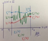
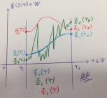
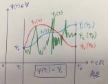
hence a different “histories” $\varphi\left(\psi,t,X_{\mathrm{env}}\left(\gamma\left(t\right)\right)\right)$ of the dynamics of the system. Since the noises $\gamma$ may describe any continuous trajectory for $t\in\left[t_{\mathrm{i}},t_{\mathrm{f}}\right]$, as illustrated in the cartoon of Figure 1, also the corresponding dynamics $\varphi\left(\psi,t,X_{\mathrm{env}}\left(\gamma\left(t\right)\right)\right)$ will have any continuous shape as a curve in $\mathbb{W}$, see Figure 2. This explains in a pictorial way the fail of uniqueness of the solution to the stochastic Cauchy problem (10): the randomness transits from noises $\gamma$ to dynamics $\varphi$, and from dynamics to the solution of the Cauchy problem $\psi\left(t\right)$, see Figure 3 for the final step of the pictorial explanation. Note that, even if all of the three solutions to (10) start at the same initial value, they develop very differently and the uniqueness invoked by DP is lost.

The random nature of each term $\gamma\left(t\right)$ in (9) and (10) renders it useful to consider the sample space $\Sigma\left(t_{\mathrm{i}},t_{\mathrm{f}}\right)$ of all the possible continuous trajectories $\gamma\left(t\right)$ in $\Xi$ with $t\in\left[t_{\mathrm{i}},t_{\mathrm{f}}\right]$, i.e. the sample space of all the possible realizations of the stochastic process $\gamma:\mathbb{R}\mapsto\Xi$. The set $\Sigma\left(t_{\mathrm{i}},t_{\mathrm{f}}\right)$ is infinite dimensional, namely $\Sigma\left(t_{\mathrm{i}},t_{\mathrm{f}}\right)\subseteq\mathcal{C}\left(\mathbb{R},\Xi\right)$; a probability measure defined on it, should be possibly based upon the functional counterpart of what an ordinary probability distribution function is for finite dimensional sample spaces, $\mathcal{P}\left[\gamma;t_{\mathrm{i}},t_{\mathrm{f}}\right)$. In this script

$$\mathcal{P}\left[\gamma;t_{\mathrm{i}},t_{\mathrm{f}}\right),$$

the square bracket left to $\gamma$ means that $\mathcal{P}$ depends on the infinite number of values $\gamma\left(t\right)$ (one per each $t\in\left[t_{\mathrm{i}},t_{\mathrm{f}}\right]$), while the round bracket right after $t_{\mathrm{f}}$ indicates that $\mathcal{P}$ depends also on the two real variables $t_{\mathrm{i}}$ and $t_{\mathrm{f}}$. The $\mathcal{P}\left[\gamma;t_{\mathrm{i}},t_{\mathrm{f}}\right)$ is referred to as realization probability functional (RPF) of $\gamma$, and its normalization condition reads:

$$\int_{\Sigma\left(t_{\mathrm{i}},t_{\mathrm{f}}\right)}\mathcal{P}\left[\gamma;t_{\mathrm{i}},t_{\mathrm{f}}\right)\left[d\gamma\right]=1.$$ (11)

In this (11) the symbol $\left[d\gamma\right]$ indicates the functional integral on $\Sigma\left(t_{\mathrm{i}},t_{\mathrm{f}}\right)$ of the stochastic terms, namely the continuous product:

$$\int_{\Sigma\left(t_{\mathrm{i}},t_{\mathrm{f}}\right)}\left[d\gamma\right]...=\prod_{t\in\left[t_{\mathrm{i}},t_{\mathrm{f}}\right]}\int_{\Xi}d\gamma\left(t\right)...$$

(see [4] for a thorough explanation of this). About the RPF $\mathcal{P}\left[\gamma;t_{\mathrm{i}},t_{\mathrm{f}}\right)$, it must be stressed that this will be expressable as the continuous product of all the $P_{t}\left(\gamma\right)^{dt}$ (see (9) and (10)), for $t\in\left[t_{\mathrm{i}},t_{\mathrm{f}}\right]$, only for time-$\delta$-correlated noises, see § 2.2: assigning the functional $\mathcal{P}\left[\gamma;t_{\mathrm{i}},t_{\mathrm{f}}\right)$ is then more powerful than giving all the time-local PDFs $P_{t}\left(\gamma\right)$, because $\mathcal{P}\left[\gamma;t_{\mathrm{i}},t_{\mathrm{f}}\right)$ contains any type of correlation among noises, that the collection of the PDFs does not, and indeed the latter is equivalent to the RPF only for the $\delta$-correlated stochastic variables. In fully mathematical terms, one could write:

$$P_{t}\left(\gamma\right)=\int_{t^{\prime}\neq t}\left[d\gamma\left(t^{\prime}\right)\right]\mathcal{P}\left[\gamma;t_{\mathrm{i}},t_{\mathrm{f}}\right)\ \forall\ t\in\left[t_{\mathrm{i}},t_{\mathrm{f}}\right].$$

Figure 1: Three possible realizations of the noise $\gamma\left(t\right)$ between $t_{\mathrm{i}}$ and $t_{\mathrm{f}}$: as $\gamma\left(t\right)$ can be any possible continuous curve in $\Xi$, here we have drawn two rather regular curves $\gamma_{1}\left(t\right)$ and $\gamma_{3}\left(t\right)$, and a less regular, sharp-cornered one $\gamma_{2}\left(t\right)$.

Figure 2: The cartoon of the three realizations of the process $\varphi\left(\psi,t,X_{\mathrm{env}}\left(\gamma\left(t\right)\right)\right)$ corresponding to the realizations $\gamma_{1}\left(t\right)$, $\gamma_{2}\left(t\right)$ and $\gamma_{3}\left(t\right)$ cited in Figure 1.

Figure 3: The cartoon of the three solutions $\psi_{i=1,2,3}\left(t\right)$ of a stochastic Cauchy problem as (10) corresponding to the realizations $\gamma_{1}\left(t\right)$, $\gamma_{2}\left(t\right)$ and $\gamma_{3}\left(t\right)$ in Figure 1.

In what follows, the program is to start with some particular form of the SDE in (10), in which one will understand how to pass from the ensemble statistics of noises $\gamma\left(t\right)$ to that of the system realizations $\psi\left(t\right)$, considering the interplay between the deterministic and the stochastic features of $\varphi$:

$$\mathcal{P}\left[\gamma;t_{\mathrm{i}},t_{\mathrm{f}}\right)\overset{\varphi}{\mapsto}\mathcal{A}\left[\psi;t_{\mathrm{i}},t_{\mathrm{f}}\right),$$ (12)

where $\mathcal{A}\left[\psi;t_{\mathrm{i}},t_{\mathrm{f}}\right)$ is the RPF of the stochastic process $\psi:\left[t_{\mathrm{i}},t_{\mathrm{f}}\right]\mapsto\mathbb{V}$, while the script $\overset{\varphi}{\mapsto}$ means that this pass is done thanks to the form of $\varphi$.

For the types of SDE we are going to work with, the scheme to perform the transition (12) includes the introduction of the concept of stochastic Lagrangian (SL), that will be introduced in § 2. Then, in § 3 the machinery will be applied to some particular case of physical relevance.

2 Functional Formalism for Statistical Dynamics

The mathematical quantity $\psi$, that describes the state of the system, is in general given by a certain number of components, indicated as $\psi^{I}$, so locally $\mathbb{V}$ will be described as some $\mathbb{R}^{n}$ (or $\mathbb{C}^{n}$) space, as $I=1,...,n$. Remarkably, an infinite dimensional state may well be necessary, e.g. in a classical continuum theory, in which the system is described by the local properties of the continuum, so that the index $I$ of $\psi$ will rather be some continuous position $\vec{x}$ in the three dimensional space. The functional formalism is described here for a general finite dimensional system, while in [5, 6, 7, 8] an infinite dimensional system, namely magneto-hydrodynamics, is considered.

Let’s go back to the SDE in (10), and consider a particular class of functions $\varphi\left(\psi,t,X_{\mathrm{env}}\left(\gamma\left(t\right)\right)\right)$ of the noises $\gamma$. Let us assume that the noises enter the dynamical equation (DE) of $\psi$ both in an additive form, as (8), and in a multiplicative way. In particular, as we assume the phase space $\mathbb{V}$ to be $n$-dimensional, let us consider two stochastic $n$-vectors, one of components $f^{I}$ and the other of components $g_{J}$, whose statistics is assigned through their RPF $\mathcal{P}\left[f,g;t_{\mathrm{i}},t_{\mathrm{f}}\right)$, and appearing in the SDE of $\psi$ as:

$$\dfrac{d\psi^{I}}{dt}=\Lambda\left(\psi\right)+g_{J}\left(t\right)\Gamma^{JI}\left(\psi\right)+f^{I}\left(t\right).$$ (13)

In (13) one has the co-existence of deterministic expressions, depending on $\psi$

$$\Lambda\in\mathcal{C}^{\infty}\left(\mathbb{V},\mathrm{T}\left(\mathbb{V}\right)\right),\ \Gamma\in\mathcal{C}^{\infty}\left(\mathbb{V},\mathrm{T}\left(\mathbb{V}\right)\otimes\mathrm{T}\left(\mathbb{V}\right)\right),$$

with that of the noise terms $f$ and $g$, of which one supposes to know the statistics via $\mathcal{P}\left[f,g;t_{\mathrm{i}},t_{\mathrm{f}}\right)$.

Equation (13) might appear rather particular and simple, as a form of SDE: it is clearly more complicated than the simplest case (8), but one may well think more involuted expressions, as for instance

$$\dfrac{d\psi}{dt}=\Lambda\left(\psi\right)+G\exp\left(\frac{A\psi^{2}+\gamma\left(t\right)}{B\cos\left(\gamma\left(t\right)\right)}\right)...,$$

being $\mathbb{V}=\mathbb{R}$ for simplicity. The point is that:

• the “simple” form (13) is the one allowing for the formalism of stochastic Lagrangian, that is of interest here;

• however, as well explained in [5, 6, 7, 8], and in [9], important realistic systems as space plasmas may be described by (13).

Our work will then concentrate on the stochastic Cauchy problem:

$$\begin{cases}&\dfrac{d\psi^{I}}{dt}=\Lambda\left(\psi\right)+g_{J}\left(t\right)\Gamma^{JI}\left(\psi\right)+f^{I}\left(t\right),\\ \\ &\psi\left(t_{\mathrm{i}}\right)=\psi_{\mathrm{i}},\\ \\ &\left(f\left(t\right),g\left(t\right)\right)\sim\mathcal{P}\left[f,g;t_{\mathrm{i}},t_{\mathrm{f}}\right):\thinspace\Sigma\left(t_{\mathrm{i}},t_{\mathrm{f}}\right)\mapsto\mathbb{R}^{+}.\end{cases}$$ (14)

As the paper [10] by Phythian is the first paper introducing this formalism, we will refer to (13) as Langevin-Phythian Equation (LPE) (as far as the Author is aware of, the formalism of the stochastic Lagrangian has been introduced in [10] and in [11]).

Before going ahead, notice that in the SDE (13), and in the system (14), noises seem to appear “directly” without the mediation of the environmental variables $X_{\mathrm{env}}$ in (10): this is only an appearance, as the reader may get convinced of going through [5]. In that case, e.g., noise terms are identified with the terms $-\vec{\partial}\times\left(\zeta\cdot\vec{J}\right)$, $\frac{\vec{J}}{\rho}$ and $-\frac{\vec{\partial}p}{\rho}$, being $\zeta$ the plasma conductivity tensor, $\vec{J}$ the electric current, $\rho$ the plasma mass density and $p$ the plasma pressure: as the state of the system $\psi=\left(\vec{V},\vec{B}\right)$ included, there, the plasma bulk velocity and the magnetic induction vector, the quantities $\zeta$, $\vec{J}$, $\rho$ and $p$ could be understood as “environmental variables” forcing $\psi$. Following this suggestion, one forms noises with quantities determined by the microscopic nature of the continuum, the microscopic stochastically treated degrees of freedom (μSTDoF, see also [12] for this concept) of which are the “environment” for the otherwise isolated fluid variable system.

The dynamics governed by conditions (14) will produce a multi-history evolution for $\psi$: as pictorially indicated in Figure 3, the system history between $t_{\mathrm{i}}$ and $t_{\mathrm{f}}$ is “statistically distributed” along many elements of $\Sigma\left(t_{\mathrm{i}},t_{\mathrm{f}}\right)$, according to the RPF $\mathcal{A}\left[\psi;t_{\mathrm{i}},t_{\mathrm{f}}\right)$ that will depend on the noise RPF $\mathcal{P}\left[f,g;t_{\mathrm{i}},t_{\mathrm{f}}\right)$ via

$$\mathcal{P}\left[f,g;t_{\mathrm{i}},t_{\mathrm{f}}\right)\overset{\Lambda,\Gamma}{\mapsto}\mathcal{A}\left[\psi;t_{\mathrm{i}},t_{\mathrm{f}}\right),$$ (15)

that is the version of (12) adapted to the dynamics (14). The theoretical program we want to pursue here is to calculate the map just mimicked in (15), i.e. to obtain a (closed as possible) expression of the RPF of $\psi$ from that of the RPF of the noises $f$ and $g$, and the deterministic parts $\Lambda$ and $\Gamma$ of (14) (precisely, the competition between chance and necessity about which Haken speaks in his book [13] about “Synergetics”).

Once the RPF $\mathcal{A}\left[\psi;t_{\mathrm{i}},t_{\mathrm{f}}\right)$ is given, the following program may be realized:

1. evaluate any statistical quantity $\left\langle F\right\rangle$, for any functional $F\left[\psi\right]$, on the ensemble $\Sigma\left(t_{\mathrm{i}},t_{\mathrm{f}}\right)$ of trajectories through $\mathbb{V}$ admitted for the dynamics (14);

2. calculate the transition probability $\mathcal{P}_{\psi_{\mathrm{i}}\mapsto\psi_{\mathrm{f}}}\left(t_{\mathrm{i}},t_{\mathrm{f}}\right)$ for the system from an initial condition $\psi_{\mathrm{i}}=\psi\left(t_{\mathrm{i}}\right)$ and a final one $\psi_{\mathrm{f}}=\psi\left(t_{\mathrm{f}}\right)$.

Both any $\left\langle F\right\rangle$ and the transition probability $\mathcal{P}_{\psi_{\mathrm{i}}\mapsto\psi_{\mathrm{f}}}\left(t_{\mathrm{i}},t_{\mathrm{f}}\right)$ may be expressed in terms of $\mathcal{A}\left[\psi;t_{\mathrm{i}},t_{\mathrm{f}}\right)$. The quantity $\left\langle F\right\rangle$ in Point 1 is calculated as

$$\left\langle F\right\rangle=\int_{C\left(\left[t_{\mathrm{i}},t_{\mathrm{f}}\right],\mathbb{V}\right)}\left[d\psi\right]F\left[\psi\right]\mathcal{A}\left[\psi;t_{\mathrm{i}},t_{\mathrm{f}}\right),$$ (16)

where it is intended that $F\left[\psi\right]$ depends on the whole trajectory $\psi\left(t\right)$ for $t\in\left[t_{\mathrm{i}},t_{\mathrm{f}}\right]$: actually, the prescription (16) may work also for a time-local function $F\left(\psi\right)$, that can always be expressed as an integration with the presence of some $\delta\left(t-\hat{t}\right)$, provided $\hat{t}$ is the instant of interest to calculate the function.

The transition probability $\mathcal{P}_{\psi_{\mathrm{i}}\mapsto\psi_{\mathrm{f}}}\left(t_{\mathrm{i}},t_{\mathrm{f}}\right)$ may be calculated as the integration of $\mathcal{A}\left[\psi;t_{\mathrm{i}},t_{\mathrm{f}}\right)$ on all the possible configurations $\psi\left(t\right)\thinspace/\thinspace t\in\left(t_{\mathrm{i}},t_{\mathrm{f}}\right)$, while the initial and final configurations $\psi\left(t_{\mathrm{i}}\right)$ and $\psi\left(t_{\mathrm{f}}\right)$ are not integrated on, and kept fixed to the values of interest $\psi_{\mathrm{i}}$ and $\psi_{\mathrm{f}}$ respectively. One may write

$$\mathcal{P}_{\psi_{\mathrm{i}}\mapsto\psi_{\mathrm{f}}}\left(t_{\mathrm{i}},t_{\mathrm{f}}\right)=\lim_{\epsilon\rightarrow 0}\int_{C\left(\left[t_{\mathrm{i}}+\epsilon,t_{\mathrm{f}}-\epsilon\right],\mathbb{V}\right)}\left[d\psi\right]\left.\mathcal{A}\left[\psi;t_{\mathrm{i}},t_{\mathrm{f}}\right)\right|_{\psi\left(t_{\mathrm{i}}\right)=\psi_{\mathrm{i}},\thinspace\psi\left(t_{\mathrm{f}}\right)=\psi_{\mathrm{f}}}.$$ (17)

This may be also written as

$$\mathcal{P}_{\psi_{\mathrm{i}}\mapsto\psi_{\mathrm{f}}}\left(t_{\mathrm{i}},t_{\mathrm{f}}\right)=\left.\left\langle 1\right\rangle\right|_{\psi\left(t_{\mathrm{i}}\right)=\psi_{\mathrm{i}},\thinspace\psi\left(t_{\mathrm{f}}\right)=\psi_{\mathrm{f}}}.$$ (18)

2.1 Stochastic Lagrangian

The program stated in Points 1 and 2 before needs the knowledge of $\mathcal{A}\left[\psi;t_{\mathrm{i}},t_{\mathrm{f}}\right)$: in this work the RPF of $\psi$ is represented through a time-local function $\mathcal{\mkern 2.0mu\mathchar 32\relax\mkern-7.0muL}\left(\frac{d\psi}{dt},\psi\right)$, so that

$$\begin{cases}&\mathcal{A}\left[\psi;t_{\mathrm{i}},t_{\mathrm{f}}\right)=N_{0}\left(t_{\mathrm{i}},t_{\mathrm{f}}\right)\exp\left[-i\int_{t_{\mathrm{i}}}^{t_{\mathrm{f}}}\mathcal{\mkern 2.0mu\mathchar 32\relax\mkern-7.0muL}\left(\frac{d\psi}{dt}\left(t\right),\psi\left(t\right)\right)dt\right],\\ \\ &\dfrac{1}{N_{0}\left(t_{\mathrm{i}},t_{\mathrm{f}}\right)}\overset{\mathrm{def}}{=}\int_{C\left(\left[t_{\mathrm{i}},t_{\mathrm{f}}\right],\mathbb{V}\right)}\left[d\psi\right]e^{-i\int_{t_{\mathrm{i}}}^{t_{\mathrm{f}}}\mathcal{\mkern 2.0mu\mathchar 32\relax\mkern-7.0muL}\left(\frac{d\psi}{dt}\left(t\right),\psi\left(t\right)\right)dt}.\end{cases}$$ (19)

Clearly, the term $N_{0}\left(t_{\mathrm{i}},t_{\mathrm{f}}\right)$ is a normalization factor, so that the condition

$$\int_{C\left(\left[t_{\mathrm{i}},t_{\mathrm{f}}\right],\mathbb{V}\right)}\left[d\psi\right]\mathcal{A}\left[\psi;t_{\mathrm{i}},t_{\mathrm{f}}\right)=1$$ (20)

holds. The time-local function $\mathcal{\mkern 2.0mu\mathchar 32\relax\mkern-7.0muL}\left(\frac{d\psi}{dt},\psi\right)$ is referred to as stochastic Lagrangian (SL).

Since the relationship between this $\mkern 2.0mu\mathcal{\mkern 2.0mu\mathchar 32\relax\mkern-7.0muL}\left(\frac{d\psi}{dt},\psi\right)$ and the RPF $\mathcal{A}$ of the stochastic process is the same that one has between the classical Lagrangian function and the quantum amplitude in Quantum Mechanics [14], also here one may expect the “symmetries” of $\mathcal{\mkern 2.0mu\mathchar 32\relax\mkern-7.0muL}$ to turn into invariances of the system statistics. One has to add that, for real $\psi$, as transition probabilities $\mathcal{P}_{\psi_{\mathrm{i}}\mapsto\psi_{\mathrm{f}}}\left(t_{\mathrm{i}},t_{\mathrm{f}}\right)$ must be real positive numbers, the quantity $\mathcal{\mkern 2.0mu\mathchar 32\relax\mkern-7.0muL}\left(\frac{d\psi}{dt},\psi\right)$ must be an imaginary number, as it happens indeed in real cases [5, 7].

About the stochastic Lagrangian $\mathcal{\mkern 2.0mu\mathchar 32\relax\mkern-7.0muL}\left(\frac{d\psi}{dt},\psi\right)$ one has to stress that it is a function intrinsically different from what one calls “Lagrangian” in Analytical Mechanics: indeed, this Lagrangian $\mathcal{\mkern 2.0mu\mathchar 32\relax\mkern-7.0muL}\left(\frac{d\psi}{dt},\psi\right)$, contains the maximum time-derivative appearing in the ODE of the system (13), that is an intrinsically first order ODE, while the Lagrangian of Analytical Mechanics $L\left(\frac{d\underline{q}}{dt},\underline{q}\right)$ does not contain the maximum order time-derivative of the evolution equation of the system, as Euler-Lagrange equations $\frac{d}{dt}\left(\frac{\partial L}{\partial\underline{\dot{q}}}\right)-\frac{\partial L}{\partial\underline{q}}=0$ are second order ODEs (here the dot means time-derivative, as $\dot{\underline{q}}\overset{\mathrm{def}}{=}\frac{d\underline{q}}{dt}$ and $\dot{\psi}\overset{\mathrm{def}}{=}\frac{d\psi}{dt}$). In § 3.1, where the case of a point particle undergoing classical and stochastic forces is treated, the difference between $\mathcal{\mkern 2.0mu\mathchar 32\relax\mkern-7.0muL}$ and the would-be-Lagrangian $L$ of the point prticle without noise is apparent: indeed, where the traditional Lagrangian would be $L\left(\dot{\vec{x}},\vec{x}\right)$, a function of position and velocity, the stochastic Lagrangian is some more complicated function $\mathcal{\mkern 2.0mu\mathchar 32\relax\mkern-7.0muL}\left(\dot{\vec{x}},\dot{\vec{p}},\vec{x},\vec{p}\right)$, depending on position, velocity, momentum and momentum derivative. Last difference we need to stress between the Analytical Mechanics Lagrangian $L$ and the stochastic Lagrangian $\mathcal{\mkern 2.0mu\mathchar 32\relax\mkern-7.0muL}$ is that, while $L$ contains “all the Physics” of the system only for conservative systems, $\mathcal{\mkern 2.0mu\mathchar 32\relax\mkern-7.0muL}$ encodes the whole Physics of any stochastic system in the form (13), regardless it is conservative (Hamiltonian, see § 3.2.1), or dissipative (metriplectic, see § 3.2.2).

It is also of use to give the definition of stochastic action $\mathcal{\mathchoice{\underaccent{\displaystyle\mathchar 24\relax}{S}}{\underaccent{\textstyle\mathchar 24\relax}{S}}{\underaccent{\scriptstyle\mathchar 24\relax}{S}}{\underaccent{\scriptscriptstyle\mathchar 24\relax}{S}}}\left[\psi,t_{\mathrm{i}},t_{\mathrm{f}}\right)$ as the time-integral of the Lagrangian $\mathcal{\mkern 2.0mu\mathchar 32\relax\mkern-7.0muL}$:

$$\mathcal{\mathchoice{\underaccent{\displaystyle\mathchar 24\relax}{S}}{\underaccent{\textstyle\mathchar 24\relax}{S}}{\underaccent{\scriptstyle\mathchar 24\relax}{S}}{\underaccent{\scriptscriptstyle\mathchar 24\relax}{S}}}\left[\psi,t_{\mathrm{i}},t_{\mathrm{f}}\right)\overset{\mathrm{def}}{=}\int_{t_{\mathrm{i}}}^{t_{\mathrm{f}}}dt\mathcal{\mkern 2.0mu\mathchar 32\relax\mkern-7.0muL}\left(\frac{d\psi}{dt},\psi\right),$$ (21)

so that $\mathcal{A}=N_{0}\exp\left(-i\mathcal{\mathchoice{\underaccent{\displaystyle\mathchar 24\relax}{S}}{\underaccent{\textstyle\mathchar 24\relax}{S}}{\underaccent{\scriptstyle\mathchar 24\relax}{S}}{\underaccent{\scriptscriptstyle\mathchar 24\relax}{S}}}\right)$. The caveat to make no confusion between this $\mathcal{\mathchoice{\underaccent{\displaystyle\mathchar 24\relax}{S}}{\underaccent{\textstyle\mathchar 24\relax}{S}}{\underaccent{\scriptstyle\mathchar 24\relax}{S}}{\underaccent{\scriptscriptstyle\mathchar 24\relax}{S}}}$ and the action of Analytical Mechanics is the same one as that of not confusing the stochastic $\mathcal{\mkern 2.0mu\mathchar 32\relax\mkern-7.0muL}$ and the mechanical Lagrangian $L$ discussed just now.

The construction of the SL is described in [10], and inspired by the previous literature cited therein. In particular, thanks to the mathematical nature of the LPE (13), it is possible to introduce the kernel $\mathcal{A}\left[\psi;t_{\mathrm{i}},t_{\mathrm{f}}\right)$ starting from the definition of an ensemble statistical average $\left\langle F\right\rangle$, based on noise statistics

$$\left\langle F\right\rangle\overset{\mathrm{def}}{=}\left\langle F\right\rangle_{f,g},$$

as noises represent the only element giving to (14) a stochastic character. The definition of the average $\left\langle F\right\rangle_{f,g}$ is obviously

$$\left\langle F\right\rangle_{f,g}\overset{\mathrm{def}}{=}\int_{\Sigma\left(t_{\mathrm{i}},t_{\mathrm{f}}\right)}F\left[\psi\right]\mathcal{P}\left[f,g;t_{\mathrm{i}},t_{\mathrm{f}}\right)\left[df\right]\left[dg\right]:$$

our program is to obtain an expression of $\mathcal{A}$ so that

$$\int_{\Sigma\left(t_{\mathrm{i}},t_{\mathrm{f}}\right)}\left[df\right]\int_{\Sigma\left(t_{\mathrm{i}},t_{\mathrm{f}}\right)}\left[dg\right]F\left[\psi\right]\mathcal{P}\left[f,g;t_{\mathrm{i}},t_{\mathrm{f}}\right)=\int_{C\left(\left[t_{\mathrm{i}},t_{\mathrm{f}}\right],\mathbb{V}\right)}\left[d\psi\right]F\left[\psi\right]\mathcal{A}\left[\psi;t_{\mathrm{i}},t_{\mathrm{f}}\right)\ \forall\thinspace F.$$ (22)

The first step taken in [10] to obtain $\mathcal{A}$ satisfying (22), is to consider $n$ auxiliary variables $\chi_{I=1,...,n}$ that in a sense represent the Fourier momenta conjugated with the additive noises $f^{I=1,...,n}$ in the functional space $\Sigma\left(t_{\mathrm{i}},t_{\mathrm{f}}\right)$. Then, an auxiliary kernel, depending on $\psi$ and $\chi$ is defined as:

$$\begin{cases}&A\left[\psi,\chi;t_{\mathrm{i}},t_{\mathrm{f}}\right)=\\ \\ &=A_{0}\left(t_{\mathrm{i}},t_{\mathrm{f}}\right)C\left[\chi,\Gamma;t_{\mathrm{i}},t_{\mathrm{f}}\right)e^{-i\int_{t_{\mathrm{i}}}^{t_{\mathrm{f}}}dt\left[\dot{\psi}^{I}\chi_{I}-\Lambda^{I}\left(\psi\right)\chi_{I}-\frac{i}{2}\frac{\partial}{\partial\psi^{I}}\Lambda^{I}\left(\psi\right)\right]},\\ \\ \\ &C\left[\chi,\Gamma;t_{\mathrm{i}},t_{\mathrm{f}}\right)=\\ \\ &=\left\langle e^{i\int_{t_{\mathrm{i}}}^{t_{\mathrm{f}}}dt\left[f^{I}\chi_{I}+g_{I}\Gamma^{IJ}\left(\psi\right)\chi_{J}+g_{I}\frac{\partial}{\partial\psi^{J}}\Gamma^{IJ}\left(\psi\right)\right]}\right\rangle_{f,g}.\end{cases}$$ (23)

In (23) the quantity $A_{0}\left(t_{\mathrm{i}},t_{\mathrm{f}}\right)$ is a normalization factor, so that

$$\int_{C\left(\left[t_{\mathrm{i}},t_{\mathrm{f}}\right],\mathrm{T}\left(\mathbb{V}^{*}\right)\right)}\left[d\chi\right]\int_{C\left(\left[t_{\mathrm{i}},t_{\mathrm{f}}\right],\mathbb{V}\right)}\left[d\psi\right]A\left[\psi,\chi;t_{\mathrm{i}},t_{\mathrm{f}}\right)=1;$$

the factor $C\left[\chi,\Gamma;t_{\mathrm{i}},t_{\mathrm{f}}\right)$ is the term in which the noise statistics ends up being encoded, as

$$C\left[\chi,\Gamma;t_{\mathrm{i}},t_{\mathrm{f}}\right)=\int_{\Sigma\left(t_{\mathrm{i}},t_{\mathrm{f}}\right)}\left[df\right]\int_{\Sigma\left(t_{\mathrm{i}},t_{\mathrm{f}}\right)}\left[dg\right]e^{i\int_{t_{\mathrm{i}}}^{t_{\mathrm{f}}}dt\left[f^{I}\chi_{I}+g_{I}\Gamma^{IJ}\left(\psi\right)\chi_{J}+g_{I}\frac{\partial}{\partial\psi^{J}}\Gamma^{IJ}\left(\psi\right)\right]}\mathcal{P}\left[f,g;t_{\mathrm{i}},t_{\mathrm{f}}\right).$$

Once the auxiliary kernel $A\left[\psi,\chi;t_{\mathrm{i}},t_{\mathrm{f}}\right)$ is constructed, the definition of the physical kernel $\mathcal{A}\left[\psi;t_{\mathrm{i}},t_{\mathrm{f}}\right)$ reads simply:

$$\mathcal{A}\left[\psi;t_{\mathrm{i}},t_{\mathrm{f}}\right)\overset{\mathrm{def}}{=}\int_{C\left(\left[t_{\mathrm{i}},t_{\mathrm{f}}\right],\mathrm{T}\left(\mathbb{V}^{*}\right)\right)}\left[d\chi\right]A\left[\psi,\chi;t_{\mathrm{i}},t_{\mathrm{f}}\right).$$ (24)

The calculation indicated in (24) is nothing but obvious, its feasibility is definitely not for grant. Indeed, summing over all the possible histories $\chi\left(t\right)\thinspace/\thinspace t\in\left[t_{\mathrm{i}},t_{\mathrm{f}}\right]$ is still matter of being able to do a functional integration, that we know is not an easy task in general. In § 2.2 we will see this integration is rather tractable if noises $f$ and $g$ are Gaussian fluctuations $\delta$-correlated in time, as in (25).

The great effort is then re-casting the RPF defined as (24) and (23) in the Lagrangian form (19).

2.2 $\delta$-correlated Gaussian noise

The example in which the calculations indicated in (23) and (24) are completely, and rather easily, feasible, is that in which $f\left(t\right)$ and $g\left(t\right)$ are time-$\delta$-correlated noises with $t$-local Gaussian PDF. Let us assume that the two noises $f$ and $g$ have $t$-local probability density functions

$$\begin{cases}&P_{t}\left(f\right)=\sqrt{\frac{2^{n-1}\left\|\lambda\left(t\right)\right\|}{\pi}}e^{-\lambda_{IJ}\left(t\right)\left(f^{I}-f_{0}^{I}\right)\left(f^{J}-f_{0}^{J}\right)},\\ \\ &Q_{t}\left(g\right)=\sqrt{\frac{2^{n-1}\left\|\mu\left(t\right)\right\|}{\pi}}e^{-\mu_{IJ}\left(t\right)\left(g^{I}-g_{0}^{I}\right)\left(g^{J}-g_{0}^{J}\right)}.\end{cases}$$ (25)

As noises taken at different times are independent of each other, the whole RPF is a continuous product of the time-local PDFs, i.e.:

$$\begin{array}[]{c}\mathcal{P}\left[f,g;t_{\mathrm{i}},t_{\mathrm{f}}\right)={\displaystyle\prod_{t\in\left[t_{\mathrm{i}},t_{\mathrm{f}}\right]}}\left(\frac{2^{2\left(n-1\right)}\left\|\lambda\left(t\right)\right\|\left\|\mu\left(t\right)\right\|}{\pi^{2}}\right)^{\frac{dt}{2}}*\\ \\ e^{-\int_{t_{\mathrm{i}}}^{t_{\mathrm{f}}}dt\left[\lambda_{IJ}\left(t\right)\left(f^{I}\left(t\right)-f_{0}^{I}\left(t\right)\right)\left(f^{J}\left(t\right)-f_{0}^{J}\left(t\right)\right)+\mu_{IJ}\left(t\right)\left(g^{I}\left(t\right)-g_{0}^{I}\left(t\right)\right)\left(g^{J}\left(t\right)-g_{0}^{J}\left(t\right)\right)\right]}\end{array}$$ (29)

(in the expression (29) the emergence of the integration $\int_{t_{\mathrm{i}}}^{t_{\mathrm{f}}}dt...$ in the argument of the exponential, as well as the power $\frac{dt}{2}$ in the normalization factor, come from the continuous product, see [4]). About the coefficients $\lambda$ and $\mu$ in (25) and (29), one has to note that their relationship with the standard deviation $\sigma_{f}$ and $\sigma_{g}$ of noises reads:

$$\lambda=\frac{1}{2\sigma_{f}^{2}},\ \mu=\frac{1}{2\sigma_{g}^{2}}$$ (30)

(all the quantities in (30) are $\mathbb{R}^{n,n}$ matrices). A further assumption necessary for (29) to represent the correct RPF of those noises, is that $f$ and $g$ are uncorrelated with each other, i.e.:

$$\left\langle f^{I}\left(t\right)g^{J}\left(t^{\prime}\right)\right\rangle=0\ \forall\thinspace t,t^{\prime},I,J.$$

The RPF (29) gives rise to the average over noises:

$$\left\langle F\right\rangle_{f,g} =\left(\prod_{t\in\left[t_{\mathrm{i}},t_{\mathrm{f}}\right]}\left(\frac{2^{2\left(n-1\right)}\left\|\lambda\left(t\right)\right\|\left\|\mu\left(t\right)\right\|}{\pi^{2}}\right)^{\frac{dt}{2}}\int_{\mathbb{R}^{n}}df\left(t\right)\int_{\mathbb{R}^{n}}dg\left(t\right)\right)*$$

$$*F\left[\psi\right]e^{-\int_{t_{\mathrm{i}}}^{t_{\mathrm{f}}}dt\left[\lambda_{IJ}\left(t\right)\left(f^{I}\left(t\right)-f_{0}^{I}\left(t\right)\right)\left(f^{J}\left(t\right)-f_{0}^{J}\left(t\right)\right)+\mu_{IJ}\left(t\right)\left(g^{I}\left(t\right)-g_{0}^{I}\left(t\right)\right)\left(g^{J}\left(t\right)-g_{0}^{J}\left(t\right)\right)\right]}.$$

Without loss of generality one may put

$${\lambda }_{IJ}={\lambda }^{\left(I\right)}{\delta }_{IJ},{\mu }_{IJ}={\mu }^{\left(I\right)}{\delta }_{IJ},$$

References

- [1] Newton, I. Philosophiae Naturalis Principia Mathematica - Editio Tertia. G. & J. Innys, Royal Society, 1726.
- [2] Materassi, M., Collini, D., Barletti, L. Pack behaviour in inter-algal competition, in preparation.
- [3] Dirac P.A.M. The Principles of Quantum Mechanics. 3rd Edition, Oxford University Press, Amen House, London E.C.4 (1947).
- [4] Materassi, M. Stochastic Field Theory for the Ionospheric Fluctuations in Equatorial Spread F, Chaos, Solitons and Fractals 121 (2019) 186–210.
- [5] Materassi, M., Consolini, G., Turning the resistive MHD into a stochastic field theory, (2008) Nonlinear Processes in Geophysics, 15 (4), pp. 701-709.
- [6] Materassi, M., Stochastic Lagrangian for the 2D Visco-Resistive Magneto-Hydrodynamics, Plasma Phys. Control. Fusion 52 (2010) 075004.
- [7] Materassi M., G. Consolini, The Stochastic Tetrad MHD via Functional Formalism, J. Plasma Phys.(2015), vol. 81, 495810602, Cambridge University Press 2015, doi:10.1017/S0022377815001105.
- [8] Quattrociocchi, V., Consolini, G., Marcucci, M. F., Materassi, M., On Geometrical Invariants of Magnetic Field Gradient Tensor in Turbulent Space Plasmas: Scale Variability in the Inertial Range, The Astrophysical Journal, 878 (2), 2019.
- [9] Chang, T. Self-organized criticality, multi-fractal spectra, sporadic localized reconnections and intermittent turbulence in the magnetotail. Physics of Plasmas 6, 4137 (1999); https://doi.org/10.1063/1.873678.
- [10] Phythian, R., The functional formalism of classical statistical dynamics, Journal of Physics A: Mathematical and General, Volume 10, Number 5.
- [11] Jouvet, B., Phythian, R. Quantum aspects of classical and statistical fields. Physical Review A, 19 (3), 1979.
- [12] Materassi M., Entropy as a Metric Generator of Dissipation in Complete Metriplectic Systems, Special issue Selected Papers from 2nd International Electronic Conference on Entropy and Its Applications of Entropy, Entropy 2016, 18, 304; doi:10.3390/e18080304.
- [13] Haken, H. Synergetics. An introduction. Springer-Verlag, Berlin-Heidelberg-New York-Tokyo, 1983.
- [14] Feynman, R. P., Hibbs, A. R. Quantum Mechanics and Path Integrals, McGraw Hill-International Series in the Earth and Planetary Sciences, McGraw-Hill College; First Edition edition (June 1, 1965).
- [15] Materassi, M., Granularity Meets Smoothness: Stochastic Approaches to (Space) Plasmas. Draft of theLectures for the Course “Complexity and Turbulence in Space Plasmas”, 18-22 September 2017, International School of Space Science, L’Aquila, Italy. Ask to the Author MM for a copy.
- [16] Guha, P. Metriplectic structure, Leibniz dynamics and dissipative systems. Journal of Mathematical Analysis and Applications 326 (1): 121-136.
- [17] Morrison, P.J. Hamiltonian Fluid Mechanics, in “Encyclopedia of Mathematical Physics”, vol. 2, (Elsevier, Amsterdam, 2006) p. 593.
- [18] Definition of “master equation” in Wikipedia - the free encyclopedia, see the webpage: https://en.wikipedia.org/wiki/Master_equation.