Low-memory, discrete ordinates, discontinuous Galerkin methods for radiative transport

Abstract

The discrete ordinates discontinuous Galerkin ($S_{N}$-DG) method is a well-established and practical approach for solving the radiative transport equation. In this paper, we study a low-memory variation of the upwind $S_{N}$-DG method. The proposed method uses a smaller finite element space that is constructed by coupling spatial unknowns across collocation angles, thereby yielding an approximation with fewer degrees of freedom than the standard method. Like the original $S_{N}$-DG method, the low memory variation still preserves the asymptotic diffusion limit and maintains the characteristic structure needed for mesh sweeping algorithms. While we observe second-order convergence in scattering dominated, diffusive regime, the low-memory method is in general only first-order accurate. To address this issue, we use upwind reconstruction to recover second-order accuracy. For both methods, numerical procedures based on upwind sweeps are proposed to reduce the system dimension in the underlying Krylov solver strategy.

65N35, 65N22, 65F50, 35J05

1 Introduction

Radiative transport equations [2, 9, 27, 25, 26, 12, 8] describe the flows of particles, such as photons, neutrons, and electrons, as they pass through and interact with a background medium. These equations are used in various applications, including astrophysics and nuclear reactor analysis.

In this paper, we consider the scaled, steady-state, linear transport equation

(1.1a) $$\Omega\cdot\nabla\Psi(\Omega,x)+\left(\frac{\sigma_{\mathrm{s}}(x)}{\varepsilon}+\varepsilon\sigma_{\mathrm{a}}(x)\right)\Psi(\Omega,x) =\frac{\sigma_{\mathrm{s}}(x)}{\varepsilon}\overline{\Psi}(x)+\varepsilon q(x), (\Omega,x)\in S\times D,$$

(1.1b) $$\Psi(\Omega,x) =\alpha(\Omega,x), (\Omega,x)\in\Gamma^{-}.$$

Here $D\subset\mathbb{R}^{d}$ $(d=1,2,3)$ is an open, bounded, and Lipschitz domain; $S$ is the projection of the unit sphere in $\mathbb{R}^{3}$ into $\mathbb{R}^{d}$ (the interval $[-1,1]$ for $d=1$ and unit disk for $d=2$); and $\Gamma^{-}=\{(x,\Omega)\in S\times\partial D\mid\Omega\cdot n(x)<0\}$, where $n(x)$ is the outward unit normal vector at any point $x\in\partial D$ where the boundary is $C^{1}$.

The angular flux $\Psi$ is the flux of particles at the location $x$ moving with unit speed in the direction $\Omega$, and the scalar flux $\overline{\Psi}=\frac{1}{|S|}\int_{S}\Psi d\Omega$ is the average of $\Psi$ over $S$. The functions $\sigma_{\mathrm{s}}$ and $\sigma_{\mathrm{a}}$ are (known) non-dimensionalized scattering and absorption cross-sections, respectively, and $q$ is a (known) non-dimensionalized source. The function $\alpha(\Omega,x)$ is the (known) incoming flux at $x\in\partial D$ moving in the direction $\Omega$. The constant $\varepsilon>0$ is a scaling parameter which characterizes the relative strength of scattering.

Designing effective numerical methods for (1.1) is a serious challenge, and the intent of this paper is to address two of the main issues. Firstly, for a three-dimensional problem, the unknown intensity $\Psi$ is a function of three spatial and two angular variables; the discretization of this five-dimensional phase space usually requires significant computational resources. Secondly, when the parameter $\varepsilon$ is small, $\Psi$ is nearly independent of $\Omega$ and can be approximated by the solution of a diffusion equation in the variable $x$ only [16, 5, 6]. That is, away from the boundary, $\Psi(\Omega,x)=\Psi^{(0)}(x)+O(\varepsilon)$ as $\varepsilon\to 0$, where $\Psi^{(0)}$ satisfies

(1.2) $$-\nabla\cdot\left(\frac{1}{3\sigma_{\mathrm{s}}}\nabla\Psi^{(0)}(x)\right)+\sigma_{\mathrm{a}}\Psi^{(0)}(x)=q(x),\quad x\in D,$$

along with appropriate boundary conditions. A numerical method for (1.1) should preserve this asymptotic limit without having to resolve the length scales associated with $\varepsilon$ [19]. In other words, in the limit $\varepsilon\to 0$, a discretization of the transport equation (1.1) should become a consistent and stable discretization of the diffusion equation (1.2). Otherwise a highly refined mesh is needed to approximate the solution accurately [22].

Classical approaches for discretizing (1.1) often involve separate treatment of the angular and spatial variables, and a variety of options are available. Among them, the $S_{N}$-DG method [17, 21, 1] has received significant attention due to it’s robustness, computational efficiency, and convenient implementation. The $S_{N}$ method (see[23] for a substantial review and additional references) is a collocation method in which the angular variable $\Omega$ is discretized into a finite number of directions and a quadrature rule is used to evaluate $\overline{\Psi}$. The $S_{N}$ discretization preserves non-negativity of $\Psi$ and can incorporate the boundary conditions from (1.1) in a straightforward way. It also preserves the characteristic structure of the advection operator in (1.1), which allows for the use of fast sweeping techniques for inverting the discrete form of the operator on the left-hand side of (1.1).

Discontinuous Galerkin (DG) methods are a class of finite element methods that construct numerical solutions using piecewise polynomial spaces. The DG approach was introduced in [29] for the express purpose of solving equations like (1.1), followed shortly thereafter by a rigorous analysis in [24]. Since then, DG methods have been applied to nonlinear hyperbolic conservation laws and convection-dominated problems [7], elliptic problems [3], and equations with higher-order derivatives [32, 31]. When used with upwind fluxes, DG methods preserve the characteristic structure of (1.1) that enables sweeps. Moreover, if the approximation space can support globally continuous linear polynomials, then DG methods with upwind fluxes will yield accurate numerical solutions for $\Psi$ without the need to resolve $\varepsilon$ with the spatial mesh [21, 1, 13]. However, this condition on the approximation space means that at least $P^{1}$ elements must be used for a triangular mesh and $Q^{1}$ elements for a rectangular mesh.

In order to reduce memory costs in the upwind $S_{N}$-DG method, while still preserving the asymptotic diffusion limit and maintaining the characteristic structure needed for sweeps, we propose in this paper to couple the finite element spaces between different collocation angles in the discrete ordinate approximation. Since the solution becomes isotropic in the diffusion limit ($\varepsilon\to 0$), we hypothesize that only a $P^{1}$ (for triangles) or $Q^{1}$ (for rectangles) approximation of the angular average is necessary. Thus, instead of using a tensor product finite element space for the $S_{N}$-DG system, we seek the solution in a proper subspace, in which all the elements have isotropic slopes. This choice of finite element space yields a significant reduction in memory per spatial cell, as illustrated in Table 1.1.

Unknowns per cell	Triangles ($P^{1}$)	Rectangles ($Q^{1}$)
Standard $S_{N}$-DG	$(d+1)n_{\Omega}$	$2^{d}n_{\Omega}$
low-memory $S_{N}$-DG	${n_{\Omega}+d}$	${(n_{\Omega}-1)+2^{d}}$
Memory cost ratio as $n_{\Omega}\gg 1$	$d+1$	$2^{d}$

Table 1.1: Memory costs of standard $S_{N}$-DG and the low-memory variation, both for triangles and rectangles, for spatial dimension $d$. The first two rows give the number of unknowns per angle per spatial cell for each approach. The last row is the asymptotic ratio of the memory costs by two methods when $n_{\Omega}$ becomes large.

In the diffusion limit, the low-memory approach typically displays second-order accuracy. However, because the finite element representation of each ordinate is coupled to all the other ordinates, the overall accuracy of the low-memory approach for fixed $\varepsilon$ is only first-order. To address this drawback, we propose a modification of the low-memory scheme that uses local reconstruction to improve accuracy. As long as the reconstruction uses upwind information, the resulting transport operator can still be inverted with sweeps. While rigorous theoretic properties of this modified scheme are still under investigation, we observe numerically that it recovers second-order accuracy for arbitrary fixed $\varepsilon$ and captures the asymptotic diffusion limit. However, the method does generate some small numerical artifacts at the discontiuity of the cross section, which we point out in the numerical results of Section 4.

The rest of the paper is organized as follows. In Section 2, we introduce the background and revisit the $S_{N}$-DG method. Low-memory methods, including the original first-order approach and the second-order reconstructed scheme, are detailed in Section 3. Numerical tests are provided in Section 4 to illustrate the behavior of both approaches. Finally, conclusions and future work are discussed in Section 5.

2 The $S_{N}$-DG method

In this section, we review the $S_{N}$-DG scheme and discuss its asymptotic properties and implementation. Throughout the paper, we consider the case $\inf_{x\in D}\sigma_{\mathrm{s}}(x)=\delta_{s}>0$ and $\inf_{x\in D}\sigma_{\mathrm{a}}(x)=\delta_{\rm{a}}>0$, unless otherwise stated. In general, the well-posedness of (1.1) also holds for $\sigma_{\mathrm{a}}\geq 0$ [30]. In some places, we will also assume that the cross-section is piecewise constant, either to simplify the exposition or to make connections between first- and second-order forms of the diffusion limit. In the numerics, we often consider nonzero boundary conditions. However, in proofs we often assume that $\alpha=0$. When $\alpha$ is nonzero but isotropic, many of the results still hold. However, when $\alpha$ is anisotropic, the diffusion equation requires a boundary layer correction in order to be uniformly accurate [16]. At the discrete level, this situation requires more sophisticated analysis [21, 1, 13] than is presented here.

2.1 Formulation

Consider a quadrature rule with points $\{\Omega_{j}\}_{j=1}^{n_{\Omega}}$ and positive weights $\{w_{j}\}_{j=1}^{n_{\Omega}}$ such that

(2.1) $$\frac{1}{|S|}\int_{S}f(\Omega)d\Omega\approx\sum_{j=1}^{n_{\Omega}}w_{j}f(\Omega_{j}),\quad\forall f\in C(S).$$

We assume the quadrature is exact for polynomials in $\Omega$ up to degree two; that is,

(2.2) $$(i)~{}\sum_{j=1}^{n_{\Omega}}w_{j}=1,\quad(ii)~{}\sum_{j=1}^{n_{\Omega}}w_{j}\Omega_{j}=0,\quad\text{and}\quad(iii)~{}\sum_{j=1}^{n_{\Omega}}w_{j}\Omega_{j}\otimes\Omega_{j}=\frac{1}{3}\operatorname{Id}.$$

The $S_{N}$ method approximates the angular flux $\Psi$ at the quadrature points $\{\Omega_{j}\}_{j=1}^{n_{\Omega}}$ by a vector-valued function $\psi(x)=(\psi_{1}(x),\psi_{2}(x),\dots,\psi_{n_{\Omega}}(x))$ whose components satisfy a coupled system with $n_{\Omega}$ equations

(2.3) $$\Omega_{j}\cdot\nabla\psi_{j}(x)+\left(\frac{\sigma_{\mathrm{s}}}{\varepsilon}+\varepsilon\sigma_{\mathrm{a}}\right)\psi_{j}(x)=\frac{\sigma_{\mathrm{s}}}{\varepsilon}\overline{\psi}(x)+\varepsilon q(x),\qquad\overline{\psi}(x)=\sum_{j=1}^{n_{\Omega}}w_{j}\psi(\Omega_{j},x).$$

To formulate the upwind DG discretization of the $S_{N}$ system (2.3), let $\mathcal{T}_{h}=\{K\}$ be a quasi-uniform partition of the domain $D$. We assume $D=\cup_{K\in\mathcal{T}_{h}}\mathrm{cl}(K)$ to avoid unnecessary technicalities. Let $\mathcal{F}_{h}=\cup_{K\in\mathcal{T}_{h}}\partial K$ be the collection of cell interfaces and let $\mathcal{F}_{h}^{\partial}$ be the collection of boundary faces. Given a cell $K$, we denote by $\nu_{K}$ the outward normal on $\partial K$ and for any $x\in\partial K$, let $v^{\rm{int}}(x)=\lim_{\delta\to 0^{+}}v(x-\delta\nu_{K})$ and $v^{\rm{ext}}(x)=\lim_{\delta\to 0^{+}}v(x+\delta\nu_{K})$. Given a face $F$, we denote by $\nu_{F}$ a prescribed normal (chosen by convention) and, for any $x\in F$, let $v^{\pm}=\lim_{\delta\to 0^{+}}v(x\pm\delta\nu_{F})$. For convenience, we assume trace values are identically zero when evaluated outside of $D$.

The standard $S_{N}$-DG method uses the tensor-product finite element space

(2.4) $$\mathcal{V}_{h}=\prod_{j=1}^{n_{\Omega}}V_{h},\qquad V_{h}=\{v_{j}:v_{j}|_{K}\in Z_{1}(K)\},$$

where for triangular or tetrahedral meshes, $Z_{1}(K)$ is the space $P^{1}(K)$ of linear polynomials on $K$ and for Cartesian meshes $Z_{1}(K)$ is the space $Q^{1}(K)$ of multilinear polynomials on $K$. The space $\mathcal{V}_{h}$ can be equipped with an inner product $(\cdot,\cdot)$ and associated norm $\|\cdot\|$ given by

(2.5) $$(u,v)=\sum_{K\in\mathcal{T}_{h}}\sum_{j=1}^{n_{\Omega}}w_{j}\int_{K}u_{j}v_{j}dx\qquad\text{and}\qquad\|v\|=\sqrt{(v,v)}.$$

The semi-norm induced by jumps at the cell interfaces is given by

(2.6) $$\llbracket v\rrbracket=\left({\sum_{F\in\mathcal{F}_{h}}\sum_{j=1}^{n_{\Omega}}w_{j}\int_{F}|\Omega_{j}\cdot\nu_{F}|(v_{j}^{-}-v_{j}^{+})^{2}dx}\right)^{1/2}.$$

To construct the $S_{N}$-DG method, define the local operators

(2.7a) $$L_{j,K}(u,v)= -\int_{K}u_{j}\Omega_{j}\cdot\nabla v_{j}dx+\int_{\partial K}\widehat{u}_{j}\Omega_{j}\cdot\nu_{K}v^{\rm{int}}_{j}dx$$

$$+\int_{K}\left(\frac{\sigma_{\mathrm{s}}}{\varepsilon}+\varepsilon\sigma_{\mathrm{a}}\right)u_{j}v_{j}dx,$$

(2.7b) $$S_{j,K}(u,v)= \int_{K}\frac{\sigma_{\mathrm{s}}}{\varepsilon}\overline{u}v_{j}dx,\quad\text{with}~{}\overline{u}=\sum_{j=1}^{n_{\Omega}}w_{j}u_{j},$$

(2.7c) $$Q_{j,K,\alpha}(v)= \int_{K}\varepsilon qv_{j}dx-\int_{\partial K\cap\mathcal{F}_{h}^{\partial}}\alpha\Omega_{j}\cdot\nu_{K}v_{j}^{\mathrm{int}}dx,$$

where $\widehat{u}_{j}(x)=\lim_{\delta\to 0^{-}}u(x+\delta\Omega_{j})$ is the upwind trace at $x\in\partial K$, and is defined as zero when the limit is taken outside of $D$. Then set

(2.8) $$B(u,v)=L(u,v)-S(u,v),$$

where

(2.9) $$L(u,v)=\sum_{K\in\mathcal{T}_{h}}\sum_{j=1}^{n_{\Omega}}w_{j}L_{j,K}(u,v)\quad\text{and}\quad S(u,v)=\sum_{K\in\mathcal{T}_{h}}\sum_{j=1}^{n_{\Omega}}w_{j}S_{j,K}(u,v),$$

and let

(2.10) $$Q_{\alpha}(v)=\sum_{K\in\mathcal{T}_{h}}\sum_{j=1}^{n_{\Omega}}w_{j}Q_{j,K,\alpha}(v).$$

The $S_{N}$-DG method is then: find $\psi_{h}=(\psi_{h,1},\dots,\psi_{h,n_{\Omega}})\in\mathcal{V}_{h}$ such that

(2.11) $$B(\psi_{h},v)=Q_{\alpha}(v),\qquad\forall v\in\mathcal{V}_{h}.$$

2.1.1 Implementation

Recall that $n_{\Omega}$ is the number of discrete ordinates in the $S_{N}$ discretization. Let $n_{x}=|\mathcal{T}_{h}|$ be the number of mesh cells in $\mathcal{T}_{h}$ and let $n_{P}$ be the dimension of $Z_{1}(K)$. Then the dimension of $\mathcal{V}_{h}$ is $n_{\Omega}\cdot n_{x}\cdot n_{P}$.

Let $\{b^{p,r}:p=1,\ldots,n_{x},r=0,\ldots,n_{P}-1\}$ be a set of basis functions for $V_{h}$, with $b^{p,r}$ locally supported on $K_{p}\in\mathcal{T}_{h}$. Then the set $\mathbb{B}=\{\xi^{l,p,r}:l=1,\dots,n_{\Omega},p=1,\dots,n_{x},r=0,\dots,n_{P}-1\}$, where $\xi_{j}^{l,p,r}(x)=\delta_{lj}b^{p,r}(x)$ ($j=1,\ldots n_{\Omega}$) and $\delta$ is the Kronecker delta, gives a complete set of basis functions for $\mathcal{V}_{h}$. With this choice of basis functions, the variational formulation in (2.11), written as

(2.12) $$L(\psi_{h},v)=S(\psi_{h},v)+Q_{\alpha}(v),\qquad\forall v\in\mathcal{V}_{h},$$

can be assembled into a linear system (detailed in Appendix A)

(2.13) $$\mathbf{L}\mathbf{\Psi}=\mathbf{M}\mathbf{P}\mathbf{\Psi}+\mathbf{Q}.$$

In the above equation, $\mathbf{L}$ is an $(n_{\Omega}\cdot n_{x}\cdot n_{P})\times(n_{\Omega}\cdot n_{x}\cdot n_{P})$ block diagonal matrix, where the $j$-th block ($j=1,\ldots n_{\Omega}$) corresponds to the discretization of the operator $\psi_{j}\to\Omega_{j}\cdot\nabla\psi_{j}+\left(\frac{\sigma_{\mathrm{s}}}{\varepsilon}+\varepsilon\sigma_{\mathrm{a}}\right)\psi_{j}$; $\mathbf{M}$ is an injective $(n_{\Omega}\cdot n_{x}\cdot n_{P})\times(n_{x}\cdot n_{P})$ matrix, $\mathbf{P}$ is an $(n_{x}\cdot n_{P})\times(n_{\Omega}\cdot n_{x}\cdot n_{P})$ matrix; $\mathbf{Q}$ is an $(n_{\Omega}\cdot n_{x}\cdot n_{P})$ vector assembled from the source $q$ and the inflow boundary $\alpha$; and $\mathbf{\Psi}=(\psi^{l,p,r})$ is an $(n_{\Omega}\cdot n_{x}\cdot n_{P})$ vector such that $\psi_{h}=\sum_{l,p,r}\psi^{l,p,r}\xi^{l,p,r}$.

If upwind values are used to evaluate the numerical trace $\widehat{u}_{j}$, each block of $\mathbf{L}$ can be inverted efficiently with a sweep algorithm. The system in (2.13) can be solved numerically with a Krylov method by first solving the reduce system

(2.14) $$\mathbf{\Phi}-\mathbf{P}\mathbf{L}^{-1}\mathbf{M}\mathbf{\Phi}=\mathbf{P}\mathbf{L}^{-1}\mathbf{Q}$$

for the ${n_{x}\cdot n_{P}}$ vector $\mathbf{\Phi}:=\mathbf{P}\mathbf{\Psi}$. This equation is derived by applying $\mathbf{L}^{-1}$ and then $\mathbf{P}$ to (2.13). In a second step $\mathbf{\Psi}$ is recovered from the relation

(2.15) $$\mathbf{\Psi}=\mathbf{L}^{-1}\mathbf{M}\mathbf{\Phi}+\mathbf{L}^{-1}\mathbf{Q}.$$

The following theorem is proven in Appendix B.

Theorem 2.1.

The matrix $\mathbf{I}_{n_{x}\cdot n_{P}}-\mathbf{P}\mathbf{L}^{-1}\mathbf{M}$ is invertible.

[Sherman–Morrison formula] According to the Sherman-Morrison formula (see for example [11, Section 2.1.3]): given invertible matrices $\mathbf{B}=\mathbf{A}+\mathbf{U}\mathbf{V}$ and $\mathbf{I}+\mathbf{V}\mathbf{A}^{-1}\mathbf{U}$,

(2.16) $$\mathbf{B}^{-1}=\mathbf{A}^{-1}-\mathbf{A}^{-1}\mathbf{U}(\mathbf{I}+\mathbf{V}\mathbf{A}^{-1}\mathbf{U})^{-1}\mathbf{V}\mathbf{A}^{-1}.$$

The direct application of (2.16) with $\mathbf{A}=\mathbf{L}$, $\mathbf{U}=-\mathbf{M}$ and $\mathbf{V}=\mathbf{P}$, yields the formula in (2.15) with $\mathbf{\Phi}$ given by (2.14).

2.1.2 Asymptotic scheme

As $\varepsilon\to 0$, the $S_{N}$-DG scheme gives a consistent approximation to the asymptotic diffusion problem. For simplicity, we focus here on the zero inflow boundary condition $\alpha=0$. The analysis of more general boundary conditions can be found in [1, 13, 14, 21].

We use an overline to represent isotropic subspaces. For example,

(2.17) $$\overline{\mathcal{V}}_{h}=\{v=(v_{1},\ldots,v_{n_{\Omega}})\in\mathcal{V}_{h}:v_{i}=\overline{v},\forall i\}.$$

We further define $\mathcal{C}_{h,\mathrm{zero}}$ to be the space of continuous functions in $\overline{\mathcal{V}}_{h}$ that vanish on $\partial D$. $\overline{\mathcal{V}}_{h}^{d}=\{(\varphi_{1},\dots,\varphi_{d}):\varphi_{i}\in\overline{\mathcal{V}}_{h}\}$ is used to represent the tensor product space of $\overline{\mathcal{V}}_{h}$ with an induced norm still denoted as $\|\cdot\|$. In particular, since $\overline{\mathcal{V}}_{h}$ and $V_{h}$ are isomorphic, we often identify $\overline{\mathcal{V}}_{h}$ with $V_{h}$. To facilitate the discussion, we also define

(2.18) $$J_{h}=\frac{1}{\varepsilon}\sum_{j=1}^{n_{\Omega}}w_{j}\Omega_{j}\psi_{h,j}=\sum_{j=1}^{n_{\Omega}}w_{j}\Omega_{j}\frac{\psi_{h,j}-\overline{\psi}_{h}}{\varepsilon},$$

which is a vector field in $\mathbb{R}^{d}$. The following result is proved in [13]; see also [1] and 3.2 in this paper.

Theorem 2.2 (Asymptotic scheme).

Suppose $\alpha=0$. Then as $\varepsilon\to 0$, $(\psi_{h})_{\varepsilon>0}$ and $(J_{h})_{\varepsilon>0}$ converge to ${\psi}_{h}^{(0)}=\overline{\psi}_{h}^{(0)}\in\mathcal{C}_{h,\mathrm{zero}}$ and $J_{h}^{(0)}\in\overline{\mathcal{V}}_{h}^{d}$, respectively, that are the unique solution to the mixed problem:

(2.19a) $$\sum_{K\in\mathcal{T}_{h}}\int_{K}\left(-J_{h}^{(0)}\cdot\nabla\varphi+\sigma_{\mathrm{a}}{\psi}_{h}^{(0)}\varphi\right)dx=\int_{D}q\varphi dx,$$

(2.19b) $$\sum_{K\in\mathcal{T}_{h}}\int_{K}\left(\frac{1}{3}\nabla{\psi}_{h}^{(0)}+\sigma_{\mathrm{s}}J_{h}^{(0)}\right)\cdot\zeta dx=0,$$

$\forall\varphi\in\mathcal{C}_{h,\mathrm{zero}}$ and $\forall\zeta\in\overline{\mathcal{V}}_{h}^{d}$.

3 Low-memory strategies

In this section, we generalize the statement of 2.2 slightly to allow for proper subspaces of $\mathcal{V}_{h}$ in the finite element formulation. Based on the analysis, a first-order low-memory scheme is constructed. We then apply the reconstruction technique to lift the accuracy of the method to second-order.

3.1 Asymptotic schemes with subspaces of $\mathcal{V}_{h}$

The results of 2.2 suggest that, rather than $\psi_{h}$, it is the approximation of the integrated quantities $\overline{\psi}_{h}$ and $J_{h}$ that play an important role in the diffusion limit. In particular, the continuity requirement on $\overline{\psi}_{h}^{(0)}$ plays a crucial role. Indeed, as is well known [1], if the space $V_{h}$ is constructed from piecewise constants, then (2.19) implies that ${\psi}_{h}^{(0)}$ is a global constant and $J_{h}^{(0)}=0$. This solution is clearly inconsistent with the diffusion limit. However, it is possible to construct a DG method: find $\psi_{h}=(\psi_{h,1},\dots,\psi_{h,n_{\Omega}})\in\mathcal{W}_{h}$ such that

(3.1) $$B(\psi_{h},v)=Q_{\alpha}(v),\qquad\forall v\in\mathcal{W}_{h}$$

based on a proper subspace $\mathcal{W}_{h}\subset\mathcal{V}_{h}$ that maintains the diffusion limit, but requires fewer unknowns for a given mesh $\mathcal{T}_{h}$.

Theorem 3.1.

For each $\varepsilon>0$ and linear subspace $\mathcal{W}_{h}\subset\mathcal{V}_{h}$, (3.16) has a unique solution. In particular, if $\alpha=0$, the solution satisfies the energy estimate

(3.2) $$\frac{1}{\varepsilon}\|\sigma_{\mathrm{s}}^{\frac{1}{2}}(\psi_{h}-\overline{\psi}_{h})\|^{2}+\frac{\varepsilon}{2}\|\sigma_{\mathrm{a}}^{\frac{1}{2}}\psi_{h}\|^{2}+\frac{1}{2}\llbracket\psi_{h}\rrbracket^{2}\leq\frac{\varepsilon}{2\delta_{\rm{a}}}\|q\|^{2}.$$

The proof is based on coercivity of $B(\cdot,\cdot)$ and we refer to [17] and [13] for details. Here, $\alpha=0$ is assumed for simplicity. Energy estimates with general inflow boundary condition can be found in [13, Lemma 4.2]. In [17], the case $\varepsilon=1$ is studied and error estimates are derived using the coercivity with respect to a modified norm.

We next characterize sufficient conditions for $\mathcal{W}_{h}$. Define the spaces

(3.3) $$\overline{\Omega\mathcal{W}_{h}}:=\{\sum_{j=1}^{n_{\Omega}}w_{j}\Omega_{j}v_{j}:v\in\mathcal{W}_{h}\}\subset\overline{\mathcal{V}}_{h}^{d}\quad\text{and}\quad\Omega\cdot\overline{\Omega\mathcal{W}_{h}}:=\{\Omega\cdot\zeta:\zeta\in\overline{\Omega\mathcal{W}_{h}}\}\subset\mathcal{V}_{h},$$

where $\Omega\cdot\zeta:=(\Omega_{1}\cdot\zeta,\ldots,\Omega_{n_{\Omega}}\cdot\zeta)$. According to (2.18), $J_{h}\in\overline{\Omega\mathcal{W}_{h}}$. 2.2 can now be generalized to the space $\mathcal{W}_{h}$.

Theorem 3.2.

Suppose $\alpha=0$. Suppose $\mathcal{W}_{h}\subset\mathcal{V}_{h}$ is a linear space such that $\Omega\cdot\overline{\Omega\mathcal{W}_{h}}\subset\mathcal{W}_{h}$. Then as $\varepsilon\to 0$, $({\psi_{h}})_{\varepsilon>0}$ and $({J}_{h})_{\varepsilon>0}$ converge to ${\psi}_{h}^{(0)}=\overline{\psi}_{h}^{(0)}\in\mathcal{C}_{h,\mathrm{zero}}\cap\mathcal{W}_{h}$ and ${J}_{h}^{(0)}\in\overline{\Omega\mathcal{W}_{h}}$, respectively, that are the unique solution to the mixed problem (2.19),

$\forall\varphi\in\mathcal{C}_{h,\mathrm{zero}}\cap\mathcal{W}_{h}$ and $\forall\zeta\in\overline{\Omega\mathcal{W}_{h}}$.

Proof.

Because the proof follows the arguments in [13, Section 4] closely, we provide only a brief outline, emphasizing where the condition on the space $\mathcal{W}_{h}$ plays a role.

1. The stability estimate in (3.2) provides the following three bounds:

(3.4) $$(i)~{}\|\psi_{h}\|^{2}\leq\frac{1}{\delta_{\rm{a}}^{2}}\|q\|^{2},\quad(ii)~{}\|\psi_{h}-\overline{\psi}_{h}\|^{2}\leq\frac{\varepsilon^{2}}{\delta_{\rm{a}}\delta_{\rm{s}}}\|q\|^{2},\quad\text{and}\quad(iii)~{}\llbracket\psi_{h}\rrbracket^{2}\leq\frac{\varepsilon}{\delta_{\rm{a}}}\|q\|^{2}.$$

Bounds (i) and (ii) imply that $\psi_{h}$ converges (via a subsequence) to a function ${\psi}_{h}^{(0)}\in\overline{\mathcal{V}}_{h}$. Bound (iii) implies that $\psi_{h}^{(0)}\in\mathcal{C}_{h,\mathrm{zero}}\cap\mathcal{W}_{h}=\mathcal{C}_{h,\mathrm{zero}}\cap\overline{\mathcal{W}}_{h}$.

2. Since, from the definition in (2.18),

(3.5) $$\|J_{h}\|\leq\sum_{j=1}^{n_{\Omega}}w_{j}\frac{\|\psi_{h}-\overline{\psi}_{h}\|}{\varepsilon},$$

where $\|J_{h}\|$ is the tensor product norm of $J_{h}$ in $\overline{\mathcal{V}}^{d}_{h}$, the bound (ii) implies further that $(J_{h})_{\varepsilon>0}\subset\overline{\Omega\mathcal{W}_{h}}$ is uniformly bounded and hence converges subsequentially to a limit $J_{h}^{(0)}\in\overline{\Omega\mathcal{W}_{h}}$.

3. The equation in (2.19a) is derived by testing (3.1) with $v=\varphi\in\mathcal{C}_{h,\mathrm{zero}}\cap\mathcal{W}_{h}$ and using the fact that $\varphi$ is independent of $\Omega$ and continuous in $x$.

4. It is the derivation of (2.19b) which uses the condition $\Omega\cdot\overline{\Omega\mathcal{W}_{h}}\subset\mathcal{W}_{h}$. Specifically, if $v=\Omega\cdot\zeta$ with $\zeta\in\overline{\Omega\mathcal{W}_{h}}$, then this condition implies that $v\in\mathcal{W}_{h}$. Therefore, we can test (3.1) with this choice of $v$ to find that

(3.6) $$L(\psi_{h},\Omega\cdot\zeta)-S(\psi_{h},\Omega\cdot\zeta)= -\sum_{j=1}^{n_{\Omega}}w_{j}\sum_{K\in\mathcal{T}_{h}}\int_{K}\psi_{h,j}\Omega_{j}\cdot\nabla(\Omega_{j}\cdot\zeta)dx$$

$$+\sum_{j=1}^{n_{\Omega}}w_{j}\sum_{K\in\mathcal{T}_{h}}\int_{\partial K}\widehat{\psi}_{h,j}(\Omega_{j}\cdot\nu_{K})(\Omega_{j}\cdot\zeta^{\rm{int}})dx$$

$$+\sum_{j=1}^{n_{\Omega}}w_{j}\sum_{K\in\mathcal{T}_{h}}\int_{K}\left(\left(\frac{\sigma_{\mathrm{s}}}{\varepsilon}+\varepsilon\sigma_{\mathrm{a}}\right)\psi_{h,j}-\frac{\sigma_{\mathrm{s}}}{\varepsilon}\overline{\psi}_{h}\right)(\Omega_{j}\cdot\zeta)dx$$

$$=: \ I+II+III.$$

We combine $I$ and $II$, using the fact that $\overline{\psi}^{(0)}_{h}\in\mathcal{C}_{h,\mathrm{zero}}$ and invoking (2.2). This gives

(3.7) $$\lim_{\varepsilon\to 0}(I+II) =\sum_{j=1}^{n_{\Omega}}w_{j}(\Omega_{j}\otimes\Omega_{j}):\sum_{K\in\mathcal{T}_{h}}\left(-\int_{K}\overline{\psi}^{(0)}_{h}\nabla\zeta dx+\int_{\partial K}\overline{\psi}^{(0)}_{h}\nu_{K}\otimes\zeta^{\rm{int}}dx\right)$$

$$=\frac{1}{3}\operatorname{Id}:\sum_{K\in\mathcal{T}_{h}}\int_{K}\nabla\overline{\psi}^{(0)}_{h}\otimes\zeta dx=\sum_{K\in\mathcal{T}_{h}}\int_{K}\frac{1}{3}\nabla\overline{\psi}^{(0)}_{h}\cdot\zeta dx.$$

Since $\sum_{j=1}^{n_{\Omega}}w_{j}\overline{\psi}_{h}\Omega_{j}=0$,

(3.8) $$\lim_{\varepsilon\to 0}III=\lim_{\varepsilon\to 0}\sum_{K\in\mathcal{T}_{h}}\int_{K}\left(\frac{\sigma_{\mathrm{s}}}{\varepsilon}+\varepsilon\sigma_{\mathrm{a}}\right)\sum_{j=1}^{n_{\Omega}}(w_{j}\psi_{h,j}\Omega_{j})\cdot\zeta dx=\int_{K}\sigma_{\mathrm{s}}J^{(0)}_{h}\cdot\zeta dx.$$

Finally, the right-hand side of (3.1) is (for $\alpha=0$)

(3.9) $$Q_{0}(v)=\sum_{j=1}^{n_{\Omega}}w_{j}\sum_{K\in\mathcal{T}_{h}}\int_{K}\Omega_{j}\cdot\zeta qdx=0.$$

Combining (3.7), (3.8), and (3.9) recovers (2.19b).

5. Uniqueness of the subsequential limits $\psi^{(0)}_{h}$ and $J^{(0)}_{h}$ follows from the uni-solvency of (2.19). Indeed if $(\widetilde{\psi}_{h},\widetilde{J}_{h})$ is the difference between any two solutions of (2.19), then

(3.10) $$3\sigma_{\mathrm{s}}\|\widetilde{J}_{h}\|^{2}+\sigma_{\mathrm{a}}\|\widetilde{\psi}_{h}\|^{2}=0.$$

Since $\sigma_{\mathrm{s}}$ and $\sigma_{\mathrm{a}}$ are assumed positive, it follows that $\widetilde{\psi}_{h}$ and $\widetilde{J}_{h}$ are identically zero.

We then discuss the choice of $\mathcal{W}_{h}$ and the corresponding space pair, $\mathcal{S}_{h}:=\mathcal{C}_{h,\mathrm{zero}}\cap\mathcal{W}_{h}$ and $\mathcal{J}_{h}:=\overline{\Omega\mathcal{W}_{h}}$, in the diffusion limit. Let $Z_{0}(K)$ be the space spanned by constants on $K$. Then we define the piecewise constant space $\mathcal{V}_{h,0}=\{v\in\mathcal{V}_{h}:v_{j}|_{K}\in Z_{0}(K),\forall K\in\mathcal{T}_{h}\}$ and its orthogonal complement $\mathcal{V}_{h,1}=\{v\in\mathcal{V}_{h}:\int_{K}v_{j}dx=0,\forall K\in\mathcal{T}_{h}\}.$ The isotropic subspace of $\mathcal{V}_{h,r}$ is denoted by $\overline{\mathcal{V}}_{h,r}$ and the subsequent product space is denoted by $\overline{\mathcal{V}}_{h,r}^{d}$, $r=0,1$.

1. When $\mathcal{W}_{h}=\mathcal{V}_{h,0}$ or $\mathcal{W}_{h}=\{v\in\mathcal{V}_{h}:v_{j}|_{K}\in P_{1}(K),\forall K\in\mathcal{T}_{h}\}$, we have $\mathcal{S}_{h}=\{0\}$, which implies $\psi_{h}^{(0)}=0$ and $J_{h}^{(0)}=0$.

2. When $\mathcal{W}_{h}=\mathcal{V}_{h,0}+\overline{\mathcal{V}}_{h,1}+\Omega\cdot\overline{\mathcal{V}}_{h,1}^{d}$, it can be shown that $\mathcal{S}_{h}=\mathcal{C}_{h,\mathrm{zero}}$, $\mathcal{J}_{h}=\overline{\mathcal{V}}_{h}^{d}$ and $\Omega\cdot\mathcal{J}_{h}\subset\mathcal{W}_{h}$. The asymptotic scheme is the same as that of the original $S_{N}$-DG method. If $\sigma_{\mathrm{s}}$ and $\sigma_{\mathrm{a}}$ are both piecewise constant, then the asymptotic scheme has the primal form: find $\psi_{h}^{(0)}\in\mathcal{C}_{h,\mathrm{zero}}$, such that

(3.11) $$\sum_{K\in\mathcal{T}_{h}}\int_{K}\left(\frac{1}{3\sigma_{\mathrm{s}}}\nabla{\psi}_{h}^{(0)}\cdot\nabla\varphi+\sigma_{\mathrm{a}}{\psi}_{h}^{(0)}\varphi\right)dx=\int_{D}q\varphi dx,$$

$\forall\varphi\in\mathcal{C}_{h,\mathrm{zero}}$. This is the classical continuous Galerkin approximation, which is stable and second-order accurate.

3. When $\mathcal{W}_{h}=\mathcal{V}_{h,0}+\overline{\mathcal{V}}_{h,1}$, then $\mathcal{S}_{h}=\mathcal{C}_{h,\mathrm{zero}}$, $\mathcal{J}_{h}=\overline{\mathcal{V}}_{h,0}^{d}$ and $\Omega\cdot\mathcal{J}_{h}\subset\mathcal{W}_{h}$. With $P^{1}$ elements and triangular meshes, the asymptotic scheme is essentially the $P_{N}$ scheme suggested by Egger and Schlottbom in [10] with $N=1$. If $Q^{1}$ elements and Cartesian meshes are used, the scheme yields the same variational form as that in [10], while the space pair no longer satisfies the condition $\nabla\mathcal{S}_{h}\subset\mathcal{J}_{h}$.

From another point of view, suppose $\sigma_{\mathrm{s}}$ and $\sigma_{\mathrm{a}}$ are piecewise constant, the primal form is: find $\psi_{h}^{(0)}\in\mathcal{C}_{h,\mathrm{zero}}$, such that

(3.12) $$\sum_{K\in\mathcal{T}_{h}}\int_{K}\left(\frac{1}{3\sigma_{\mathrm{s}}}\Pi_{0}(\nabla\psi_{h}^{(0)})\cdot\Pi_{0}(\nabla\varphi)+\sigma_{\mathrm{a}}\psi_{h}^{(0)}\varphi\right)dx=\sum_{K\in\mathcal{T}_{h}}\int_{K}q\varphi dx,$$

$\forall\varphi\in\mathcal{C}_{h,\mathrm{zero}}$. For $P^{1}$ elements on triangular meshes, (3.12) is identical to (3.11). For $Q_{1}$ elements on Cartesian meshes, one can show that (3.12) is unisolvent. Furthermore, $\|\Pi_{0}(\nabla\psi_{h}^{(0)})\|^{2}+\|\psi_{h}^{(0)}\|^{2}\leq\max(\frac{3\sigma_{\mathrm{s}}}{2\sigma_{\mathrm{a}}},\sigma_{\mathrm{a}}^{-2})\|q\|^{2}$, if $\sigma_{\mathrm{a}}\geq\delta_{\mathrm{a}}>0$. While the accuracy is hard to analyze under the finite element framework. Assume a uniform square mesh with cell length $h$. Let $\sigma_{\mathrm{s}}$ and $\sigma_{\mathrm{a}}$ be globally constant. Then (3.12) can be rewritten as a finite difference scheme under the Lagrange basis functions.

(3.13) $$-\frac{\psi_{i-1,j-1}+\psi_{i-1,j+1}-4\psi_{i,j}+\psi_{i+1,j-1}+\psi_{i+1,j+1}}{3\sigma_{\mathrm{s}}\cdot 2h^{2}}+\sigma_{\mathrm{a}}A[\psi_{i,j}]= A[q_{i,j}],$$

(3.14) $$A[\psi_{j}]:=\frac{1}{36}\left(\psi_{i-1,j-1}+\psi_{i-1,j+1}+\psi_{i+1,j-1}+\psi_{i+1,j+1}\right)$$

$$+\frac{1}{9}\left(\psi_{i-1,j}+\psi_{i,j-1}+\psi_{i,j+1}+\psi_{i+1,j}\right)\ +\frac{4}{9}\psi_{i,j}.$$

The truncation error of the method is $\mathcal{O}(h^{2})$.

At the first glance, $\mathcal{W}_{h}=\mathcal{V}_{h,0}+\overline{\mathcal{V}}_{h,1}+\Omega\cdot\overline{\mathcal{V}}_{h,1}$ seems to be the natural choice for constructing the low-memory scheme that preserves the correct diffusion limit. However, coupling between angles requires special treatment for reducing the system dimension. The extra moments $\Omega\cdot\overline{\mathcal{V}}_{h,1}^{d}$ will make the resulting system even larger than that of the original $S_{N}$-DG method. Although it may be worth to include extra moments for problems with anisotropic scattering, for which a large system has to be solved anyway, we avoid this option for solving (1.1). We therefore explore the other choice $\mathcal{W}_{h}=\mathcal{V}_{h,0}+\overline{\mathcal{V}}_{h,1}$ in the rest of the paper.

3.2 Low-memory scheme

Based on the analysis and discussion of Section 3.1, we propose a scheme that uses the finite element space

(3.15) $$\mathcal{V}_{h}^{\mathrm{lm}}=\mathcal{V}_{h,0}+\overline{\mathcal{V}}_{h,1}.$$

The low-memory $S_{N}$-DG scheme is written as follows: find $\psi_{h}\in\mathcal{W}_{h}$, such that

(3.16) $$B(\psi_{h},v)=Q_{\alpha}(v),\qquad\forall v\in\mathcal{V}_{h}^{\mathrm{lm}},$$

where $B$ and $Q_{\alpha}$ are defined in (2.8) and (2.10), respectively.

We now show that this scheme can be implemented using sweeps; i.e., a strategy analagous to the (2.14) and (2.15), which relies heavily on the fast inversion of the operator $\mathbf{L}$. For simplicity, we only consider the case $\sigma_{\mathrm{s}}$ being piecewise constant. The implementation is based on the block matrix formulation (2.13) of the $S_{N}$-DG method:

(3.17) $$\mathbf{L}=\left[\begin{matrix}\mathbf{L}_{00}&\mathbf{L}_{01}\\ \mathbf{L}_{10}&\mathbf{L}_{11}\end{matrix}\right],\quad\mathbf{S}=\left[\begin{matrix}\mathbf{M}_{0}\mathbf{P}_{0}&\\ &\mathbf{M}_{1}\mathbf{P}_{1}\end{matrix}\right],\quad\text{and}\quad\mathbf{Q}=\left[\begin{matrix}\mathbf{Q}_{0}\\ \mathbf{Q}_{1}\end{matrix}\right].$$

Here $\mathbf{L}_{rr^{\prime}}$ are matrix blocks associated to $L(u,v)$ with $u\in\mathcal{V}_{h,r^{\prime}},v\in\mathcal{V}_{h,r}$. The sizes of $\mathbf{L}_{00}$, $\mathbf{L}_{01}$, $\mathbf{L}_{10}$ and $\mathbf{L}_{11}$ are $(n_{\Omega}\cdot n_{x})\times(n_{\Omega}\cdot n_{x})$, $(n_{\Omega}\cdot n_{x})\times(n_{\Omega}\cdot n_{x}\cdot(n_{P}-1))$, $(n_{\Omega}\cdot n_{x}\cdot(n_{P}-1))\times(n_{\Omega}\cdot n_{x})$ and $(n_{\Omega}\cdot n_{x}\cdot(n_{P}-1))\times(n_{\Omega}\cdot n_{x}\cdot(n_{P}-1))$, respectively. The block $\mathbf{S}_{rr^{\prime}}=\mathbf{M}_{r}\mathbf{P}_{r^{\prime}}$ is associated to $S(u,v)$ with $u\in\mathcal{V}_{h,r^{\prime}},v\in\mathcal{V}_{h,r}$; it has the same size as $\mathbf{L}_{rr^{\prime}}$. The matrices $\mathbf{M}_{0}$ and $\mathbf{P}_{0}$ have dimensions $(n_{\Omega}\cdot n_{x})\times n_{x}$ and $n_{x}\times(n_{\Omega}\cdot n_{x})$, respectively; the matrices $\mathbf{M}_{1}$ and $\mathbf{P}_{1}$ have dimensions $(n_{\Omega}\cdot n_{x}\cdot(n_{P}-1))\times(n_{x}\cdot(n_{P}-1))$ and $(n_{x}\cdot(n_{P}-1))\times(n_{\Omega}\cdot n_{x}\cdot(n_{P}-1))$, respectively. The vector block $\mathbf{Q}_{r}$ is associated to $Q_{\alpha}(v)$ for $v\in\mathcal{V}_{h,r}$, with $\mathbf{Q}_{0}$ an $n_{\Omega}\cdot n_{x}$ vector and $\mathbf{Q}_{1}$ an $n_{\Omega}\cdot n_{x}\cdot(n_{P}-1)$ vector.

Recall from Section 2.1.1 that for each $p$, $\{b^{p,r}\}_{r=0}^{n_{P}-1}$ forms a basis for $Z_{1}(K_{p})$, and $\xi^{l,p,r}_{j}=\delta_{lj}b^{p,r}$. We further assume $\{b^{p,r}\}_{r=0}^{n_{P}-1}$ is an orthogonal set and $\{b^{p,0}\}_{p=1}^{n_{x}}$ is a set of constant functions on $K_{p}$. Then $\mathbb{B}_{0}=\{\xi^{l,p,0}:l=1,\dots,n_{\Omega},p=1,\dots,n_{x}\}$ and $\mathbb{B}_{1}=\{\xi^{l,p,r}:l=1,\dots,n_{\Omega},p=1,\dots,n_{x},r=1,\dots,n_{P}-1\}$ are sets of basis functions for $\mathcal{V}_{h,0}$ and $\mathcal{V}_{h,1}$, respectively. Let $\mathbb{B}_{1}^{\mathrm{lm}}=\{\eta^{p,r}:\eta^{p,r}_{j}=b^{p,r},j=1,\dots,n_{\Omega},p=1,\dots,n_{x},r=1,\dots,n_{P}-1\}$. Then $\mathbb{B}_{1}^{\mathrm{lm}}$ is a set of basis for $\overline{\mathcal{V}}_{h,1}$. Hence $\mathcal{V}_{h}^{\mathrm{lm}}=\mathrm{span}\{\mathbb{B}_{0},\mathbb{B}_{1}^{\mathrm{lm}}\}$. The dimension of $\mathcal{V}_{h}^{\mathrm{lm}}$ is then $n_{\Omega}\cdot n_{x}+n_{x}\cdot(n_{P}-1)$. Because $\eta^{p,r}_{j}=b^{p,r}=\sum_{l=1}^{n_{\Omega}}\delta_{lj}b^{p,r}=\sum_{l=1}^{n_{\Omega}}\xi_{j}^{l,p,r}$, there exists a mapping from $\mathbb{B}_{1}$ to $\mathbb{B}_{1}^{\mathrm{lm}}$

(3.18) $$\eta^{p,r}=\sum_{l=1}^{n_{\Omega}}\xi^{l,p,r}=\sum_{l^{\prime},p^{\prime},r^{\prime}=1}^{n_{\Omega}}\Sigma^{(p,r),(l^{\prime},p^{\prime},r^{\prime})}\xi^{l^{\prime},p^{\prime},r^{\prime}},$$

where $\mathbf{\Sigma}=(\Sigma^{(p,r),(l^{\prime},p^{\prime},r^{\prime})})$ is an $(n_{x}\cdot(n_{P}-1))\times(n_{\Omega}\cdot n_{x}\cdot(n_{P}-1))$ matrix with components $\Sigma^{(p,r),(l^{\prime},p^{\prime},r^{\prime})}=\delta_{pp^{\prime}}\delta_{rr^{\prime}}$. The matrix $\mathbf{\Sigma}$ corresponds to a summation operator that maps an angular flux to a scalar flux, while $\mathbf{\Sigma}^{T}$ copies the scalar flux to each angular direction.

Let the solution of the low-memory method be represented by $\mathbf{\Psi}=\left[\mathbf{\Psi}_{0},\mathbf{\Sigma}^{T}\mathbf{\Phi}_{1}\right]^{T}$. Using the fact $\mathbf{P}_{1}\mathbf{\Sigma}^{T}=\mathbf{I}_{n_{x}\cdot(n_{P}-1)}$, one can show $\mathbf{\Psi}$ satisfies the equations

(3.19a) $$\mathbf{L}_{00}\mathbf{\Psi}_{0}+\mathbf{L}_{01}\mathbf{\Sigma}^{T}\mathbf{\Phi}_{1}=\mathbf{M}_{0}\mathbf{P}_{0}\mathbf{\Psi}_{0}+\mathbf{Q}_{0},$$

(3.19b) $$\mathbf{\Sigma}\mathbf{L}_{10}\mathbf{\Psi}_{0}+\mathbf{\Sigma}\mathbf{L}_{11}\mathbf{\Sigma}^{T}\mathbf{\Phi}_{1}=\mathbf{\Sigma}\mathbf{M}_{1}\mathbf{\Phi}_{1}+\mathbf{\Sigma}\mathbf{Q}_{1}.$$

As that in the original $S_{N}$-DG method, the system dimension of (3.19) can be reduced with the following procedure.

1. Solve for $\mathbf{\Phi}_{1}$ in terms of $\mathbf{\Psi}_{0}$ through (3.19b):

(3.20) $$\mathbf{\Phi}_{1}=\mathbf{B}_{11}^{-1}\mathbf{\Sigma}\left(-\mathbf{L}_{10}\mathbf{\Psi}_{0}+\mathbf{Q}_{1}\right),\qquad\mathbf{B}_{11}=\mathbf{\Sigma}\mathbf{L}_{11}\mathbf{\Sigma}^{T}-\mathbf{\Sigma}\mathbf{M}_{1}.$$

2. Substitute $\mathbf{\Phi}_{1}$ from (3.20) into (3.19a) to obtain a closed equation for $\mathbf{\Psi}_{0}$:

(3.21) $$\mathbf{\Psi}_{0}-\mathbf{L}_{00}^{-1}\mathbf{M}_{0}(\mathbf{P}_{0}\mathbf{\Psi}_{0}) -\mathbf{L}_{00}^{-1}\mathbf{L}_{01}\mathbf{\Sigma}^{T}(\mathbf{B}_{11}^{-1}\mathbf{\Sigma}\mathbf{L}_{10}\mathbf{\Psi}_{0})=\mathbf{L}_{00}^{-1}(\mathbf{Q}_{0}-\mathbf{L}_{01}\mathbf{\Sigma}^{T}\mathbf{B}_{11}^{-1}\mathbf{\Sigma}\mathbf{Q}_{1}).$$

3. Apply $\mathbf{P}_{0}$ and $\mathbf{\Sigma}\mathbf{L}_{10}$ to (3.21) to obtain a closed system for $\mathbf{X}_{0}=\mathbf{P}_{0}\mathbf{\Psi}_{0}$ and $\mathbf{X}_{1}=\mathbf{B}_{11}^{-1}\mathbf{\Sigma}\mathbf{L}_{10}\mathbf{\Psi}_{0}$:

(3.22) $$\mathbf{K}\left[\begin{matrix}\mathbf{X}_{0}\\ \mathbf{X}_{1}\end{matrix}\right]=\left[\begin{matrix}\mathbf{P}_{0}\\ \mathbf{\Sigma}\mathbf{L}_{10}\end{matrix}\right]\mathbf{L}_{00}^{-1}(\mathbf{Q}_{0}-\mathbf{L}_{01}\mathbf{\Sigma}^{T}\mathbf{B}_{11}^{-1}\mathbf{\Sigma}\mathbf{Q}_{1}),$$

where

(3.23) $$\mathbf{K}=\left[\begin{matrix}\mathbf{I}_{n_{x}}-\mathbf{P}_{0}\mathbf{L}_{00}^{-1}\mathbf{M}_{0}&-\mathbf{P}_{0}\mathbf{L}_{00}^{-1}\mathbf{L}_{01}\mathbf{\Sigma}^{T}\\ -\mathbf{\Sigma}\mathbf{L}_{10}\mathbf{L}_{00}^{-1}\mathbf{M}_{0}&\mathbf{B}_{11}-\mathbf{\Sigma}\mathbf{L}_{10}\mathbf{L}_{00}^{-1}\mathbf{L}_{01}\mathbf{\Sigma}^{T}\\ \end{matrix}\right].$$

4. Solve for $\mathbf{X}_{0}$ and $\mathbf{X}_{1}$ in (3.22). Then use (3.21) and (3.20) to obtain $\mathbf{\Psi}$:

(3.24a) $$\mathbf{\Psi}_{0} =\mathbf{L}_{00}^{-1}\mathbf{M}_{0}\mathbf{X}_{0}+\mathbf{L}_{00}^{-1}\mathbf{L}_{01}\mathbf{\Sigma}^{T}\mathbf{X}_{1}+\mathbf{L}_{00}^{-1}(\mathbf{Q}_{0}-\mathbf{L}_{01}\mathbf{\Sigma}^{T}\mathbf{B}_{11}^{-1}\mathbf{\Sigma}\mathbf{Q}_{1}),$$

(3.24b) $$\mathbf{\Phi}_{1} =\mathbf{B}_{11}^{-1}\mathbf{\Sigma}\left(-\mathbf{L}_{10}\mathbf{\Psi}_{0}+\mathbf{Q}_{1}\right).$$

Only Step 4 above is needed to implement the algorithm. If one solves for $\mathbf{\Psi}_{0}$ directly from (3.21), then an $(n_{\Omega}\cdot n_{x})\times(n_{\Omega}\cdot n_{x})$ matrix should be inverted. While with (3.22), the matrix dimensions are reduced to $(n_{x}\cdot n_{P})\times(n_{x}\cdot n_{P})$. Typically $n_{P}$ is much smaller than $n_{\Omega}$.

We state the following theorems on the invertibility of $\mathbf{B}_{11}$ and $\mathbf{K}$, whose proof can be found in Appendix C and Appendix D, respectively.

Theorem 3.3.

$\mathbf{B}_{11}$ is invertible. Furthermore, if the quadrature rule is central symmetric, then $\mathbf{B}_{11}$ is symmetric positive definite. Here, central symmetry means $\Omega_{j}$ and $-\Omega_{j}$ are both selected in the quadrature rule and their weights are equal $w_{j}=w_{-j}$.

Theorem 3.4.

$\mathbf{K}$ is invertible.

Typically, the linear system in such context is solved using the Krylov method, in which one needs to evaluate the multiplication of a vector with $\mathbf{K}$ in each iteration. We can use the following formula to avoid repeated evaluation in the left multiplication of $\mathbf{K}$.

(3.25) $$\mathbf{K}\left[\begin{matrix}\mathbf{X}_{0}\\ \mathbf{X}_{1}\end{matrix}\right]=\left[\begin{matrix}\mathbf{I}_{n_{x}}&\\ &\mathbf{B}_{11}\\ \end{matrix}\right]\left[\begin{matrix}\mathbf{X}_{0}\\ \mathbf{X}_{1}\end{matrix}\right]-\left[\begin{matrix}\mathbf{P}_{0}\\ \mathbf{\Sigma}\mathbf{L}_{10}\\ \end{matrix}\right]\mathbf{L}_{00}^{-1}\left(\mathbf{M}_{0}\mathbf{X}_{0}+\mathbf{L}_{01}\mathbf{\Sigma}^{T}\mathbf{X}_{1}\right).$$

As demonstrated in [18], the inversion of the block $\mathbf{L}_{00}$ in (3.22), rather than the full matrix $\mathbf{L}$ in (2.14), results in a significant savings in terms of floating point operations (and hence time-to-solution). This savings will be partially offset by the need to invert the matrix $\mathbf{B}_{11}$ in (3.20). However, since the overall effect on time-to-solution depends heavily on the details of implementation, we do not investigate this aspect of the low-memory method in the numerical results, but instead leave such an investigation to future work.

3.3 Reconstructed low-memory scheme

Because the low-memory scheme couples the angular components of $\mathcal{V}_{h,1}$, it is only first-order for fixed $\varepsilon>0$. To recover second-order accuracy (formally), we introduce a spatial reconstruction procedure to approximate the anisotropic parts of $\mathcal{V}_{h,1}$.

3.3.1 Numerical scheme

We denote by $\Pi_{i}$ the orthogonal projection from $\mathcal{V}_{h}$ to $\mathcal{V}_{h,i}$, $i=0,1$. The only information from the low-memory space $\mathcal{V}_{h}^{\mathrm{lm}}$ retains from $v\in\mathcal{V}_{h,1}$ is $\overline{\Pi_{1}(v)}$; the information contained in $\Pi_{1}(v)-\overline{\Pi_{1}(v)}$ is missing. We therefore introduce an operator $R_{\alpha}^{*}v=R_{\alpha}\Pi_{0}(v)-\overline{R_{\alpha}\Pi_{0}(v)}$, where $R_{\alpha}\Pi_{0}$ is an operator that returns the reconstructed slopes using piecewise constants and the boundary condition $\alpha$, to rebuild the difference. Then the reconstructed scheme is written as: find $\psi_{h}\in\mathcal{V}_{h}^{\mathrm{lm}}$ such that

(3.26) $$B(\psi_{h}+R_{\alpha}^{*}\psi_{h},v)=Q_{\alpha}(v),\qquad\forall v\in\mathcal{V}_{h}^{\mathrm{lm}}.$$

The reconstruction $\psi_{h}+R_{\alpha}^{*}\psi_{h}$ then gives a more accurate approximation to $\Psi$.

Equivalently, by assembling all boundary terms into the right hand side, the reconstructed scheme can also be formulated as a Petrov–Galerkin method with trial function space

(3.27) $$\mathcal{V}_{h}^{\mathrm{rlm}}=\{v+R_{0}^{*}v:v\in\mathcal{V}_{h}^{\mathrm{lm}}\}.$$

Since $R_{0}^{*}0=0$, $\mathcal{V}_{h}^{\mathrm{rlm}}$ is in fact a linear space. With this formulation, the reconstructed method solves the following problem: find $\psi_{h,R_{0}}\in\mathcal{V}_{h}^{\mathrm{rlm}}$, such that

(3.28) $$B(\psi_{h,R_{0}},v)=\widetilde{Q}_{\alpha}(v),\qquad\forall v\in\mathcal{V}_{h}^{\mathrm{lm}}.$$

The use of different trial and test functions spaces make the analysis of this scheme less transparent. Currently, we have no theoretical guarantee of unisolvency or the numerical diffusion limit. We observe, however, that the method recovers second-order convergence for several different test problem across a wide range of $\varepsilon$.

In this paper, we apply the reconstruction suggested in [18] to recover slopes for simplicity, although in general other upwind approaches can also be used. For illustration, we consider a uniform Cartesian mesh on $[0,1]\times[0,1]\times[0,1]$. The grid points are labeled from $\frac{1}{2}$ to $n+\frac{1}{2}$ respectively. We denote by $u^{0}_{i,j,k}$ the cell average of $u$ on the cell $K_{i,j,k}$ that centers at $(x_{i},y_{j},z_{k})$. Along each direction $\Omega=(\Omega_{x},\Omega_{y},\Omega_{z})$,

(3.29) $$(R_{\alpha}\Pi_{0}(u))|_{K_{i,j,k}}=(\delta_{x}^{s_{x}}u^{0}_{i,j,k})(x-x_{i})+(\delta_{y}^{s_{y}}u^{0}_{i,j,k})(y-y_{j})+(\delta_{z}^{s_{z}}u^{0}_{i,j,k})(z-z_{k}),$$

where $s_{x}=-\text{sign}(\Omega_{x})$,

(3.30) $$\delta^{-}_{x}u^{0}_{i,j,k} =\begin{cases}\dfrac{u^{0}_{i,j,k}-u^{0}_{i-1,j,k}}{h},&2\leq i\leq n,\\ \dfrac{u^{0}_{1,j,k}-\alpha(\Omega,(0,y_{j},z_{k}))}{h/2},&i=1,\end{cases}$$

(3.31) $$\delta^{+}_{x}u^{0}_{i,j,k} =\begin{cases}\dfrac{u^{0}_{i+1,j,k}-u^{0}_{i,j,k}}{h}&1\leq i\leq n-1,\\ \dfrac{\alpha(\Omega,(1,y_{j},z_{k}))-u^{0}_{n,j,k}}{h/2},&i=n.\end{cases}$$

$\delta_{y}^{\pm}$ and $\delta_{z}^{\pm}$ are defined similarly. For numerical results in the next section, we only reconstruct the $P^{1}$ slopes to recover the second-order accuracy; $Q^{1}$ type reconstruction gives similar results in terms of the convergence rate.

3.3.2 Implementation

Let $\mathbb{B}_{0}^{\mathrm{rlm}}=\{\xi^{l,p,0}+R_{0}^{*}\xi^{l,p,0}:l=1,\dots,n_{\Omega},p=1,\dots,n_{x}\}$ and $\mathcal{V}_{h}^{\mathrm{rlm}}=\mathrm{span}\{\mathbb{B}_{0}^{\mathrm{rlm}},\mathbb{B}_{1}^{\mathrm{lm}}\}$. As in the first-order method, the total degrees of freedom is $n_{\Omega}\cdot n_{x}+n_{x}\cdot(n_{P}-1)$. The boundary terms are assembled into a vector $\mathbf{r}_{\alpha}$. Here we use $\mathbf{\Psi}=\left[\mathbf{\Psi}_{0},\mathbf{\Psi}_{1}\right]^{T}$to represent the solution of the reconstructed method, where $\mathbf{\Psi}_{1}=\mathbf{\Sigma}^{T}\mathbf{\Phi}_{1}+(\mathbf{I}_{n_{\Omega}\cdot n_{x}\cdot(n_{P}-1)}-\mathbf{\Sigma}^{T}\mathbf{P}_{1})(\mathbf{R}\mathbf{\Psi}_{0}+\mathbf{r}_{\alpha})$. Note $\mathbf{P}_{1}\mathbf{\Sigma}^{T}=\mathbf{I}_{n_{x}\cdot(n_{P}-1)}$, which implies $\mathbf{P}_{1}\mathbf{\Psi}_{1}=\mathbf{\Phi}_{1}$. The block matrix form can then be written as follows.

(3.32a) $$\mathbf{L}_{00}\mathbf{\Psi}_{0}+\mathbf{L}_{01}\mathbf{\Psi}_{1} = \mathbf{M}_{0}\mathbf{P}_{0}\mathbf{\Psi}_{0}+\mathbf{Q}_{0},$$

(3.32b) $$\mathbf{\Sigma}\mathbf{L}_{10}\mathbf{\Psi}_{0}+\mathbf{\Sigma}\mathbf{L}_{11}\mathbf{\Psi}_{1} = \mathbf{\Sigma}\mathbf{M}_{1}\mathbf{\Phi}_{1}+\mathbf{\Sigma}\mathbf{Q}_{1}.$$

With

(3.33) $$\widetilde{\mathbf{L}}_{00} = \mathbf{L}_{00}+\mathbf{L}_{01}\mathbf{R},$$

(3.34) $$\widetilde{\mathbf{L}}_{10} = \mathbf{L}_{10}+\mathbf{L}_{11}(\mathbf{I}_{n_{\Omega}\cdot n_{x}\cdot(n_{P}-1)}-\mathbf{\Sigma}^{T}\mathbf{P}_{1})\mathbf{R},$$

(3.35) $$\widetilde{\mathbf{Q}}_{0} = \mathbf{Q}_{0}-\mathbf{L}_{01}(\mathbf{I}_{n_{\Omega}\cdot n_{x}\cdot(n_{P}-1)}-\mathbf{\Sigma}^{T}\mathbf{P}_{1})\mathbf{r}_{\alpha},$$

(3.36) $$\widetilde{\mathbf{Q}}_{1} = \mathbf{Q}_{1}-\mathbf{L}_{11}(\mathbf{I}_{n_{\Omega}\cdot n_{x}\cdot(n_{P}-1)}-\mathbf{\Sigma}^{T}\mathbf{P}_{1})\mathbf{r}_{\alpha},$$

one can rewrite (3.32) as

(3.37a) $$\widetilde{\mathbf{L}}_{00}\mathbf{\Psi}_{0}+\mathbf{L}_{01}\mathbf{\Sigma}^{T}\left(\mathbf{\Phi}_{1}-\mathbf{P}_{1}\mathbf{R}\mathbf{\Psi}_{0}\right) = \mathbf{M}_{0}\mathbf{P}_{0}\mathbf{\Psi}_{0}+\widetilde{\mathbf{Q}}_{0},$$

(3.37b) $$\mathbf{\Sigma}\widetilde{\mathbf{L}}_{10}\mathbf{\Psi}_{0}+\mathbf{\Sigma}\mathbf{L}_{11}\mathbf{\Sigma}^{T}\mathbf{\Phi}_{1} = \mathbf{\Sigma}\mathbf{M}_{1}\mathbf{\Phi}_{1}+\mathbf{\Sigma}\widetilde{\mathbf{Q}}_{1}.$$

We follow the procedure as before to reduce the system dimension.

1. Solve for $\mathbf{\Phi}_{1}$ in terms of $\mathbf{\Psi}_{0}$ through (3.37b):

(3.38) $$\mathbf{\Phi}_{1}=\mathbf{B}_{11}^{-1}\mathbf{\Sigma}\left(-\widetilde{\mathbf{L}}_{10}\mathbf{\Psi}_{0}+\widetilde{\mathbf{Q}}_{1}\right),\qquad\mathbf{B}_{11}=\mathbf{\Sigma}{\mathbf{L}}_{11}\mathbf{\Sigma}^{T}-\mathbf{\Sigma}\mathbf{M}_{1}.$$

2. Substitute $\mathbf{\Phi}_{1}$ from (3.38) into (3.37a) to obtain a closed equation for $\mathbf{\Psi}_{0}$:

(3.39) $$\mathbf{\Psi}_{0}-\widetilde{\mathbf{L}}_{00}^{-1}\mathbf{M}_{0}(\mathbf{P}_{0}\mathbf{\Psi}_{0}) -\widetilde{\mathbf{L}}_{00}^{-1}{\mathbf{L}}_{01}\mathbf{\Sigma}^{T}(\mathbf{B}_{11}^{-1}\mathbf{\Sigma}\widetilde{\mathbf{L}}_{10}+\mathbf{P}_{1}\mathbf{R})\mathbf{\Psi}_{0}$$

$$=\widetilde{\mathbf{L}}_{00}^{-1}(\widetilde{\mathbf{Q}}_{0}-{\mathbf{L}}_{01}\mathbf{\Sigma}^{T}\mathbf{B}_{11}^{-1}\mathbf{\Sigma}\widetilde{\mathbf{Q}}_{1}).$$

3. Applying $\mathbf{P}_{0}$ and $\mathbf{\Sigma}\widetilde{\mathbf{L}}_{10}$ to (3.39), to obtain a closed system for $\mathbf{X}_{0}=\mathbf{P}_{0}\mathbf{\Psi}_{0}$ and $\mathbf{X}_{1}=(\mathbf{B}_{11}^{-1}\mathbf{\Sigma}\widetilde{\mathbf{L}}_{10}+\mathbf{P}_{1}\mathbf{R})\mathbf{\Psi}_{0}$:

(3.40) $$\widetilde{\mathbf{K}}\left[\begin{matrix}\mathbf{X}_{0}\\ \mathbf{X}_{1}\end{matrix}\right] =\left[\begin{matrix}\mathbf{P}_{0}\\ \mathbf{\Sigma}\mathbf{L}_{10}\end{matrix}\right]\widetilde{\mathbf{L}}_{00}^{-1}(\widetilde{\mathbf{Q}}_{0}-{\mathbf{L}}_{01}\mathbf{\Sigma}^{T}\mathbf{B}_{11}^{-1}\mathbf{\Sigma}\widetilde{\mathbf{Q}}_{1}),$$

where

(3.41) $$\widetilde{\mathbf{K}}=\left[\begin{matrix}\mathbf{I}_{n_{x}}-\mathbf{P}_{0}\widetilde{\mathbf{L}}_{00}^{-1}\mathbf{M}_{0}&-\mathbf{P}_{0}\widetilde{\mathbf{L}}_{00}^{-1}{\mathbf{L}}_{01}\mathbf{\Sigma}^{T}\\ -\mathbf{\Sigma}\widetilde{\mathbf{L}}_{10}\widetilde{\mathbf{L}}_{00}^{-1}\mathbf{M}_{0}&\mathbf{B}_{11}-\mathbf{\Sigma}\widetilde{\mathbf{L}}_{10}\widetilde{\mathbf{L}}_{00}^{-1}{\mathbf{L}}_{01}\mathbf{\Sigma}^{T}\\ \end{matrix}\right].$$

4. Solve for $\mathbf{X}_{0}$ and $\mathbf{X}_{1}$ in (3.40). Use (3.39) and (3.38) to recover $\mathbf{\Psi}$.

(3.42) $$\mathbf{\Psi}_{0} = \widetilde{\mathbf{L}}_{00}^{-1}\mathbf{L}_{01}\mathbf{X}_{0}+\widetilde{\mathbf{L}}_{00}^{-1}\mathbf{M}_{0}\mathbf{X}_{1}+\mathbf{L}_{00}^{-1}(\widetilde{\mathbf{Q}}_{0}-{\mathbf{L}}_{01}\mathbf{\Sigma}^{T}\mathbf{B}_{11}^{-1}\mathbf{\Sigma}\widetilde{\mathbf{Q}}_{1}),$$

(3.43) $$\mathbf{\Phi}_{1} = \mathbf{B}_{11}^{-1}\mathbf{\Sigma}\left(-\widetilde{\mathbf{L}}_{10}\mathbf{\Psi}_{0}+\widetilde{\mathbf{Q}}_{1}\right).$$

As the first-order method, only Step 4 is used in the implementation. Since only upwind information is used, $\widetilde{\mathbf{L}}_{00}$ is invertible and can be inverted with sweeps along each angular direction. Note $\mathbf{B}_{11}$ is invertible, as has been pointed out in Appendix C. One can follow the argument in Appendix D to show $\widetilde{\mathbf{K}}$ is invertible if the scheme (3.26) is unisolvent.

4 Numerical tests

In this section, we present numerical tests to examine performance of the methods.

4.1 One dimensional tests (slab geometry)

In slab geometries, the radiative transport equation takes the form (see, e.g., [25, Page 28]).

(4.1) $$\mu\partial_{x}\psi(\mu,x)+\left(\frac{\sigma_{\mathrm{s}}}{\varepsilon}+\varepsilon\sigma_{\mathrm{a}}\right)\psi(\mu,x) =\frac{\sigma_{\mathrm{s}}}{2\varepsilon}\int_{-1}^{1}\psi(\mu^{\prime},x)d\mu^{\prime}+\varepsilon q(x),$$

(4.2) $$\psi(\mu,x_{a})=\psi_{l}(\mu),\text{ if }\mu\geq 0, \quad\text{and}\quad\psi(\mu,x_{b})=\psi_{r}(\mu),\text{ if }\mu<0,$$

where $x\in[x_{a},x_{b}]$ and $\mu\in[-1,1]$. We will compare the $S_{N}$-$P^{0}$-DG scheme, $S_{N}$-$P^{1}$-DG scheme, low-memory scheme (LMDG) and the reconstructed scheme (RLMDG). Numerical error is evaluated in $L^{1}$ norm.

Example 4.1.

We first examine convergence rates of the methods using fabricated solutions. Let $\varepsilon=1$, $\sigma_{\mathrm{s}}=1$, $\sigma_{\mathrm{a}}=1$ and $D=[0,1]$. Assuming the exact solution $\psi$, we compute the source term $q$ and the inflow boundary conditions $\psi_{l}$ and $\psi_{r}$ accordingly. With this approach, it may happen that $q$ depends on $\mu$. We use the $32$ points Gauss quadrature on $[-1,1]$ for $S_{N}$ discretization.

We consider the case $\psi=\cos x$ and $\psi=\cos(x+\mu)$. The results are documented in Table 4.1. When $\psi$ is isotropic, the low-memory scheme exhibits second-order convergence. For the anisotropic case, the LMDG scheme degenerates to first-order accuracy, while the RLMDG scheme remains second-order accurate.

		$P^{0}$-DG		$P^{1}$-DG		LMDG		RLMDG
$\psi$	$h$	error	order	error	order	error	order	error	order
$\cos x$	$1/20$	3.79e-3	-	2.48e-5	-	2.24e-5	-	9.14e-5	-
	$1/40$	1.91e-3	0.99	6.27e-6	1.98	5.62e-6	2.00	2.31e-5	1.99
	$1/80$	9.55e-4	1.00	1.58e-6	1.99	1.41e-6	2.00	5.80e-6	1.99
	$1/160$	4.78e-4	1.00	3.96e-7	2.00	3.52e-7	2.00	1.45e-6	2.00
$\cos(x+\mu)$	$1/20$	4.70e-3	-	2.11e-5	-	3.20e-3	-	7.74e-5	-
	$1/40$	2.36e-3	0.99	5.36e-6	1.98	1.60e-3	1.00	1.95e-5	1.99
	$1/80$	1.18e-3	1.00	1.35e-6	1.99	8.01e-4	1.00	4.89e-6	1.99
	$1/160$	5.91e-4	1.00	3.39e-7	1.99	4.01e-4	1.00	1.23e-6	2.00

Table 4.1: Accuracy test for Example 4.1.

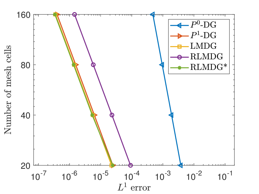
(a) Number of mesh cells.

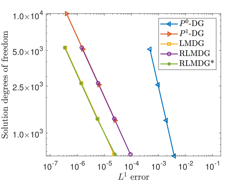
(b) Degrees of freedom.

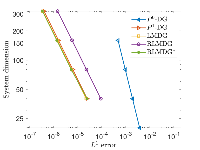
(c) System dimension.

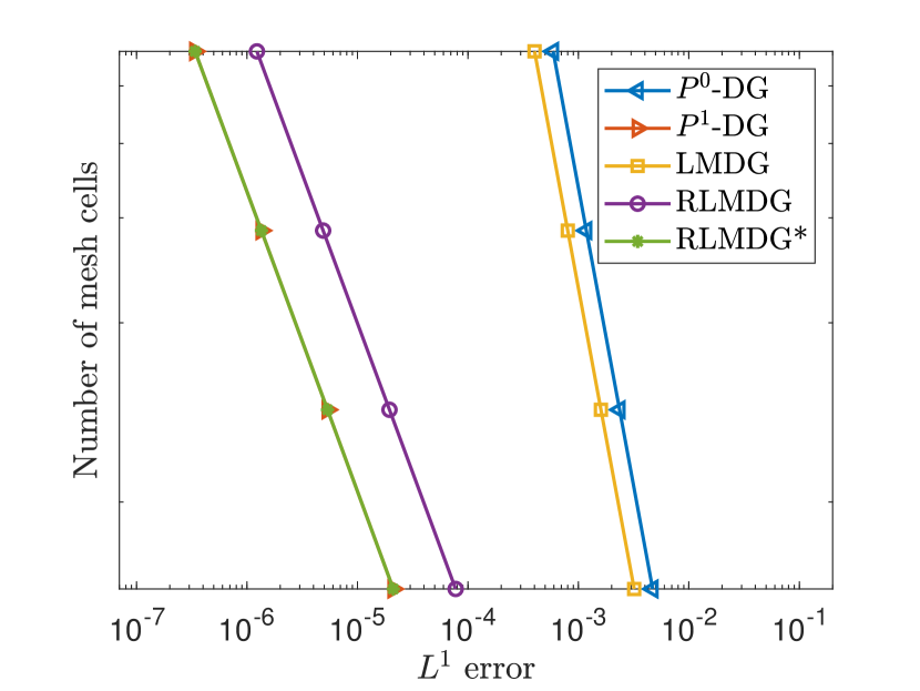
(d) Number of mesh cells.

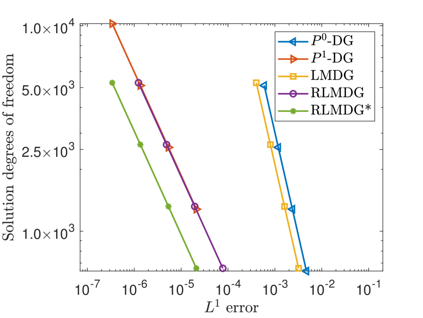
(e) Degrees of freedom.

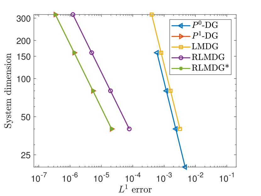
(f) System dimension.

Figure 4.1: Numerical efficiency in Example 4.6. The first row is for isotropic test $\psi=\cos(x)$ and the second row is for anisotropic test $\psi=\cos(x+\mu)$.

To better understand numerical efficiency, we analyze results in Table 4.1 by plotting $L^{1}$ error versus number of mesh cells, total degrees of freedom of the solution (memory costs), and number of equations in the reduced linear system (either (2.14), (3.22), or (3.40)).

For the LMDG method, when the solution is isotropic, the method uses similar number of mesh cells as the $P^{1}$-DG method to reach the same accuracy. As a result, a reduced linear system of similar size is solved, but the degrees of freedom is smaller. For the anisotropic case, the LMDG method is first-order accurate. Compared with the $P^{0}$-DG method, it is able to reach similar accuracy on a coarser mesh. The reduced linear system is larger, but the number of degrees of freedom is indeed smaller.

For the RLMDG method, it seems to be less accurate compared with $P^{1}$-DG method, and a finer mesh has to be used to achieve the same accuracy. As a result, the solution degrees of freedom is similar to that of the $P^{1}$-DG method but the reduced system is even larger. However, we point out a more accurate reconstruction may solve this problem. For example, instead of using two cells, one can recover slopes in the interior region with a three-cell upwind reconstruction (which we call RLMDG^∗). This new method is still second-order accurate, but its error is comparable to the $P^{1}$-DG method and significantly smaller than the current RLMDG method. Efficiency results for RLMDG^∗ are depicted by green lines in Figure 4.1 (they overlap with red lines in (d) and (f)). These results show that RLMDG^∗ yields reduced systems of similar size to those of the $P^{1}$-DG method, but it uses less overall memory.

Example 4.2.

In the second numerical test, we examine the convergence rate and asymptotic preserving property of the methods. Let $\sigma_{\mathrm{s}}=\sigma_{\mathrm{a}}=1$ in (4.1). The computational domain is set as $D=[0,{\pi}]$. We take $\psi_{l}=\psi_{r}=0$ and $q=\frac{4}{3}\sin(x)$. The $32$-point Gauss quadrature is used for $S_{N}$ discretization.

Numerical error at $\varepsilon=10^{-5}$ and $\varepsilon=1$ is listed in Table 4.2, respectively. The reference solutions are set as the numerical solutions with $P^{1}$-DG scheme on a mesh with $1280$ cells. One can see from Table 4.2, the LMDG scheme exhibits second-order convergence rate at $\varepsilon=10^{-5}$, when the solution is almost isotropic, while it converges at a first-order rate when $\varepsilon=1$. The RLMDG method is second-order in both cases.

Solution profiles of different schemes on a sparse uniform mesh, with $h=\pi/8$, are shown in Figure 4.3. When $\varepsilon=10^{-5}$, both LMDG and RLMDG methods preserve the correct diffusion limit, unlike the $P^{0}$-DG method. When $\varepsilon=1$, all schemes give valid approximations.

		$P^{0}$-DG		$P^{1}$-DG		LMDG		RLMDG
$\varepsilon$	$h$	error	order	error	order	error	order	error	order
$10^{-5}$	$1/20$	2.00e-0	-	1.89e-3	-	1.89e-3	-	7.52e-3	-
	$1/40$	2.00e-0	0.00	4.70e-4	2.01	4.71e-4	2.00	1.88e-3	2.00
	$1/80$	2.00e-0	0.00	1.17e-4	2.01	1.16e-4	2.03	4.70e-4	2.00
	$1/160$	1.99e-0	0.00	2.91e-5	2.00	3.06e-5	1.92	1.17e-4	2.00
$1$	$1/20$	1.06e-1	-	2.91e-3	-	3.08e-2	-	9.55e-3	-
	$1/40$	5.38e-2	0.98	7.72e-4	1.92	1.59e-2	0.95	2.60e-3	1.88
	$1/80$	2.71e-2	0.99	1.99e-4	1.95	8.09e-3	0.98	6.90e-4	1.91
	$1/160$	1.35e-2	1.00	5.03e-5	1.99	4.08e-3	0.99	1.80e-4	1.94

Table 4.2: Accuracy test for Example 4.2.

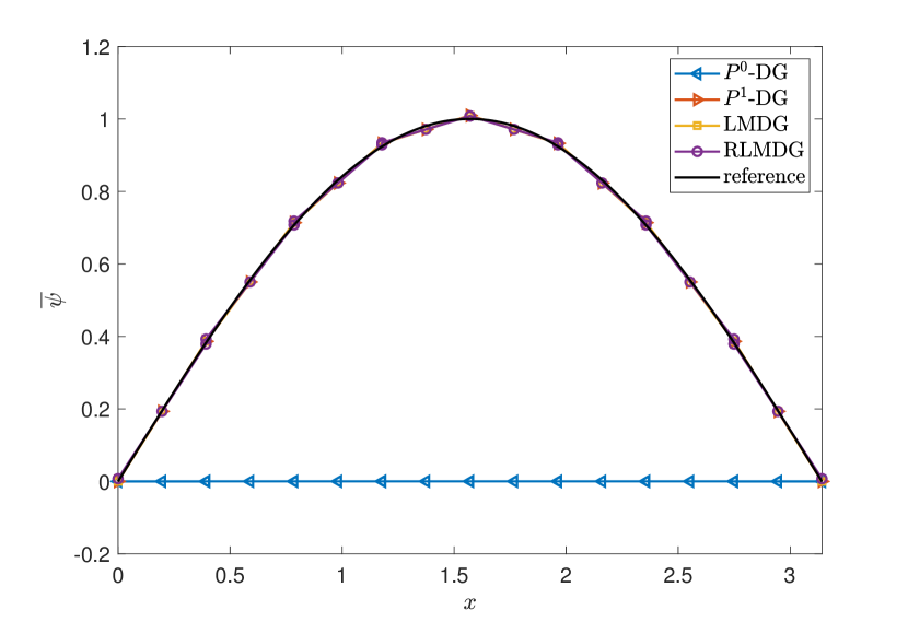
(a) $\varepsilon=10^{-5}$.

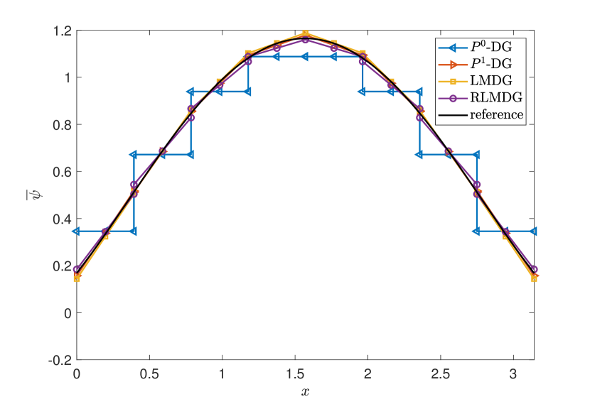
(b) $\varepsilon=1$.

Figure 4.2: Profiles of numerical scalar fluxes in Example 4.2.

Example 4.3.

We then consider a test from [28] with discontinuous cross-sections. The problem is defined on $[0,1]$ and is purely scattering, i.e., $\sigma_{\mathrm{a}}\equiv 0$. The cross-section is $\sigma_{\mathrm{s}}=\sigma_{\mathrm{s,1}}=100$ on the left part of the domain $[0,0.5]$, and is $\sigma_{\mathrm{s}}=\sigma_{\mathrm{s,2}}=100,1000\text{ or }10000$ on the right part $[0.5,1]$. The source term is constant $q=0.01$. In the numerical test, we set the mesh size to be $h=0.1$ and $h=0.02$, and solutions are depicted in Figure 4.3 and Figure 4.4, respectively. As one can see, unlike the $P^{0}$-DG scheme, both LMDG and RLMDG schemes provide correct solution profiles. Since the problem is diffusive, the LMDG scheme gives accurate approximations that are almost indistinguishable with the $P^{1}$-DG solutions. The reconstructed scheme has difficulty resolving the kink at $x=0.5$, likely because the reconstruction is no longer accurate at this point. This artifact can indeed be alleviated as the mesh is refined comparing Figure 4.3 and Figure 4.4.

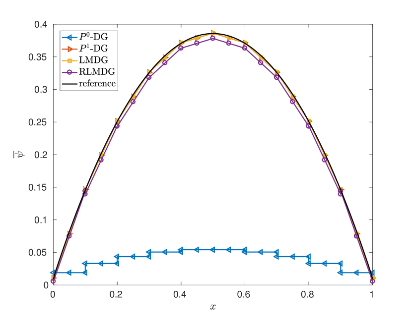
(a) $\sigma_{\mathrm{s,2}}=100$.

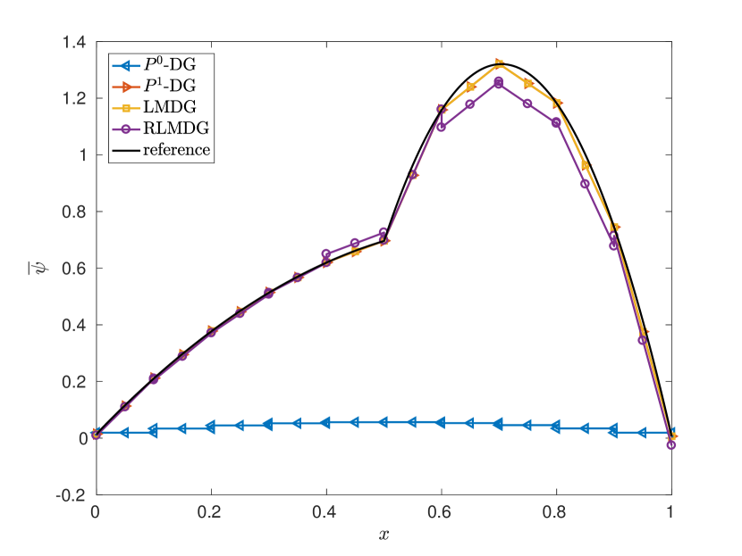
(b) $\sigma_{\mathrm{s,2}}=1000$.

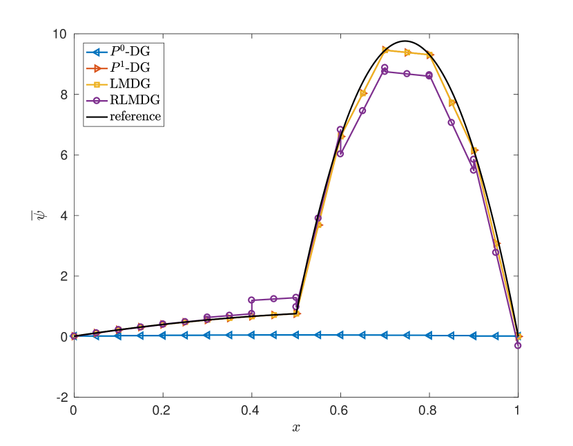
(c) $\sigma_{\mathrm{s,2}}=10000$.

Figure 4.3: Profiles of numerical scalar fluxes in Example 4.3, $h=0.1$.

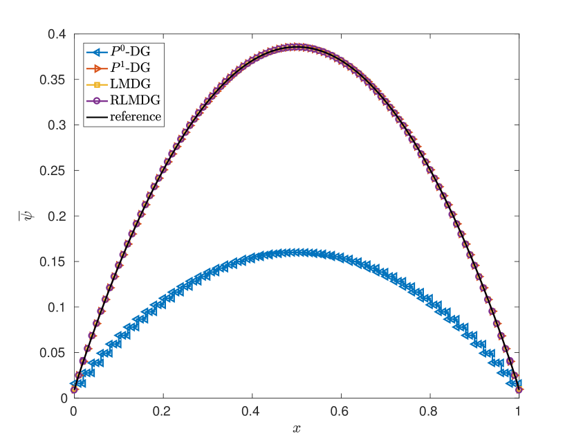
(a) $\sigma_{\mathrm{s,2}}=100$.

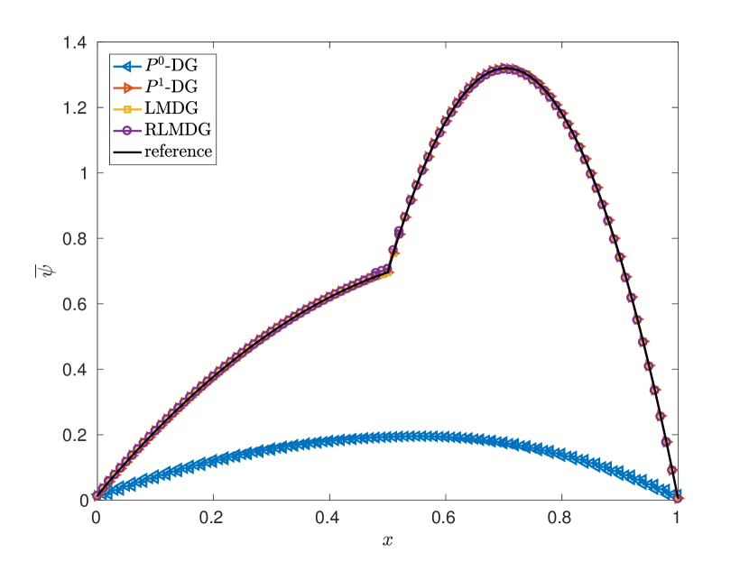
(b) $\sigma_{\mathrm{s,2}}=1000$.

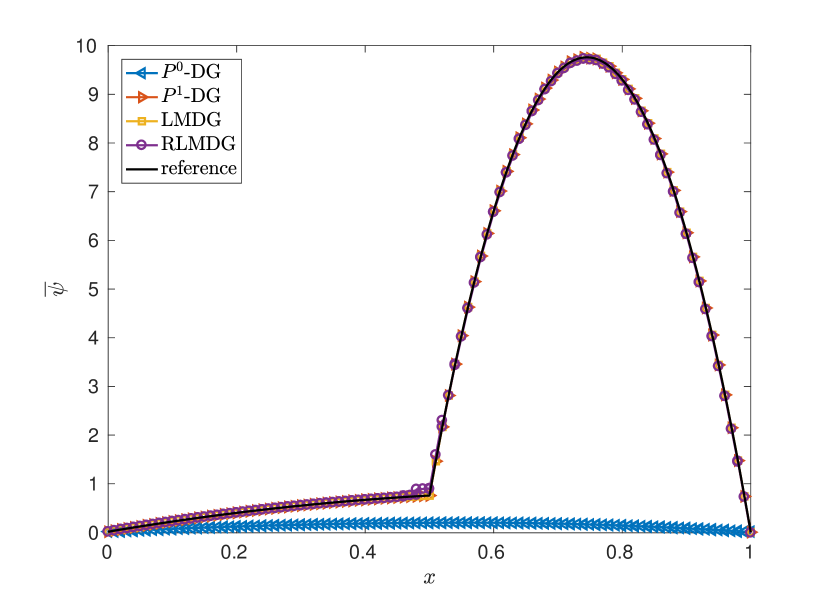
(c) $\sigma_{\mathrm{s,2}}=10000$.

Figure 4.4: Profiles of numerical scalar fluxes in Example 4.3, $h=0.02$.

Example 4.4.

In this numerical test, we solve a test problem from [21] with discontinuous cross-sections. We take $q=0$ with the left inflow $\psi_{l}=1$ at $x_{a}=0$ and $\psi_{r}=0$ at $x_{b}=11$. Let $\frac{\sigma_{\mathrm{s}}}{\varepsilon}=\left\{\begin{matrix}0,&0<x<1\\ 100,&1<x<11\end{matrix}\right.$ and $\varepsilon{\sigma_{\mathrm{a}}}=\left\{\begin{matrix}2,&0<x<1\\ 0,&1<x<11\end{matrix}\right.$. The $16$-point Gauss quadrature rule is used for angular discretization. The spatial mesh is set as $h=\left\{\begin{matrix}0.1,&0<x<1\\ 1,&1<x<11\\ \end{matrix}\right.$.

Profiles of the scalar flux obtained with various schemes are depicted in Figure 4.5(a). The reference solutions are obtained with the $P^{1}$-DG scheme on a refined mesh. The solution of the LMDG scheme is satisfactory. As before, the RLMDG scheme gives an accurate approximation to the scalar flux, except for kinks near the discontinuity. However, this numerical artifact can also be alleviated by suppressing the reconstruction across the discontinuity; see Figure 4.5(b).

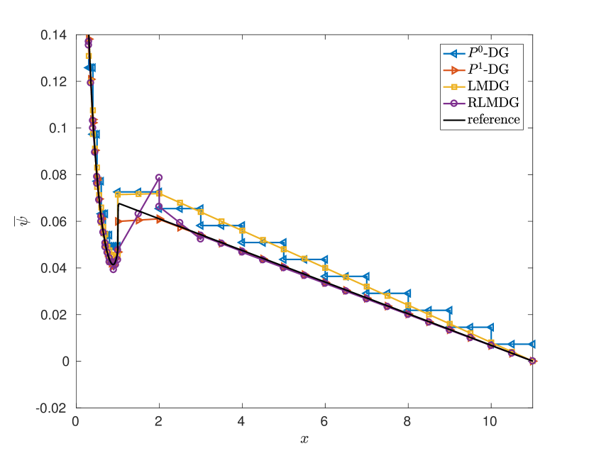
(a) Numerical scalar fluxes.

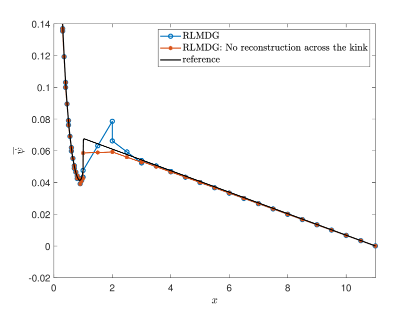
(b) With suppressed reconstruction.

Figure 4.5: Profiles of numerical scalar fluxes in Example 4.4.

Example 4.5.

This test is also from [21], with $D=[0,20]$ and $\psi_{l}=\psi_{r}=0$. The cross-sections are $\frac{\sigma_{\mathrm{s}}}{\varepsilon}=\left\{\begin{matrix}90,&0<x<10\\ 100,&10<x<20\end{matrix}\right.$ and $\varepsilon{\sigma_{\mathrm{a}}}=\left\{\begin{matrix}10,&0<x<10\\ 0,&10<x<20\end{matrix}\right.$. We solve the problem using the ${16}$-point Gauss quadrature rule and the spatial mesh is uniform with $h=1$. For this numerical test, the system has smaller changes among different directions. Both the LMDG and RLMDG schemes give accurate approximations. Solution profiles are give in Figure 4.6.

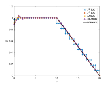
Figure 4.6: Profiles of numerical scalar fluxes in Example 4.5.

4.2 Two dimensional tests

We consider two dimensional problems on Cartesian meshes in this section.

Example 4.6.

We set $\varepsilon=1$ and $\sigma_{\mathrm{s}}=\sigma_{\mathrm{a}}=1$ and test the accuracy with exact solutions $\psi=\sin(x+y)$ and $\psi=(\Omega_{x}-3\Omega_{y})^{2}\sin(2x+y)$. As can be seen from Table 4.3, for $\psi=\sin(x+y)$, both LMDG and RLMDG schemes are second-order accurate. While for the anisotropic problem with $\psi=(\Omega_{x}-3\Omega_{y})^{2}\sin(2x+y)$, the RLMDG scheme is still second-order accurate and the LMDG scheme is first-order accurate.

$\psi=\sin(x+y)$
	$P^{0}$-DG		$P^{1}$-DG		$Q^{1}$-DG		LMDG		RLMDG
$h/\sqrt{2}$	error	order	error	order	error	order	error	order	error	order
$1/20$	2.04e-2	-	1.45e-4	-	1.40e-4	-	1.24e-4	-	4.59e-4	-
$1/40$	1.10e-2	0.89	3.42e-5	2.08	3.53e-5	1.98	3.12e-5	1.99	1.18e-4	1.96
$1/80$	5.77e-3	0.94	8.28e-6	2.04	8.88e-6	1.99	7.82e-6	2.00	2.98e-5	1.98
$1/160$	2.96e-3	0.96	2.04e-6	2.02	2.26e-6	2.00	1.96e-6	2.00	7.51e-6	1.99
$\psi=(\Omega_{x}-2\Omega_{y})^{2}\sin(2x+y)$
	$P^{0}$-DG		$P^{1}$-DG		$Q^{1}$-DG		LMDG		RLMDG
$h/\sqrt{2}$	error	order	error	order	error	order	error	order	error	order
$1/20$	7.84e-2		1.64e-3	-	1.39e-3	-	5.04e-2	-	4.81e-3	-
$1/40$	4.18e-2	0.91	4.12e-4	2.00	3.53e-4	1.98	2.57e-2	0.97	1.21e-3	1.99
$1/80$	2.12e-2	0.98	1.01e-4	2.03	8.87e-5	1.99	1.30e-2	0.99	3.05e-4	1.99
$1/160$	1.07e-2	0.97	2.52e-5	2.00	2.22e-5	2.00	6.51e-3	0.99	7.63e-5	2.00

Table 4.3: 2D accuracy test with fabricated solutions.

Example 4.7.

To examine the asymptotic preserving property, we consider the problem defined on $[-1,1]\times[-1,1]$ with zero inflow boundary conditions. Let $\sigma_{\mathrm{s}}=\sigma_{\mathrm{a}}=1$. We assume $q=(\frac{\pi^{2}}{6}+1)\cos(\frac{\pi}{2}x)\cos(\frac{\pi}{2}y)$. The asymptotic solution is $\psi^{(0)}=\cos(\frac{\pi}{2}x)\cos(\frac{\pi}{2}y)$. We test with $\varepsilon=1,2^{-6},2^{-10},2^{-14}$; the numerical results are given in Figure 4.7. For the $P^{0}$-DG and $P^{1}$-DG schemes, solutions become zero near the diffusion limit, while for the $Q^{1}$-DG scheme, LMDG scheme and RLMDG scheme, the correct asymptotic profile is maintained.

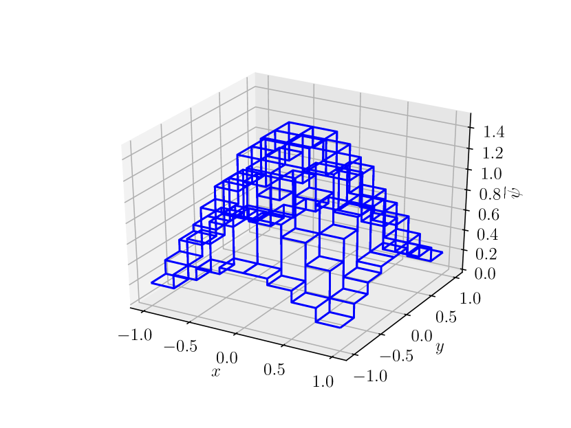
(a) $P^{0}$, $\varepsilon=1$.

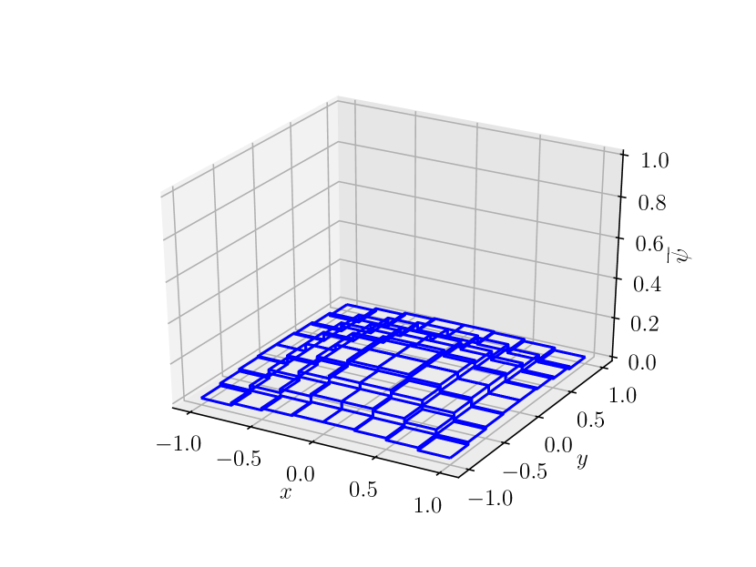
(b) $P^{0}$, $\varepsilon=2^{-6}$.

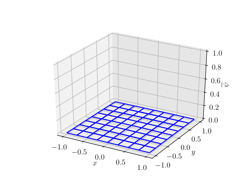
(c) $P^{0}$, $\varepsilon=2^{-10}$.

(d) $P^{0}$, $\varepsilon=2^{-14}$.

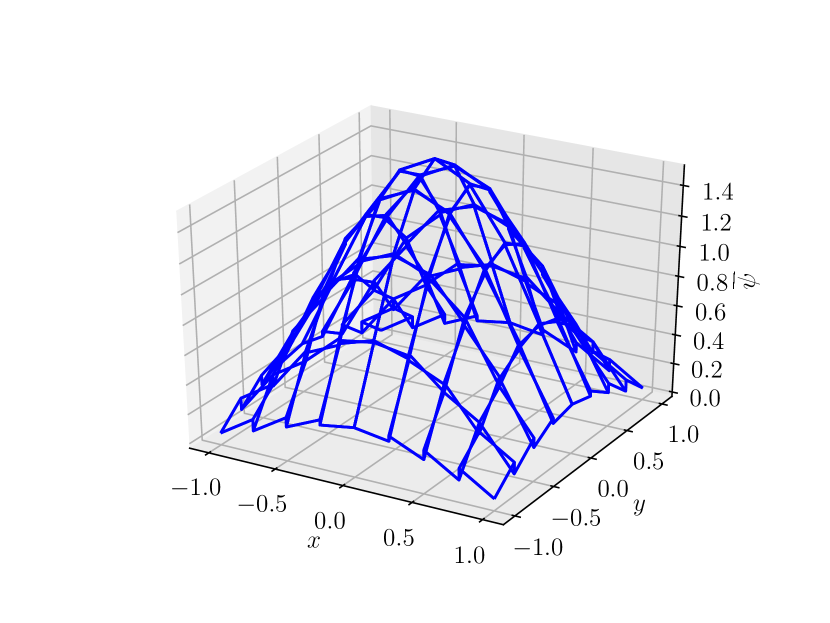
(e) $P^{1}$, $\varepsilon=1$.

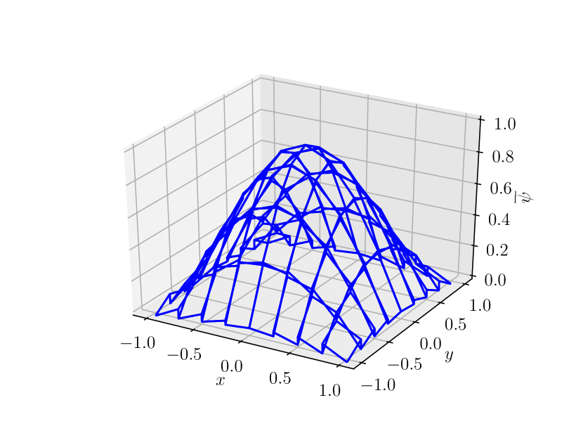
(f) $P^{1}$, $\varepsilon=2^{-6}$.

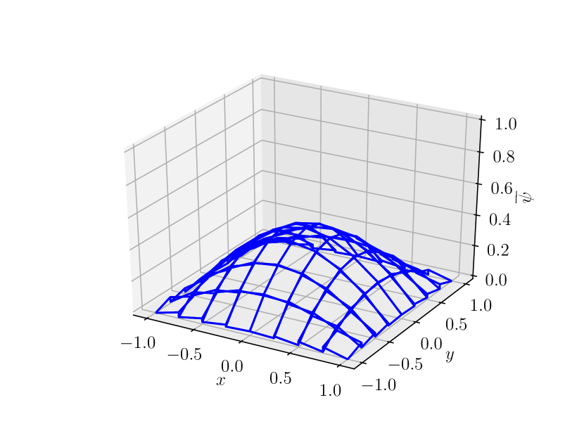
(g) $P^{1}$, $\varepsilon=2^{-10}$.

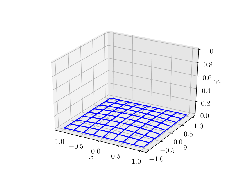
(h) $P^{1}$, $\varepsilon=2^{-14}$.

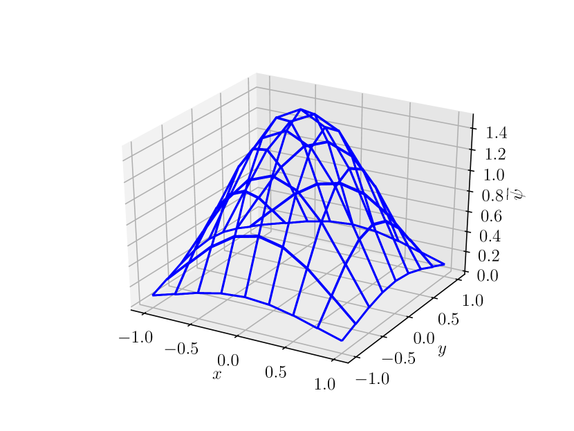
(i) $Q^{1}$, $\varepsilon=1$.

(j) $Q^{1}$, $\varepsilon=2^{-6}$.

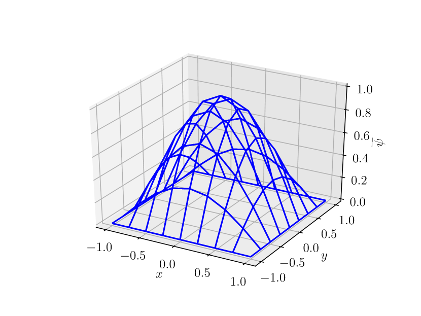
(k) $Q^{1}$, $\varepsilon=2^{-10}$.

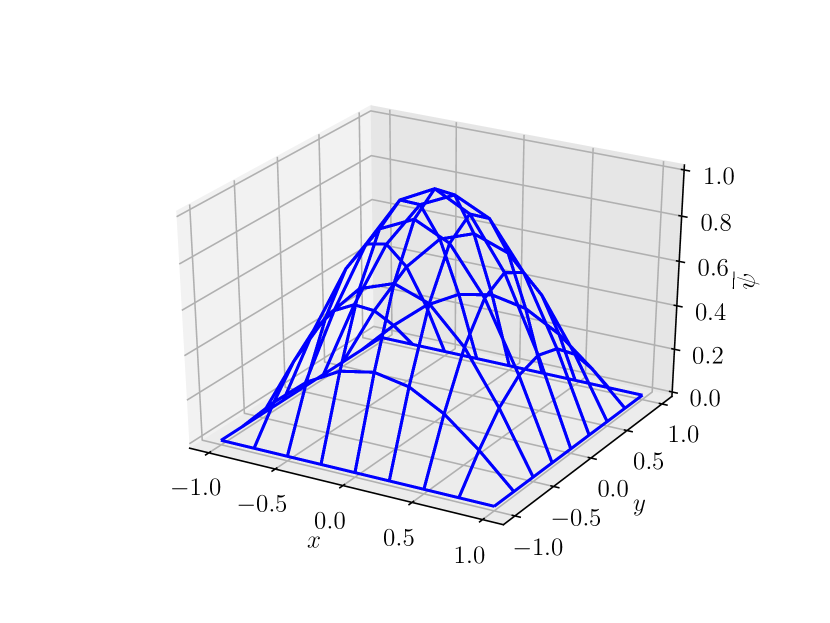
(l) $Q^{1}$, $\varepsilon=2^{-14}$.

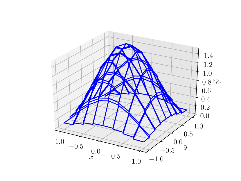
(m) LM, $\varepsilon=1$.

(n) LM, $\varepsilon=2^{-6}$.

(o) LM, $\varepsilon=2^{-10}$.

(p) LM, $\varepsilon=2^{-14}$.

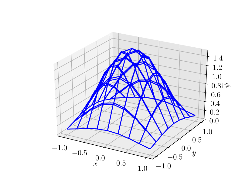
(q) RLM, $\varepsilon=1$.

(r) RLM, $\varepsilon=2^{-6}$.

(s) RLM, $\varepsilon=2^{-10}$.

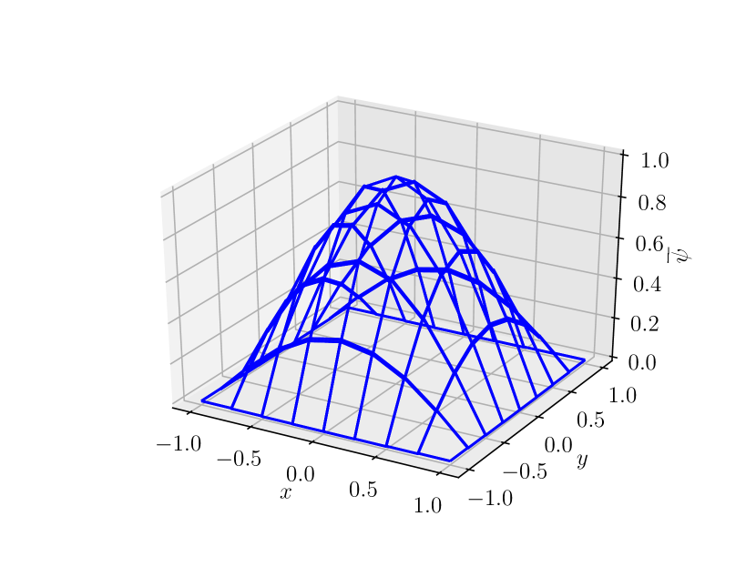
(t) RLM, $\varepsilon=2^{-14}$.

Figure 4.7: Profiles of numerical scalar fluxes in Example 4.7.

5 Conclusions and future work

In this paper, we study a class of low-memory $S_{N}$-DG methods for the radiative transport equation. In our first method, we use the variational form of the original $S_{N}$-DG scheme with a smaller finite element space, in which functions have isotropic slopes. This method preserves the asymptotic diffusion limit and can still be solved with sweeps. It is first-order accurate and exhibits second-order convergence rate near the diffusion limit. The second method is a correction of the first method with reconstructed slopes, which also preserves the diffusion limit and is second-order accurate in general settings (numerically). A summary of different methods and their properties can be found in Table 5.1.

Future work will focus on the efficiency boost of the low-memory methods. Possible directions include: (i) further reducing degrees of freedom by enriching piecewise constant space only with continuous linear elements; (ii) developing preconditioners for linear systems; (iii) comparing numerical efficiency of the methods with different reconstruction approaches, including adaptivity.

		$P^{0}$-DG	$P^{1}$-DG	$Q^{1}$-DG	LMDG	RLMDG
Unisolvency when $\sigma_{\mathrm{a}}\geq\delta_{\mathrm{a}}>0$		Yes				Unknown. Numeri- cally: Yes
Preserves interior diffusion limit	1D	No	Yes
	2D		Triangular: Yes Rectangular: No	Yes
Order of accuracy	isotropic	1	2		2	2
	anisotropic				1
System dimension	1D	$n_{x}$	$2n_{x}$
	2D		$3n_{x}$	$4n_{x}$
	3D		$4n_{x}$	$8n_{x}$
Solution dimension	1D	$n_{\Omega}\cdot n_{x}$	$2n_{\Omega}\cdot n_{x}$		$n_{\Omega}\cdot n_{x}+n_{x}$
	2D		$3n_{\Omega}\cdot n_{x}$	$4n_{\Omega}\cdot n_{x}$	$n_{\Omega}\cdot n_{x}+3n_{x}$
	3D		$4n_{\Omega}\cdot n_{x}$	$8n_{\Omega}\cdot n_{x}$	$n_{\Omega}\cdot n_{x}+7n_{x}$

Table 5.1: Comparison of different methods.

Appendix A Assembly of the matrices

From the variational form (2.12), we can derive a matrix system $\mathbf{L}\mathbf{\Psi}=\mathbf{S}\mathbf{\Psi}+\mathbf{Q}$. The matrices are defined as $\mathbf{L}=[L^{(l,p,r),(l^{\prime},p^{\prime},r^{\prime})}]_{(n_{\Omega}\cdot n_{x}\cdot n_{P})\times(n_{\Omega}\cdot n_{x}\cdot n_{P})}$, $\mathbf{S}=[S^{(l,p,r),(l^{\prime},p^{\prime},r^{\prime})}]_{(n_{\Omega}\cdot n_{x}\cdot n_{P})\times(n_{\Omega}\cdot n_{x}\cdot n_{P})}$ and
$\mathbf{Q}=[Q^{(l,p,r)}]_{(n_{\Omega}\cdot n_{x}\cdot n_{P})}$, where

(A.1) $$L^{(l,p,r),(l^{\prime},p^{\prime},r^{\prime})}=L(\xi^{l^{\prime},p^{\prime},r^{\prime}},\xi^{l,p,r})=\delta_{ll^{\prime}}w_{l}\sum_{K\in\mathcal{T}_{h}}\left(-\int_{K}b^{p^{\prime},r^{\prime}}\Omega_{l}\cdot\nabla b^{p,r}dx\right.$$

$$\left.+\int_{\partial K}\widehat{b}^{p^{\prime},r^{\prime}}\Omega_{l}\cdot\nu_{K}(b^{p,r})^{\mathrm{int}}dx+\int_{K}\left(\frac{\sigma_{s}}{\varepsilon}+\varepsilon\sigma_{a}\right)b^{p^{\prime},r^{\prime}}b^{p,r}dx\right),$$

(A.2) $$S^{(l,p,r),(l^{\prime},p^{\prime},r^{\prime})}=S(\xi^{l^{\prime},p^{\prime},r^{\prime}},\xi^{l,p,r})=w_{l}w_{l^{\prime}}\sum_{K\in\mathcal{T}_{h}}\int_{K}\frac{\sigma_{s}}{\varepsilon}b^{p,r}b^{p^{\prime},r^{\prime}}dx,$$

(A.3) $$Q^{(l,p,r)}=Q(\xi^{l,p,r})=w_{l}\left(\sum_{K\in\mathcal{T}_{h}}\int_{K}\varepsilon qb^{p,r}dx-\sum_{K\in\mathcal{T}_{h}}\int_{\partial K\cap F_{h}^{\partial}}\alpha\Omega_{l}\cdot\nu_{K}b^{p,r}dx\right).$$

Note that $\mathbf{S}$ can be decomposed as the product of two matrices $\mathbf{S}=\mathbf{M}\mathbf{P}$, where $\mathbf{M}=[M^{(l,p,r),(p^{\prime\prime},r^{\prime\prime})}]_{(n_{\Omega}\cdot n_{x}\cdot n_{P})\times(n_{x}\cdot n_{P})}$ with $M^{(l,p,r),(p^{\prime\prime},r^{\prime\prime})}=w_{l}\sum_{K\in\mathcal{T}_{h}}\int_{K}\frac{\sigma_{s}}{\varepsilon}b^{p,r}b^{p^{\prime\prime},r^{\prime\prime}}dx$, and $\mathbf{P}=[P^{(p^{\prime\prime},r^{\prime\prime}),(l^{\prime},p^{\prime},r^{\prime})}]_{(n_{x}\cdot n_{P})\times(n_{\Omega}\cdot n_{x}\cdot n_{P})}$ with $P^{(p^{\prime\prime},r^{\prime\prime}),(l^{\prime},p^{\prime},r^{\prime})}=w_{l^{\prime}}\delta_{p^{\prime\prime}p^{\prime}}\delta_{r^{\prime\prime}r^{\prime}}$. Hence the matrix equation becomes $\mathbf{L}\mathbf{\Psi}=\mathbf{M}\mathbf{P}\mathbf{\Psi}+\mathbf{Q}$.

Appendix B Proof of 2.1

Proof B.1.

Since the variational problem of the $S_{N}$-DG method is unisolvent, $\mathbf{L}-\mathbf{M}\mathbf{P}$ is invertible. To show $\mathbf{I}_{n_{x}\cdot n_{P}}-\mathbf{P}\mathbf{L}^{-1}\mathbf{M}$ is invertible, one only needs to check

(B.4) $$(\mathbf{I}_{n_{x}\cdot n_{P}}-\mathbf{P}\mathbf{L}^{-1}\mathbf{M})\mathbf{X}=\mathbf{0}\Rightarrow\mathbf{X}=\mathbf{0}.$$

Indeed, with $(\mathbf{I}_{n_{x}\cdot n_{P}}-\mathbf{P}\mathbf{L}^{-1}\mathbf{M})\mathbf{X}=\mathbf{0}$, we have

(B.5) $$(\mathbf{L}-\mathbf{M}\mathbf{P})(\mathbf{L}^{-1}\mathbf{M}\mathbf{X})=\mathbf{0} \Rightarrow\mathbf{L}^{-1}\mathbf{M}\mathbf{X}=\mathbf{0}\Rightarrow\mathbf{M}\mathbf{X}=\mathbf{0}\Rightarrow\mathbf{X}=\mathbf{0}.$$

Hence $\mathbf{I}_{n_{x}\cdot n_{P}}-\mathbf{P}\mathbf{L}^{-1}\mathbf{M}$ is invertible.

Appendix C Proof of 3.3

Proof C.1.

Note $\mathbf{B}_{11}$ corresponds to the variational problem (3.1) with $\mathcal{W}_{h}=\mathcal{V}_{h,1}$. Since the variational problem is unisolvent (even when $\sigma_{\mathrm{a}}=0$), $\mathbf{B}_{11}$ is invertible.

$\forall u,v\in\overline{\mathcal{V}}_{h,1}$, since $u=\overline{u}$, we have

(C.6) $$\sum_{j=1}^{n_{\Omega}}w_{j}\int_{K}u_{j}\Omega_{j}\cdot\nabla v_{j}dx=\int_{K}\bar{u}\left(\sum_{j=1}^{n_{\Omega}}w_{j}\Omega_{j}\right)\cdot\nabla\bar{v}dx =0,$$

(C.7) $$\sum_{j=1}^{n_{\Omega}}\sum_{K\in\mathcal{T}_{h}}\int_{K}\frac{\sigma_{\mathrm{s}}}{\varepsilon}(u_{j}-\overline{u})v_{j}dx =0.$$

Therefore,

(C.8) $$B_{11}(u,v)=\sum_{K\in\mathcal{T}_{h}}\int_{K}\varepsilon\sigma_{\mathrm{a}}\overline{u}\ \overline{v}dx+\sum_{j=1}^{n_{\Omega}}w_{j}\sum_{K\in\mathcal{T}_{h}}\int_{\partial K}\Omega_{j}\cdot\nu_{K}\widehat{u}_{j}v_{j}^{\mathrm{int}}dx.$$

We would like to write the last term as a summation with respect to edges. $\nu_{F}^{+}$ is defined as the unit normal of an edge $F$ such that $e_{1}\cdot\nu_{F}^{+}>0$. $e_{1}$ is the vector in $\mathbb{R}^{d}$, whose first component is $1$ and others are $0$. Suppose $\nu_{F}^{+}$ is pointing from $K^{+}$ to $K^{-}$, we denote by $[v]_{j}=v_{j}|_{K^{+}}-v_{j}|_{K^{-}}$. Then

(C.9) $$\sum_{j=1}^{n_{\Omega}}w_{j}\sum_{K\in\mathcal{T}_{h}}\int_{\partial K}\Omega_{j}\cdot\nu\widehat{u}_{j}v_{j}dx =\sum_{j=1}^{n_{\Omega}}w_{j}\sum_{F\in\mathcal{F}_{h}}\int_{F}\Omega_{j}\cdot\nu_{F}^{+}\widehat{u}_{j}[v]_{j}dx$$

$$=\sum_{\begin{subarray}{c}j=1,\dots,n_{\Omega},\\ \Omega_{j}\cdot e_{1}>0\end{subarray}}w_{j}\sum_{F\in\mathcal{F}_{h}}\int_{F}|\Omega_{j}\cdot\nu_{F}^{+}|[u]_{j}[v]_{j}dx.$$

The last equality uses the central symmetry of the angular quadrature. Hence

(C.10) $$B_{11}(u,v)=\sum_{K\in\mathcal{T}_{h}}\int_{K}\varepsilon\sigma_{\mathrm{a}}\overline{u}\ \overline{v}d\Omega_{N}dx+\sum_{\begin{subarray}{c}j=1,\dots,n_{\Omega}\\ \Omega_{j}\cdot e_{1}>0\end{subarray}}w_{j}\sum_{F\in\mathcal{F}_{h}}\int_{F}|\Omega_{j}\cdot\nu_{F}^{+}|[u]_{j}[v]_{j}dx.$$

Here $\Omega_{j}\cdot e_{1}$ gives the first component of $\Omega_{j}$. Since $B_{11}$ is a symmetric and positive semi-definite bilinear form, $\mathbf{B}_{11}$ is then a symmetric and positive semi-definite matrix. The positive definiteness is implied by the fact $\mathbf{B}_{11}$ is invertible.

Appendix D Proof of 3.4

We first prove the following lemma.

Lemma D.1.

Suppose $\mathbf{I}_{m}-\mathbf{C}\mathbf{A}-\mathbf{D}\mathbf{B}$ is invertible, where $\mathbf{A}$ is an $n\times m$ matrix, $\mathbf{B}$ is an $n^{\prime}\times m$ matrix, $\mathbf{C}$ is an $m\times n$ matrix, and $\mathbf{D}$ is an $m\times n^{\prime}$ matrix. Then $\mathbf{I}_{n+n^{\prime}}-\left[\begin{matrix}\mathbf{A}\\ \mathbf{B}\end{matrix}\right]\left[\begin{matrix}\mathbf{C}&\mathbf{D}\end{matrix}\right]$ is invertible.

Proof D.1.

It suffices to show that $\left(\mathbf{I}_{n+n^{\prime}}-\left[\begin{matrix}\mathbf{A}\\ \mathbf{B}\end{matrix}\right]\left[\begin{matrix}\mathbf{C}&\mathbf{D}\end{matrix}\right]\right)\left[\begin{matrix}\mathbf{X}_{0}\\ \mathbf{X}_{1}\end{matrix}\right]=\mathbf{0}$ implies $\mathbf{X}_{0}$ and $\mathbf{X}_{1}$ are $\mathbf{0}$. Indeed, with $\mathbf{X}=\mathbf{C}\mathbf{X}_{0}+\mathbf{D}\mathbf{X}_{1}$, the equality gives

(D.11) $$\mathbf{A}\mathbf{X}=\mathbf{A}\mathbf{C}\mathbf{X}_{0}+\mathbf{A}\mathbf{D}\mathbf{X}_{1}=\mathbf{X}_{0}\quad\text{and}\quad\mathbf{B}\mathbf{X}=\mathbf{B}\mathbf{C}\mathbf{X}_{0}+\mathbf{B}\mathbf{D}\mathbf{X}_{1}=\mathbf{X}_{1},$$

which implies $(\mathbf{I}_{m}-\mathbf{C}\mathbf{A}-\mathbf{D}\mathbf{B})\mathbf{X}=\mathbf{X}-\mathbf{C}\mathbf{X}_{0}-\mathbf{D}\mathbf{X}_{1}=\mathbf{0}$. Since $\mathbf{I}_{m}-\mathbf{C}\mathbf{A}-\mathbf{D}\mathbf{B}$ is invertible, $\mathbf{X}=\mathbf{0}$. Using (D.11) we have $\mathbf{X}_{0}=\mathbf{A}\mathbf{X}=\mathbf{0}$ and $\mathbf{X}_{1}=\mathbf{B}\mathbf{X}=\mathbf{0}$.

Then we show $\mathbf{K}$ is invertible.

Proof D.2.

One can see from 3.1 that the variational problem (3.16) is uniquely solvable. Therefore the associated system (3.21) is also unisolvent and $\mathbf{I}_{n_{\Omega}\cdot n_{x}}-\mathbf{L}_{00}^{-1}\mathbf{M}_{0}\mathbf{P}_{0}-\mathbf{L}_{00}^{-1}\mathbf{L}_{01}\mathbf{\Sigma}^{T}\mathbf{B}_{11}^{-1}\mathbf{\Sigma}\mathbf{L}_{10}$ is invertible. Taking $\mathbf{A}=\mathbf{P}_{0}$, $\mathbf{B}=\mathbf{\Sigma}\mathbf{L}_{10}$, $\mathbf{C}=\mathbf{L}_{00}^{-1}\mathbf{M}_{0}$ and $\mathbf{D}=\mathbf{L}_{00}^{-1}\mathbf{L}_{01}\mathbf{\Sigma}^{T}\mathbf{B}_{11}^{-1}$ in D.1, one can show that the matrix $\mathbf{I}_{n_{x}\cdot n_{P}}-\left[\begin{matrix}\mathbf{P}_{0}\\ \mathbf{\Sigma}\mathbf{L}_{10}\end{matrix}\right]\left[\begin{matrix}\mathbf{L}_{00}^{-1}\mathbf{M}_{0}&\mathbf{L}_{00}^{-1}\mathbf{L}_{01}\mathbf{\Sigma}^{T}\mathbf{B}_{11}^{-1}\end{matrix}\right]$is invertible. Hence $\mathbf{K}=\left(\mathbf{I}_{n_{x}\cdot n_{P}}-\left[\begin{matrix}\mathbf{P}_{0}\\ \mathbf{\Sigma}\mathbf{L}_{10}\end{matrix}\right]\left[\begin{matrix}\mathbf{L}_{00}^{-1}\mathbf{M}_{0}&\mathbf{L}_{00}^{-1}\mathbf{L}_{01}\mathbf{\Sigma}^{T}\mathbf{B}_{11}^{-1}\end{matrix}\right]\right)\left[\begin{matrix}\mathbf{I}_{n_{x}}&\\ &\mathbf{B}_{11}\\ \end{matrix}\right]$is also invertible.

References

- [1] M. L. Adams, Discontinuous finite element transport solutions in thick diffusive problems, Nucl. Sci. Engrg., 137 (2001), pp. 298–333.
- [2] V. Agoshkov, Boundary Value Problems for Transport Equations, Springer Science & Business Media, 2012.
- [3] D. N. Arnold, F. Brezzi, B. Cockburn, and L. D. Marini, Unified analysis of discontinuous Galerkin methods for elliptic problems, SIAM J. Numer. Anal., 39 (2002), pp. 1749–1779.
- [4] I. Babuška and M. Suri, On locking and robustness in the finite element method, SIAM J. Numer. Anal., 29 (1992), pp. 1261–1293.
- [5] C. Bardos, R. Santos, and R. Sentis, Diffusion approximation and computation of the critical size, Trans. Amer. Math. Soc., 284 (1984), pp. 617–649.
- [6] A. Bensoussan, J. L. Lions, and G. C. Papanicolaou, Boundary layers and homogenization of transport processes, Publ. Res. Inst. Math. Sci., 15 (1979), pp. 53–157.
- [7] B. Cockburn and C.-W. Shu, Runge–Kutta discontinuous Galerkin methods for convection-dominated problems, J. Sci. Comput., 16 (2001), pp. 173–261.
- [8] R. Dautray and J. L. Lions, Mathematical Analysis and Numerical Methods for Science and Technology, Volume 6: Evolution Problems II, Spinger-Verlag, Berlin, 2000.
- [9] B. Davison, Neutron Transport Theory, Oxford University Press, London, 1973.
- [10] H. Egger and M. Schlottbom, A mixed variational framework for the radiative transfer equation, Mathematical Models and Methods in Applied Sciences, 22 (2012), p. 1150014.
- [11] G. H. Golub and C. F. Van Loan, Matrix Computations, Johns Hopkins University Press, 3 ed., 2012.
- [12] F. Graziani, Computational Methods in Transport, vol. 48, Springer, 2006.
- [13] J.-L. Guermond and G. Kanschat, Asymptotic analysis of upwind discontinuous Galerkin approximation of the radiative transport equation in the diffusive limit, SIAM J. Numer. Anal., 48 (2010), pp. 53–78.
- [14] J.-L. Guermond, G. Kanschat, and J. C. Ragusa, Discontinuous Galerkin for the radiative transport equation, in Recent Developments in Discontinuous Galerkin Finite Element Methods for Partial Differential Equations, Springer, 2014, pp. 181–193.
- [15] J.-L. Guermond, B. Popov, and J. Ragusa, Positive asymptotic preserving approximation of the radiation transport equation, arXiv preprint arXiv:1905.03390, (2019).
- [16] G. J. Habetler and B. J. Matkowsky, Uniform asymptotic expansions in transport theory with small mean free paths, and the diffusion approximation, J. Math. Phys., 16 (1975), pp. 846–854.
- [17] W. Han, J. Huang, and J. Eichholz, Discrete-ordinate discontinuous Galerkin methods for solving the radiative transfer equation, SIAM J. Sci. Comput., 32 (2010), pp. 477–497.
- [18] V. Heningburg and C. Hauck, Hybrid solver for the radiative transport equation using finite volume and discontinuous Galerkin, submitted, (2019).
- [19] S. Jin, Efficient asymptotic-preserving (AP) schemes for some multiscale kinetic equations, SIAM J. Sci. Comput., 21 (1999), pp. 441–454.
- [20] S. Jin and C. D. Levermore, Numerical schemes for hyperbolic conservation laws with stiff relaxation terms, J. Comput. Phys., 126 (1996), pp. 449–467.
- [21] E. Larsen and J. Morel, Asymptotic solutions of numerical transport problems in optically thick, diffusive regimes II, J. Comput. Phys., 83 (1989), pp. 212–236.
- [22] E. W. Larsen, J. Morel, and W. F. Miller, Asymptotic solutions of numerical transport problems in optically thick, diffusive regimes, J. Comput. Phys., 69 (1987), pp. 283–324.
- [23] E. W. Larsen and J. E. Morel, Advances in discrete-ordinates methodology, in Nuclear Computational Science, Springer, 2010, pp. 1–84.
- [24] P. Lesaint and P. A. Raviart, On a finite element method for solving the neutron transport equation, in Mathematical Aspects of Finite Elements in Partial Differential Equations, Proceedings of a Symposium Conducted by the Mathematics Research Center, the University of Wisconsin-Madison, Madison, WI, USA, 1974, pp. 1–3.
- [25] E. E. Lewis and J. W. F. Miller, Computational Methods in Neutron Transport, John Wiley and Sons, New York, 1984.
- [26] D. Mihalis and B. Weibel-Mihalis, Foundations of Radiation Hydrodynamics, Dover, Mineola, New York, 1999.
- [27] G. C. Pomraning, Radiation Hydrodynamics, Pergamon Press, New York, 1973.
- [28] J. C. Ragusa, J.-L. Guermond, and G. Kanschat, A robust -DG-approximation for radiation transport in optically thick and diffusive regimes, J. Comput. Phys., 231 (2012), pp. 1947–1962.
- [29] W. H. Reed and T. Hill, Triangular mesh methods for the neutron transport equation, tech. report, Los Alamos Scientific Lab., N. Mex.(USA), 1973.
- [30] L. Wu and Y. Guo, Geometric correction for diffusive expansion of steady neutron transport equation, Commun. Math. Phys., 336 (2015), pp. 1473–1553.
- [31] Y. Xu and C.-W. Shu, Local discontinuous Galerkin methods for high-order time-dependent partial differential equations, Commun. Comput. Phys., 7 (2010), pp. 1–46.
- [32] J. Yan and C.-W. Shu, Local discontinuous Galerkin methods for partial differential equations with higher order derivatives, J. Sci. Comput., 17 (2002), pp. 27–47.