Rare Disease Detection by Sequence Modeling with Generative Adversarial Networks

Abstract

Rare diseases affecting 350 million individuals are commonly associated with delay in diagnosis or misdiagnosis. To improve those patients’ outcome, rare disease detection is an important task for identifying patients with rare conditions based on longitudinal medical claims. In this paper, we present a deep learning method for detecting patients with exocrine pancreatic insufficiency (EPI) (a rare disease). The contribution includes 1) a large longitudinal study using 7 years medical claims from 1.8 million patients including 29,149 EPI patients, 2) a new deep learning model using generative adversarial networks (GANs) to boost rare disease class, and also leveraging recurrent neural networks to model patient sequence data, 3) an accurate prediction with 0.56 PR-AUC which outperformed benchmark models in terms of precision and recall.

1 Introduction

Rare disease affect 350 million patients worldwide (Kaplan et al., 2013). Collectively they are common but individually they are rare. Given rare diseases’ low prevalence rate among population, the low disease awareness could lead to patients being misdiagnosed/undiagnosed and not getting the appropriate treatment. Patients with rare diseases often visit several physicians over the course of many years before they receive diagnoses for their conditions (Boat et al., 2011). An effective detection method is crucial to help raise disease awareness and achieve early disease intervention (Cameron et al., 2010). On the other hand, interest in machine learning for healthcare has grown immensely during last several years (Ching et al., 2018). Several machine learning methods, such as Recurrent Network (Choi et al., 2016c; Lipton et al., 2015), auto encoder (Miotto et al., 2016), FHIR-formatted representation (Rajkomar et al., 2018), etc. have been proposed to predict patient-level disease using electronic healthcare record (EHR) data. For more comprehensive overview of machine learning application on healthcare, we refer readers to (Xiao et al., 2018; Ghassemi et al., 2018; Obermeyer & Emanuel, 2016).

Recently, deep learning based models, such as long short-term memory and attention models, have been widely applied for disease detection and made improvements on prediction accuracy. In (Choi et al., 2016a), the authors proposed an approach for converting the patient history into medical sequence and then train a long short term memory for sequence labeling task, based on which, an application was developed in (Choi et al., 2016c). To enhance the interpretability, there have been great efforts of trying to explain black-box deep models, including via attention mechanism (Choi et al., 2016b, 2017), decay factor citebai2018interpretable, mimic decisions of deep models with decision tree (Che et al., 2016, 2017), etc.

Generative adversarial networks (GANs) (Goodfellow et al., 2014) have drawn numerous attention for its potential to generate almost true samples from random noise inputs. Although the original idea was more focused on the generator, in (Salimans et al., 2016; Dai et al., 2017), the authors proposed to use GANs in a semi-supervised learning (SSL) setting and demonstrated that GANs performed well by leveraging unlabeled data with novel training techniques. Meanwhile, the problem of rare disease detection falls perfectly under the setting of semi-supervised learning. Since the diagnosed patient population is extremely small, we have limited positive samples but a large number of patients who are under-diagnosed.

Instead of using hand-crafted features as input to a classifier (Li et al., 2018), we directly worked with patient medical history sequences. This comes with multiple benefits, including the ability to capture more complex disease patterns, saving extensive efforts in feature engineering, and making the framework easier transferable to another disease. Since GANs were not intrinsically able to handle sequence data, we opted to use recurrent neural network (RNN)-based model for fix-length sequence embedding.

2 Method

The architecture of our framework is shown in Figure 1.

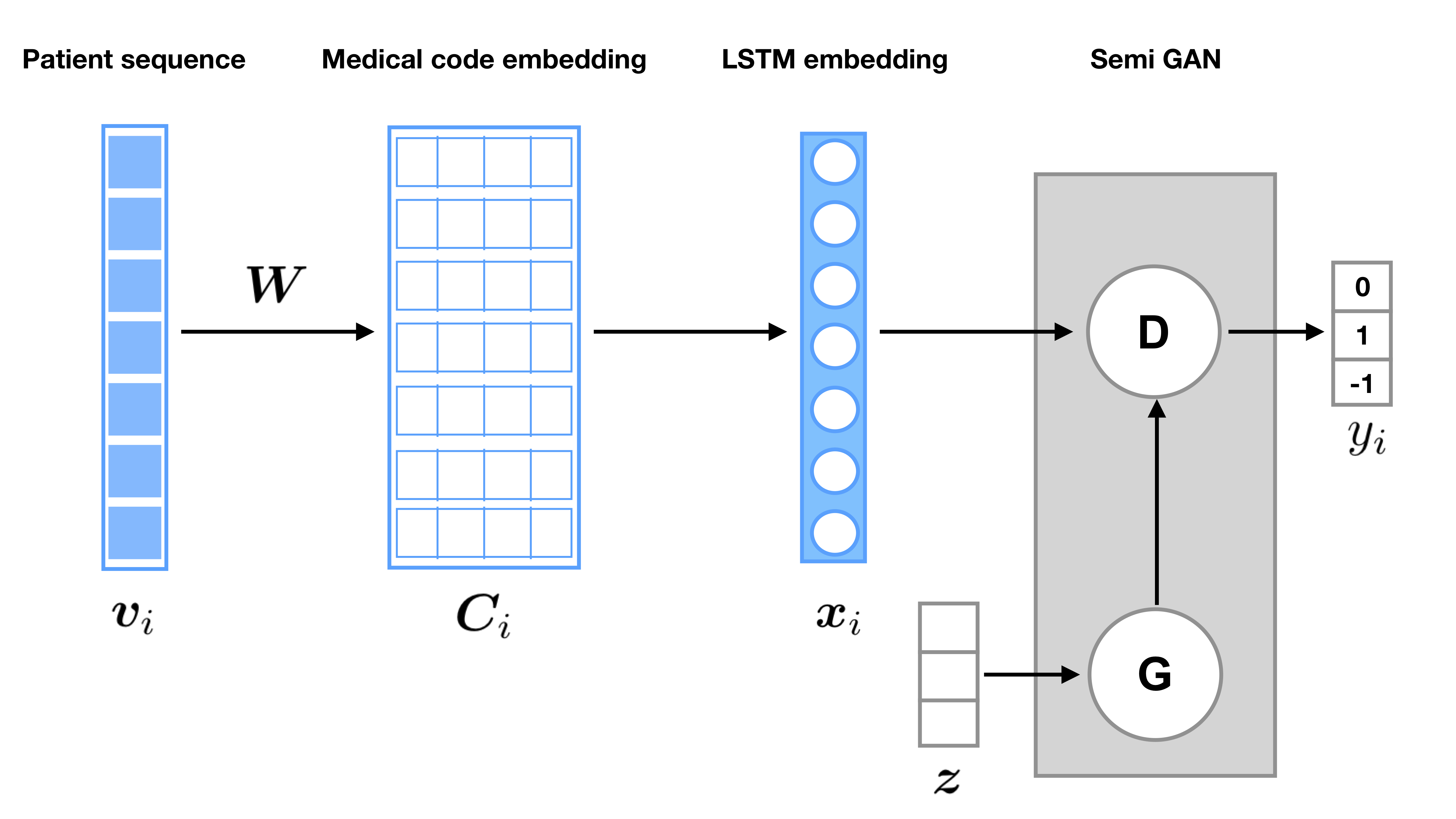
Figure 1: Framework architecture illustrated. $z$ is a random noise input to the generator of GAN.

Each patient is represented by a sequence $\bm{v}_{i}=\{v_{ij},j=1,\dots,N\}$, of which $v_{ij}$ is a medical code indicating a type of hospital visit (Dx) or prescription (Rx). A graphical illustration of such representation is shown in Figure 2. The patient sequence is then transformed to its matrix representation $\bm{C}_{i}$ by embedding the medical codes, i.e. $\bm{c}_{ij}=\bm{W}h(v_{ij})$, where $\bm{W}$ is embedding matrix and $h(\cdot)$ denotes one-hot encoding. Then an LSTM network is used to encode the sequence to $\bm{x}_{i}$. The embedded medical sequence is fed into the discriminator $D$ of a SSL GAN, where the prediction is either positive (1), negative (0) or generated sample by generator $G$ (-1).

Figure 2: A toy example of a patient medical history sequence. Dx refers to diagnosis, Rx refers to prescription and Px refers to medical procedure. The subscripts denote different codes within each category.

2.1 Patient Record Embedding

Encode medical codes. In the patient medical history sequence, each medical code is essentially a categorical variable. The number of categories (different types of medical codes) depends on the level of specificity, i.e., the more specific the meaning of a code is, the more unique codes there would be. In our case, we end up with 5362 unique codes.

We are inspired by the concept of word embedding in natural language processing (NLP) community. Some notable examples include word2vec (Mikolov et al., 2013) and Glove (Pennington et al., 2014). In the original application, the vector representations retain semantic meanings, e.g., synonyms of a word tend to be closer to each other spatially. We will demonstrate a similar behavior of our medical code embedding in a later section.

We used skip-gram model with negative sampling to train the embedding network. The minimum count for valid code is 5, i.e., any codes that occur less than five times in all the sequences would be discarded for training the embedding model, and they were assigned a all-zero vector as their embedding. This left us with 5035, or 93% of all the unique codes. The dimension $d_{w}$ of embedding vector was empirically chosen to be 300.

Embed Longitudinal Records. The most prominent model for processing time series or sequence data is recurrent neural network (RNN). Different variations of memory cells, including long short-term memory (LSTM) (Hochreiter & Schmidhuber, 1997) and gated recurrent unit (GRU) (Chung et al., 2014), were proposed to handle the long-term dependencies over time, which significantly improved the performance of RNNs in various types of tasks, such as sequence classification, sequence tagging (Huang et al., 2015), and machine translation (Cho et al., 2014). A commonly used technique in various tasks is to use the hidden state vector as a representation of the sequence.

We adopted the same idea for sequence embedding. Specifically, patient sequences were padded with a fixed length of $N$. Only labeled training patient sequences were used for training LSTM embedding model. A single-layer LSTM with dimension of the hidden state equal to $d_{S}$ was used. The hidden state of each time stamp was retained, and then aggregated by max pooling operation over time, which resulted in a $d_{S}$-dimension vector. In our experiments, we empirically chose $N=300$ and $d_{S}=256$. After sequence embedding, we appended the patients’ age and gender, and then scale all the features to the range between -1 and 1. The final feature vector has a dimension of 258.

2.2 Semi-supervised GAN

In the original framework of GANs (Goodfellow et al., 2014), a GAN has a generator network $G$ that takes random noise as input and produce samples that follow the real data distribution $p_{data}(x)$. The training of $G$ is guided by the discriminator network $D$, which is trained to distinguish samples from the generator distribution $p_{model}(x)$ from real data. Suppose that the goal of $D$ extends to finding the actual class assignment of real samples and $K$ is the number of possible classes of labeled data, i.e., $p_{D}(y=K+1|x)$ is the probability of a sample generated from $G$. Then the loss function for training $D$ comes from three parts, labeled data $\mathcal{L}$, unlabeled data $\mathcal{U}$ and data from $G$:

$$L_{\mathcal{L}}=-\mathbb{E}_{\bm{x},y\sim\mathcal{L}}\>[\log p_{D}(y|\bm{x},y<K+1)],$$ (1)

$$L_{\mathcal{U}}=-\mathbb{E}_{\bm{x}\sim\mathcal{U}}\>[\log p_{D}(y\leq K|\bm{x})],$$

$$L_{\mathcal{G}}=-\mathbb{E}_{\bm{x}\sim G}\>[\log p_{D}(y=K+1|\bm{x})],$$

And the total discriminator loss becomes $L_{D}=L_{\mathcal{L}}+L_{\mathcal{U}}+L_{\mathcal{G}}$. The first term in Equation 1 is the standard supervised cross-entropy loss, which minimizes the negative log probability of the label, given the data sample is labeled. The second term minimizes the negative log probability of an unlabeled sample coming from one of $K$ possible classes. The third term minimizes the negative probability of a fake sample being recognized.

One thing to note is that the discriminator with $K+1$ outputs is over-parameterized, since the outputs of a softmax function sum to one. Thus, we can set $D$ with $K$ outputs and the equivalent discriminator is given by $\displaystyle D(x)=\frac{Z(x)}{Z(x)+1}$, where $Z(x)=\sum_{k=1}^{K}\exp[l_{k}(x)]$.

In our experiments, we set $D$ and $G$ to have the same architecture but mirroring each other, with five hidden layers. A tanh layer is added at the end of $G$ that maps the output to the range between -1 and 1 (same as input features). We used weight normalization (Salimans & Kingma, 2016) and drop out (Srivastava et al., 2014) to accelerate training and prevent overfitting.

2.3 Training and Inference

Training GANs is notoriously difficult, particularly in a semi-supervised learning setting that requires jointly learning from labeled and unlabeled data. As noted in (Salimans et al., 2016), using feature matching loss for $G$ works well empirically for semi-supervised learning. The objective of feature matching is guiding the generator to generate samples that match the first order statistics of real data. Furthermore, instead of directly minimizing the distance between generated sample mean and real sample mean, the discriminator was used as a feature extractor and the intermediate layer output was used as the ”feature” of data samples. The loss term of feature matching is expressed as

$$L_{FM}=||\mathbb{E}_{\bm{x}\sim G}f(\bm{x})-\mathbb{E}_{\bm{x}\sim\mathcal{U}}f(\bm{x})||^{2}.$$ (2)

A more in-depth discussion of using GANs in semi-supervised learning setting can be found in (Dai et al., 2017). It was suggested that the generator in SSL should generate samples that are complement to real samples. Intuitively, only if the generated sample distribution does not interfere the true sample distributions, it can help the discriminator to learn the manifolds of real samples from different classes. To achieve this, the paper proposed to increase the diversity of generated samples by increasing generator entropy, via introducing a new loss term pull-away term (PT) first proposed in (Zhao et al., 2016):

$$L_{PT}=\frac{1}{N(N-1)}\sum_{i=1}^{N}\sum_{j\neq i}\Big{(}\frac{f(x_{i})^{T}f(x_{j})}{||f(x_{i})||||f(x_{j})||}\Big{)}^{2}.$$ (3)

Additionally, in order for complement generator to work, the discriminator needs to have strong belief on fake-real on unlabeled data. This is achieved by adding a conditional entropy loss to discriminator:

$$L_{ent}=\mathbb{E}_{\bm{x}\sim\mathcal{U}}\sum_{k=1}^{K}p_{D}(k|x)\log p_{D}(k|x).$$ (4)

Finally, the SSL GAN model has discriminator loss $L_{D}=L_{\mathcal{L}}+L_{\mathcal{U}}+L_{\mathcal{G}}+L_{ent}$ and generator loss $L_{G}=L_{FM}+L_{PT}$.

3 Experiment

3.1 Data

We leverage data from IQVIA longitudinal prescription (Rx) and medical claims (Dx) databases, which include hundreds of millions patients’ clinical records. In our study, we focus on one type of rare disease, exocrine pancreatic insufficiency (EPI).

The detailed data preparation process is as follows. We pulled the diagnoses, procedures and prescriptions at transaction level from January 1, 2010 to July 31, 2017. We only kept a subset of patients by applying standard patient eligibility rules, which left us with a total number of 1,792,760 patients. Out of all the patients, 29,149 of them (1.6%) are found to be diagnosed with EPI, which are labeled as positive. 80% of the positive patients were used for training and validation and the rest were held for testing. It is important to note that the remaining patients are under-diagnosed, not essentially negative, so we cannot simply label them as is. Therefore, we applied business rules and identified 69,845 negative patients (three times as the number of positive training patients) for training and validation. The final numbers are shown in Table 1.

	Positive	Negative	Unlabeled
Total	29,149	506,450	1,257,161
Train/validation	23,395	69,845	1,257,161
Test	5,754	436,605	0

Table 1: Population distribution.

3.2 Baseline

For comparison, we chose logistic regression (LR), random forest (RF), XGBoost (XGB) and the discriminator (DNN) in the GAN architecture as baseline models. Note that the input to the benchmark classifiers is the output of LSTM embedding.

3.3 Evaluation Strategy

We used Adam optimizer (Kingma & Ba, 2014) to train each model, with the default learning rate set to 0.001. The number of training epoches was 20. The model was implemented and tested in Tensorflow with GPU support on a system equipped with 128GB RAM, 8 Intel Xeon E5-2683 at 2.10GHz CPUs and one Tesla P100-PCIE GPU.

Because of the high imbalance of data, we used precision-recall (PR) curve and area of PR curve (PR AUC) as evaluation metrics. The PR AUC is computed by trapezoidal rule (Purves, 1992).

4 Result

In this section, we first present some descriptive results on medical code embedding, and then quantitative results of the model performance comparison.

4.1 Embedding visualization

As described in Section 2.1, each medical code was represented as a 300-dimension dense vector. In order to examine whether the embedding vectors retain meaningful medical information, we identified 67 diagnosis (Dx) codes within two therapeutic areas (TAs), respiratory disease and mental disorder, as well as corresponding prescription (Rx) codes. We used t-SNE (Maaten & Hinton, 2008) technique for visualization of the selected codes. The visualization result is shown in Figure 3. We observe that two sets of Rx codes are centered, with each forming its own cluster. The corresponding Dx codes are clustered by their TAs, and aligned with Rx codes on either side.

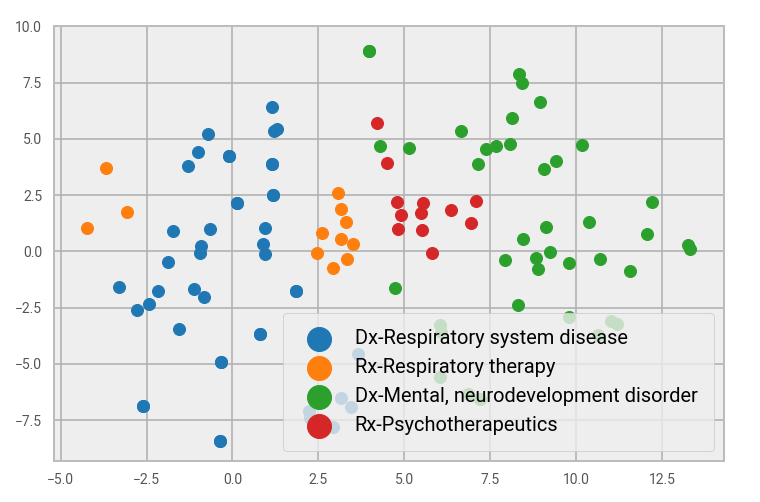
Figure 3: The visualization result by t-SNE of medical codes. Blue and orange dots are respiratory diagnosis (Dx) and prescription (Rx) codes, respectively. The green and red are Dx and Rx codes for mental diseases.

4.2 Model comparison

The PR-AUC by the SSL GAN was 0.56, and the deep neural network with the same architecture as the discriminator had a score of 0.52. We saw a relative increase of 6% over the best benchmark model. The precision-recall curves of all models are shown in Figure 4.

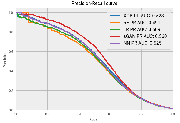
Figure 4: Precision-recall curves of the SSL GAN and benchmark models, where sGAN refers to SSL GAN model.

5 Discussion

The problem of semi-supervised learning often comes with the issue of limited labeled data, and sometimes extreme class imbalance. In our problem of interest, we had both issues. In order to improve the classification performance, it is crucial to fully make use of unlabeled data. By comparing the PR curves, we may cautiously conclude that the performance gain over DNN was from the unlabeled data.

Although the idea of generative adversarial nets is rather straightforward and intriguing, the training process is extremely cumbersome and difficult to reach convergence. According to (Salimans et al., 2016), the training process equals to finding a Nash equilibrium of a non-convex game with continuous, high-dimensional parameters, which may fail to converge if using gradient descent based optimization algorithm (Goodfellow, 2014). Therefore, carefully designed loss functions are crucial to successfully using GAN-based model.

6 Conclusion

In this work, we present a novel framework which combines the merits of both recurrent neural networks and generative adversarial networks. We demonstrated that GANs used in a semi-supervised learning setting can benefit from the vast number of unlabeled data to improve prediction performance, even under an extreme data imbalance scenario. Furthermore, by utilizing RNN-based networks to directly work with patient medical sequences, we are free from extensive work of feature engineering. More importantly, our preliminary analysis of the medical code embedding shows some very interesting properties that are worth investigating in the future. Finally, this framework can be easily transferred to detecting another disease of interest.

References

- Boat et al. (2011) Boat, T. F., Field, M. J., et al. Rare diseases and orphan products: Accelerating research and development. National Academies Press, 2011.
- Cameron et al. (2010) Cameron, M. J., Horst, M., Lawhorne, L. W., and Lichtenberg, P. A. Evaluation of academic detailing for primary care physician dementia education. American Journal of Alzheimer’s Disease & Other Dementias®, 25(4):333–339, 2010.
- Che et al. (2017) Che, C., Xiao, C., Liang, J., Jin, B., Zho, J., and Wang, F. An rnn architecture with dynamic temporal matching for personalized predictions of parkinson’s disease. In Proceedings of the 2017 SIAM International Conference on Data Mining, pp. 198–206. SIAM, 2017.
- Che et al. (2016) Che, Z., Purushotham, S., Khemani, R. G., and Liu, Y. Interpretable deep models for icu outcome prediction. AMIA … Annual Symposium proceedings. AMIA Symposium, 2016:371–380, 2016.
- Ching et al. (2018) Ching, T., Himmelstein, D. S., Beaulieu-Jones, B. K., Kalinin, A. A., Do, B. T., Way, G. P., Ferrero, E., Agapow, P.-M., Zietz, M., Hoffman, M. M., et al. Opportunities and obstacles for deep learning in biology and medicine. Journal of The Royal Society Interface, 15(141):20170387, 2018.
- Cho et al. (2014) Cho, K., Van Merriënboer, B., Bahdanau, D., and Bengio, Y. On the properties of neural machine translation: Encoder-decoder approaches. arXiv preprint arXiv:1409.1259, 2014.
- Choi et al. (2016a) Choi, E., Bahadori, M. T., Schuetz, A., Stewart, W. F., and Sun, J. Doctor ai: Predicting clinical events via recurrent neural networks. In Machine Learning for Healthcare Conference, pp. 301–318, 2016a.
- Choi et al. (2016b) Choi, E., Bahadori, M. T., Sun, J., Kulas, J., Schuetz, A., and Stewart, W. Retain: An interpretable predictive model for healthcare using reverse time attention mechanism. In Advances in Neural Information Processing Systems, pp. 3504–3512, 2016b.
- Choi et al. (2016c) Choi, E., Schuetz, A., Stewart, W. F., and Sun, J. Using recurrent neural network models for early detection of heart failure onset. Journal of the American Medical Informatics Association, 24(2):361–370, 2016c.
- Choi et al. (2017) Choi, E., Bahadori, M. T., Song, L., Stewart, W. F., and Sun, J. Gram: graph-based attention model for healthcare representation learning. In Proceedings of the 23rd ACM SIGKDD International Conference on Knowledge Discovery and Data Mining, pp. 787–795. ACM, 2017.
- Chung et al. (2014) Chung, J., Gulcehre, C., Cho, K., and Bengio, Y. Empirical evaluation of gated recurrent neural networks on sequence modeling. arXiv preprint arXiv:1412.3555, 2014.
- Dai et al. (2017) Dai, Z., Yang, Z., Yang, F., Cohen, W. W., and Salakhutdinov, R. R. Good semi-supervised learning that requires a bad gan. In Advances in neural information processing systems, pp. 6510–6520, 2017.
- Ghassemi et al. (2018) Ghassemi, M., Naumann, T., Schulam, P., Beam, A. L., and Ranganath, R. Opportunities in machine learning for healthcare. arXiv preprint arXiv:1806.00388, 2018.
- Goodfellow et al. (2014) Goodfellow, I., Pouget-Abadie, J., Mirza, M., Xu, B., Warde-Farley, D., Ozair, S., Courville, A., and Bengio, Y. Generative adversarial nets. In Advances in neural information processing systems, pp. 2672–2680, 2014.
- Goodfellow (2014) Goodfellow, I. J. On distinguishability criteria for estimating generative models. arXiv preprint arXiv:1412.6515, 2014.
- Hochreiter & Schmidhuber (1997) Hochreiter, S. and Schmidhuber, J. Long short-term memory. Neural computation, 9(8):1735–1780, 1997.
- Huang et al. (2015) Huang, Z., Xu, W., and Yu, K. Bidirectional lstm-crf models for sequence tagging. arXiv preprint arXiv:1508.01991, 2015.
- Kaplan et al. (2013) Kaplan, W., Wirtz, V., Mantel, A., and Béatrice, P. Priority medicines for europe and the world update 2013 report. Methodology, 2(7):99–102, 2013.
- Kingma & Ba (2014) Kingma, D. P. and Ba, J. Adam: A method for stochastic optimization. arXiv preprint arXiv:1412.6980, 2014.
- Li et al. (2018) Li, W., Wang, Y., Cai, Y., Arnold, C., Zhao, E., and Yuan, Y. Semi-supervised rare disease detection using generative adversarial network. arXiv preprint arXiv:1812.00547, 2018.
- Lipton et al. (2015) Lipton, Z. C., Kale, D. C., Elkan, C., and Wetzel, R. Learning to diagnose with lstm recurrent neural networks. arXiv preprint arXiv:1511.03677, 2015.
- Maaten & Hinton (2008) Maaten, L. v. d. and Hinton, G. Visualizing data using t-sne. Journal of machine learning research, 9(Nov):2579–2605, 2008.
- Mikolov et al. (2013) Mikolov, T., Sutskever, I., Chen, K., Corrado, G. S., and Dean, J. Distributed representations of words and phrases and their compositionality. In Advances in neural information processing systems, pp. 3111–3119, 2013.
- Miotto et al. (2016) Miotto, R., Li, L., Kidd, B. A., and Dudley, J. T. Deep patient: an unsupervised representation to predict the future of patients from the electronic health records. Sci. Rep., 6:26094, May 2016.
- Obermeyer & Emanuel (2016) Obermeyer, Z. and Emanuel, E. J. Predicting the future—big data, machine learning, and clinical medicine. The New England journal of medicine, 375(13):1216, 2016.
- Pennington et al. (2014) Pennington, J., Socher, R., and Manning, C. Glove: Global vectors for word representation. In Proceedings of the 2014 conference on empirical methods in natural language processing (EMNLP), pp. 1532–1543, 2014.
- Purves (1992) Purves, R. D. Optimum numerical integration methods for estimation of area-under-the-curve (auc) and area-under-the-moment-curve (aumc). Journal of pharmacokinetics and biopharmaceutics, 20(3):211–226, 1992.
- Rajkomar et al. (2018) Rajkomar, A., Oren, E., Chen, K., Dai, A. M., Hajaj, N., Hardt, M., Liu, P. J., Liu, X., Marcus, J., Sun, M., et al. Scalable and accurate deep learning with electronic health records. npj Digital Medicine, 1(1):18, 2018.
- Salimans & Kingma (2016) Salimans, T. and Kingma, D. P. Weight normalization: A simple reparameterization to accelerate training of deep neural networks. In Advances in Neural Information Processing Systems, pp. 901–909, 2016.
- Salimans et al. (2016) Salimans, T., Goodfellow, I., Zaremba, W., Cheung, V., Radford, A., and Chen, X. Improved techniques for training gans. In Advances in neural information processing systems, pp. 2234–2242, 2016.
- Srivastava et al. (2014) Srivastava, N., Hinton, G., Krizhevsky, A., Sutskever, I., and Salakhutdinov, R. Dropout: a simple way to prevent neural networks from overfitting. The Journal of Machine Learning Research, 15(1):1929–1958, 2014.
- Xiao et al. (2018) Xiao, C., Choi, E., and Sun, J. Opportunities and challenges in developing deep learning models using electronic health records data: a systematic review. Journal of the American Medical Informatics Association, 25(10):1419–1428, 2018.
- Zhao et al. (2016) Zhao, J., Mathieu, M., and LeCun, Y. Energy-based generative adversarial network. arXiv preprint arXiv:1609.03126, 2016.