Is the observed 125 GeV Higgs boson expected to be SM-like in the NMSSM?

Abstract

In the Next-to Minimal Supersymmetric Standard Model (NMSSM) deviations from the SM signal strengths of the 125 GeV Higgs boson are expected, because of the mixing with the additional singlet-like Higgs boson and/or additional decays into pairs of light particles, like neutralinos, pseudo-scalar Higgs bosons or singlet Higgs bosons. In this paper the size of the possible deviations and their expected correlations or anti-correlations between bosonic and fermionic final states are analyzed using the efficient parameter scanning technique with complete coverage presented in a companion paper. The regions of parameter space with correlated or anti-correlated deviations of the signal strengths are identified.

I Introduction

After the discovery of the 125 GeV Higgs boson Aad:2012tfa ; Chatrchyan:2012xdj deviations from SM expectations were found, e.g. in the $\gamma\gamma$ decay, which led to speculations about new physics.Carena:2012mw ; Ellwanger:2011aa ; Arvanitaki:2011ck ; Gunion:2012zd ; Basso:2012tr ; Mahmoudi:2012eh ; Baer:2012up ; Vasquez:2012hn ; Espinosa:2012ir ; Choi:2019yrv However, with higher statistics the measurements became consistent with SM predictions, although the errors are still significant.Tanabashi:2018oca In supersymmetric extensions of the Standard Model (SM) one expects one of the light Higgs bosons to have SM-like couplings and branching ratios.Djouadi:2005gi ; Djouadi:2005gj ; Martin:1997ns ; Carena:2015moc In this paper we study in detail what kind of deviations from SM-like signal strengths one can expect in the popular supersymmetric extension of the SM, the Next-to Minimal Supersymmetric SM (NMSSM). A review of the NMSSM can be found in Ref. Ellwanger:2009dp .

The NMSSM introduces an additional Higgs singlet, which leads to modifications of the Higgs sector compared to the Minimal Supersymmetric SM (MSSM). The introduction of the singlet has several advantages: the $\mu$ parameter is related to the vacuum expectation values (vev) of the singlet, so it is naturally of the order of the electroweak scale, thus solving the $\mu$ problem, see e.g. Refs. Kim:1983dt ; Miller:2003ay ; Ellwanger:2009dp . In addition, the NMSSM naturally provides a 125 GeV Higgs boson without the need for large loop corrections from multi-TeV stop quarks, since the Higgs mass is increased at tree level by the mixing with the singlet.Hall:2011aa ; Arvanitaki:2011ck ; Gunion:2012zd ; King:2012is ; Kang:2012sy ; Cao:2012fz ; Ellwanger:2012ke ; Beskidt:2013gia And last, but not least, the superpartner of the singlet provides an electroweak scale dark matter candidate consistent with all experimental data.Hugonie:2007vd ; Kozaczuk:2013spa ; Ellwanger:2014dfa ; Beskidt:2014oea ; Cao:2016nix ; Xiang:2016ndq ; Beskidt:2017xsd ; Ellwanger:2018zxt

The MSSM has five Higgs bosons, while the NMSSM has in total seven Higgs bosons of which two of the scalar bosons and one of the pseudo-scalar bosons are rather light, while the heavier scalar, pseudo-scalar and charged Higgs boson are degenerate in mass if they are well above the gauge boson masses. One of the predicted light Higgs bosons can play the role of the 125 GeV Higgs boson with SM-like couplings.Carena:2015moc However, finding the additional light Higgs bosons is challenging, since the light scalar and the pseudo-scalar bosons are predominantly singlet-like, so the couplings to SM particles are small. And finding the additional heavy Higgs bosons is hampered by the fact that the cross sections decrease fast with increasing mass.

Instead of searching for additional Higgs bosons one can search for hints of the NMSSM by performing precision measurements of the cross sections and branching ratios of the observed 125 GeV boson, since in the NMSSM deviations from the SM-like properties are expected for several reasons: deviations can be caused by the extended Higgs sector leading to different Higgs mixing and/or decays of the 125 GeV Higgs boson into additional Higgs particles of the extended Higgs sector and/or decays into invisible particles.

In this paper we study the size of the possible deviations, the correlations between signal strengths of various decay modes and the regions of parameter space, where deviations are expected. We find e.g. regions, where the deviations of decays of the 125 GeV Higgs boson into bosons are anti-correlated with the decays into fermions, meaning that if one goes up the other ones goes down. But we also find regions with correlated deviations of signal strengths for bosons and fermions. So measuring signal strengths of decays into bosons and fermions independently is of great interest for future model building. For the analysis we use the efficient scanning technique with full coverage, as described in a companion paper, which we call Paper I in the following.Beskidt:2019mos

We focus on the semi-constrained NMSSMDjouadi:2008yj ; Ellwanger:2009dp ; Kowalska:2012gs , a well motivated subspace of the general NMSSM allowing to integrate all radiative corrections up to the GUT scale using the renormalization group equations (RGEs). Especially, radiative electroweak symmetry breaking and the important fixed point solutions for the trilinear couplings are taken into account in this case, thus avoiding trilinear coupling values not allowed by the solutions of the RGEs, as discussed in Paper I. As the name fixed point solution indicates, the low energy values are largely independent of GUT scale values. We shortly introduce the NMSSM Higgs sector in Sec. II. The analysis method is described in Sec. III, including the modifications needed in comparison to the method in Paper I. The results are presented in Secs. IV and V where we study in detail the possible deviations of the signal strengths compared to the SM expectation.

II The Higgs sector in the semi-constrained NMSSM

Within the NMSSM the Higgs fields consist of the two Higgs doublets ($H_{u},H_{d}$), which appear in the MSSM as well, but together with an additional complex Higgs singlet $S$.Ellwanger:2009dp The neutral components from the two Higgs doublets and singlet mix to form three physical CP-even scalar bosons and two physical CP-odd pseudo-scalar bosons. The mass eigenstates of the neutral Higgs bosons are determined by the diagonalization of the mass matrix, so the scalar Higgs bosons $H_{i}$, where the index $i$ increases with increasing mass, are mixtures of the CP-even weak eigenstates $H_{d},H_{u}$ and $S$

$$H_{i}=S_{id}H_{d}+S_{iu}H_{u}+S_{is}S,$$ (1)

where $S_{ij}$ with $i=1,2,3$ and $j=d,u,s$ are the elements of the Higgs mixing matrix. The Higgs mixing matrix elements enter the Higgs couplings to quarks and leptons of the third generation:

$$H_{i}t_{L}t_{R}^{c} :-\frac{h_{t}}{\sqrt{2}}S_{iu} h_{t} =\frac{m_{t}}{v\sin\beta},$$

$$H_{i}b_{L}b_{R}^{c} :\frac{h_{b}}{\sqrt{2}}S_{id} h_{b} =\frac{m_{b}}{v\cos\beta},$$ (2)

$$H_{i}\tau_{L}\tau_{R}^{c} :\frac{h_{\tau}}{\sqrt{2}}S_{id} h_{\tau} =\frac{m_{\tau}}{v\cos\beta},$$

where $h_{t}$, $h_{b}$ and $h_{\tau}$ are the corresponding Yukawa couplings, $\tan\beta$ corresponds to the ratio of the vev of the Higgs doublets, i.e. $\tan\beta=v_{u}/v_{d}$. The relations include the quark and lepton masses $m_{t}$, $m_{b}$ and $m_{\tau}$ of the third generation and $v^{2}=v_{u}^{2}+v_{d}^{2}$. The couplings to fermions of the first and second generation are analogous to Eq. 2 with different quark and lepton masses. The couplings are crucial for the corresponding branching ratios and cross sections for each Higgs boson. While the couplings to fermions are proportional to either the mixing element from the up- or down-type state, namely $S_{iu}$ or $S_{id}$ as can be seen from Eq. 2, the couplings to gauge bosons consist of a linear combination of both mixing elements:

$$H_{i}Z_{\mu}Z_{\nu} :g_{\mu\nu}\frac{g_{1}^{2}+g_{2}^{2}}{\sqrt{2}}\left(v_{d}S_{id}+v_{u}S_{iu}\right),$$

$$H_{i}W_{\mu}^{+}W_{\nu}^{-} :g_{\mu\nu}\frac{g_{2}^{2}}{\sqrt{2}}\left(v_{d}S_{id}+v_{u}S_{iu}\right),$$ (3)

Thus the couplings to fermions and bosons are correlated, leading to correlated signal strengths as well.

Figure 1: The sum of the mixing matrix elements squared for the SM-like Higgs boson as function of $\tan\beta$. The contributions from $S_{d}^{2}$ and $S_{u}^{2}$ have been indicated. The singlet component $S_{s}^{2}$ is small for most regions of parameter space and is here shown by the thin (red) line at the top of the figure.

The reduced couplings, meaning couplings relative to the SM couplings, only include the Higgs mixing matrix elements and $\tan\beta$:

$$c_{u} =\frac{S_{iu}}{\sin\beta} c_{d} =\frac{S_{id}}{\cos\beta} c_{W/Z} =\cos\beta\cdot S_{id}+\sin\beta\cdot S_{iu},$$ (4)

where $c_{W/Z}$, $c_{u}$ and $c_{d}$ denote the couplings to vector bosons, up-type and down-type fermions, respectively.

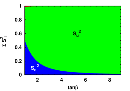
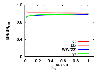
The loop diagrams needed for the reduced couplings to gluons $c_{gluon}$ and photons $c_{\gamma}$ are parametrized as effective couplings within NMSSMTools.Das:2011dg If the reduced couplings are SM-like, the Higgs mixing matrix elements are adjusted such that the reduced couplings are 1 as function of $\tan\beta$, which is possible if one chooses $S_{iu}\approx\sin\beta$ and $S_{id}\approx\cos\beta$, as is obvious from Eq. 4. In this case the couplings to gauge bosons take automatically SM-like values: $c_{W/Z}=\cos\beta\cdot S_{id}+\sin\beta\cdot S_{iu}\approx\cos^{2}\beta+\sin^{2}\beta\approx 1$. The components to the sum of the Higgs mixing matrix elements squared of the 125 GeV SM-like Higgs boson are shown in Fig. 1 as function of $\tan\beta$. One observes that $S_{u}$ is the dominant component in the linear combination of Eq. 1 for the SM-like Higgs boson for $\tan\beta>2$. In contrast, for the heavy Higgs $H_{3}$ the dominant component is the down-type component, as can be seen from the term $S_{3d}>0.97$ in Table 4 of Appendix C, which will be discussed later in detail. The square of the singlet component is hardly visible and represented by the thin (red) line at the top of the figure.

The couplings of the 125 GeV Higgs boson can be extracted from experimentally accessible observables such as cross sections times branching ratios (BRs). The cross section times BR relative to the SM values is also known as the signal strength $\mu$ and defined as:

$$\mu_{j}^{i}=\frac{\sigma_{i}\times BR_{j}}{(\sigma_{i}\times BR_{j})_{SM}}=c_{i}^{2}\cdot\frac{BR_{j}}{(BR_{j})_{SM}}.$$ (5)

So the signal strength is obtained by the production cross section $\sigma_{i}$ for mode $i$ times the corresponding BR for decay $j$, each normalized to the SM expectation. Normalized cross sections are called reduced cross sections, which are given by the square of the reduced couplings $c_{i}$. In the following we focus on the main Higgs boson production modes with the following reduced couplings $c_{i}$: the effective reduced gluon coupling $c_{gluon}$ for gluon fusion (ggf), $c_{W/Z}$ for vector boson fusion (VBF) and Higgs Strahlung (VH) and $c_{u}$ for top fusion (tth). We consider two fermion final states (b-quarks and $\tau$-leptons) and two boson final states ($W/Z$ and $\gamma\gamma$) for different production modes. VBF and VH share the same reduced couplings, so they can be combined to VBF/VH. This leads to 8 signal strengths in total, namely 4 fermionic and 4 bosonic signal strengths:

$$\mu_{\tau\tau}^{VBF/VH} \mu_{\tau\tau}^{ggf} \mu_{bb}^{VBF/VH} \mu_{bb}^{tth},$$ , , ,

$$\mu_{ZZ/WW}^{VBF/VH} \mu_{ZZ/WW}^{ggf} \mu_{\gamma\gamma}^{VBF/VH} \mu_{\gamma\gamma}^{ggf}.$$ , , , (6)

Figure 2: Sketch of the sampling technique to determine the allowed NMSSM parameter space. The sampling is done by performing a Minuit fit on each cell of the 3D Higgs mass space (left box) to determine the corresponding 7 free NMSSM parameters (right box). The relation between the NMSSM parameters and the Higgs masses is encoded in NMSSMTools. The second-lightest Higgs boson is chosen to be the 125 GeV Higgs boson, but we repeat the fit in case $m_{H1}$=125 GeV. Then the $m_{H1}$ becomes an $m_{H2}$ axis in the grid on the left. The 3D Higgs mass space can be restricted to the experimentally accessible Higgs masses and the low dimensionality allows a fit to each cell of the grid. This non-random sampling guarantees complete coverage of the corresponding 7D NMSSM parameter space.

III Analysis method

The scanning method is described in detail in Paper I.Beskidt:2019mos Here we shortly repeat the essential features in order to highlight differences, which are needed to allow for deviations from SM expectations. In Paper I no deviations from SM-like couplings were assumed in the fit. The semi-constrained NMSSMDjouadi:2008yj ; Ellwanger:2009dp has in total nine free parameters:

$${m_{0}},~{}{m_{1/2}},~{}A_{0},~{}\tan\beta,~{}\lambda,~{}\kappa,~{}A_{\lambda},~{}A_{\kappa},~{}\mu_{eff}.$$ (7)

Table 1: Differences of the fitting procedures from Paper I (middle column) and the one applied in this analysis (last column).

Procedure	standard (Paper I)	modified (this paper)
Input	$A_{1},H_{1/2},H_{3}$, $H_{1/2}=$125 GeV, $\mu_{no-loop}=$1	$A_{1},H_{1/2},H_{3}$, $H_{1/2}=$125 GeV, $\mu_{sel}=\mu_{theo}$
Output	$\tan\beta,A_{0},A_{\kappa},A_{\lambda},\mu_{eff},\lambda,\kappa$	$\tan\beta,A_{0},A_{\kappa},A_{\lambda},\mu_{eff},\lambda,\kappa$
$\chi^{2}$ constraints	$\chi^{2}_{H_{S}}$, $\chi^{2}_{H_{3}}$, $\chi^{2}_{A_{1}}$, $\chi^{2}_{H_{SM}}$, $\chi^{2}_{LEP}$, $\chi^{2}_{LHC}$ , $\chi^{2}_{\mu_{no-loop}}$	$\chi^{2}_{H_{S}}$, $\chi^{2}_{H_{3}}$, $\chi^{2}_{A_{1}}$, $\chi^{2}_{H_{SM}}$, $\chi^{2}_{LEP}$, $\chi^{2}_{LHC}$, $\chi^{2}_{\mu_{sel}}$

The latter six parameters in Eq. 7 enter the Higgs mixing matrix at tree level, see Appendix A, and thus form the 6D parameter space of the NMSSM Higgs sector. The coupling $\lambda$ represents the coupling between the Higgs singlet and doublets, while $\kappa$ determines the self-coupling of the singlet. $A_{\lambda}$ and $A_{\kappa}$ are the corresponding trilinear soft breaking terms. $\mu_{eff}$ represents an effective Higgs mixing parameter, which is related to the vev of the singlet $s$ via the coupling $\lambda$, i.e. $\mu_{eff}=\lambda\cdot s$. In addition, we have the GUT scale parameters of the constrained MSSM (CMSSM) ${m_{0}}$ and ${m_{1/2}}$ denoting the common mass scales of the spin 0 and spin 1/2 SUSY particles at the GUT scale. The trilinear coupling $A_{0}$ at the GUT scale is correlated with $A_{\lambda}$ and $A_{\kappa}$, so fixing it would restrict the range of $A_{\lambda}$ and $A_{\kappa}$ severely. Therefore, $A_{0}$ is considered a free parameter in the fit, which leads in total to 7 free parameters and thus a 7D NMSSM parameter space. For each set of the NMSSM parameters the 6 Higgs boson masses are completely determined. The masses of the heavy Higgs bosons $A_{2}$, $H_{3}$ and $H^{\pm}$ are approximately equal, so only one of the masses is independent. Furthermore, one of the masses has to be 125 GeV. Then only 3 Higgs masses are free, e.g. $m_{A_{1}}$, $m_{H_{1}}$ and $m_{H_{3}}$. Each set of parameters in the 7D NMSSM parameter space determines a mass combination in the 3D Higgs mass space and vice versa, each mass combination in the 3D mass space corresponds to given regions in the 7D parameter space. Hence it is advantageous to scan the lower dimensional Higgs mass space, especially since this space can be limited to mass ranges accessible to accelerators. Furthermore, the lower dimensionality allows to fit each mass combination in the grid of Fig. 2. Such a non-random scan guarantees a complete coverage of the corresponding 7D parameter region. A complete coverage is hardly reachable by a random scan in the 7D parameter space because of the high correlations between the parameters, as discussed in Paper I.

The transition of the 3D Higgs mass space to the corresponding 7D NMSSM parameter space can be obtained from a Minuit fit James:1975dr , as sketched in Fig. 2 and described in detail in Paper I. The theoretical connection between the NMSSM parameters and masses are obtained from NMSSMTools 5.2.0.Das:2011dg We included all available radiative correctionsoption , which is important, since the NMSSM radiative corrections to the Higgs boson can lower the mass by several GeV.Degrassi:2009yq The main contributions and free parameters for the standard fit procedures from Paper I have been summarized in Table 1 in the middle column.

The 4 signal strengths $\mu_{\tau\tau}^{VBF/VH}$, $\mu_{bb}^{VBF/VH}$, $\mu_{ZZ/WW}^{VBF/VH}$ and $\mu_{bb}^{tth}$ do not include loops in which non-SM particles could contribute. They are generically referred to as $\mu_{no-loop}$. The signal strengths from gluon fusion and/or decay into gammas include loop diagrams at lowest order, so the SUSY particles can contribute leading to deviations from the SM prediction. They are referred to as $\mu_{loop}$. In Paper I all $\mu_{no-loop}$ were required to be 1, but in this analysis we are looking for deviations from SM expectations, so we do not require $\mu_{no-loop}=1$. Deviations from SM expectations can have several physical origins, e.g. additional decays of the 125 GeV Higgs boson into lighter particles or modifications of the Higgs couplings via the Higgs mixing elements, which changes the Higgs content. These possibilities will be discussed in detail below.

Deviations were investigated by a modified fit requiring at least one signal strength to deviate from the SM prediction, i.e. $\mu\neq 1$, which can be enforced in the fit by replacing the $\chi^{2}_{\mu_{no-loop}}$ term in the bottom line of the middle column of Table 1 by a term $\chi^{2}_{\mu_{sel}}=(\mu_{sel}-\mu_{theo})^{2}/\sigma^{2}_{\mu}$, which forces $\mu_{sel}\approx\mu_{theo}$ for a minimal $\chi^{2}$ value. For the signal strength deviating from the SM expectation ($\mu_{sel}$) we usually select $\mu_{\tau\tau}^{VBF/VH}$, but other choices from the 8 signal strengths in Eq. 6 can be taken as well, which leads to similar results. The fit usually converges to a minimal $\chi^{2}$ value with $\mu_{theo}$ selecting the required deviation from the SM expectation. If the fit does not converge or does not reach a small $\chi^{2}$ value, this means the required deviations cannot be reached in the NMSSM or the selected parameter space does not fulfill all experimental constraints. Such mass combinations are rejected.

In comparison with the standard fit in the middle column of Table 1 one has 3 constraints less, since in the middle column $\chi^{2}_{\mu_{no-loop}}$ all four $\mu_{no-loop}$ values were required to be equal 1, while in this analysis the test statistic contribution $\chi^{2}_{\mu_{sel}}$ requires only $\mu_{sel}=\mu_{theo}$, as shown in the right column of Table 1. The reduction of the constraints still leads to converging fits. The reason is the high correlations between the parameters as demonstrated in Paper I. This reduces effectively the number of free parameters.

The fit is performed for each cell of the grid in Fig. 2, thus completely scanning the parameter space and checking where signal strength deviations of the size $\mu_{theo}$ are allowed taking into account the experimental constraints. From the fitted parameters in a fit with a single no-loop signal strength required to deviate from 1 the other signal strengths can be calculated and one can see, if they deviate in the same or in opposite directions in comparison to $\mu_{sel}$, which are called correlated or anti-correlated deviations, respectively.

IV Signal strength deviations of the 125 GeV Higgs boson from SM expectations

The signal strengths $\mu$ are given by the product of cross sections and BRs, see Eq. 5, so deviation from the SM expectation of $\mu=1$ can be obtained by deviations in cross sections or in branching ratios or in both. This leads to three different cases for deviations of the signal strengths of the 125 GeV Higgs boson from SM expectations:

• CASE I: Additional decays. The decay of the 125 GeV Higgs boson with SM couplings into particles with a mass $m<0.5m_{Higgs}$ leads to modifications of the total width, which changes all BRs in a correlated way. This leads to correlated deviations of the signal strengths.

• CASE II: Small Higgs mixing between the 125 GeV and the singlet Higgs boson. A modification of the Higgs mixing matrix elements leads to anti-correlated deviations because the total width stays almost constant. But the coupling to down-type fermions and hence the corresponding BRs decrease, which is largely compensated by an increase of the BRs to vector bosons, leading to anti-correlated BRs and thus anti-correlated fermionic and bosonic signal strengths.

• CASE III: Strong Higgs mixing between the 125 GeV and the singlet-like Higgs boson. A strong mixing and thus a large singlet component of the 125 GeV Higgs boson can be reached, if both masses are close to each other. This leads to correlated deviations of the signal strengths, because the singlet component of the 125 GeV Higgs boson does not couple to SM particles, so the reduced couplings decrease in a correlated way. Since a different Higgs mixing does not change the BRs significantly, a correlated decrease of the couplings leads to a correlated decrease of the signal strengths.

CASE Ia	CASE Ib	CASE Ic

Figure 3: BRs of the 125 GeV Higgs boson into lighter particles as function of the mass of the lighter particle, which can be neutralinos (CASE Ia), the light pseudo-scalar Higgs boson $A_{1}$ (CASE Ib) or the lightest Higgs boson $H_{1}$ (CASE Ic). The BRs are shown for $\mu_{sel}=\mu_{\tau\tau}^{VBF/VH}$ and $\mu_{theo}$=0.7 and 0.9. One observes that the BRs are directly related to the deviations of the signal strengths from the SM expectation, namely the BR is approximately $1-\mu_{theo}$ (see text).

	$\mu_{sel}=\mu_{\tau\tau}^{VBF/VH}\approx\mu_{theo}=0.9$	$\mu_{sel}=\mu_{\tau\tau}^{VBF/VH}\approx\mu_{theo}=0.7$
ggf
VBF/VH

Figure 4: Fitted signal strengths $\mu$ as function of the singlet-like Higgs mass for different values of $\mu_{sel}$, different production cross sections and different final states. The left(right) panels show results for $\mu_{theo}$ 0.9(0.7), while the top and bottom rows correspond to the ggf and VBF/VH production modes, respectively. The regions with $m_{H_{S}}<60$ GeV correspond to CASE I and is a combination of CASEs Ia, Ib and Ic in Fig. 3. The region with $m_{H_{S}}>60$ GeV correspond to CASE II, while the narrow stripe for $m_{H_{S}}\sim 125$ GeV corresponds to CASE III. One observes correlated signal strengths for bosons and fermions in CASE I, i.e. they deviate from 1 by the same amount, while for CASE II an anti-correlation of the bosonic and fermionic signal strengths is observed, i.e. the deviations from 1 go in opposite directions.

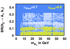
For CASE I deviations are obtained by decays into light neutralinos (CASE Ia), light pseudo-scalar Higgs bosons (CASE Ib) and light singlet-like Higgs bosons (CASE Ic). The BRs are shown in Fig. 3 for each case as function of the mass of the final state particles for two values of $\mu_{theo}$, namely 0.7 and 0.9, respectively. Here $\mu_{sel}=\mu_{\tau\tau}^{VBF/VH}$ was chosen, but similar results are found for other choices of $\mu_{sel}$. The Higgs mass space is scanned on the grid in Fig. 2 in 1 GeV steps. The neutralino mass is calculated from the fitted NMSSM parameters for each cell in the 3D Higgs mass space. The fit usually converges with a good $\chi^{2}$ value meaning that the mass combination is theoretically allowed and fulfills all experimental constraints. Additional decays into light particles increase the total width $\Gamma_{tot}$ of the 125 GeV Higgs boson: $\Gamma_{tot}^{*}=\Gamma_{tot}+\Gamma_{light}>\Gamma_{tot}$. This leads to a reduction of the BRs of the 125 GeV SM-like Higgs boson, where it is convenient to normalize to the BR of the SM. Using the BR into $\tau$ leptons as an example one can write: ${BR_{\tau\tau}^{*}}/{BR_{\tau\tau,SM}}={\Gamma_{tot}}/{(\Gamma_{tot}+\Gamma_{light})}\approx 1-\Gamma_{light}/\Gamma_{tot}\approx 1-BR_{light}$. So for CASE I one basically always finds the deviations from the SM signal strength to be determined by the BR into light particles, i.e. one finds $\mu\approx 1-BR_{light}$. This relation approximately holds for the various light particles in the different panels of Fig. 3. Sometimes it happens that several particles are simultaneously light, since the masses are correlated, which can be seen already from the approximate expressions $m_{A_{1}}\sim\lambda\mu_{eff}$ and $m_{\tilde{\chi}_{0}^{1}}\sim 2\kappa/\lambda\mu_{eff}$ in Appendix A or that the mixing between $H_{1}$ and $H_{2}$ (CASE II) changes simultaneously with the total width (CASE I). This leads to the broadening of the bands in Fig. 3, where we summed over all mass combinations of the grid in Fig. 2.

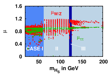
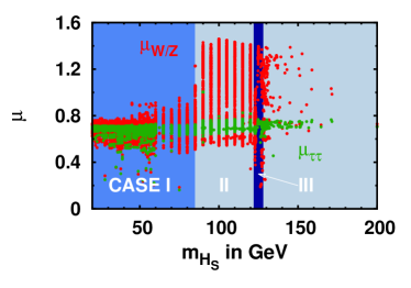
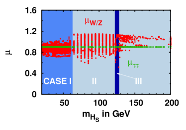
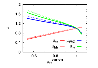
To study the CASEs II and III, where the deviations of the signal strengths are caused by the Higgs mixing with the singlet, we concentrate on the signal strength as function of the mass of the singlet-like Higgs boson $m_{H_{S}}$. We select again $\mu_{sel}=\mu_{\tau\tau}^{VBF/VH}$ and $\mu_{theo}=0.9$ or $0.7$. Fig. 4 shows the fermionic and bosonic signal strengths as function of $m_{H_{S}}$ for two production channels: ggf (top row in Fig. 4) and VBF/VH (bottom row in Fig. 4). One observes the following features: for $m_{H_{S}}<60$ GeV in the top left panel $\mu_{W/Z}$ and $\mu_{\tau\tau}$ are both equal to $\mu_{sel}=0.9\approx 1-BR_{light}$, as expected for CASE I. For $m_{H_{S}}>60$ GeV the decays into fermions and bosons are anti-correlated, as expected for CASE II: Since the sum of the partial widths (= total width) stays constant, a change of one partial width has to be compensated by an opposite change in one or more other partial widths (or BRs). Indeed, one observes the signal strengths for $\mu_{W/Z}$ to be above the ones for $\mu_{\tau\tau}$. The effect becomes more pronounced, if one requires larger deviations, e.g. $\mu_{theo}=0.7$, which is shown on the right side of Fig. 4. Note that the spread is large because the results are shown for all mass combinations in the grid of the Higgs mass space and for different stop masses (determined by different values of ${m_{0}},{m_{1/2}}$). All cases will be discussed in more detail in the next section, where we do not average over all mass combinations, but consider for each case a representative mass combination, which better shows the salient features.

(a)	(b)
(c)	(d)

Figure 5: The figure demonstrates in the top left panel (a) the correlated deviation of all signal strengths from the SM expectation 1 as function of $\mu_{\tau\tau}^{VBF/VH}$ by the overlapping lines. $\mu_{\tau\tau}^{VBF/VH}$ was required to deviate from the SM expectation by fitting it to a value $\mu_{theo}<1$ for a specific mass combination characterized by allowed decays into neutralinos (CASE I). The deviations can either come from deviations of the couplings or from the BRs. Here it is clearly caused by the BRs, since all reduced couplings correspond to the SM expectation of 1, as demonstrated in panels (b) and (c). The allowed neutralino decays increase the invisible width (line with negative slope in panel (d)), which increase the total width and hence reduces the BRs for all other channels in the same way (overlapping lines with positive slope in panel (d)). This leads to the same (=correlated) change in all signal strengths (overlapping lines with positive slope in panel (a)) given the constant couplings in panels (b) and (c), which is true for all production modes, as demonstrated by the overlap of the solid and dashed lines in (a) representing the signal strengths for the VBF/VH and ggf production mode, respectively.

(a)	(b)
(c)	(d)

Figure 6: As Fig. 5, but for CASE II. In this case the change in signal strengths in panel (a) originates from the change in reduced couplings, shown in panels (b) and (c). The variation of the signal strengths is obtained in the fit by varying predominatly the coupling to down-type fermions $c_{d}$ (lowest line in panel (b)), which varies predominantly the corresponding BRs (lowest line in panel (d)). The decrease of the BR to down-type fermions can be compensated by an increase in the bosonic BRs, since the sum of all BRs stays almost constant, if the total width stays almost constant. The anti-correlation in BRs leads to anti-correlations in the signal strengths, as shown in panel (a) by the lines with negative (positive) slopes for bosonic (fermionic) signal strengths.

(a)	(b)
(c)	(d)

Figure 7: As Fig. 5, but for CASE III. The variation of the signal strengths originates from a variation of all reduced couplings simultaneously (see (b) and (c)), while the BRs stay close to 1 (see (d)). The simultaneous variation of all reduced couplings is caused by the increase of the singlet component $S_{2s}$ of the 125 GeV Higgs boson. In this case all signal strengths change in a correlated way (see overlapping lines in (a)).

V Examples of signal strength deviations of the 125 GeV Higgs bosons from the SM expectations

V.1 CASE I: Deviations by decays of the 125 GeV Higgs boson into non-SM light particles

For CASE I either $m_{\tilde{\chi}_{1}^{0}}$ and/or $m_{A_{1}}$ and/or $m_{H_{1}}$ had to be smaller than about 60 GeV to allow decays of the 125 GeV Higgs boson into pairs of these light particles, which leads to deviations from the SM expectation. Here we investigate the deviations from the SM for a specific mass combination in the grid of Fig. 2 characterized by allowed decays into neutralinos (CASE Ia), in this case $m_{H1}=90~{}\mathrm{GeV},m_{H3}=2000~{}\mathrm{GeV}$ and $m_{A1}=200~{}\mathrm{GeV}$. As before, the signal strength $\mu_{\tau\tau}^{VBF/VH}$ is required to deviate from the SM expectation by fitting it to a value $\mu_{theo}\neq 1$. This is accomplished in the fit by increasing the invisible BR via the decrease of the neutralino mass, which can be changed in the fit to a specific value by adjusting the free parameters $\mu_{eff}$, $\lambda$ and $\kappa$ ($m_{\tilde{\chi}_{0}^{1}}\sim 2\frac{\kappa}{\lambda}\mu_{eff}$). This can be observed from the NMSSMTools output in Appendix C in Tables 2-7 for two examples, called P1 and P2, for $\mu_{theo}=1$ and 0.7, respectively. For CASE Ib ($m_{A_{1}}<60$ GeV) and CASE Ic ($m_{H_{1}}<60$ GeV) one cannot study the deviations for a fixed mass combination, since they require changes in $m_{A_{1}}$ and/or $m_{H_{1}}$, which contradicts the study for a fixed mass combination.

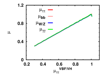
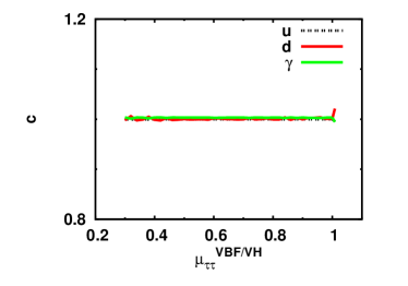
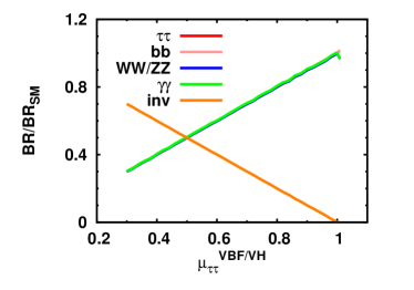
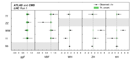
In the top left panel of Fig. 5 the signal strengths are shown for all 8 signal strengths as function of $\mu_{sel}=\mu_{\tau\tau}^{VBF/VH}$ between 0.3 and 1 by the overlapping solid (dashed) lines for the VBF/VH (ggf) production mode. Note that for the $b\bar{b}$ final states the ttH production mode is selected instead of ggf, as indicated in Eq. 6 before. Below $\mu_{theo}=0.3$ no good fit can be obtained. All signal strengths vary in a correlated way, as expected for CASE I. Since the signal strengths are the product of couplings squared and BRs relative to the SM values, we check which one is varying. Fig. 5(b) shows the reduced coupling $c$ as function of the selected signal strength $\mu_{\tau\tau}^{VBF/VH}$ for $c_{u}$, $c_{d}$ and $c_{\gamma}$, which are all close to 1. The same is true for $c_{W/Z}$ and $c_{gluon}$ in Fig. 5(c). However, from Fig. 5(d) one observes that the correlated change in the signal strengths in Fig. 5(a) originates from the correlated change of BRs into visible final states (overlapping lines with a positive slope), which are anti-correlated with the invisible BR (line with negative slope). For $\mu_{\tau\tau}^{VBF/VH}=1$ the invisible BR is zero, while all other reduced BRs are equal 1, so no deviations from the SM expectations are observed. Note that experimentally the signal strengths are constrained by the data, but they are not yet precise, as shown in Fig. 8 of Appendix B for the data from the ATLAS and CMS experiments, which were combined by the Particle Data Group.Tanabashi:2018oca

V.2 CASE II: Deviations by Higgs mixing

For CASE II a mass combination with all particles above 60 GeV is selected, so no decays into light particles can occur, in this case the mass combination $m_{H1}=90~{}\mathrm{GeV},m_{H3}=1000~{}\mathrm{GeV}$ and $m_{A1}=200~{}\mathrm{GeV}$ was selected. As before, regions with deviations from the SM expectations are searched for by looking for a good $\chi^{2}$ value under the constraint $\mu_{sel}=\mu_{\tau\tau}^{VBF/VH}=\mu_{theo}<1$. The fit accomplishes this by modifying the NMSSM parameters leading to deviations in the Higgs mixing, as shown in Appendix C in Table 2 for two selected mass combinations, P3 and P4, for $\mu_{theo}=1$ and 0.7, respectively. The change in mixing can be observed e.g. by the change in $S_{2s}$ in Table 4 for P4 in comparison with P3.

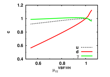
By fitting the down-type signal strength $\mu_{\tau\tau}^{VBF/VH}$ to $\mu_{theo}<1$, the reduced coupling $c_{d}$ decreases, as shown in Fig. 6(b) (lowest line), while all other reduced couplings, shown in Fig. 6(b) and 6(c), vary less by the variation of the mixing. The reduction in $c_{d}$ with much flatter dependencies for $c_{u}$ and $c_{W/Z}$ can be easily derived from Eq. 4 for larger values of $\tan\beta$. For the reduced couplings $c_{gluon}$ and $c_{\gamma}$ additional deviations from 1 can be caused by SUSY contributions in the loops. These are small in this case, where the lightest stop mass is about 1.2 TeV, as shown in Table 3 of Appendix C. The decrease in $c_{d}$ leads to decreasing BRs into down-type fermion final states, which are displayed in Fig. 6(d) as function of $\mu_{\tau\tau}^{VBF/VH}$ (overlapping lines with a positive slope). The total width stays almost constant, if no new decay modes open up, so the sum of the BRs stays almost constant, implying a decrease of the fermionic BRs must be compensated by a larger BR for bosonic final states (lines with negative slopes in panel (d)), leading to an anti-correlation of the corresponding signal strengths, as demonstrated in Fig. 6(a): The fermionic signal strengths $\mu_{\tau\tau},\mu_{bb}$ (lines with positive slopes) follow $\mu_{sel}$, while the bosonic signal strengths $\mu_{W/Z},\mu_{\gamma\gamma}$ (lines with negative slopes) increase with decreasing $\mu_{\tau\tau}^{VBF/VH}$. The anti-correlations in signal strengths and BRs is demonstrated numerically by comparing e.g. the signal strengths (BRs) for $H_{2}\rightarrow bb$ and $H_{2}\rightarrow ZZ/WW$ in Tables 6 and 7 of Appendix C for P4. This anti-correlation is in contrast to CASE I, shown in Fig. 5, where all signal strengths decrease and follow approximately $\mu_{\tau\tau}^{VBF/VH}$. In addition, the reduced couplings, especially $c_{d}$, vary significantly, while for CASE I the reduced couplings equal 1 as function of $\mu_{\tau\tau}^{VBF/VH}$.

V.3 CASE III: Deviations by strong mixing with the singlet

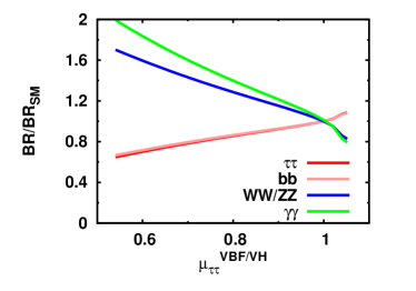
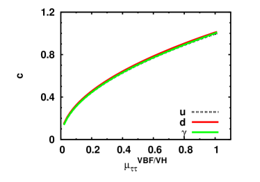
In CASE III we select $m_{H1}=122~{}\mathrm{GeV},m_{H3}=1300~{}\mathrm{GeV},m_{A1}=200~{}\mathrm{GeV}$, so $H_{1}$ is close in mass to $H_{2}$ (125 GeV), which can lead to a stronger mixing between $H_{1}$ and $H_{2}$ than in CASE II. As for the previous cases, we force $\mu_{\tau\tau}^{VBF/VH}$ to deviate from 1 by requiring $\mu_{sel}=\mu_{\tau\tau}^{VBF/VH}=\mu_{theo}<1$. The required deviation in the fit is accomplished by increasing the mixing between $H_{1}$ and $H_{2}$, as demonstrated in Table 4 of Appendix C for the selected mass combinations, P5 and P6, for $\mu_{theo}=1$ and 0.7, respectively. One observes that the singlet component $H_{2s}$ of the 125 GeV Higgs boson becomes 0.56 for P6, while it is 0.008 for P5. The singlet component does not couple to SM particles, so the couplings to all fermions and bosons decrease from 1 for P5 to 0.83 for P6 with $\mu_{\tau\tau}^{VBF/VH}=0.7$, as shown in Table 5 of Appendix C in the $H_{2}$ block. The dependencies of the reduced couplings on $\mu_{\tau\tau}^{VBF/VH}$ are displayed in Figs. 7(b) and 7(c). In contrast to CASE I (Fig. 5) and CASE II (Fig. 6) the BRs of the 125 GeV Higgs boson stay close to the SM expectation of 1 as function of $\mu_{\tau\tau}^{VBF/VH}$, as shown in Fig. 7(d). The constant BRs and decreasing couplings lead to correlated deviations for the signal strengths, as shown in Fig. 7(a) for fermionic and bosonic final states.

VI Conclusion

Examples for signal strengths deviating from the SM expectation are presented and the correlations between the signal strengths for fermionic and bosonic final states have been determined. We find three different cases to obtain signal strengths deviating from the SM prediction, i.e. deviating from 1. For the first case, additional decays of the 125 GeV Higgs boson with SM couplings into particles with $m<0.5m_{Higgs}$ are possible (CASE I). This leads to a modification of the total width, which changes all BRs in a correlated way, and hence leads to correlated deviations of the signal strengths, as summarized in Fig. 5. In the second case, a modification of the Higgs mixing changes preferentially the reduced couplings to down-type fermions and thus the corresponding BRs (CASE II). The total width stays almost constant by a modification of the Higgs mixing, so the sum of the BRs stays constant. Hence the decrease of BRs into fermionic final states has to be compensated by an increase of BRs into bosonic final states. This leads to anti-correlated deviations of the fermionic and bosonic signal strengths for CASE II, as summarized in Fig. 6. In the third case the singlet-like and SM-like Higgs bosons are rather close in mass, which allows for a strong mixing. In this case the fit leads to a significant enhancement of the singlet component of the 125 GeV Higgs boson (CASE III), which reduces the couplings to SM particles for all final states and thus leads to correlated deviations of fermionic and bosonic signal strengths, as summarized in Fig. 7. The three different cases can be related to the corresponding regions in the Higgs mass space, as shown by the projections onto the $m_{A_{1}}$ and $m_{H_{S}}$ axes in Figs. 3 and 4. These projections are largely independent of the third mass $m_{H_{3}}$ in the Higgs mass space in Fig. 2.

Allowed upper limits on the possible deviations of the signal strengths are proportional to the measured upper limits for the deviations from the SM predictions, which are presently still large. Precision measurements at a linear collider would allow to search for deviations of the 125 GeV Higgs boson signal strengths with much higher precision. This would allow to study correlations of possible deviations in much more detail and either strongly constrain the NMSSM parameter space or point to preferred regions of mass space in case correlated or anti-correlated deviations between fermionic and bosonic signal strengths from SM expectations are found.

Appendix A Higgs and neutralino mixing matrix in the NMSSM

The neutral components from the two Higgs doublets and singlet mix to form three physical CP-even scalar ($S$) bosons and two physical CP-odd pseudo-scalar ($P$) bosons. The elements of the corresponding mass matrices at tree level read:Miller:2003ay

$${\cal M}^{2}_{S,11} = M_{A}^{2}+(M_{Z}^{2}-\lambda^{2}v^{2})\sin^{2}2\beta,$$

$${\cal M}^{2}_{S,12} = -\frac{1}{2}(M_{Z}^{2}-\lambda^{2}v^{2})\sin 4\beta,$$

$${\cal M}^{2}_{S,13} = -\frac{1}{2}(M_{A}^{2}\sin 2\beta+\frac{2\kappa\mu^{2}}{\lambda})\frac{\lambda v}{\mu}\cos 2\beta,$$

$${\cal M}^{2}_{S,22} = M_{Z}^{2}\cos^{2}2\beta+\lambda^{2}v^{2}\sin^{2}2\beta,$$ (8)

$${\cal M}^{2}_{S,23} = 2\lambda\mu v\left[1-(\frac{M_{A}\sin 2\beta}{2\mu})^{2}-\frac{\kappa}{2\lambda}\sin 2\beta\right],$$

$${\cal M}^{2}_{S,33} = \frac{1}{4}\lambda^{2}v^{2}(\frac{M_{A}\sin 2\beta}{\mu})^{2}+\frac{\kappa\mu}{\lambda}(A_{\kappa}+\frac{4\kappa\mu}{\lambda})-\frac{1}{2}\lambda\kappa v^{2}\sin 2\beta,$$

$${\cal M}^{2}_{P,11} = \frac{\mu(\sqrt{2}A_{\lambda}+\kappa\frac{\mu}{\lambda})}{\sin 2\beta}=M^{2}_{A},$$

$${\cal M}^{2}_{P,12} = \frac{1}{\sqrt{2}}\left(M^{2}_{A}\sin 2\beta-3\frac{\kappa}{\lambda}\mu^{2}\right)\frac{v\lambda}{\mu},$$ (9)

$${\cal M}^{2}_{P,22} = \frac{1}{2}\left(M^{2}_{A}\sin 2\beta+3\frac{\kappa}{\lambda}\mu^{2}\right)\frac{v^{2}}{\mu^{2}}\lambda^{2}\sin 2\beta-\frac{3}{\sqrt{2}\frac{\kappa}{\lambda}\mu A_{\kappa}}.$$

One observes that the element ${\cal M}^{2}_{S,22}$, which corresponds to the tree-level term of the lightest MSSM Higgs boson, can be above $M^{2}_{Z}$ because of the $\lambda^{2}v^{2}\sin^{2}2\beta$ term. The diagonal element ${\cal M}^{2}_{P,11}$ at tree level corresponds to the pseudo-scalar Higgs boson in the MSSM limit of small $\lambda$, so it is called $M_{A}$.

Within the NMSSM the singlino, the superpartner of the Higgs singlet, mixes with the gauginos and Higgsinos, leading to an additional fifth neutralino. The resulting mixing matrix reads:Ellwanger:2009dp ; Staub:2010ty

$${\cal M}_{0}=\left(\begin{array}[]{ccccc}M_{1}&0&-\frac{g_{1}v_{d}}{\sqrt{2}}&\frac{g_{1}v_{u}}{\sqrt{2}}&0\\ 0&M_{2}&\frac{g_{2}v_{d}}{\sqrt{2}}&-\frac{g_{2}v_{u}}{\sqrt{2}}&0\\ -\frac{g_{1}v_{d}}{\sqrt{2}}&\frac{g_{2}v_{d}}{\sqrt{2}}&0&-\mu_{\mathrm{eff}}&-\lambda v_{u}\\ \frac{g_{1}v_{u}}{\sqrt{2}}&-\frac{g_{2}v_{u}}{\sqrt{2}}&-\mu_{\mathrm{eff}}&0&-\lambda v_{d}\\ 0&0&-\lambda v_{u}&-\lambda v_{d}&2\kappa s\end{array}\right)$$ (10)

with the gaugino masses $M_{1}$, $M_{2}$, the gauge couplings $g_{1}$, $g_{2}$ and the Higgs mixing parameter $\mu_{eff}$ as parameters. Furthermore, the vacuum expectation values of the two Higgs doublets $v_{d}$,$v_{u}$, the singlet $s$ and the Higgs couplings $\lambda$ and $\kappa$ enter the neutralino mass matrix.

The upper left $4\times 4$ submatrix of the neutralino mixing matrix corresponds to the MSSM neutralino mass matrix, see e.g. Ref. Martin:1997ns .

The neutralino mass eigenstates are obtained from the diagonalization of ${\cal M}_{0}$ in Eq. 10 and are linear combinations of the gaugino and Higgsino states:

$$\footnotesize{\tilde{\chi}^{0}_{i}={\cal N}(i,1)\left|\tilde{B}\right\rangle+{\cal N}(i,2)\left|\tilde{W}^{0}\right\rangle+{\cal N}(i,3)\left|\tilde{H}^{0}_{u}\right\rangle+{\cal N}(i,4)\left|\tilde{H}^{0}_{d}\right\rangle+{\cal N}(i,5)\left|\tilde{S}\right\rangle.}$$ (11)

Typically, the diagonal elements in Eq. 10 dominate over the off-diagonal terms, so the neutralino masses are of the order of $M_{1}$, $M_{2}$, while the heavier Higgsinos are of the order of the mixing parameter $\mu_{eff}$ and ithe the lightes (singlino-like) neutralino is of the order of $2\kappa s\ =\ 2(\kappa/\lambda)\mu_{eff}$.

Appendix B Experimental data on the signal strengths of the 125 GeV Higgs boson

All LHC measurements have been combined by the Particle Data Group to obtain the most precise results.Tanabashi:2018oca A Summary of the combinations is shown in Fig. 8.

Figure 8: Combined measurements of the products $\sigma\cdot$ BR for the five main production and five main decay modes. The hatched combinations require more data for a meaningful confidence interval to be provided. The figure is taken from Tanabashi:2018oca .

Appendix C Output of NMSSMTools for six representative mass combinations P1 to P6

In Sect. V examples of mass combinations for the three possible cases for deviations of the signal strengths of the 125 GeV Higgs boson from the SM-expectation were discussed. To see which parameters need changes for deviations from the SM-expectation we present for each example the parameters without (with) deviation, i.e. $\mu_{theo}=1$($\mu_{theo}=0.7$). For CASE I we select the mass combinations $P_{1}$ and $P_{2}$, where the last point corresponds to the deviations presented in Fig. 5. Similarly, we select $P_{3}$ and $P_{4}$ for CASE II, where $P_{4}$ corresponds to the deviations presented in Fig. 6 and $P_{5}$ and $P_{6})$ for CASE III with the deviations presented in Fig. 7. The fitted NMSSM parameters for the representative mass combinations for $H_{1},H_{3},A_{1}$ from Figs. 5-7 are listed in Table 2. From these fitted parameters NMSSMTools calculates all masses (shown in Table 3) and the Higgs and neutralino mixing matrices (shown in Table 4). The reduced couplings are listed in Table 5. The signal strengths and BRs are shown in 6 and 7, respectively. All values are obtained from the output of NMSSMTools.

Table 2: List of fitted NMSSM parameters for representative mass combinations P1 to P6.

P	1	2	3	4	5	6
$\mu_{\tau\tau}^{VBF/VH}$	1	0.7	1	0.7	1	0.7
$\tan\beta$	4.12	3.96	5.36	6.57	12.87	19.47
$A_{0}$ in GeV	-654.85	-553.88	-617.09	520.12	-2467.63	-2295.48
$A_{\kappa}$ in GeV	3779.52	3724.97	4673.16	4444.88	-156.54	-156.55
$A_{\lambda}$ in GeV	4325.18	4415.52	3300.37	3553.43	319.80	-126.42
$\lambda\cdot 10^{-1}$	6.31	6.31	6.97	6.50	0.04	0.04
$\kappa\cdot 10^{-1}$	0.37	0.28	2.51	3.20	0.03	0.04
$\mu_{eff}$ in GeV	459.38	475.24	184.48	146.19	103.64	104.11

Table 3: Masses of Higgs bosons, sparticles and gauginos in GeV for the representative mass combinations P1 to P6. The values of $H_{1},H_{3}$ and $A_{1}$ represent the chosen mass combination in the grid of Fig. 2. One observes the approximate mass degeneracy of the heavy Higgs masses ($H_{3},A_{2}$ and $H^{\pm}$). $H_{2}$ is the observed 125 GeV Higgs mass and $H_{1}$ the singlet-like boson (see large value of $S_{1s}$ in Table 4). ).

P	1	2	3	4	5	6
$\mu_{\tau\tau}^{VBF/VH}$	1	0.7	1	0.7	1	0.7
$H_{1}$	90.0	90.0	90.0	90.0	122.9	122.9
$H_{2}$	125.2	125.2	125.2	125.2	125.2	125.3
$H_{3}$	2000.0	2000.0	1000.0	1000.0	1300.8	1300.0
$A_{1}$	200.0	200.0	200.0	200.0	200.0	200.0
$A_{2}$	2000.5	2000.6	998.1	997.7	1300.7	1300.0
$H^{\pm}$	1996.5	1996.6	990.1	990.7	1303.4	1302.7
$\tilde{d}_{L}$	2214.6	2214.3	2211.4	2209.9	2217.3	2218.3
$\tilde{d}_{R}$	2137.3	2137.0	2128.1	2128.6	2134.1	2136.6
$\tilde{u}_{L}$	2213.4	2213.1	2210.2	2208.6	2216.0	2217.0
$\tilde{u}_{R}$	2165.3	2165.0	2184.8	2173.3	2187.0	2180.8
$\tilde{s}_{L}$	2214.6	2214.3	2211.4	2209.9	2217.3	2218.3
$\tilde{s}_{R}$	2137.3	2137.0	2128.1	2128.6	2134.1	2136.6
$\tilde{c}_{L}$	2213.4	2213.1	2210.2	2208.6	2216.0	2217.0
$\tilde{c}_{R}$	2165.3	2165.0	2184.8	2173.3	2187.0	2180.7
$\tilde{b}_{1}$	1773.2	1777.3	1796.2	1884.5	1706.0	1701.9
$\tilde{b}_{2}$	2131.4	2131.6	2121.0	2122.2	2083.7	2030.4
$\tilde{t}_{1}$	1064.3	1078.1	1189.0	1427.4	950.8	1034.0
$\tilde{t}_{2}$	1792.4	1796.3	1814.5	1899.8	1731.7	1728.3
$\tilde{e}_{L}$	1206.3	1206.2	1233.7	1222.9	1232.0	1224.2
$\tilde{e}_{R}$	1021.0	1021.2	959.2	986.2	968.0	987.5
$\tilde{\nu}^{e}_{L}$	1204.1	1204.0	1231.5	1220.6	1229.6	1221.7
$\tilde{\mu}_{L}$	1206.3	1206.2	1233.7	1222.9	1232.0	1224.2
$\tilde{\mu}_{R}$	1021.0	1021.2	959.2	986.2	968.0	987.5
$\tilde{\nu}^{\mu}_{L}$	1204.1	1204.0	1231.5	1220.6	1229.6	1221.7
$\tilde{\tau}_{1}$	1016.1	1016.7	953.5	981.0	910.0	860.9
$\tilde{\tau}_{2}$	1204.3	1204.3	1231.5	1220.8	1209.9	1176.0
$\tilde{\nu}^{\tau}_{L}$	1202.1	1202.1	1229.2	1218.5	1207.4	1173.3
$\tilde{g}$	2237.4	2237.3	2239.2	2240.0	2240.3	2239.3
$\tilde{\chi}^{0}_{1}$	62.5	52.1	103.2	88.8	98.1	99.0
$\tilde{\chi}^{0}_{2}$	407.2	410.7	-220.3	-179.5	-110.9	-111.6
$\tilde{\chi}^{0}_{3}$	483.9	494.7	238.2	224.7	174.8	174.8
$\tilde{\chi}^{0}_{4}$	-483.9	-499.8	433.6	431.2	431.8	431.7
$\tilde{\chi}^{0}_{5}$	831.1	831.8	823.1	820.0	824.2	824.3
$\tilde{\chi}^{\pm}_{1}$	454.0	469.2	183.8	146.2	104.1	105.0
$\tilde{\chi}^{\pm}_{2}$	831.0	831.6	823.1	820.0	824.2	824.2

Table 4: Higgs mixing matrix elements in % for the scalar Higgs bosons $S_{ij}$ with $i=1,2,3$ and $j=d,u,s$. The Higgs mixing matrix elements for the pseudo-scalar Higgs bosons are labeled as $P_{ij}$ with $i=1,2$ and $j=d,u,s$ while the neutralino mixing matrix elements are denoted by $N_{ij}$ with $i=1,...,5$ and $j=1,...,5$. The components are defined in Eq. 11. One observes that for the mass combinations P1, P3 and P5 the 125 GeV Higgs boson has a large $S_{2u}$ component and a small singlet $S_{2s}$ component. The singlet component $S_{2s}$ increases in CASE II and CASE III with deviations from the SM-like signal strengths (mass combinations P4 and P6 with $\mu_{\tau\tau}^{VBF/VH}$=0.7). For CASE I the lightest neutralino (the dark matter candidate) is singlino-like with $N_{15}$=0.97, while for the other cases with larger mixing (P3 to P6) the singlino component $N_{15}$ decreases and the Higgsino components $N_{13}$ and $N_{14}$ increase.

P	1	2	3	4	5	6
$\mu_{\tau\tau}^{VBF/VH}$	1	0.7	1	0.7	1	0.7
$S_{1d}$	4.64	4.83	11.41	15.83	0.12	-2.86
$S_{1u}$	-1.60	-0.59	-2.54	30.50	0.83	-55.51
$S_{1s}$	99.88	99.88	99.31	93.91	99.99	83.13
$S_{2d}$	23.62	24.48	18.42	10.52	7.86	4.34
$S_{2u}$	97.17	96.96	98.29	94.05	99.69	83.02
$S_{2s}$	0.46	-0.62	0.40	-32.32	-0.83	55.58
$S_{3d}$	97.06	96.84	97.62	98.18	99.69	99.86
$S_{3u}$	-23.57	-24.48	-18.24	-15.00	-7.86	-5.20
$S_{3s}$	-4.88	-4.83	-11.69	-11.68	-0.05	-0.04
$P_{1d}$	-5.08	-5.13	-9.43	-9.13	-0.05	-0.03
$P_{1u}$	-1.23	-1.29	-1.76	-1.39	$<$ -0.01	$<$ -0.01
$P_{1s}$	99.86	99.86	99.54	99.57	99.99	99.99
$P_{2d}$	97.04	96.81	97.85	98.44	99.70	99.87
$P_{2u}$	23.56	24.46	18.26	14.98	7.75	5.13
$P_{2s}$	5.23	5.29	9.59	9.24	0.05	0.03
$N_{11}$	2.48	2.30	8.90	9.48	9.55	9.34
$N_{12}$	-2.26	-2.12	-7.61	-8.27	-8.19	-8.00
$N_{13}$	-1.83	-2.59	31.09	41.22	72.51	72.53
$N_{14}$	-22.24	-21.45	-62.58	-68.91	-67.70	-67.73
$N_{15}$	97.42	97.59	70.57	58.26	0.66	0.68
$N_{21}$	83.62	87.64	-3.39	-3.78	-5.32	-5.47
$N_{22}$	-8.55	-7.61	3.98	4.32	5.78	5.94
$N_{23}$	40.14	35.43	70.42	70.86	68.76	68.74
$N_{24}$	-35.08	-30.67	65.19	64.68	72.18	72.17
$N_{25}$	-9.58	-8.03	27.64	27.60	0.19	0.19
$N_{31}$	-54.69	47.99	11.46	-7.93	-0.06	-0.06
$N_{32}$	-16.71	18.17	-7.06	5.09	0.04	0.05
$N_{33}$	57.86	-60.72	63.23	-56.87	-0.61	-0.63
$N_{34}$	-57.11	59.69	-39.62	28.89	0.30	0.32
$N_{35}$	-10.95	10.77	-65.20	76.43	99.99	99.99
$N_{41}$	-2.38	-2.31	98.88	99.15	99.39	99.41
$N_{42}$	3.13	3.05	2.86	2.53	2.19	2.17
$N_{43}$	70.10	70.09	-7.66	-5.74	-3.26	-3.02
$N_{44}$	69.09	69.12	12.34	11.24	10.26	10.23
$N_{45}$	17.23	17.18	2.15	1.59	$<$ 0.01	$<$ 0.01
$N_{51}$	-1.89	-1.97	-1.22	-1.19	-1.10	-1.09
$N_{52}$	98.15	97.97	99.34	99.40	99.47	99.48
$N_{53}$	11.07	11.78	4.27	3.41	2.05	1.79
$N_{54}$	-15.50	-16.07	-10.57	-10.32	-9.99	-9.98
$N_{55}$	-1.01	-1.04	-0.40	-0.31	$<$ -0.01	$<$ 0.01

Table 5: The reduced couplings for all Higgs bosons to up-type fermions $c_{u}$, down-type fermions $c_{d}$, b-quarks $c_{b}$, W/Z-bosons $c_{W/Z}$, gluons $c_{gluon}$ and photons $c_{\gamma}$. One observes that for CASE I, represented by P1 and P2, the reduced couplings of $H_{2}$ are close to 1, even if the signal strength $\mu_{\tau\tau}^{VBF/VH}$=0.7. The deviations from the SM-like signal strength in P2 is caused by the change in BRs to neutralinos, as can be seen from the last row in Table 7. For the other cases the signal strength changes by a change of the reduced couplings, see columns for P4 and P6 in the $H_{2}$ block.

P		1	2	3	4	5	6
$\mu_{\tau\tau}^{VBF/VH}$		1	0.7	1	0.7	1	0.7
$H_{1}$	$c_{u}$	-0.017	-0.006	-0.026	0.308	0.008	-0.556
	$c_{d}$	0.196	0.197	0.622	1.052	0.016	-0.557
	$c_{b}$	0.196	0.196	0.622	1.050	0.016	-0.557
	$c_{W,Z}$	-0.004	0.325	-0.005	0.006	0.008	-0.556
	$c_{gluon}$	0.046	0.038	0.126	0.291	0.008	0.553
	$c_{\gamma}$	0.053	0.041	0.139	0.177	0.007	0.560
$H_{2}$	$c_{u}$	1.000	1.000	1.000	0.951	1.000	0.831
	$c_{d}$	1.001	0.999	1.004	0.699	1.014	0.847
	$c_{b}$	1.001	0.999	1.004	0.7000	1.014	0.847
	$c_{W,Z}$	1.000	1.000	1.000	0.946	1.000	0.831
	$c_{gluon}$	0.999	0.999	1.000	0.967	0.993	0.827
	$c_{\gamma}$	1.003	1.003	1.006	1.000	1.007	0.834
$H_{3}$	$c_{u}$	-0.243	-0.252	-0.186	-0.152	-0.079	-0.052
	$c_{d}$	4.114	3.953	5.322	6.524	12.868	19.471
	$c_{b}$	4.107	3.945	5.319	6.512	12.899	19.511
	$c_{W,Z}$	$<$ -0.001	$<$ -0.001	$<$ -0.001	$<$ - 0.001	-0.001	$<$ -0.001
	$c_{gluon}$	0.230	0.240	0.176	0.141	0.064	0.063
	$c_{\gamma}$	0.112	0.115	0.352	0.300	0.080	0.060
$A_{1}$	$c_{u}$	-0.013	-0.013	-0.018	-0.014	$<$ 0.001	$<$ 0.001
	$c_{d}$	-0.215	-0.209	-0.514	-0.607	-0.006	-0.005
	$c_{b}$	-0.215	-0.209	-0.514	-0.606	-0.006	-0.005
	$c_{gluon}$	0.015	0.016	0.021	0.021	$<$ 0.001	$<$ 0.001
	$c_{\gamma}$	0.048	0.046	0.150	0.195	0.003	0.003
$A_{2}$	$c_{u}$	0.242	0.252	0.186	0.152	0.078	0.051
	$c_{d}$	4.114	3.952	5.335	6.542	12.870	19.472
	$c_{b}$	4.106	3.944	5.331	6.530	12.900	19.512
	$c_{gluon}$	0.272	0.283	0.226	0.191	0.128	0.125
	$c_{\gamma}$	0.131	0.135	0.416	0.353	0.113	0.100

Table 6: Signal strengths from Eq. 6 for the scalar Higgs bosons $H_{1},H_{2}$ and $H_{3}$ in the blocks separated by horizontal lines. One observes the correlated deviations of the signal strengths into fermionic and bosonic final states for P2 and P6 and the anti-correlated changes in case of P4 by comparing e.g. $H_{2}\rightarrow bb$ with $H_{2}\rightarrow ZZ/WW$. For P2 the deviation from the SM-like signal strength is caused by the increase into invisible states $H_{2}\rightarrow invisible$ (last 2 lines of the middle block). For P4 the deviation from the SM-like signal strength is caused by a decrease of the BRs to down-type fermions, which is compensated by an increase of the BRs into bosons (compare e.g. BR($H_{2}\rightarrow bb$ and BR($H_{2}\rightarrow WW$) in Table 7). For P6 the deviation from the SM-like signal strength is caused by a correlated decrease of all reduced couplings, as shown in the last column ofTable 5 in the $H_{2}$ block.. The explanations are given in Sect. V.

P	1	2	3	4	5	6
$\mu_{\tau\tau}^{VBF/VH}$	1	0.7	1	0.7	1	0.7
$VBF/VH\rightarrow H_{1}\rightarrow\tau\tau$	$<$ 0.0001	$<$ 0.0001	$<$ 0.0001	0.1151	$<$ 0.0001	0.3095
$ggf\rightarrow H_{1}\rightarrow\tau\tau$	0.0023	0.0016	0.0173	0.0922	$<$ 0.0001	0.3066
$VBF/VH\rightarrow H_{1}\rightarrow bb$	$<$ 0.0001	$<$ 0.0001	$<$ 0.0001	0.1135	$<$ 0.0001	0.3095
$ggf\rightarrow H_{1}\rightarrow bb$	0.0003	$<$ 0.0001	0.0007	0.1021	$<$ 0.0001	0.3095
$VBF/VH\rightarrow H_{1}\rightarrow ZZ/WW$	0.0000	0.0000	0.0000	0.0000	$<$ 0.0001	0.3081
$ggf\rightarrow H_{1}\rightarrow ZZ/WW$	0.0000	0.0000	0.0000	0.0000	$<$ 0.0001	0.3052
$VBF/VH\rightarrow H_{1}\rightarrow\gamma\gamma$	$<$ 0.0001	$<$ 0.0001	$<$ 0.0001	0.0032	$<$ 0.0001	0.3124
$ggf\rightarrow H_{1}\rightarrow\gamma\gamma$	0.0002	$<$ 0.0001	0.0009	0.0026	$<$ 0.0001	0.3095
$VBF/VH\rightarrow H_{2}\rightarrow\tau\tau$	1.0009	0.7000	1.0026	0.7002	1.0100	0.7002
$ggf\rightarrow H_{2}\rightarrow\tau\tau$	0.9984	0.6989	1.0026	0.7319	0.9951	0.6923
$VBF/VH\rightarrow H_{2}\rightarrow bb$	1.0008	0.7000	1.0024	0.7100	1.0095	0.6998
$ggf\rightarrow H_{2}\rightarrow bb$	1.0007	0.7001	1.0021	0.7186	1.0093	0.6997
$VBF/VH\rightarrow H_{2}\rightarrow ZZ/WW$	0.9981	0.7009	0.9946	1.2802	0.9821	0.6739
$ggf\rightarrow H_{2}\rightarrow ZZ/WW$	0.9955	0.6999	0.9946	1.3381	0.9675	0.6663
$VBF/VH\rightarrow H_{2}\rightarrow\gamma\gamma$	1.0041	0.7057	1.0057	1.4317	0.9959	0.6788
$ggf\rightarrow H_{2}\rightarrow\gamma\gamma$	1.0015	0.7047	1.0057	1.4964	0.9812	0.712
$VBF/VH\rightarrow H_{2}\rightarrow invisible$	0.0002	0.2997	0.0000	0.0000	0.0000	0.0000
$ggf\rightarrow H_{2}\rightarrow invisible$	0.0002	0.2993	0.0000	0.0000	0.0000	0.0000
$VBF/VH\rightarrow H_{3}\rightarrow\tau\tau$	$<$ 0.0001	$<$ 0.0001	$<$ 0.0001	0.0004	0.0206	0.0149
$ggf\rightarrow H_{3}\rightarrow\tau\tau$	69.2039	69.3713	24.7435	24.6346	68.8573	113.7163
$VBF/VH\rightarrow H_{3}\rightarrow bb$	$<$ 0.0001	$<$ 0.0001	$<$ 0.0001	0.0002	0.0142	0.0103
$ggf\rightarrow H_{3}\rightarrow bb$	57.2843	57.0001	18.0317	18.6574	72.7133	53.4240
$VBF/VH\rightarrow H_{3}\rightarrow ZZ/WW$	$<$ 0.0001	$<$ 0.0001	$<$ 0.0001	$<$ 0.0001	$<$ 0.0001	$<$ 0.0001
$ggf\rightarrow H_{3}\rightarrow ZZ/WW$	$<$ 0.0001	$<$ 0.0001	$<$ 0.0001	$<$ 0.0001	$<$ 0.0001	$<$ 0.0001
$VBF/VH\rightarrow H_{3}\rightarrow\gamma\gamma$	$<$ 0.0001	$<$ 0.0001	$<$ 0.0001	$<$ 0.0001	$<$ 0.0001	$<$ 0.0001
$ggf\rightarrow H_{3}\rightarrow\gamma\gamma$	0.0512	0.0584	0.1080	0.0520	0.0027	0.0011
$VBF/VH\rightarrow H_{3}\rightarrow invisible$	$<$ 0.0001	$<$ 0.0001	$<$ 0.0001	$<$ 0.0001	$<$ 0.0001	$<$ 0.0001
$ggf\rightarrow H_{3}\rightarrow invisible$	0.0013	0.0013	0.0051	0.0022	$<$ 0.0001	$<$ 0.0001

Table 7: The BRs for the two light scalar Higgs bosons in %. The lightest Higgs boson is predominantly singlet-like, while the second lightest Higgs boson corresponds to the 125 GeV Higgs boson, see Tables 3 and 4. $H_{1}$ decays predominantly into fermions. Note the anti-correlation of BR($H_{2}\rightarrow bb$) and BR($H_{2}\rightarrow WW$) for P3 and P4: the first one decreases by decreasing $\mu_{\tau\tau}^{VBF/VH}$, while the second one increases. For the other mass combinations one finds correlated changes. The explanations are given in Sect. V.

P	1	2	3	4	5	6
$\mu_{\tau\tau}^{VBF/VH}$	1	0.7	1	0.7	1	0.7
BR($H_{1}\rightarrow hadrons$)	0.308	0.234	0.246	0.401	1.842	5.839
BR($H_{1}\rightarrow ee$)	$<$ 0.001	$<$ 0.001	$<$ 0.001	$<$ 0.001	$<$ 0.001	$<$ 0.001
BR($H_{1}\rightarrow\mu\mu$)	0.033	0.033	0.033	0.033	0.031	0.025
BR($H_{1}\rightarrow\tau\tau$)	9.315	9.325	9.301	9.244	8.872	7.010
BR($H_{1}\rightarrow cc$)	0.057	0.028	0.032	0.309	0.993	3.01
BR($H_{1}\rightarrow bb$)	90.277	90.375	90.382	90.007	81.848	65.278
BR($H_{1}\rightarrow WW$)	$<$ 0.001	$<$ 0.001	$<$ 0.001	0.002	5.729	16.739
BR($H_{1}\rightarrow ZZ$)	-	-	-	-	0.588	1.720
BR($H_{1}\rightarrow\gamma\gamma$)	0.010	0.006	0.007	0.004	0.056	0.241
BR($H_{1}\rightarrow Z\gamma$)	-	-	-	-	0.041	0.142
BR($H_{2}\rightarrow hadrons$)	5.785	4.066	5.779	8.662	5.623	5.600
BR($H_{2}\rightarrow ee$)	$<$ 0.001	$<$ 0.001	$<$ 0.001	$<$ 0.001	$<$ 0.001	$<$ 0.001
BR($H_{2}\rightarrow\mu\mu$)	0.024	0.016	0.024	0.018	0.024	0.024
BR($H_{2}\rightarrow\tau\tau$)	6.651	4.650	6.660	5.202	6.708	6.718
BR($H_{2}\rightarrow cc$)	2.885	2.027	2.876	4.233	2.827	2.806
BR($H_{2}\rightarrow bb$)	61.752	43.177	61.827	48.973	62.252	62.334
BR($H_{2}\rightarrow WW$)	20.259	14.243	20.212	29.091	19.973	19.931
BR($H_{2}\rightarrow ZZ$)	2.223	1.563	2.219	3.193	2.193	2.192
BR($H_{2}\rightarrow\gamma\gamma$)	0.241	0.169	0.241	0.384	0.239	0.236
BR($H_{2}\rightarrow Z\gamma$)	0.162	0.114	0.162	0.244	0.160	0.159
BR($H_{2}\rightarrow\tilde{\chi}^{0}_{1}\tilde{\chi}^{0}_{1}$)	0.018	29.974	-	-	-	-

References

- (1) ATLAS Collaboration Collaboration, “Observation of a new particle in the search for the Standard Model Higgs boson with the ATLAS detector at the LHC”, Phys.Lett. B716 (2012) 1–29, arXiv:1207.7214.
- (2) CMS Collaboration, “Observation of a new boson at a mass of 125 GeV with the CMS experiment at the LHC”, Phys. Lett. B716 (2012) 30–61, arXiv:1207.7235.
- (3) M. Carena, S. Gori, I. Low et al., “Vacuum Stability and Higgs Diphoton Decays in the MSSM”, JHEP 02 (2013) 114, arXiv:1211.6136.
- (4) U. Ellwanger, “A Higgs boson near 125 GeV with enhanced di-photon signal in the NMSSM”, JHEP 03 (2012) 044, arXiv:1112.3548.
- (5) A. Arvanitaki and G. Villadoro, “A Non Standard Model Higgs at the LHC as a Sign of Naturalness”, JHEP 02 (2012) 144, arXiv:1112.4835.
- (6) J. F. Gunion, Y. Jiang, and S. Kraml, “The Constrained NMSSM and Higgs near 125 GeV”, Phys. Lett. B710 (2012) 454–459, arXiv:1201.0982.
- (7) L. Basso and F. Staub, “Enhancing with staus in SUSY models with extended gauge sector”, Phys. Rev. D87 (2013), no. 1, 015011, arXiv:1210.7946.
- (8) F. Mahmoudi, A. Arbey, M. Battaglia et al., “Implications of LHC Higgs and SUSY searches for MSSM”, PoS ICHEP2012 (2013) 124, arXiv:1211.2794.
- (9) H. Baer, V. Barger, P. Huang et al., “Radiative natural SUSY with a 125 GeV Higgs boson”, Phys. Rev. Lett. 109 (2012) 161802, arXiv:1207.3343.
- (10) D. A. Vasquez, G. Belanger, C. Boehm et al., “The 125 GeV Higgs in the NMSSM in light of LHC results and astrophysics constraints”, Phys.Rev. D86 (2012) 035023, arXiv:1203.3446.
- (11) J. R. Espinosa, C. Grojean, M. Mühlleitner et al., “Fingerprinting Higgs Suspects at the LHC”, JHEP 05 (2012) 097, arXiv:1202.3697.
- (12) K. Choi, S. H. Im, K. S. Jeong et al., “A 96 GeV Higgs boson in the general NMSSM”, arXiv:1906.03389.
- (13) Particle Data Group Collaboration, “Review of Particle Physics”, Phys. Rev. D98 (2018), no. 3, 030001.
- (14) A. Djouadi, “The Anatomy of electro-weak symmetry breaking. I: The Higgs boson in the standard model”, Phys. Rept. 457 (2008) 1–216, arXiv:hep-ph/0503172.
- (15) A. Djouadi, “The Anatomy of electro-weak symmetry breaking. II. The Higgs bosons in the minimal supersymmetric model”, Phys. Rept. 459 (2008) 1–241, arXiv:hep-ph/0503173.
- (16) S. P. Martin, “A Supersymmetry primer”, Perspectives on supersymmetry II, Ed. G. Kane (1997) arXiv:hep-ph/9709356.
- (17) M. Carena, H. E. Haber, I. Low et al., “Alignment limit of the NMSSM Higgs sector”, Phys. Rev. D93 (2016), no. 3, 035013, arXiv:1510.09137.
- (18) U. Ellwanger, C. Hugonie, and A. M. Teixeira, “The Next-to-Minimal Supersymmetric Standard Model”, Phys.Rept. 496 (2010) 1–77, arXiv:0910.1785.
- (19) J. E. Kim and H. P. Nilles, “The mu Problem and the Strong CP Problem”, Phys. Lett. 138B (1984) 150–154.
- (20) D. Miller, R. Nevzorov, and P. Zerwas, “The Higgs sector of the next-to-minimal supersymmetric standard model”, Nucl.Phys. B681 (2004) 3–30, arXiv:hep-ph/0304049.
- (21) L. J. Hall, D. Pinner, and J. T. Ruderman, “A Natural SUSY Higgs Near 126 GeV”, JHEP 04 (2012) 131, arXiv:1112.2703.
- (22) S. King, M. Mühlleitner, and R. Nevzorov, “NMSSM Higgs Benchmarks Near 125 GeV”, Nucl.Phys. B860 (2012) 207–244, arXiv:1201.2671.
- (23) Z. Kang, J. Li, and T. Li, “On Naturalness of the MSSM and NMSSM”, JHEP 1211 (2012) 024, arXiv:1201.5305.
- (24) J.-J. Cao, Z.-X. Heng, J. M. Yang et al., “A SM-like Higgs near 125 GeV in low energy SUSY: a comparative study for MSSM and NMSSM”, JHEP 1203 (2012) 086, arXiv:1202.5821.
- (25) U. Ellwanger and C. Hugonie, “Higgs bosons near 125 GeV in the NMSSM with constraints at the GUT scale”, Adv.High Energy Phys. 2012 (2012) 625389, arXiv:1203.5048.
- (26) C. Beskidt, W. de Boer, and D. Kazakov, “A comparison of the Higgs sectors of the CMSSM and NMSSM for a 126 GeV Higgs boson”, Phys.Lett. B726 (2013) 758–766, arXiv:1308.1333.
- (27) C. Hugonie, G. Belanger, and A. Pukhov, “Dark matter in the constrained NMSSM”, JCAP 0711 (2007) 009, arXiv:0707.0628.
- (28) J. Kozaczuk and S. Profumo, “Light NMSSM neutralino dark matter in the wake of CDMS II and a 126 GeV Higgs boson”, Phys. Rev. D89 (2014), no. 9, 095012, arXiv:1308.5705.
- (29) U. Ellwanger and C. Hugonie, “The semi-constrained NMSSM satisfying bounds from the LHC, LUX and Planck”, JHEP 08 (2014) 046, arXiv:1405.6647.
- (30) C. Beskidt, W. de Boer, and D. I. Kazakov, “The impact of a 126 GeV Higgs on the neutralino mass”, Phys. Lett. B738 (2014) 505–511, arXiv:1402.4650.
- (31) J. Cao, Y. He, L. Shang et al., “Natural NMSSM after LHC Run I and the Higgsino dominated dark matter scenario”, JHEP 08 (2016) 037, arXiv:1606.04416.
- (32) Q.-F. Xiang, X.-J. Bi, P.-F. Yin et al., “Searching for Singlino-Higgsino Dark Matter in the NMSSM”, Phys. Rev. D94 (2016), no. 5, 055031, arXiv:1606.02149.
- (33) C. Beskidt, W. de Boer, D. I. Kazakov et al., “Perspectives of direct Detection of supersymmetric Dark Matter in the NMSSM”, Phys. Lett. B771 (2017) 611–618, arXiv:1703.01255.
- (34) U. Ellwanger and C. Hugonie, “The higgsino?singlino sector of the NMSSM: combined constraints from dark matter and the LHC”, Eur. Phys. J. C78 (2018), no. 9, 735, arXiv:1806.09478.
- (35) C. Beskidt and W. de Boer, “An effective scanning method of the NMSSM parameter space”, arXiv:1905.07963.
- (36) A. Djouadi, U. Ellwanger, and A. M. Teixeira, “The Constrained next-to-minimal supersymmetric standard model”, Phys. Rev. Lett. 101 (2008) 101802, arXiv:0803.0253.
- (37) K. Kowalska, S. Munir, L. Roszkowski et al., “The Constrained NMSSM with a 125 GeV Higgs boson – A global analysis”, arXiv:1211.1693.
- (38) D. Das, U. Ellwanger, and A. M. Teixeira, “NMSDECAY: A Fortran Code for Supersymmetric Particle Decays in the Next-to-Minimal Supersymmetric Standard Model”, Comput.Phys.Commun. 183 (2012) 774–779, arXiv:1106.5633.
- (39) F. James and M. Roos, “Minuit: A System for Function Minimization and Analysis of the Parameter Errors and Correlations”, Comput.Phys.Commun. 10 (1975) 343–367.
- (40) Option MODSEL 8 2 in NMSSMTools.
- (41) G. Degrassi and P. Slavich, “On the radiative corrections to the neutral Higgs boson masses in the NMSSM”, Nucl.Phys. B825 (2010) 119–150, arXiv:0907.4682.
- (42) F. Staub, W. Porod, and B. Herrmann, “The Electroweak sector of the NMSSM at the one-loop level”, JHEP 1010 (2010) 040, arXiv:1007.4049.