Spin currents driven by the Higgs mode in magnetic superconductors

Abstract

Higgs mode in superconducting materials describes slowly-decaying oscillations of the order parameter amplitude. We demonstrate that in magnetic superconductors with built-in spin-splitting field Higgs mode is strongly coupled to the spin degrees of freedom allowing for the generation of time-dependent spin currents. Converting such spin currents to electric signals by spin-filtering elements provides a tool for the second-harmonic generation and the electrical detection of the Higgs mode generated by the external irradiation. The non-adiabatic spin torques generated by these spin currents allow for the magnetic detection of the Higgs mode by measuring the precession of magnetic moment in the adjacent ferromagnet. We discuss also the reciprocal effect which is the generation of the Higgs mode by the magnetic precession. Coupling the collective modes in superconductors to light and magnetic dynamics opens the new direction of superconducting optospintronics.

Oscillations of the order parameter amplitude in condensed matter systems are often called Higgs modes Varma (2002); Podolsky et al. (2011); Pashkin and Leitenstorfer (2014); Volovik and Zubkov (2014); Pekker and Varma (2015) by analogy with the Higgs boson in particle physics Higgs (1964). These collective excitations are generic for ordered states like antiferromagnets, charge density wavesGrüner (1988), superfluids Paulson et al. (1973); Lawson et al. (1973); Zavjalov et al. (2016), cold atomic gases Bissbort et al. (2011); Endres et al. (2012) and superconductors Volkov and Kogan (1974); Sooryakumar and Klein (1980); Littlewood and Varma (1982a); Barankov et al. (2004); Grasset et al. (2018); Matsunaga et al. (2013, 2014); Sherman et al. (2015); Podolsky et al. (2011); Tsuji and Aoki (2015a); Matsunaga et al. (2017); Katsumi et al. (2018); Nakamura et al. (2018); Uematsu et al. (2018); Silaev (2019a).

In general the experimental observation of Higgs modes is quite challenging. They have been observed by Raman scattering in superconductors with charge density wave order Sooryakumar and Klein (1980); Littlewood and Varma (1982b); Grasset et al. (2018, 2019) and by the nuclear magnetic resonance in superfluid ³He Paulson et al. (1973); Lawson et al. (1973); Zavjalov et al. (2016). In usual superconductors without extra broken symmetries probing the collective modes has become possible only recently owing to the development of low-temperature THz spectroscopy Beck et al. (2011, 2013); Matsunaga and Shimano (2012); Matsunaga et al. (2013, 2014); Giorgianni et al. (2019). Measuring nonlinear optical responses in THz domain allows for probing collective modes in several superconducting compounds Matsunaga et al. (2013, 2014, 2017); Giorgianni et al. (2019). For example in NbN the Higgs mode frequency given by twice the order parameter amplitude $2\Delta$ Volkov and Kogan (1974); Kulik et al. (1981); Barankov et al. (2004); Barankov and Levitov (2006) lies in the THz range and therefore can be observed using optical probes, including the pump-probe technique Matsunaga et al. (2013) and the resonant third-harmonic generation in the transmitted signal Matsunaga et al. (2014).

In this paper we show that Higgs modes can be observed through the generated spin currents using purely electrical probes in the wide class of magnetic superconductors. Unusual spin transport properties of such systems have attracted intense attention recently Bergeret et al. (2018); Beckmann (2016), stimulating both experimental Hübler et al. (2012); Wolf et al. (2014a); Rouco et al. (2019); De Simoni et al. (2018); Strambini et al. (2017); Kolenda et al. (2016); Wolf et al. (2014b, 2013); Quay et al. (2013, 2016) and theoretical efforts Silaev et al. (2015a); Bobkova and Bobkov (2015); Krishtop et al. (2015); Virtanen et al. (2016); Aikebaier et al. (2018); Bergeret et al. (2018); Virtanen et al. (2018); Bobkova and Bobkov (2016). The underlying physical mechanism behind the suggested electrical measurement of the Higgs mode is rooted in the strong coupling between the superconducting order parameter dynamics and electron spins. The possibility to transmit spin signals by the order parameter excitations has been elucidated using the example of mobile topological defects - Abrikosov vortices Kim et al. (2018); Vargunin and Silaev (2019). Here we demonstrate that time-dependent spin currents can be generated by the collective amplitude modes in superconductors.

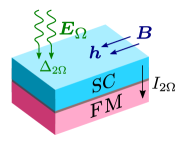
Figure 1: (a) Setup of the superconductor (SC) / ferromagnet (FM) structure. The exchange field $\bm{h}$ is induced by an external magnetic field $\bm{B}$. The double-frequency gap modulation can be excited by the external electromagnetic irradiation $\Delta_{2\Omega}\propto E_{\Omega}^{2}$ and is enhanced due to the coupling to the Higgs mode. (b) Sketch of the current generation by the time-dependent order parameter amplitude $\Delta(t)$. The shift of the gap amplitude $\delta\Delta(t)$ pushes occupied quasiparticle states up or down in energy. Due to the Zeeman shift $h$ the perturbation of the distribution function is asymmetric with respect to the Fermi level $\varepsilon_{F}$. This results in net spin and charge currents flowing into the attached ferromagnetic electrode (FM) through the tunnel barrier (I).

Setup. The considered setup is shown in Fig. 1(a). It consists of a superconducting (SC) film placed in contact with a ferromagnetic (FM) material. An effective spin splitting field $\bm{h}$ in SC is induced by an external in-plane magnetic field. Alternatively, $\bm{h}$ could be induced by the proximity to a ferromagnetic insulator Bergeret et al. (2001); Tokuyasu et al. (1988); Millis et al. (1988); Cottet et al. (2009); Eschrig et al. (2015). The system is exposed to external irradiation $E_{\Omega}e^{i\Omega t}$ which generates a time-dependent perturbation of the order parameter amplitude $\delta\Delta(t)=\Delta_{2\Omega}e^{2i\Omega t}$ through the second-order non-linearity $\Delta_{2\Omega}\propto E_{\Omega}^{2}$ Gorkov and Eliashberg (1968, 1969).

As shown in Fig. 1(b), the time-dependent gap function in the superconducting film creates a non-equilibrium state. Due to the Zeeman shift $h$ this state is non-symmetric with respect to the Fermi level $\varepsilon_{F}$ and therefore produces spin current through the tunnel barrier between the SC and the adjacent normal metal. This qualitative picture is based on the time-dependent energy spectrum $E=\sqrt{\xi_{p}^{2}+\Delta(t)^{2}}+\sigma h$ with $\sigma=\pm 1$ for spin-up/down Bogolubov quasiparticles respectively, where $\xi_{p}$ is the kinetic energy counted from the Fermi level $\varepsilon_{F}$.

For a slowly time-dependent order parameter we find the spin current

$$I_{s}(t)=\frac{\kappa}{\Gamma}\dot{\Delta}\frac{d}{d\Delta}(N_{+}-N_{-}),$$ (1)

where $\kappa$ is the effective barrier transparency, $N_{\sigma}(\Delta)$ is the equilibrium number of thermally excited quasiparticles in the spin-up/down subbands for the given order parameter $\Delta$. The spin current is determined by the energy relaxation Dynes parameter Dynes et al. (1984) $\Gamma$ and the result (1) is shown to be valid Sup for low frequencies $\Omega\ll\Gamma$. Expression (1) allows for the cartoon interpretation in terms of the semiconductor model in Fig. 1(b). However, for the most interesting case when the frequency of $\Delta(t)\propto e^{2i\Omega t}$ oscillation is comparable to the gap $\Omega\sim\Delta$ and hence is coupled to the Higgs mode Volkov and Kogan (1974); Kulik et al. (1981); Barankov et al. (2004); Barankov and Levitov (2006), the picture becomes more complicated. The exact expression for the time-dependent spin current valid for all frequencies is derived in this Letter [see Eq. (10)].

Second harmonic generation. Spin currents generated by the Higgs mode can be detected in various ways. The most common approaches for spin current detection are based on the inverse spin Hall effect and spin-filtering systems. Here we rely on the latter possibility which can be achieved by taking into account the spin-dependent transmission probability of the electrons through the SC/FM interface. In the setup shown in Fig. 1(a) the spin current is effectively converted to the charge current while passing through the spin-filtering barrier characterized by the polarization vector $\bm{P}$. The time-dependent charge current induced in this way by the order parameter amplitude oscillation is therefore qualitatively given by $I(t)\propto\bm{P}\cdot\bm{I}_{s}(t)$, which results in the estimate $I(t)\propto(\bm{P}\cdot\bm{h})\partial_{t}\Delta$. Modulation of the order parameter amplitude can be induced for example by an external irradiation Gorkov and Eliashberg (1968, 1969), $\Delta(t)\propto\bm{A}^{2}(t)$, where $\bm{A}(t)$ is the vector potential of the external field. Hence this charge current $I(t)\propto(\bm{P}\cdot\bm{h})\partial_{t}\bm{A}^{2}$, being quadratic in the vector potential, demonstrates the second harmonic generation (SHG) controlled by the superconducting order parameter.

Despite large attention to the non-linear effects in superconductors, SHG has not been obtained before . Hence only the third-harmonic generation has been studied in superconductors Gorkov and Eliashberg (1968, 1969); Amato and McLean (1976); Matsunaga et al. (2014); Giorgianni et al. (2019). We show below that such kind of SHG is not prohibited by the generic symmetries of the problem. However it is eliminated by the approximate symmetry of Fermi surface systems, made exact in the widely used quasiclassical approximation Silaev et al. (2017); qua . For the non-stationary charge current generated by the time-dependent vector potential this symmetry yields $I(\bm{A},\Delta)=-I(-\bm{A},\Delta^{*})$. Further, in the absence of supercurrent or external orbital fields we can assume the order parameter to be real $\Delta=\Delta^{*}$. Then even the broken inversion symmetry near surfaces does not help to produce SHG in superconducting systems in contrast to the normal metal counterpart of this effect, and the Higgs mode cannot be measured with this technique.

The particle-hole symmetry is broken to a large extent in SC/FM systems leading to large thermoelectric Machon et al. (2013); Ozaeta et al. (2014); Bergeret et al. (2018) and anomalous Josephson effects Silaev et al. (2017). As shown explicitly below for real $\Delta$ the tunnel charge current through the spin-polarized barrier satisfies the symmetry

$$I(\bm{A},\bm{h},\bm{P})=-I(-\bm{A},\bm{h},-\bm{P}).$$ (2)

In this case SHG is possible as can be seen from the expression for the tunnel current (2): Due to the requirement of the sign flip of $\bm{P}$ in the time reversal transformation, there is no longer a symmetry with respect to the mere flipping of the vector potential $\bm{I}(\bm{A})\neq-\bm{I}(-\bm{A})$. Hence for the ac external field $\bm{A}_{\Omega}e^{i\Omega t}$, Eq. (2) allows for the double-frequency charge current component $I_{2\Omega}e^{i\Omega t}$ with the amplitude $I_{2\Omega}\propto|\Delta|^{2}A^{2}_{\Omega}(\bm{P}\cdot\bm{h})$ as well as the dc tunnel current Virtanen et al. (2016) $I_{dc}\propto|\Delta|^{2}A_{\Omega}A_{-\Omega}(\bm{P}\cdot\bm{h})$.

Below we explicitly demonstrate the existence of the double-frequency spin and charge currents in SC/FM tunnel junctions subject to the external electromagnetic irradiation. We show that in general there are two contributions to such spin and charge SHG effect. One comes from the direct coupling of electrons in the superconductor to the vector potential. The other is induced by the order parameter amplitude modulation which in turn is excited by the electromagnetic irradiation.

Spin-polarized tunneling. We model the SC/FM junction using the tunneling Hamiltonian approach Ambegaokar and Baratoff (1963); Bardeen (1962) which has been extensively used to study both ac and dc tunnel currents Eckern et al. (1984); Harris (1975); Werthamer (1966); Ambegaokar and Baratoff (1963),

$$H_{T}=\sum_{kk^{\prime}\alpha}\check{A}_{k\alpha}^{\dagger}(\check{\Gamma}\hat{B}_{k^{\prime}})_{\alpha}+h.c.$$ (3)

$$\hat{\Gamma}={\cal T}\hat{\tau}_{3}+{\cal U}(\bm{m}\cdot\hat{\bm{\sigma}}).$$ (4)

Here $\hat{A}_{k\alpha}$ ($\hat{B}_{k\alpha}$) annihilates an electron with momentum $k$ and spin $\alpha$ in the superconductor (ferromagnet), the unit vector $\bm{m}$ defines the spin quantization axis of the barrier, $\hat{\tau}_{k}$ and $\hat{\sigma}_{k}$ are the Pauli matrices in Nambu and spin spaces, respectively, and $\cal U$ and $\cal T$ are the spin-independent and spin-dependent matrix elements of the tunneling Hamiltonian Bergeret et al. (2012a). The matrix tunneling current through the spin-polarized barriers can be expressed through momentum-averaged Green functions in the superconducting and ferromagnetic electrodes, $\nu_{S}\hat{g}_{S}=\hat{\tau}_{3}\sum_{k}\langle{\,\mathbb{T}}\hat{A}_{k}(t)\hat{A}^{\dagger}_{k}(t^{\prime})\rangle$ and $\nu_{F}\hat{g}_{F}=\hat{\tau}_{3}\sum_{k}\langle{\,\mathbb{T}}\hat{B}_{k}(t)\hat{B}^{\dagger}_{k}(t^{\prime})\rangle$, respectively. Here $t,\;t^{\prime}$ are imaginary times, $\mathbb{T}$ is the time-ordering operator, $\nu_{S/F}$ are the normal metal densities of states on the two sides of the junction. For simplicity we assume momentum-independent tunneling coefficients Bergeret et al. (2012a, b). The time-dependent tunneling current for the general non-equilibrium state in the electrodes Sup reads

$$\hat{I}(t)=i\frac{\nu_{S}\nu_{F}}{2}[{\hat{g}}_{S}\circ(\hat{\Gamma}{\hat{g}}_{F}\hat{\Gamma})-(\hat{\Gamma}{\hat{g}}_{F}\hat{\Gamma})\circ{\hat{g}}_{S}],$$ (5)

where ${\hat{g}}_{S(F)}$ is the quasiclassical GF in the SC (FM) electrode and $\circ$ denotes time convolution. The overall tunnel current amplitude is determined by $\kappa=\nu_{S}\nu_{F}({\cal T}^{2}+{\cal U}^{2})$ and the effective spin-filtering polarization is $\bm{P}=2{\cal T}{\cal U}\bm{m}/({\cal T}^{2}+{\cal U}^{2})$. Tracing the general expression with appropriate Pauli matrices we extract the charge current $I=e{\rm Tr}(\hat{\tau}_{3}\hat{I})$ and the spin current $\bm{I}_{s}={\rm Tr}(\hat{\bm{\sigma}}\hat{I})$, respectively.

We assume that the electrodes are described by the time-dependent quasiclassical Usadel theory and include only lowest order [$o(\kappa)$] corrections from tunneling Vadimov et al. (2019). This conventional approximation allows for the spin currents driven by the Higgs mode and external field even with a non-ferromagnetic barrier, that is at $P=0$. However, the direct coupling between the Higgs mode and the charge current is prohibited by the particle-hole symmetry. As shown in the Supplementary Material Sup for the solutions of Usadel equation this symmetry yields

$$\check{g}(\bm{A},\bm{h},\Delta)=-\hat{\tau}_{1}\check{g}(-\bm{A},\bm{h},\Delta^{*})\hat{\tau}_{1}.$$ (6)

Here the off-diagonal Nambu space Pauli matrix $\hat{\tau}_{1}$ interchanges the particle and hole blocks in the Hamiltonian Silaev et al. (2017). This symmetry is broken by the spin polarization of tunneling $P\neq 0$ so that the transformation (6) applied to the general tunnel current yields the relation (2) which allows for the finite charge current.

Further we assume that the SC electrode is driven out of equilibrium by the external irradiation. It generates the second-harmonic perturbation of the GF and tunnel current

$$\hat{g}_{S}(t,t^{\prime})=T\sum_{\omega}\hat{g}_{S}(\omega_{+},\omega_{-})e^{i\omega_{+}t-i\omega_{-}t^{\prime}}$$ (7)

$$\hat{I}({2\Omega})=iT\frac{\nu_{S}\nu_{F}}{2}\sum_{\omega}\hat{\Gamma}\hat{g}_{S}\hat{\Gamma}{\hat{g}}_{0}(\omega_{-})-{\hat{g}}_{0}(\omega_{+})\hat{\Gamma}\hat{g}_{S}\hat{\Gamma},$$ (8)

where $\omega_{\pm}=\omega\pm\Omega$ are the fermionic Matsubara frequencies shifted by the frequency $\Omega$ of the external field. We denote $\hat{g}_{S}=\hat{g}_{S}(\omega_{+},\omega_{-})$ and assume that the ferromagnet is in the equilibrium state determined by the GF $g_{F}(\omega)=g_{0}(\omega)\equiv{\rm sign}(\omega)\hat{\tau}_{3}$. There are two qualitatively different terms in the non-equilibrium GF $\hat{g}_{S}=\hat{g}_{\Delta}+\hat{g}_{AA}$. The first one is generated by the time-dependent order parameter whereas the second term is generated by the direct coupling to the external field. Below we discuss the corresponding contributions to the tunnel current and coupling to the Higgs mode.

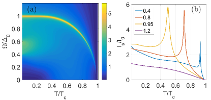
Figure 2: Amplitude of double-frequency spin current $I_{s}(2\Omega)e^{2i\Omega t}$ driven through the SC/FM tunnel junction by an external field $A_{\Omega}e^{i\Omega t}$. The current is normalized to $I_{0}=\kappa T_{c}D(eA_{\Omega}/c)^{2}$, where $T_{c}$ is the critical temperature. The sharp maximum at $\Omega=\Delta(T)$ corresponds to the resonant excitation of the Higgs mode. (a) $I_{s}(\Omega,T)$, (b) $I_{s}(T)$ at different frequencies $\Omega/\Delta_{0}=0.4;\;0.8;\;0.95;\;1.2$. The exchange field is $h=0.2\Delta_{0}$ and Dynes parameter $\Gamma=0.005\Delta_{0}$. The peaks are at temperatures determined by $\Omega=\Delta(T)$.

Higgs mode contribution. First, let us discuss the term $\hat{g}_{\Delta}$ which is generated by the time-dependent order parameter amplitude $\Delta_{2\Omega}e^{2i\Omega t}$. The correction to the GF driven by the time-dependent order parameter field is given by Sup

$$\hat{g}_{\Delta}=\Delta_{2\Omega}\frac{\hat{g}_{0}(\omega_{+})\hat{\tau}_{2}\hat{g}_{0}(\omega_{-})-\hat{\tau}_{2}}{s(\omega_{+})+s(\omega_{-})},$$ (9)

where the Nambu-space Pauli matrix $\hat{\tau}_{2}$ is the vertex describing the coupling of electrons to the order parameter field. In this expression the denominator contains $s(\omega)=[(\omega+i\sigma h)^{2}+\Delta^{2}]^{1/2}$, where $\sigma=+/-$ corresponds to spin-up/down subbands. Substituting Eq. (9) to the general matrix current (5) and using analytical continuation Kopnin (2001); Sup we obtain the amplitude of real-frequency spin current $I_{s}(2\Omega)e^{2i\Omega t}$

$$I_{s}=i\kappa\Delta_{2\Omega}\Delta\sum_{\sigma}\sigma\int\frac{d\varepsilon}{4\pi}\frac{\varepsilon[n(\varepsilon_{+})-n(\varepsilon_{-})]}{s^{R}_{+}s^{A}_{-}(s^{R}_{+}+s^{A}_{-})},$$ (10)

where $n(\varepsilon)$ is the equilibrium distribution function, $\varepsilon_{\pm}=\varepsilon\pm\Omega+\sigma h$ and $s^{R,A}=-i\sqrt{(\varepsilon\pm i\Gamma)^{2}-\Delta^{2}}$.

In the low-frequency limit $\Omega\ll\Gamma$ we restore Eq. (1) when the spin current is driven by the adiabatic time dependence of $\Delta$ in accordance with the qualitative picture shown schematically in Fig. 1(b). The numbers of thermally excited states are $N_{\sigma}=\int d\xi_{p}n(E_{\sigma}(\xi_{p},\Delta))$ where $E_{\sigma}=\sqrt{\xi_{p}^{2}+\Delta^{2}}+\sigma h$ is the spin-splitted spectrum of Bogolubov quasiparticles.

In the presence of the Higgs mode, that is the slowly decaying oscillations of the order parameter $\Delta(t)$ Volkov and Kogan (1974); Barankov et al. (2004), the spin current is given by the sum of the corresponding Fourier components with the amplitudes given by (10). As a result of Eq. (10) we get slowly-decaying oscillations of the spin current $I_{s}(t)$ which can be measured using electrical probes after the superconductor is initially driven into a non-equilibrium state by a field pulse.

Coupling to an external field. The Higgs mode can also be revealed by the spin current if the superconductor is driven out of equilibrium by a continuous wave irradiation as shown schematically in Fig. 1(a). The second-order direct coupling to the external field is determined by the GF perturbation $\hat{g}_{AA}\propto A_{\Omega}^{2}$. In the dirty limit this term can be found from the Usadel equation as described in the Supplementary Material Sup

$$\hat{g}_{AA}=D\left(\frac{eA_{\Omega}}{c}\right)^{2}\frac{\hat{\tau}_{3}\hat{g}_{0}(\omega)\hat{\tau}_{3}-\hat{g}_{0}(\omega_{+})\hat{\tau}_{3}\hat{g}_{0}(\omega)\hat{\tau}_{3}\hat{g}_{0}(\omega_{-})}{s(\omega_{+})+s(\omega_{-})},$$ (11)

where $D$ is the diffusion coefficient.

This coupling to the external field has a twofold effect. First it directly generates second-harmonic spin and charge currents. Besides that it generates the time-dependent component of the order parameter according to the self-consistency equation. The bare amplitude of the order parameter perturbation $F_{\Delta}e^{2i\Omega t}$ is given by $F_{\Delta}=-\lambda T\sum_{\omega}{\rm Tr}[\hat{\tau}_{2}\hat{g}_{AA}]$, where $\lambda$ is the coupling constant of superconductivity and the Pauli matrix $\hat{\tau}_{2}$ corresponds to the superconducting amplitude vertex.

The resonant excitation of the total order parameter amplitude is determined by the equation with polarization corrections $\Delta_{2\Omega}=F_{\Delta}+\Pi(2\Omega)\Delta_{2\Omega}$, where $\Pi(\Omega)$ is the order parameter polarization operator Tsuji and Aoki (2015b); Cea et al. (2016). It has the simple solution $\Delta_{2\Omega}=F_{\Delta}/[1-\Pi(2\Omega)]$, that yields the resonance condition for $\Omega=\Delta$ when the denominator satisfies $1-\Pi(2\Delta)=0+o(\sqrt{\Gamma})$. Hence the maximal amplitude of the spin current is determined by the broadening parameter $\Gamma$, leading to a sharp peak in $I_{s}(\Omega,T)$ for $\Omega\approx\Delta(T)$. This behaviour of the spin current is illustrated in Fig. 2. The charge current appearing in the case of a finite spin polarization of the barrier is given by $I=e\bm{P}\cdot\bm{I}_{s}$, where the spin current vector is $\bm{I}_{s}=I_{s}\bm{h}/h$.

Figure 3: The setups to study transverse spin currents coupled to the Higgs mode in the superconductor (S). The exchange field in S is generated by the adjacent ferromagnetic insulator (FI) with magnetization $\bm{m}_{0}$. (a) The spin torque $\bm{\tau}$ is generated in an adjacent ferromagnet (F) with non-collinear magnetization $\bm{m}\nparallel\bm{m}_{0}$. (b) Magnetization precession $\bm{m}(t)$ induces the spin current $\bm{I}_{s}$ and the spin battery effect leading to a perturbation of the order parameter amplitude $\delta\Delta$.

Spin torques. If the exchange field $\bm{h}$ in the SC is non-collinear with the magnetization $\bm{m}$ in the FM, the Higgs mode generates a spin torque acting on $\bm{m}$. The generic system which can realize this configuration is shown in Fig. 3(a). Here the exchange field $\bm{h}\parallel\bm{m}_{0}$ is created by the ferromagnetic insulator (FI) layer with a fixed magnetic moment $\bm{m}_{0}$ Bergeret et al. (2018).

First let us discuss the STT generated by the Higgs mode as shown schematically in Fig. 3(a). The polarization of the non-equilibrium spin current $\bm{I}_{s}$ in the superconductor electrode depends only on the direction of the exchange field $\bm{h}$ and is not sensitive to the magnetic moment $\bm{m}$ in the adjacent FM. This is in contrast to the equilibrium components of the spin current which exist in such systems with non-collinear magnetic moments Silaev et al. (2015b) even without the external drive, and are proportional to $\propto\bm{h}\times\bm{m}$. Assuming that the transverse component of the spin current is absorbed in the ferromagnet Tserkovnyak et al. (2005); Slonczewski (1996); Brataas et al. (2000); Waintal et al. (2000); Stiles and Zangwill (2002) we obtain the STT $\bm{\tau}=I_{s}\bm{h}_{\perp}/h$ where $\bm{h}_{\perp}=\bm{h}-\bm{m}(\bm{m}\cdot\bm{h})$ is the perpendicular component of the exchange field.

This effect can be viewed as the Higgs-mode mediated transfer of the spin angular momentum from the FI to the metallic ferromagnet shown in Fig. 3(a). Oscillating STT generated by the order parameter amplitude mode can excite the ferromagnetic resonance (FMR) in the attached ferromagnet. Hybridization of FMR and Higgs resonances should show up as the avoided crossing of the peaks in the second-harmonic response of the systems shown in Fig.3a. Such experiment will directly demonstrate the dynamical coupling of the magnetic and superconducting orders. Modification of FMR resonance linewidth by superconducting correlations in FM/SC structures has been observed recentlyBell et al. (2008); Jeon et al. (2018).

Experimentally this effect can be realized using nanomagnets Yakushiji et al. (2005); Krause et al. (2007); Loth et al. (2010); Krause et al. (2016) because in these small-sized systems one can achieve larger coupling between FMR and Higgs mode. The other alternative is to use molecular magnets coupled to the superconductor and observe the spin currents using macroscopic quantum tunnelling effectThomas et al. (1996).

The reciprocal effect which results in the generation of the gap function amplitude perturbation $\delta\Delta$ by the magnetic precession is shown in Fig. 3(b). To demonstrate the possibility to induce $\delta\Delta(t)$ by magnetic precession we assume that the spin current $\bm{I}_{s}\propto\bm{m}\times\dot{\bm{m}}$ is pumped by the time-dependent magnetization $\bm{m}(t)$ in the FM Tserkovnyak et al. (2005). This spin current has a longitudinal component $\bm{I}_{s}\parallel\bm{h}$ which generates a spin accumulation in the superconductor. For a low frequency of the magnetic precession this effect can be described by the spin-dependent chemical potential shift $\mu_{s}$ in the SC. In combination with the spin-splitting field $\bm{h}$ the spin accumulation results in a perturbation of the gap function amplitude Virtanen et al. (2016); Bobkova and Bobkov (2017)

$$\delta\Delta=\frac{\lambda\Delta}{1-\Pi}\mu_{s}\partial_{\Delta}(N_{+}-N_{-}),$$ (12)

where $1-\Pi\propto\lambda$ is the low-frequency asymptotic of the polarization operator. This expression demonstrates the possibility to couple the order parameter amplitude with the magnetization dynamics. Thus the higher-frequency magnetization precession with $\Omega\sim\Delta$ generates the Higgs mode in the superconductor with a spin-splitting field.

Conclusions. In this Letter, we have demonstrated that spin currents can be effectively generated by the collective amplitude modes of the superconducting order parameter. Owing to the fact that the Higgs mode can be generated by the external irradiation Silaev (2019b); Murotani and Shimano (2019), our result paves the way for conceptually new direction of superconducting optospintronics – the study of spin currents and spin torques generated by light interacting with superconducting materials.

We have suggested a detection scheme for the Higgs mode based on measuring resonant electric signals, either the charge current or voltage generated across the spin-polarized tunnel junction by the external field. Because these signals appear at the doubled frequency of the external field, our setup introduces the system featuring the SHG effect controlled by superconductivity. The suggested SHG effect can be studied using optical or microwave detectors. Being sensitive to the magnitude of the spin splitting field and the quality of the spin-polarized barriers, this effect provides a tool for the diagnostics of large-area SC/FM junctions suggested to be used as a new platform for the fabrication of radiation sensors Heikkilä et al. (2018). The ac tunneling current $I_{2\Omega}$ can be detected using electrical probes allowing for electrical detection of the Higgs mode in superconductors.

Acknowledgements This work was supported by the Academy of Finland (Projects No. 297439 and 317118), Jenny and Antti Wihuri Foundation, Russian Science Foundation (Grant No. 19-19-00594) and from the European Union’s Horizon 2020 research and innovation programme under grant agreement No 800923 (SUPERTED).

I Supplementary

I.1 Tunnel current

We model SC/I/FM junction by the tunneling Hamiltonian:

$$H_{T}=\sum_{kk^{\prime}\alpha}\check{A}_{k\alpha}^{\dagger}(\check{\Gamma}\hat{B}_{k^{\prime}})_{\alpha}+h.c.$$ (13)

$$\hat{\Gamma}={\cal T}\tau_{3}+{\cal U}(\bm{m}\bm{\sigma})$$ (14)

where the unit vector $\bm{m}$ is the spin-filtering axis of the barrier. This model describes spin-dependent tunnelling through the SC/FM interface Bergeret et al. (2012a). We calculate the tunneling current as a function of the time on the contour running along the imaginary time axis from $0$ to $\beta=1/T$. The matrix tunneling current in terms of the imaginary-time functions reads

$$\hat{I}(t)=\frac{i}{2}\sum_{k}\left[\partial_{t}\hat{G}_{S}(t,t^{\prime},k,k)+\partial_{t^{\prime}}\hat{G}_{S}(t,t^{\prime},k,k)\right]|_{t=t^{\prime}}.$$ (15)

To find the perturbation we consider the contour-ordered GF

$$\hat{G}_{S}(t,t^{\prime},k,k^{\prime})=\langle\,\mathbb{T}\hat{S}\hat{A}_{k}(t)\hat{A}^{\dagger}_{k^{\prime}}(t^{\prime})\rangle,$$ (16)

where $\mathbb{T}$ is the contour-ordering operator and

$$\hat{S}\approx 1-\int_{0}^{\beta}dt_{c}H_{T}(t_{c}).$$ (17)

In the interaction representation with respect to the tunneling Hamiltonian the equation of motion is

$$\partial_{t}\check{A}_{k}=[\check{A}_{k},H_{T}]=\sum_{k^{\prime}}(\check{\Gamma}_{kk^{\prime}}\hat{B}_{k^{\prime}})$$ (18)

Using the equation of motion we get

$$\partial_{t}\hat{G}_{S}(t,t^{\prime},\bm{k},\bm{k})=\sum_{q}\langle\,\mathbb{T}\hat{S}[\hat{\Gamma}_{kq}\check{B}_{q}(t)]\check{A}^{\dagger}_{k\beta}(t^{\prime})\rangle\approx$$ (19)

$$-\sum_{q}\langle\,\mathbb{T}\int_{0}^{\beta}dt_{c}H_{T}(t_{c})\hat{\Gamma}_{kq}\check{B}_{q}(t)\check{A}^{\dagger}_{k}(t^{\prime})\rangle=$$ (20)

$$-\sum_{k_{1},k^{\prime}_{1},q}\langle\,\mathbb{T}\int_{0}^{\beta}dt_{c}[\check{B}^{\dagger}_{k^{\prime}_{1}}(t_{c})\hat{\Gamma}^{\dagger}_{k_{1}k^{\prime}_{1}}]\check{A}_{k_{1}}(t_{c})[\hat{\Gamma}_{kq}\check{B}_{q}(t)]\check{A}^{\dagger}_{k}(t^{\prime})\rangle=$$

$$-\sum_{k_{1},k^{\prime}_{1},q}\int_{0}^{\beta}dt_{c}\{\hat{\Gamma}\langle\,\mathbb{T}\check{B}_{q}(t)\check{B}^{\dagger}_{k^{\prime}_{1}}(t_{c})\rangle\hat{\Gamma}(t_{c})\}\langle\,\mathbb{T}\check{A}_{k_{1}}(t_{c})\check{A}^{\dagger}_{k}(t^{\prime})\rangle=$$

$$-\sum_{k_{1},k_{1}^{\prime},q}\int_{0}^{\beta}dt_{c}\hat{\Gamma}_{kq}{\hat{G}}_{F}(t,t_{c},q,\bm{k}_{1})\hat{\Gamma}_{\bm{k}^{\prime}_{1}k_{1}}{\hat{G}}_{S}(t_{c},t^{\prime},\bm{k}^{\prime}_{1},\bm{k})$$

and

$$\partial_{t^{\prime}}\hat{G}_{S}(t,t^{\prime},\bm{k},\bm{k})=\sum_{q}\langle\,\mathbb{T}\hat{S}\check{A}_{k}(t)[\hat{\Gamma}_{kq}\check{B}_{q}(t^{\prime})]^{\dagger}\rangle\approx$$ (21)

$$-\sum_{q}\langle\,\mathbb{T}\int_{0}^{\beta}dt_{c}H_{T}(t_{c})\check{A}_{k}(t)[\hat{\Gamma}_{kq}\check{B}_{q}(t^{\prime})]^{\dagger}\rangle=$$

$$-\sum_{k_{1},k^{\prime}_{1},q}\langle\,\mathbb{T}\int_{0}^{\beta}dt_{c}[\hat{\Gamma}_{k_{1}k_{1}^{\prime}}\check{B}_{k^{\prime}_{1}}(t_{c})]\check{A}^{\dagger}_{k_{1}}(t_{c})\check{A}_{k}(t)[\check{B}^{\dagger}_{q}(t^{\prime})\hat{\Gamma}^{\dagger}_{qk}]\rangle=$$

$$\sum_{k_{1},k^{\prime}_{1},q}\int_{0}^{\beta}dt_{c}\langle\,\mathbb{T}\check{A}_{k}(t)\check{A}^{\dagger}_{k_{1}}(t_{c})\rangle\{\hat{\Gamma}_{k_{1}k^{\prime}_{1}}\langle\,\mathbb{T}\check{B}_{k^{\prime}_{1}}(t_{c})\check{B}^{\dagger}_{q}(t^{\prime})\rangle\hat{\Gamma}_{qk}\}=$$

$$\sum_{k_{1},k^{\prime}_{1},q}\int_{0}^{\beta}dt_{c}{\hat{G}}_{S}(t,t_{c},\bm{k},\bm{k}_{1})\hat{\Gamma}_{k_{1}\bm{k}_{1}^{\prime}}{\hat{G}}_{F}(t_{c},t^{\prime},\bm{k}_{1}^{\prime},q)\hat{\Gamma}_{q,k}.$$

Hence the matrix current is given by

$$\hat{I}(t)=\frac{i}{2}\sum_{k,k_{1},k_{1}^{\prime},q}$$ (22)

$$\int_{0}^{\beta}dt_{c}\{{\hat{G}}_{S}(t,t_{c},\bm{k},\bm{k}_{1})\hat{\Gamma}_{k_{1}\bm{k}_{1}^{\prime}}{\hat{G}}_{F}(t_{c},t,\bm{k}_{1}^{\prime},\bm{q})\hat{\Gamma}_{qk}$$

$$-\int_{0}^{\beta}dt_{c}\hat{\Gamma}_{k,q}{\hat{G}}_{F}(t,t_{c},\bm{q},\bm{k}_{1})\hat{\Gamma}_{k_{1}\bm{k}_{1}^{\prime}}{\hat{G}}_{S}(t_{c},t,\bm{k}_{1}^{\prime},\bm{k})\}.$$

We assume that GFs are spatially homogeneous, so that ${\hat{G}}_{F}(t,t_{c},\bm{q},\bm{k}_{1})=\delta_{q,k_{1}}\hat{\Gamma}{\hat{G}}_{F}(t,t_{c},\bm{q})$ and the matrix element is momentum-independent $\hat{\Gamma}_{kk^{\prime}}=\hat{\Gamma}$. Then we can introduce the quasiclassical functions $\sum_{q}{\hat{G}}_{F,S}(t,t_{c},\bm{q})=\nu_{F,S}\hat{\tau}_{3}\hat{g}_{F,S}(t,t_{c})$ to write the current as

$$\hat{I}(t)=i\frac{\nu_{S}\nu_{F}}{2}[{\hat{g}}_{S}\circ(\hat{\tau}_{3}\hat{\Gamma}{\hat{g}}_{F}\hat{\Gamma}\hat{\tau}_{3})-(\hat{\tau}_{3}\hat{\Gamma}{\hat{g}}_{F}\hat{\Gamma}\hat{\tau}_{3})\circ{\hat{g}}_{S}],$$ (23)

where the time convolution symbol is defined as $(A\circ B)(t,t_{1})=\int_{0}^{\beta}dt_{c}A(t,t_{c})B(t_{c},t)$. Taking into account that the normal metal GF ${\hat{g}}_{F}$ commutes with $\hat{\tau}_{3}$, Eq. (23) can be reduced to Eq. (5) in the main text.

I.2 Analytical continuation

In order to find the real-frequency response we need to implement the analytic continuation of Eq. (8). These second-order responses are obtained by the summation of expressions which depend on the multiple shifted fermionic frequencies such as $g(\omega_{1},\omega_{2},\omega_{3})$. The analytic continuation of the sum by Matsubara frequencies is determined according to the general rule Kopnin (2001)

$$T\sum_{\omega}g(\omega_{1},\omega_{2},\omega_{3})\to$$ (24)

$$\sum_{l=1}^{3}\int\frac{d\varepsilon}{4\pi i}n_{0}(\varepsilon_{l})\left[g(...,-i\varepsilon^{R}_{l},...)-g(...,-i\varepsilon^{A}_{l},...)\right],$$

where $n_{0}(\varepsilon)=\tanh(\varepsilon/2T)$ is the equilibrium distribution function. In the r.h.s. of (24) we substitute in each term $\omega_{k<l}=-i\varepsilon^{R}_{k}$ and $\omega_{k>l}=-i\varepsilon^{A}_{k}$ for $k=1,2,3$, denote $\varepsilon_{k}=\varepsilon+(2-k)\Omega$ and $\varepsilon^{R}=\varepsilon+i\Gamma$, $\varepsilon^{A}=\varepsilon-i\Gamma$. Here the term with $\Gamma>0$ is added to shift the integration contour into the corresponding half-plane. At the same time, $\Gamma$ can be used as the Dynes parameter Dynes et al. (1984) to describe the effect of different depairing mechanisms on spectral functions in the superconductor. We implement the analytical continuation in such a way that $s(-i\varepsilon^{R,A})=-i\sqrt{(\varepsilon^{R,A})^{2}-\Delta^{2}}$ assuming that the branch cuts run from $(\Delta,\infty)$ and $(-\infty,-\Delta)$. In the presence of the spin-splitting field the energy in Eq. (24) should be shifted to $\varepsilon+\sigma h$, where $\sigma=\pm 1$ is the spin subband index.

Equilibrium GF in the imaginary frequency domain is given by $\hat{g}_{0}(\omega)=(\hat{\tau}_{3}\omega-\hat{\tau}_{2}\Delta)/s(\omega)$. The real-frequency continuation reads $\hat{g}^{R,A}_{0}(\varepsilon)=(\hat{\tau}_{3}\varepsilon_{R,A}-i\hat{\tau}_{2}\Delta)/\sqrt{(\varepsilon^{R,A})^{2}-\Delta^{2}}$.

Example. To demonstrate the analytical continuation in practice we calculate the spin current driven by the Higgs mode. For real frequencies the spin current obtained from (23) can be written in terms of the Keldysh component

$$I_{s}=\frac{\kappa}{8\pi}\sum_{\sigma}\sigma\int d\varepsilon{\rm Tr}[\hat{g}_{F}(\varepsilon_{+})\hat{g}_{S}(\varepsilon)-\hat{g}_{S}(\varepsilon)\hat{g}_{F}(\varepsilon_{-})]^{K}=$$

$$\frac{\kappa}{8\pi}\sum_{\sigma}\sigma\int d\varepsilon[n(\varepsilon_{+})-n(\varepsilon_{-})]{\rm Tr}[\hat{\tau}_{3}g^{a}_{S}],$$ (25)

where $\varepsilon_{\pm}=\varepsilon+\sigma h\pm\omega$. In deriving (25) we used the fact that $\hat{g}^{R(A)}_{F}=\pm 1$ do not dependent on energy. The anomalous part of the nonequilibrium GF in the superconductor is

$${g}^{a}_{S}=\Delta_{2\Omega}\frac{g^{R}(\varepsilon_{+})\tau_{2}g^{A}(\varepsilon_{-})-\tau_{2}}{s^{R}_{+}+s^{A}_{-}}$$ (26)

where we denote $s^{R,A}_{\pm}=s^{R,A}(\varepsilon_{\pm})$.

Substituting the solution (26) and using ${\rm Tr}[\tau_{3}g^{R}_{+}\tau_{2}g^{A}_{-}]=2i\Delta_{0}\varepsilon/s^{R}_{+}s^{A}_{-}$, we get

$$I_{s}=i\kappa\Delta_{0}\Delta_{2\Omega}\sum_{\sigma}\sigma\int\frac{d\varepsilon}{4\pi}\frac{(\varepsilon+\sigma h)[n(\varepsilon_{+})-n(\varepsilon_{-})]}{s^{R}_{+}s^{A}_{-}(s^{R}_{+}+s^{A}_{-})}=$$ (27)

$$\frac{i\kappa\Delta_{0}\Delta_{2\Omega}}{(\omega+i\Gamma)}\int\frac{d\varepsilon}{16\pi}\sum_{\sigma}\sigma[n(\varepsilon_{+})-n(\varepsilon_{-})]\left(\frac{1}{s^{R}_{+}}-\frac{1}{s^{A}_{-}}\right),$$

where we use $(s^{R}_{+})^{2}-(s^{A}_{-})^{2}=4(\varepsilon+\sigma h)(\omega+i\Gamma)$. In the low-frequency limit we can substitute $n(\varepsilon_{+})-n(\varepsilon_{-})=2\omega\partial_{\varepsilon}n$ and ${s^{R}_{+}}=-{s^{A}_{+}}=-i\sqrt{\varepsilon^{2}-\Delta^{2}}$. Then spin current can be written in the simple form

$$I_{s}=\frac{\kappa}{\Gamma}\sum_{\sigma}\sigma\frac{d}{dt}\int d\xi_{p}n(E_{\sigma}(\xi_{p},\Delta(t)))=\frac{\kappa}{\Gamma}\dot{\Delta}\frac{d}{d\Delta}(N_{+}-N_{-})$$ (28)

where $E_{\sigma}(\xi_{p},\Delta(t))=\sqrt{\xi_{p}^{2}+\Delta^{2}(t)}+\sigma h$ is the spectrum of Bogolubov quasiparticles shifted by the spin-splitting field $h$.

I.3 Description in terms of the time-dependent Usadel equation

We start by analyzing the symmetries of the current in a superconductor driven by the time-dependent external field vector potential $\bm{A}(\bm{r},t)$, order parameter $\Delta(\bm{r},t)$ and exchange field $\bm{h}(\bm{r},t)$. Superconductor is described by Usadel equation, which is a diffusion-like equation for the quasiclassical Green functions (GF). In the imaginary time representation it has the form

$$-i\{\hat{\tau}_{3}\partial_{\tau},\check{g}\}_{\tau}=D\hat{\partial}_{\bf r}(\check{g}\circ\hat{\partial}_{\bf r}\check{g})-i[\hat{\tau}_{3}\hat{H},\check{g}]_{t}$$ (29)

where $D$ is the diffusion constant, $\hat{H}=\Delta\hat{\tau}_{1}+\bm{\sigma}\bm{h}$. Here $\hat{\tau}_{i}$ and $\hat{\sigma}_{i}$ ($i=0,1,2,3$) are Pauli matrices in Nambu and spin space, $h$ is the exchange field. The (anti)commutator, convolution product and differential superoperator in Eq. (29) are

$$\{\hat{\tau}_{3}\partial_{\tau},\check{g}\}_{\tau} =\hat{\tau}_{3}\partial_{\tau_{1}}\check{g}(\tau_{1},\tau_{2})+\partial_{\tau_{2}}\check{g}(\tau_{1},\tau_{2})\hat{\tau}_{3},$$ (30)

$$(f\circ g)(\tau_{1},\tau_{2}) =\int_{0}^{\beta}d{\tau_{3}}f(\tau_{1},\tau_{3})g(\tau_{3},\tau_{2}),$$ (31)

$$\hat{\partial}_{\bm{r}} =\partial_{\bm{r}}-ie[\hat{\tau}_{3}A(t),\cdot\;].$$ (32)

Equation (29) is complemented by the normalization condition $\check{g}\circ\check{g}=1$. The bulk charge current is given by

$${\bm{j}}(t)=i\frac{\sigma_{n}}{8e}{\rm Tr}[\hat{\tau}_{3}\check{g}\circ\hat{\partial}_{\bm{r}}\check{g}],$$ (33)

where $\sigma_{n}=e^{2}\nu_{0}D$ is the normal metal conductivity and $\nu_{0}$ is the density of states at the Fermi level.

Direct coupling to the vector potential. In the dirty limit we can find corrections from the Usadel equation. In the frequency domain $\hat{g}_{AA}(\tau,\tau^{\prime})=e^{i(\omega_{+}\tau-\omega_{-}\tau^{\prime})}D\left(\frac{eA_{\Omega}}{c}\right)^{2}\hat{g}_{AA}$ that yields

$$s_{+}\hat{g}_{0}(\omega_{+})\hat{g}_{AA}-s_{-}\hat{g}_{AA}\hat{g}_{0}(\omega_{-})=$$ (34)

$$[\hat{g}_{0}(\omega_{+})\tau_{3}\hat{g}_{0}(\omega)\tau_{3}-\tau_{3}\hat{g}_{0}(\omega)\tau_{3}\hat{g}_{0}(\omega_{-})],$$

where we denote again $\omega_{\pm}=\omega\pm\Omega$. The solution of this equation can be written as

$$g_{AA}=\frac{\hat{\tau}_{3}\hat{g}_{0}(\omega)\hat{\tau}_{3}-\hat{g}_{0}(\omega_{+})\hat{\tau}_{3}\hat{g}_{0}(\omega)\hat{\tau}_{3}\hat{g}_{0}(\omega_{-})}{s_{+}+s_{-}}.$$ (35)

Contribution of the Higgs mode. Besides the corrections to the GF induced directly by the electromagnetic field we need to take into account the time-dependent order parameter amplitude which drives the system out of equilibrium.

The first order correction due to the external gap perturbation $\Delta_{2\Omega}e^{2i\Omega t}$ is

$$\hat{g}_{\Delta}=\Delta_{2\Omega}\frac{\hat{g}_{0}(\omega_{+})\hat{\tau}_{2}\hat{g}_{0}(\omega_{-})-\hat{\tau}_{2}}{s_{+}+s_{-}},$$ (36)

where $s_{\pm}=s(\omega_{\pm})$ and $\omega_{\pm}=\omega\pm\Omega$.

The order parameter amplitude in turn is perturbed by the electric field which induces the corrections to the GF $\hat{g}_{AA}$ found above in Eq. (35). First we calculate the direct coupling of the order parameter amplitude to the external field described by the response function

$$F_{\Delta}(2\Omega)=-\lambda T\sum_{\omega}{\rm Tr}[\hat{\tau}_{2}\hat{g}_{AA}]$$ (37)

where we introduce the dimensionless pairing constant $\lambda$. To find the total order parameter perturbation it is crucial to renormalise the response by the corrections described by the polarization operator $\tilde{\Delta}=F_{\Delta}/(1-\Pi)$

$$\Pi(\Omega)=1+2\pi\lambda T\sum_{\omega}\frac{\Delta^{2}+\Omega^{2}}{s(\omega)(\omega^{2}-\Omega^{2})}.$$ (38)

Assuming that order parameter has frequency $2\Omega$ we can find the corresponding perturbation of the GF

$$\hat{g}_{\Delta}(\tau,\tau^{\prime})=\sum_{\omega}\hat{g}_{\Delta}e^{i\omega_{+}\tau-i\omega_{-}\tau^{\prime}}$$ (39)

The first order correction to the external gap perturbation $F_{\Delta}$ is given by

$$\hat{g}_{\Delta}=\frac{F_{\Delta}}{1-\Pi(2\Omega)}\frac{\hat{g}_{0}(\omega_{+})\hat{\tau}_{2}\hat{g}_{0}(\omega_{-})-\hat{\tau}_{2}}{s_{+}+s_{-}}.$$ (40)

I.4 Symmetries of the solutions and the current as functions of macroscopic fields

Particle-hole symmetry. The time-dependent quasiclassical Eq. (29) has the particle-hole symmetry which yields the general relation for the momentum-averaged GF

$$\check{g}(\bm{A},\bm{h},\Delta)=-\hat{\tau}_{1}\check{g}(-\bm{A},\bm{h},\Delta^{*})\hat{\tau}_{1}.$$ (41)

Artificial BdG symmetry. The weak-coupling theory of superconductivity based on the BdG equation yields an additional symmetry of the spectrum and GF determined by the transformation

$$\check{g}(\bm{A},\bm{h},\Delta)=-\hat{\sigma}_{2}\hat{\tau}_{1}\check{g}^{\intercal}(\bm{A},\bm{h},\Delta)\hat{\tau}_{1}\hat{\sigma}_{2}.$$ (42)

Here we introduce the generalized transposition operator $\intercal$ which interchanges all indices including time. This transformation leaves the Usadel equation invariant. Besides that it also leaves invariant both the bulk and tunnel currents and therefore it does not provide any additional constraints for the non-linear responses.

References

- Varma (2002) C. M. Varma, J. Low Temp. Phys. 126, 901 (2002).
- Podolsky et al. (2011) D. Podolsky, A. Auerbach, and D. P. Arovas, Phys. Rev. B 84, 174522 (2011).
- Pashkin and Leitenstorfer (2014) A. Pashkin and A. Leitenstorfer, Science 345, 1121 (2014).
- Volovik and Zubkov (2014) G. E. Volovik and M. A. Zubkov, J. Low Temp. Phys. 175, 486 (2014).
- Pekker and Varma (2015) D. Pekker and C. Varma, Annu. Rev. Condens. Matter Phys. 6, 269 (2015).
- Higgs (1964) P. W. Higgs, Phys. Rev. Lett. 13, 508 (1964).
- Grüner (1988) G. Grüner, Rev. Mod. Phys. 60, 1129 (1988).
- Paulson et al. (1973) D. N. Paulson, R. T. Johnson, and J. C. Wheatley, Phys. Rev. Lett. 30, 829 (1973).
- Lawson et al. (1973) D. T. Lawson, W. J. Gully, S. Goldstein, R. C. Richardson, and D. M. Lee, Phys. Rev. Lett. 30, 541 (1973).
- Zavjalov et al. (2016) V. V. Zavjalov, S. Autti, V. B. Eltsov, P. J. Heikkinen, and G. E. Volovik, Nat. Comm. 7, 10294 (2016).
- Bissbort et al. (2011) U. Bissbort, S. Götze, Y. Li, J. Heinze, J. S. Krauser, M. Weinberg, C. Becker, K. Sengstock, and W. Hofstetter, Phys. Rev. Lett. 106, 205303 (2011).
- Endres et al. (2012) M. Endres, T. Fukuhara, D. Pekker, M. Cheneau, P. Schauß, C. Gross, E. Demler, S. Kuhr, and I. Bloch, Nature 487, 454 (2012).
- Volkov and Kogan (1974) A. F. Volkov and S. M. Kogan, JETP 38, 1018 (1974), [Zh. Eksp. Teor. Fiz. 65, 2038 (1973)].
- Sooryakumar and Klein (1980) R. Sooryakumar and M. V. Klein, Phys. Rev. Lett. 45, 660 (1980).
- Littlewood and Varma (1982a) P. B. Littlewood and C. M. Varma, Phys. Rev. B 26, 4883 (1982a).
- Barankov et al. (2004) R. A. Barankov, L. S. Levitov, and B. Z. Spivak, Phys. Rev. Lett. 93, 160401 (2004).
- Grasset et al. (2018) R. Grasset, T. Cea, Y. Gallais, M. Cazayous, A. Sacuto, L. Cario, L. Benfatto, and M.-A. Méasson, Phys. Rev. B 97, 094502 (2018).
- Matsunaga et al. (2013) R. Matsunaga, Y. I. Hamada, K. Makise, Y. Uzawa, H. Terai, Z. Wang, and R. Shimano, Phys. Rev. Lett. 111, 057002 (2013).
- Matsunaga et al. (2014) R. Matsunaga, N. Tsuji, H. Fujita, A. Sugioka, K. Makise, Y. Uzawa, H. Terai, Z. Wang, H. Aoki, and R. Shimano, Science 345, 1145 (2014).
- Sherman et al. (2015) D. Sherman, U. S. Pracht, B. Gorshunov, S. Poran, J. Jesudasan, M. Chand, P. Raychaudhuri, M. Swanson, N. Trivedi, A. Auerbach, M. Scheffler, A. Frydman, and M. Dressel, Nature Physics 11, 188 (2015).
- Tsuji and Aoki (2015a) N. Tsuji and H. Aoki, Phys. Rev. B 92, 064508 (2015a).
- Matsunaga et al. (2017) R. Matsunaga, N. Tsuji, K. Makise, H. Terai, H. Aoki, and R. Shimano, Phys. Rev. B 96, 020505 (2017).
- Katsumi et al. (2018) K. Katsumi, N. Tsuji, Y. I. Hamada, R. Matsunaga, J. Schneeloch, R. D. Zhong, G. D. Gu, H. Aoki, Y. Gallais, and R. Shimano, Phys. Rev. Lett. 120, 117001 (2018).
- Nakamura et al. (2018) S. Nakamura, Y. Iida, Y. Murotani, R. Matsunaga, H. Terai, and R. Shimano, “Infrared activation of higgs mode by supercurrent injection in a superconductor nbn,” (2018), arXiv:1809.10335 .
- Uematsu et al. (2018) H. Uematsu, T. Mizushima, A. Tsuruta, S. Fujimoto, and J. A. Sauls, “Chiral higgs mode in nematic superconductors,” (2018), arXiv:1809.06989 .
- Silaev (2019a) M. Silaev, Phys. Rev. B 99, 224511 (2019a).
- Littlewood and Varma (1982b) P. B. Littlewood and C. M. Varma, Phys. Rev. B 26, 4883 (1982b).
- Grasset et al. (2019) R. Grasset, Y. Gallais, A. Sacuto, M. Cazayous, S. Mañas Valero, E. Coronado, and M.-A. Méasson, Phys. Rev. Lett. 122, 127001 (2019).
- Beck et al. (2011) M. Beck, M. Klammer, S. Lang, P. Leiderer, V. V. Kabanov, G. N. Gol’tsman, and J. Demsar, Phys. Rev. Lett. 107, 177007 (2011).
- Beck et al. (2013) M. Beck, I. Rousseau, M. Klammer, P. Leiderer, M. Mittendorff, S. Winnerl, M. Helm, G. N. Gol’tsman, and J. Demsar, Phys. Rev. Lett. 110, 267003 (2013).
- Matsunaga and Shimano (2012) R. Matsunaga and R. Shimano, Phys. Rev. Lett. 109, 187002 (2012).
- Giorgianni et al. (2019) F. Giorgianni, T. Cea, C. Vicario, C. P. Hauri, W. K. Withanage, X. Xi, and L. Benfatto, Nat. Phys. (2019), 10.1038/s41567-018-0385-4.
- Kulik et al. (1981) I. O. Kulik, O. Entin-Wohlman, and R. Orbach, J. Low Temp. Phys. 43, 591 (1981).
- Barankov and Levitov (2006) R. A. Barankov and L. S. Levitov, Phys. Rev. Lett. 96, 230403 (2006).
- Bergeret et al. (2018) F. S. Bergeret, M. Silaev, P. Virtanen, and T. T. Heikkilä, Rev. Mod. Phys. 90, 041001 (2018).
- Beckmann (2016) D. Beckmann, J. Phys. Condens. Matter 28, 163001 (2016).
- Hübler et al. (2012) F. Hübler, M. J. Wolf, D. Beckmann, and H. v. Löhneysen, Phys. Rev. Lett. 109, 207001 (2012).
- Wolf et al. (2014a) M. J. Wolf, C. Sürgers, G. Fischer, and D. Beckmann, Phys. Rev. B 90, 144509 (2014a).
- Rouco et al. (2019) M. Rouco, S. Chakraborty, F. Aikebaier, V. N. Golovach, E. Strambini, J. S. Moodera, F. Giazotto, T. T. Heikkilä, and F. S. Bergeret, “Charge transport through spin-polarized tunnel junction between two spin-split superconductors,” (2019), arXiv:1906.09079 .
- De Simoni et al. (2018) G. De Simoni, E. Strambini, J. S. Moodera, F. S. Bergeret, and F. Giazotto, Nano Lett. 18, 6369 (2018).
- Strambini et al. (2017) E. Strambini, V. N. Golovach, G. De Simoni, J. S. Moodera, F. S. Bergeret, and F. Giazotto, Phys. Rev. Materials 1, 054402 (2017).
- Kolenda et al. (2016) S. Kolenda, M. J. Wolf, and D. Beckmann, Phys. Rev. Lett. 116, 097001 (2016).
- Wolf et al. (2014b) M. J. Wolf, C. Sürgers, G. Fischer, and D. Beckmann, Phys. Rev. B 90, 144509 (2014b).
- Wolf et al. (2013) M. J. Wolf, F. Hübler, S. Kolenda, H. v. Löhneysen, and D. Beckmann, Phys. Rev. B 87, 024517 (2013).
- Quay et al. (2013) C. H. L. Quay, D. Chevallier, C. Bena, and M. Aprili, Nat. Phys. 9, 84 (2013).
- Quay et al. (2016) C. H. L. Quay, C. Dutreix, D. Chevallier, C. Bena, and M. Aprili, Phys. Rev. B 93, 220501 (2016).
- Silaev et al. (2015a) M. Silaev, P. Virtanen, F. S. Bergeret, and T. T. Heikkilä, Phys. Rev. Lett. 114, 167002 (2015a).
- Bobkova and Bobkov (2015) I. V. Bobkova and A. M. Bobkov, JETP Letters 101, 118 (2015).
- Krishtop et al. (2015) T. Krishtop, M. Houzet, and J. S. Meyer, Physical Review B 91, 121407 (2015).
- Virtanen et al. (2016) P. Virtanen, T. T. Heikkilä, and F. S. Bergeret, Phys. Rev. B 93, 014512 (2016).
- Aikebaier et al. (2018) F. Aikebaier, M. A. Silaev, and T. T. Heikkilä, Phys. Rev. B 98, 024516 (2018).
- Virtanen et al. (2018) P. Virtanen, F. S. Bergeret, E. Strambini, F. Giazotto, and A. Braggio, Phys. Rev. B 98, 020501 (2018).
- Bobkova and Bobkov (2016) I. V. Bobkova and A. M. Bobkov, Phys. Rev. B 93, 024513 (2016).
- Kim et al. (2018) S. K. Kim, R. Myers, and Y. Tserkovnyak, Phys. Rev. Lett. 121, 187203 (2018).
- Vargunin and Silaev (2019) A. Vargunin and M. Silaev, Sci. Rep. 9, 5914 (2019).
- Bergeret et al. (2001) F. S. Bergeret, A. F. Volkov, and K. B. Efetov, Phys. Rev. Lett. 86, 3140 (2001).
- Tokuyasu et al. (1988) T. Tokuyasu, J. A. Sauls, and D. Rainer, Phys. Rev. B 38, 8823 (1988).
- Millis et al. (1988) A. Millis, D. Rainer, and J. A. Sauls, Phys. Rev. B 38, 4504 (1988).
- Cottet et al. (2009) A. Cottet, D. Huertas-Hernando, W. Belzig, and Y. V. Nazarov, Phys. Rev. B 80, 184511 (2009).
- Eschrig et al. (2015) M. Eschrig, A. Cottet, W. Belzig, and J. Linder, New J. Phys. 17, 083037 (2015).
- Gorkov and Eliashberg (1968) L. P. Gorkov and G. M. Eliashberg, JETP 27, 328 (1968).
- Gorkov and Eliashberg (1969) L. P. Gorkov and G. M. Eliashberg, JETP 28, 1291 (1969).
- Dynes et al. (1984) R. C. Dynes, J. P. Garno, G. B. Hertel, and T. P. Orlando, Phys. Rev. Lett. 53, 2437 (1984).
- (64) Supplementary material file includes derivation of the general expression for nonstationary tunneling current, calculations of the nonlinear responses in terms of the Usadel equation, discussion of the symmetries for the solutions and currents as functions of the macroscopic fields.
- Note (1) Here we exclude the trivial SHG generation which results from the third-order nonlinearity when both the oscillating and constant fields are applied.
- Amato and McLean (1976) J. C. Amato and W. L. McLean, Phys. Rev. Lett. 37, 930 (1976).
- Silaev et al. (2017) M. A. Silaev, I. V. Tokatly, and F. S. Bergeret, Phys. Rev. B 95, 184508 (2017).
- (68) The Fermi surface symmetry present in the quasiclassical approximation is broken here by the spin polarization of tunneling.
- Machon et al. (2013) P. Machon, M. Eschrig, and W. Belzig, Phys. Rev. Lett. 110, 047002 (2013).
- Ozaeta et al. (2014) A. Ozaeta, P. Virtanen, F. S. Bergeret, and T. T. Heikkilä, Phys. Rev. Lett. 112, 057001 (2014).
- Ambegaokar and Baratoff (1963) V. Ambegaokar and A. Baratoff, Phys. Rev. Lett. 10, 486 (1963).
- Bardeen (1962) J. Bardeen, Phys. Rev. Lett. 9, 147 (1962).
- Eckern et al. (1984) U. Eckern, G. Schön, and V. Ambegaokar, Phys. Rev. B 30, 6419 (1984).
- Harris (1975) R. E. Harris, Phys. Rev. B 11, 3329 (1975).
- Werthamer (1966) N. R. Werthamer, Phys. Rev. 147, 255 (1966).
- Bergeret et al. (2012a) F. S. Bergeret, A. Verso, and A. F. Volkov, Phys. Rev. B 86, 214516 (2012a).
- Bergeret et al. (2012b) F. S. Bergeret, A. Verso, and A. F. Volkov, Phys. Rev. B 86, 060506 (2012b).
- Vadimov et al. (2019) V. L. Vadimov, I. M. Khaymovich, and A. S. Mel’nikov, “Higgs modes in proximized superconducting systems,” (2019), arXiv:1906.02751 .
- Kopnin (2001) N. B. Kopnin, Theory of Nonequilibrium Superconductivity (Oxford University Press, 2001).
- Tsuji and Aoki (2015b) N. Tsuji and H. Aoki, Phys. Rev. B 92, 064508 (2015b).
- Cea et al. (2016) T. Cea, C. Castellani, and L. Benfatto, Phys. Rev. B 93, 180507 (2016).
- Silaev et al. (2015b) M. Silaev, P. Virtanen, T. T. Heikkil, and F. S. Bergeret, Phys. Rev. B 91, 024506 (2015b).
- Tserkovnyak et al. (2005) Y. Tserkovnyak, A. Brataas, G. E. W. Bauer, and B. I. Halperin, Rev. Mod. Phys. 77, 1375 (2005).
- Slonczewski (1996) J. Slonczewski, J. Magn. Magn. Mater. 159, L1 (1996).
- Brataas et al. (2000) A. Brataas, Y. V. Nazarov, and G. E. W. Bauer, Phys. Rev. Lett. 84, 2481 (2000).
- Waintal et al. (2000) X. Waintal, E. B. Myers, P. W. Brouwer, and D. C. Ralph, Phys. Rev. B 62, 12317 (2000).
- Stiles and Zangwill (2002) M. D. Stiles and A. Zangwill, Phys. Rev. B 66, 014407 (2002).
- Bell et al. (2008) C. Bell, S. Milikisyants, M. Huber, and J. Aarts, Phys. Rev. Lett. 100, 047002 (2008).
- Jeon et al. (2018) K.-R. Jeon, C. Ciccarelli, A. J. Ferguson, H. Kurebayashi, L. F. Cohen, X. Montiel, M. Eschrig, J. W. A. Robinson, and M. G. Blamire, “Enhanced spin pumping into superconductors provides evidence for superconducting pure spin currents,” (2018).
- Yakushiji et al. (2005) K. Yakushiji, F. Ernult, H. Imamura, K. Yamane, S. Mitani, K. Takanashi, S. Takahashi, S. Maekawa, and H. Fujimori, Nature Materials 4, 57 (2005).
- Krause et al. (2007) S. Krause, L. Berbil-Bautista, G. Herzog, M. Bode, and R. Wiesendanger, Science 317, 1537 (2007).
- Loth et al. (2010) S. Loth, M. Etzkorn, C. P. Lutz, D. M. Eigler, and A. J. Heinrich, Science 329, 1628 (2010).
- Krause et al. (2016) S. Krause, A. Sonntag, J. Hermenau, J. Friedlein, and R. Wiesendanger, Phys. Rev. B 93, 064407 (2016).
- Thomas et al. (1996) L. Thomas, F. Lionti, R. Ballou, D. Gatteschi, R. Sessoli, and B. Barbara, Nature 383, 145 (1996).
- Bobkova and Bobkov (2017) I. V. Bobkova and A. M. Bobkov, Phys. Rev. B 96, 104515 (2017).
- Silaev (2019b) M. Silaev, Phys. Rev. B 99, 224511 (2019b).
- Murotani and Shimano (2019) Y. Murotani and R. Shimano, Phys. Rev. B 99, 224510 (2019).
- Heikkilä et al. (2018) T. T. Heikkilä, R. Ojajärvi, I. J. Maasilta, E. Strambini, F. Giazotto, and F. S. Bergeret, Phys. Rev. Appl. 10, 034053 (2018).