Pseudo chiral anomaly in zigzag graphene ribbons

Abstract

As the three-dimensional analogs of graphene, Weyl semimetals display signatures of chiral anomaly which arises from charge pumping between the lowest chiral Landau levels of the Weyl nodes in the presence of parallel electric and magnetic fields. In this work, we study the pseudo chiral anomaly and its transport signatures in graphene ribbon with zigzag edges. Here “pseudo” refers to the case where the inverse of width of zigzag graphene ribbon plays the same role as magnetic field in three-dimensional Weyl semimetals. The valley chiral bands in zigzag graphene ribbons can be introduced by edge potentials, giving rise to the nonconservation of chiral current, i.e., pseudo chiral anomaly, in the presence of a longitudinal electric field. Further numerical results reveal that pseudo magnetoconductivity of zigzag graphene ribbons is positive and has a nearly quadratic dependence on the pseudofield, which is regarded as the transport signature of pseudo chiral anomaly.

I Introduction

Graphene, a celebrated semimetal with nearly vanishing band gaps, holds massless Dirac fermions in two dimensions (2D) Castro09rmp ; Novoselov05nature . The Dirac fermions in graphene behave in unusual ways leading to remarkable transport properties such as anomalous integer quantum Hall effect Novoselov05nature ; ZhangYB05nat ; JiangZ07ssc ; Novoselov07science , minimum conductivity Ando02jpsj ; Tworzdlo06prl ; Tan07prl , and Klein tunneling Katsnelson ; Stander09prl . As analogs of graphene in 3D, topological Dirac and Weyl semimetals have attracted intense research interest over the past years Hosur13phys ; Armitage18rmp . The unique topological nature of Dirac and Weyl semimetals indicates novel properties such as Fermi arc states on their surface WanX11prb ; HuangSM15natcomm ; XuS15science . Also the chiral anomaly, a well-known phenomenon in quantum field theory Peskin , may show its existence in topological Dirac and Weyl semimetals through characteristic transport properties such as chiral magnetic effect and negative magnetoresistance Kim13prl ; HuangXC15prx ; LiC15nc ; LiH16nc ; Liang18prx .

Graphene shares several characters with Weyl semimetals. First, the lower-energy physics near the graphene nodes (band touching points $K$ and $K^{\prime}$) and Weyl nodes in Weyl semimetals are governed by Weyl equation. The graphene nodes, which are dubbed Dirac points, nevertheless, are actually described by Weyl Hamiltonian in 2D YangSY16spin . Second, topological invariants can be defined from the Weyl nodes as well as graphene nodes. For Weyl semimetals, the integration of Berry curvature on a simple closed surface enclosing a Weyl node gives the topological charge (magnetic monopole charge) that works as a topological invariant. Similarly, the graphene nodes give rise to a topological charge $N_{1}=\frac{1}{4\pi i}\mathrm{Tr}[\hat{S}\oint d\ell\mathcal{H}^{-1}\partial_{\ell}\mathcal{H}]$ Volovik where $\hat{S}$ is the chiral (sublattice) symmetry operator and $\mathcal{H}$ is the effective Hamiltonian of graphene nodes. In addition, the Weyl nodes, as well as graphene nodes, come in pairs with opposite topological charges in the whole Brillouin zone according to the no-go theorem Nielson81npb1 ; Nielson81npb2 . Third, there are surface states connecting two nodes with opposite topological charges both in graphene and Weyl semimetals. The Fermi arcs surface states in Weyl semimetals are associated with a well-defined Chern number Hosur13phys , and the surface (edge) states in graphene ribbons with zigzag edges correspond to winding numbers Ryu02prl .

The similarities between graphene and Weyl semimetals naturally lead to a question: Is it possible to reveal some properties of Weyl semimetals, such as chiral anomaly and its related transport signatures, on graphene basis? The chiral anomaly, also called Adler–Bell–Jackiw anomaly, is a quantum anomaly which states the violation of chiral symmetry of a classical action in the corresponding quantized theory Peskin ; Adler69pr ; Bell69nca . The chiral anomaly in Weyl semimetals is readily understood in terms of Landau levels in a crystal Nielsen83pl , and it promises novel transport properties including the negative magnetoresistance Nielsen83pl ; DTSon13prb ; Burkov14prl and chiral magnetic effect Fukushima08prd ; LiQ16np . Generally, chiral anomaly only exists in $(1+1)$D and $(3+1)$D Peskin , and it should be absent in graphene. Whereas the graphene ribbons, synthesized with atomical precision Cai10nature ; Ruffieux16nature , serve as quasi-1D systems. Besides endowed with many interesting properties and applications Han07prl ; Tao11np ; Wang16NC , graphene ribbons are even designed to mimic topological quantum phases in 1D Groening18nature ; Rizzo18nature . Indeed, the spectrum of graphene ribbon with zigzag edges closely resembles the Landau level of Weyl semimetals in the presence of a magnetic field (consider the dispersive direction) Hosur13phys ; Lu15prb . Thereby the answer to the aforementioned question may be affirmative LiC172D .

In the following, we extend the chiral anomaly to graphene ribbon with zigzag edges in a phenomenological way, and investigate its transport related signatures numerically. To this end, we first revisit the topological nature of surface states in zigzag graphene ribbons in terms of Su-Schriffer-Heeger (SSH) model, then introduce truly chiral bands by confining zigzag graphene ribbons with edge potentials. Further application of an external electric field parallel to the ribbon drives the chiral bands with opposite chirality to give rise to chiral anomaly. This pseudo chiral anomaly in graphene lead to the finite-size conductivity bearing a positive dependence on effective magnetic field $\mathcal{B}\equiv 1/W$ with $W$ the width of ribbon. With the help of numerical calculations, we show that the pseudo magnetoconductivity indeed has a nearly quadratic dependence on effective magnetic field $\mathcal{B}$.

II Model and methods

II.1 Zigzag graphene ribbon as Su-Schriffer-Heeger model

The existence of surface states in graphene is determined by the geometry of its edges Nakada96prb ; Brey06prb . Typically, the graphene ribbons with zigzag (beared) edges exhibit localized surface states while the ribbons with armchair edges have no such surface states. It is possible to characterize surface states of graphene ribbons with different edge structures, namely, zigzag, beared, and armchair edges, even arbitrary edge geometry, topologically Ryu02prl ; Hatsugai11jpcs ; Delplace11prb ; CaoT17prl ; Rhim18prb .

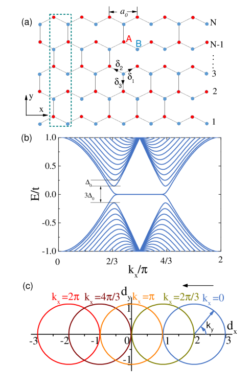
Figure 1: The surface states in graphene ribbon with zigzag edges. (a) Scheme of graphene ribbon with zigzag edges. $N$ is the number of zigzag lines. Here $a_{0}=\sqrt{3}a$. (b) The spectrum of graphene ribbon with zigzag edges. (c) The end point of vector $\hat{{\bf d}}({\bf k})$ forms unit circles as changing $k_{y}$. Here $k_{y}$ works as a polar angle.

We find it is more concise and straightforward to understand the surface states by identifying the graphene ribbon as an SSH model in the reduced 1D parameter space. SSH model describes spinless electrons sitting in a 1D dimer chain, and it has been extensively studied as a prototype for associated topological properties SSH79prl ; Shen2017 ; Asboth2015 . In the following we make a simple connection between the SSH model and graphene ribbons. Graphene has a honeycomb lattice structure as shown in Fig. 1(a). The three nearest-neighbor vectors in real space are denoted as $\bm{\delta}_{1}=\frac{a}{2}(\sqrt{3},1),\ \ \bm{\delta}_{2}=\frac{a}{2}(-\sqrt{3},1),\ \ \bm{\delta}_{3}=a(0,-1)$ with $a$ the carbon-carbon distance. Considering only nearest-neighbor hopping, the tight-binding Hamiltonian for electrons in graphene reads

$$H=t\sum_{\bm{R}_{B}}\sum_{\ell=1}^{3}C_{\bm{R}_{B}+\bm{\delta}_{\ell}}^{\dagger}C_{\bm{R}_{B}}+h.c.,$$ (1)

where $C_{\bm{R}}^{\dagger}$($C_{\bm{R}}$) creates (annihilates) an electron at site $\bm{R}$. Here the spin degree of freedom is suppressed and $t$ is the nearest-neighbor hopping energy. In the following, we first focus our attention on graphene ribbon with zigzag edges and then analyze ribbons with beared and armchair edges. After performing partial Fourier transformation in $x$ direction, the zigzag ribbon is reduced to 1D fictitious chain along $y$ direction, in which each unit cell contains two sites. The hopping energy in and between unit cells of the chain is different, i.e., $2t\cos(\sqrt{3}ak_{x}/2)$ for intracell hopping and $t$ for intercell hopping. Therefore, the reduced zigzag ribbon is identical to SSH model of dimerized 1D lattice. The spectrum of graphene ribbons with zigzag edges obtained in this way is shown in Fig. 1(b), in which the flat band surface states connect $K$ and $K^{\prime}$ valleys. Imposing periodic boundary condition along $y$ direction further, the system is described by the Hamiltonian

$$h_{k_{x}}^{Z}(k_{y})=[2\cos\frac{\sqrt{3}k_{x}a}{2}+\cos\frac{3k_{y}a}{2}]\sigma_{x}+\sin\frac{3k_{y}a}{2}\sigma_{y}\equiv\bm{d}(\bm{k})\cdot\mathbf{\bm{\sigma}},$$ (2)

where $\mathbf{\bm{\sigma}\equiv}(\sigma_{x},\sigma_{y})$ is the Pauli matrix vector, and $\bm{d}(\bm{k})=(2\cos(\sqrt{3}k_{x}a/2)+\cos(3k_{y}a/2),\sin(3k_{y}a/2))$. The wave numbers are normalized with corresponding primitive translation vectors, and the energy is scaled by hopping energy $t$. Note that the primitive lattice spacings in $x$ and $y$ directions are $\sqrt{3}a$ and $3a/2$, respectively. Diagonalizing the Hamiltonian of Eq. 2, we obtain the spectrum that is consistent with the very one of zigzag graphene Rhim18prb ; Waka99prb . It should be noted that Eq. 2 is exactly the SSH Hamiltonian if we redefine $d_{x}(k_{y})=v+w\cos k_{y}$ and $d_{y}(k_{y})=w\sin k_{y}$ with $v\equiv 2\cos(k_{x}/2)$ and $w\equiv 1$ Shen2017 ; Asboth2015 . The topology of SSH model is characterized by the winding number defined as $\bm{\nu}=\frac{1}{2\pi i}\oint q^{-1}dq$ with $q=v+we^{-ik_{y}}$. Since $\bm{\nu}=1$ for $|v|<|w|$ in SSH model, the zigzag graphene is topologically nontrivial with wave vector $k_{x}$ locating in the region $(\frac{2\pi}{3},\frac{4\pi}{3})$. From the bulk-boundary correspondence, there are surface states connecting $K$ and $K^{\prime}$ valleys, as shown in Fig. 1(b). For the region $k_{x}\in(0,\frac{2\pi}{3})\cup(\frac{4\pi}{3},2\pi)$, the winding number is zero and no surface states are expected. We can also interpret the topology of graphene ribbons in terms of the Zak phase Zak88prl , which gives consistent results as winding numbers.

The vector $\bm{d}(\bm{k})$ provides a more vivid way to explore the topology of Eq. 2. The path of the end point of vector $\bm{d}(\bm{k})$, as the wave number $k_{y}$ goes through the 1D Brillouin zone $[0,2\pi]$, is a unit circle centered at $\left(2\cos(k_{x}/2),0\right)$ on the $d_{x}$-$d_{y}$ plane, as shown in Fig. 1(c). Increasing $k_{x}$ moves the unit circle left. Once the circle cuts the origin, it gives Dirac cone. Varying the wave vector $k_{x}$ from $0$ to $2\pi$, the gap of the reduced 1D system will close at $k_{x}=2\pi/3$ then reopen, and similar process happens again around $k_{x}=4\pi/3$. This gap close-reopen process may indicate topological phase transition. Whether or not the system is topologically nontrivial is determined by the origin is enclosed by the unit circle or not. Similar analysis can also be applied to graphene ribbon with beared and armchair edges. For example, the reduced Hamiltonian for the beared edge case is $h_{k_{x}}^{B}(k_{y})=[1+2\cos(k_{x}/2)\cos k_{y}]\sigma_{x}+2\cos(k_{x}/2)\sin k_{y}\sigma_{y}.$ Following the same argument, there are flat band surface states in the region $k_{x}\in(0,\frac{2\pi}{3})\cup(\frac{4\pi}{3},2\pi)$. For the ribbons with armchair edges, there are no such surface states.

II.2 Constructing valley chiral bands by edge potentials

We demonstrated in the previous section that the surface states in the zigzag graphene ribbons can be interpreted by SSH model.In this section we show how to construct genuinely chiral bands using these surface states in order to realize pseudo chiral anomaly in graphene ribbon with zigzag edges.

The wave functions of surface states at $k_{x}=\pi$ with energy $E=0$ are entirely localized at the edges of the ribbon. Applying edge potentials $U_{\mathrm{edge}}$ at the outmost sites of two edges, intuitively, drags the surface states to the states with energy $E=U_{\mathrm{edge}}$ Yao12prl . Considering the band structures as shown in Fig. 1(b), in which the energies of all other bands coincide at $E=\pm 1$ for $k_{x}=\pi$, we choose the confining edge potentials to be $U_{\mathrm{edge}}=\pm 1$. For the case of $U_{\mathrm{edge}}=-1$, gapless chiral bands, labeled as $n=0$, cross the valleys, as seen in Fig. 2(a). Focusing on the left (right) valley, modes $n=1,2,\cdots,N$ lie above the $n=0$ chiral band, whereas modes $n=-1,-2,\cdots,-(N-1)$ lie below the $n=0$ chiral band, and the gapless chiral band cross the valley with group velocity $v_{F}=-\frac{3}{2}\frac{ta}{\hbar}$ ($v_{F}=+\frac{3}{2}\frac{ta}{\hbar}$). The two $n=0$ chiral bands should be stable, as will be shown, since they originate from the topologically protected surface states.

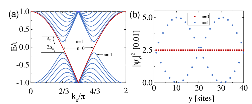
Figure 2: Constructing the gapless chiral bands by introducing edge potentials. (a) The spectrum of graphene ribbon with zigzag edges confined by edge potentials. The chiral bands are emphasized by red lines. (b) The wave function for $k_{x}=2\pi/3$ corresponding to panel (a).

The wave numbers $k_{x}=2\pi/3$ and $k_{x}=4\pi/3$ are unique points at which the system has special energy and wave functions. For $k_{x}=2\pi/3$ and $k_{x}=4\pi/3$, the Hamiltonian for the zigzag graphene ribbons confined by the edge potentials turns out to be

$$h_{\eta}^{Z}=\left(\begin{array}[]{ccccc}U_{\mathrm{edge}}&-\eta&\cdots&0&0\\ -\eta&0&\ddots&0&0\\ \vdots&\ddots&\ddots&\ddots&\vdots\\ \vdots&\vdots&-\eta&0&-\eta\\ 0&\cdots&0&-\eta&U_{\mathrm{edge}}\end{array}\right)$$ (3)

under the basis $(C_{\eta A1},C_{\eta B1},C_{\eta A2},C_{\eta B2},\cdots,C_{\eta AN},C_{\eta BN})^{T}$. Here $\eta=-1$ for $k_{x}=2\pi/3$ and $\eta=+1$ for $k_{x}=4\pi/3$, respectively. For $U_{\mathrm{edge}}=-1,$ the eigen values of Eq. 3 read

$$E_{\eta,j}=2\cos[j\pi/(2N)],\ \ \ j=1,2,...,2N.$$ (4)

The zero-energy modes, corresponding to the chiral bands $n=0$, always exist when $j=N$. By Taylor expansion and elimination of $N$ from the width $W=(3N/2-1)a$, the mode spacing under the limit $W\gg 1$ is

$$\Delta_{0}=3ta\pi/(2W),$$ (5)

which is proportional to $1/W$. The energy separation of the conduction and valence bands, as shown in Fig. 2(a), is $2\Delta_{0}$ now and different from $3\Delta_{0}$ as in Fig. 1(b) Rycerz07np . The corresponding eigenvectors for $n=0$ chiral bands are

$$\psi_{\eta}(y)=\frac{1}{\sqrt{2N}}(1,-\eta,-1,\eta,1,-\eta,\cdots)^{T}.$$ (6)

It is interesting to note from Fig. 2(b) that the wave functions of the $n=0$ chiral bands are not localized at edges but distribute equally on each site along $y$ direction (it is even true at $k_{x}\neq\eta$), which is different from the case where the bulk gap is opened Yao12prl .

III Results

III.1 Pseudo chiral anomaly in zigzag graphene ribbons

The spectrum in Fig. 2(a) is very similar to that of Weyl fermions in the presence of a strong magnetic field Hosur13phys , and it provides the possibility to realize chiral anomaly in graphene ribbons. Crucially, the chiral bands have definite chiralities just as the chiral Landau levels of Weyl fermions. Suppose the temperature is at zero and only the chiral bands are relevant, thus the system is in the so called ‘quantum limit’ regime. Applying an external electric field with strength $\bm{E}$ along the ribbon will drive electrons flowing from one valley to the other. The change rate of charge carrier density at one valley $\eta$($=\pm$) in the quasi-1D system is $\frac{d\rho_{\eta}}{dt}=\frac{\eta}{W}\frac{1}{2\pi}\frac{dk_{x}}{dt},$ and the momentum vector will obey the equation $\frac{dk_{x}}{dt}=\frac{e\bm{E}}{\hbar}$. Therefore, we have $\frac{d\rho_{\eta}}{dt}=\eta\frac{e}{h}\frac{\bm{E}}{W}$. Similar to chiral anomaly in Weyl semimetals, here we can also define an equation for divergence free current $j_{5}^{\mu}$ as

$$\partial_{\mu}j_{5}^{\mu}=\frac{\partial\rho_{+}}{\partial t}-\frac{\partial\rho_{-}}{\partial t}=\frac{2e}{h}\bm{E}\mathcal{B},$$ (7)

where $\mu=0,1$, $\partial_{0}\equiv\partial_{t}$ and $\partial_{1}\equiv\partial_{x}$, and $\mathcal{B}\equiv 1/W$. Physically, Eq. 7 states nonconservation of the chiral charge in the presence of electric field and effective magnetic field $\mathcal{B}$. Thus, by the same mechanism that is operative in 3D Weyl semimetals Nielsen83pl ; Pikulin16prx , the chiral anomaly can be generalized to quasi-1D graphene ribbons. Comparing with the current conservation equation of Weyl semimetals, $\mathcal{B}$ here takes the role of a magnetic field. This analogy also makes sense in terms of physical picture of Landau levels: In graphene ribbons, the energy band spacing $\Delta_{0}$ decreases with decreasing the effective magnetic field $\mathcal{B}$, i.e., $\Delta_{0}\propto\mathcal{B}$; and likewise the Landau level separation also decreases with decreasing the real magnetic field strength. It should be noted here we mainly focus on the orbital effect of a magnetic field imposed on electrons. The difference between the effective magnetic field $\mathcal{B}$ and a real magnetic field, however, lies in several aspects: First, the effective magnetic field $\mathcal{B}$ preserves time reversal symmetry; second, the unit of effective magnetic field $\mathcal{B}$ is not as well-defined as the real magnetic field; third, the effective magnetic field $\mathcal{B}$ has no Zeeman effect. For these reasons above, the chiral anomaly presented here in graphene ribbons is therefore referred to as pseudo chiral anomaly.

III.2 Transport signatures of the pseudo chiral anomaly

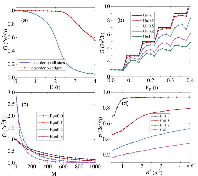
Figure 3: Transport of chiral bands under the effect of onsite disorders. (a) Conductance as functions of disorder strength $U$ with $E_{F}=0.01$, $M=34$ and $N=40$. (b) Conductance as functions of $E_{F}$ with $M=34$ and $N=40$. (c) Conductance as functions of length $M$ with $U=1$ and $N=20$. (d) The conductivity as function of effective magnetic field square $\mathcal{B}^{2}$ with $E_{F}=0.01$, and in this plot we take $N$ from 100 to 301. Here 5000 disorder configurations are taken for all.

Due to the interplay of chiral magnetic effect and intervalley scattering, the pseudo magnetoconductivity $\sigma(\mathcal{B})$ should be positive and have quadratic dependence on $\mathcal{B}$ in the diffusive transport regime LiC172D ; LiQ16npA , which is regarded as the signature of pseudo chiral anomaly in graphene. In this section, we try to reveal this anomalous scaling behavior of finite-size conductivity numerically. From Fig. 2(a), the left valley locates at $k_{-}=2\pi/3$ and the right valley locates at $k_{+}=4\pi/3$. The rather large momentum difference $\Delta k=2\pi/3$ between the two valleys indicates that the transport properties depend on impurity ranges heavily. As mentioned above, the signature of chiral anomaly will only be revealed with intervalley scattering. Thereby two typical kinds of disorders, namely, onsite disorders and Gaussian type disorders, are considered. The onsite disorders are considered by independently adding every lattice site a potential drawn from uniform distribution $[-U/2,U/2]$ with $U$ the disorder strength. For Gaussian type disorders uniformly distributed in the 2D real space, the potential on a lattice site with position $\bm{R}$ has the form Wakabayashi07prl

$$V(\bm{R})=\sum_{\bm{r}_{i}}u\exp(-|\bm{R}-\bm{r}_{i}|^{2}/d^{2}),$$ (8)

where $d$ is the disorder range and $\bm{r}_{i}$ is the disorder position. Here $u$ is the disorder strength uniformly distributed within $[-u_{m},u_{m}]$ constrained by the normalization condition

$$\sum_{\bm{R}\in\mathrm{full\ space}}u_{m}\exp(-|\bm{R}|^{2}/d^{2})/(\sqrt{3}/2)=u_{0}.$$ (9)

The Landau-B$\ddot{\mathrm{u}}$ttiker formalism provides an efficient way to calculate the transport properties of electrons. Here we consider a two-terminal setup with disordered central region connected to two clean leads. With the help of recursive Green’s function techniques, the conductance of two-terminal device can be evaluated as

$$G=\frac{2e^{2}}{h}Tr\left[\Gamma_{L}G^{r}\Gamma_{R}G^{a}\right],$$ (10)

where $\Gamma_{L,R}$ are the line-width functions coupling to left lead and right lead, respectively, and $G^{r}(G^{a})$ is the retarded (advanced) Green’s function of the disordered region Dattabook . Note that the conductivity meets $\sigma=G$ for a square sheet Tworzdlo06prl ; Lewenkopf08prb . Here the width $W=(3N/2-1)a$ and length $L=\sqrt{3}Ma$ with $M$ the number of defined unit cells in Fig. 1(a).

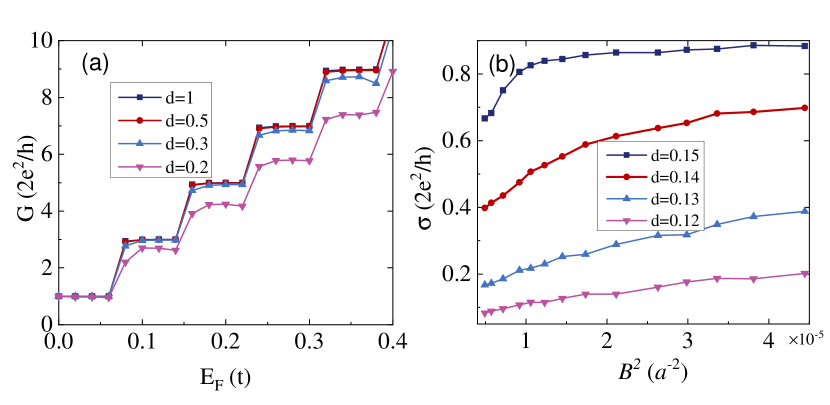
Figure 4: Transport of chiral bands under the effect of Gaussian type disorder. (a) Conductance as functions of $E_{F}$ with $M=34$ and $N=40$. (b) The conductivity as function of effective magnetic field square $\mathcal{B}^{2}$ with $E_{F}=0.01$, $u_{0}=1$. Here 5000 disorder configurations are taken for all.

Let us now consider the transport properties of the $n=0$ chiral bands. For a clean sample, the relevant chiral bands should underlie a quantized conductance $2e^{2}/h$. To verify the validity of chiral bands induced by edge potentials, the onsite disorders are added at the outmost sites of the two edges first. As seen in Fig. 3(a), the quantized conductance from chiral bands persists until edge disorder strength reaches critical strength $U_{c}\simeq 2.5$. Therefore, the mechanism of confining edge potentials still works as long as the disorder strength does not exceed the critical value $U_{c}$. While for the case where disorders are on all sites, the conductance decreases quickly as shown by blue line in Fig. 3(a). Seen from Fig. 3(b) (also in Fig. 4(a)), the $n=0$ chiral bands are more stable than other bands: The conductance plateau from $n=0$ chiral bands is nearly unchanged as increasing the disorder strength. The scaling behavior of conductance with respect to sample length also shows the robustness of the $n=0$ chiral bands (see Fig. 3(c)).

For onsite disorders, the pseudo magnetoconductivity as function of $\mathcal{B}^{2}$ with different disorder strengths is presented in Fig. 3(d): Focusing on the curve with disorder strength $U=1$, the conductivity drops from a constant value linearly with respect to $\mathcal{B}^{2}$ as soon as the system is in laterally diffusive regime where the width exceeds mean free path; with appropriate disorder strength, the pseudo magnetoconductivity has a nearly quadratic dependence on effective magnetic field $\mathcal{B}$ and it is treated as the transport signature of pseudo chiral anomaly. Here the Fermi energy shifts away from zero slightly to avoid strong fluctuations Adam07pnas , and we keep the assumption that the Fermi energy only crosses the two $n=0$ chiral bands. For Gaussian disorders, we fix the disorder strength at $u_{0}=1$ and vary the interacting range $d$. For a shorter interacting range $d$, the intervalley scattering is relatively stronger. It is shown from Fig. 4(b) that the pseudo magnetoconductivity shares similar behavior as in the onsite disorder case, i.e., it shows nearly quadratic scaling behavior on effective magnetic field $\mathcal{B}$. The mechanism for this ‘anomalous’ scaling feature is the joint effort of finite size confinement and chiral magnetic effect. The electron change rate is proportional to $1/W$ in the quasi-1D system, then small chemical potential difference induced from the balance between intervalley scattering and chiral magnetic effect also contains a factor $1/W$ LiC172D . Thus the current density is proportional to $1/W^{2}$. While note that the previous results show that the conductivity of graphene near the charge neutral point has weak dependence on size Lewenkopf08prb ; Cresti07prb , and it reaches at a minimal value at order of $e^{2}/h$ Tan07prl ; Terres16nc . Comparison of Fig. 3(d) and 4(b) indicates that transport properties of chiral bands exhibit little dependence on the disorder types but much on disorder strengths.

IV Discussion

Varying the termination direction away from zigzag case will gradually weak the pseudo chiral anomaly and finally it disappears at armchair case. Thus we mainly focus on zigzag type graphene ribbons, and it is mostly relevant for experiments. One possible concern about the analogy between graphene and Weyl semimetals is that the stability of graphene nodes, unlike Weyl nodes, needs to be protected by inversion symmetry BernevigBook . Consider staggered potentials $U_{A}=\Delta$ for $A$ sites and $U_{B}=-\Delta$ for $B$ sites universally in the graphene lattice. At this moment, the bulk bands are gaped with amount $2\Delta$. The winding number is not well-defined now due to the existence of mass term in the bulk Dirac Hamiltonian. However, there are still flat bands with energy $E=\pm\Delta$ Delplace11prb ; Yao12prl . After applying proper edge potentials, the chiral bands crossing two valleys persist as in Fig. 2(a), thereby the physics of pseudo chiral anomaly remains. Besides, the magnetic order at zigzag edges of graphene ribbons may have influence on the bulk states Fujita96jpsj . While the band gap opened by the magnetic order is negligible as long as the zigzag ribbons wider than 8 nanometers Magda14nature , which is satisfied in our considerations, i.e., $N=40\sim 300$ and $W=8.5\sim 64$ nm. Note the strong intervalley scattering can lead to Anderson localization. While generally the typical size scales regarding localization properties in 2D systems are very large, thus the 2D electron localization mechanism may have little influence on our quasi-1D system Fan14prb ; Bardarson07prl .

V Conclusions

In conclusion, we show that pseudo chiral anomaly may exist in graphene ribbon with zigzag edges. We first show that the zigzag graphene ribbon can be mapped to SSH model, and then we turn the flat band surface states of zigzag graphene ribbons to chiral bands, based on which the pseudo chiral anomaly can be realized. This pseudo chiral anomaly underlies anomalous scaling behavior of pseudo magnetoconductivity on the effective magnetic field $\mathcal{B}$. Further numerical calculations on the transport properties indicates the pseudo magnetoconductivity has a positive and nearly quadratic dependence on $\mathcal{B}$. This finding provides graphene as an alternative platform to explore the purely quantum chiral anomaly in solids.

- (1) A. H. Castro Neto, F. Guinea, N. M. R. Peres, K. S. Novoselov, and A. K. Geim, The electronic properties of graphene, Rev. Mod. Phys. 81, 109 (2009).
- (2) K. S. Novoselov, A. K. Geim, S. V. Morozov, D. Jiang, M. I. Katsnelson, I. V. Grigorieva, S. V. Dubonos, and A. A. Firsov, Two-dimensional gas of massless Dirac fermions in graphene, Nature 438, 197 (2005).
- (3) Y. Zhang, Y.-W. Tan, H. L. Stormer, and P. Kim, Experimental observation of the quantum Hall effect and Berry’s phase in graphene, Nature 438, 201 (2005).
- (4) Z. Jiang and Y. Zhang and Y.-W. Tan and H.L. Stormer, and P. Kim, Quantum Hall effect in graphene, Solid State Commun. 143, 14 (2007).
- (5) K. S. Novoselov, Z. Jiang, Y. Zhang, S. V. Morozov, H. L. Stormer, U. Zeitler, J. C. Maan, G. S. Boebinger, P. Kim, and A. K. Geim, Room-temperature quantum Hall effect in graphene, Science 315, 1379 (2007).
- (6) T. Ando, Y. Zheng, and H. Suzuura, Dynamical conductivity and zero-mode anomaly in honeycomb lattices, J. Phys. Soc. Jpn. 71, 1318 (2002).
- (7) J. Tworzydlo, B. Trauzettel, M. Titov, A. Rycerz, and C. W. J. Beenakker, Sub-Poissonian shot noise in graphene, Phys. Rev. Lett. 96, 246802 (2006).
- (8) Y.-W. Tan, Y. Zhang, K. Bolotin, Y. Zhao, S. Adam, E. H. Hwang, S. Das Sarma, H. L. Stormer, and P. Kim, Measurement of scattering rate and minimum conductivity in graphene, Phys. Rev. Lett. 99, 246803 (2007).
- (9) M. I. Katsnelson, K. S. Novoselov and A. K. Geim, Chiral tunneling and the Klein paradox in graphene, Nat. Phys. 2, 620 (2006).
- (10) N. Stander, B. Huard, and D. Goldhaber-Gordon, Evidence for Klein tunneling in graphene p-n junctions, Phys. Rev. Lett. 102, 026807 (2009).
- (11) P. Hosur and X. L. Qi, Recent developments in transport phenomena in Weyl semimetals, C. R. Phys. 14, 857 (2013).
- (12) N. P. Armitage, E. J. Mele, and A. Vishwanath, Weyl and Dirac semimetals in three-dimensional solids, Rev. Mod. Phys. 90, 015001 (2018).
- (13) X. Wan, A. M. Turner, A. Vishwanath, and S. Y. Savrasov, Topological semimetal and Fermi-arc surface states in the electronic structure of pyrochlore iridates, Phys. Rev. B 83, 205101 (2011).
- (14) S.-M. Huang, S.-Y. Xu, I. Belopolski, C.-C. Lee, G. Chang, B. Wang, N. Alidoust, G. Bian, M. Neupane, C. Zhang, S. Jia, A. Bansil, H. Lin, and M. Z. Hasan, A Weyl Fermion semimetal with surface Fermi arcs in the transition metal monopnictide TaAs class, Nat. Commun. 6, 7373 (2015).
- (15) S.-Y. Xu, I. Belopolski, N. Alidoust, M. Neupane, G. Bian, C. Zhang, R. Sankar, G. Chang, Z. Yuan, C.- C. Lee, S.-M. Huang, H. Zheng, J. Ma, D. S. Sanchez, B. Wang, A. Bansil, F. Chou, P. P. Shibayev, H. Lin, S. Jia, and M. Z. Hasan, Discovery of a Weyl fermion semimetal and topological Fermi arcs, Science 349, 613 (2015).
- (16) M. E. Peskin and D. V. Schroeder, An introduction to quantum field theory (Westview Press Inc., 1995).
- (17) H.-J. Kim, K.-S. Kim, J.-F. Wang, M. Sasaki, N. Satoh, A. Ohnishi, M. Kitaura, M. Yang, and L. Li, Dirac versus Weyl fermions in topological insulators: Adler-Bell-Jackiw anomaly in transport phenomena, Phys. Rev. Lett. 111, 246603 (2013).
- (18) X. Huang, L. Zhao, Y. Long, P. Wang, D. Chen, Z. Yang, H. Liang, M. Xue, H. Weng, Z. Fang, X. Dai, and G. Chen, Observation of the chiral-anomaly-induced negative magnetoresistance in 3D Weyl semimetal TaAs, Phys. Rev. X 5, 031023 (2015).
- (19) C.-Z. Li, L.-X. Wang, H. Liu, J. Wang, Z.-M. Liao, and D.-P. Yu, Giant negative magnetoresistance induced by the chiral anomaly in individual nanowires, Nat. Commun. 6, 10137 (2015).
- (20) H. Li, H. He, H.-Z. Lu, H. Zhang, H. Liu, R. Ma, Z. Fan, S.-Q. Shen, and J. Wang, Negative magnetoresistance in Dirac semimetal , Nat. Commun. 7, 10301 (2016).
- (21) S. Liang, J. Lin, S. Kushwaha, J. Xing, N. Ni, R. J. Cava, and N. P. Ong, Experimental tests of the chiral anomaly magnetoresistance in the Dirac-Weyl semimetals and GdPtBi, Phys. Rev. X 8, 031002 (2018).
- (22) S. A. Yang, Dirac and Weyl materials: fundamental aspects and some spintronics applications, SPIN 6, 1640003 (2016).
- (23) G. E. Volovik, The Universe in a Helium Droplet (Clarendon Press, 2003).
- (24) H. Nielsen and M. Ninomiya, Absence of neutrinos on a lattice: (I). Proof by homotopy theory, Nucl. Phys. B 185, 20 (1981).
- (25) H. Nielsen and M. Ninomiya, Absence of neutrinos on a lattice: (II). Intuitive topological proof, Nucl. Phys. B 193, 173 (1981).
- (26) S. Ryu and Y. Hatsugai, Topological origin of zero-energy edge states in particle-hole symmetric systems, Phys. Rev. Lett. 89, 077002 (2002).
- (27) S. L. Adler, Axial-vector vertex in spinor electrodynamics, Phys. Rev. 177, 2426 (1969).
- (28) J. S. Bell and R. Jackiw, A PCAC puzzle: in the -model, Nuovo Cimento A 60, 47 (1969).
- (29) H. Nielsen and M. Ninomiya, The Adler-Bell-Jackiw anomaly and Weyl fermions in a crystal, Phys. Lett. B 130, 389 (1983).
- (30) D. T. Son and B. Z. Spivak, Chiral anomaly and classical negative magnetoresistance of Weyl metals, Phys. Rev. B 88, 104412 (2013).
- (31) A. A. Burkov, Chiral anomaly and diffusive magnetotransport in Weyl metals, Phys. Rev. Lett. 113, 247203 (2014).
- (32) K. Fukushima, D. E. Kharzeev, and H. J. Warringa, Chiral magnetic effect, Phys. Rev. D 78, 074033 (2008).
- (33) Q. Li, D. E. Kharzeev, C. Zhang, Y. Huang, I. Pletikosic, A. V. Fedorov, R. D. Zhong, J. A. Schneeloch, G. D. Gu, and T. Valla,Chiral magnetic effect in , Nat. Phys. 12, 550 (2016).
- (34) J. Cai, P. Ruffieux, R. Jaafar, M. Bieri, T. Braun, S. Blankenburg, M. Muoth, A. P. Seitsonen, M. Saleh, X. Feng, K. Mullen, and R. Fasel, Atomically precise bottom-up fabrication of graphene nanoribbons, Nature 466, 470 (2010).
- (35) P. Ruffieux, S. Wang, B. Yang, C. Snchez-Snchez,J. Liu, T. Dienel, L. Talirz, P. Shinde, C. A. Pignedoli, D. Passerone, T. Dumslaff, X. Feng, K. Mllen, and R. Fasel, On-surface synthesis of graphene nanoribbons with zigzag edge topology, Nature 531, 489 (2016).
- (36) M. Y. Han, B. yilmaz, Y. Zhang, and P. Kim, Energy band-gap engineering of graphene nanoribbons, Phys. Rev. Lett. 98, 206805 (2007).
- (37) C. Tao, L. Jiao, O. V. Yazyev, Y.-C. Chen, J. Feng, X. Zhang, R. B. Capaz, J. M. Tour, A. Zettl, S. G. Louie, H. Dai, and M. F. Crommie, Spatially resolving edge states of chiral graphene nanoribbons, Nat. Phys. 7, 616 (2011).
- (38) S. Wang, L.Talirz, C. A. Pignedoli, X. Feng, K. Mllen, R. Fasel, and P. Ruffieux, Giant edge state splitting at atomically precise graphene zigzag edges, Nat. Commun. 7, 11507 (2016).
- (39) O. Grning, S. Wang, X. Yao, C. A. Pignedoli, G. Borin Barin, C. Daniels, A. Cupo, V. Meunier, X. Feng, A. Narita, K. Mllen, P. Ruffieux, and R. Fasel, Engineering of robust topological quantum phases in graphene nanoribbons, Nature 560, 209 (2018).
- (40) D. J. Rizzo, G. Veber, T. Cao, C. Bronner, T. Chen, F. Zhao, H. Rodriguez, S. G. Louie, M. F. Crommie, and F. R. Fischer, Topological band engineering of graphene nanoribbons, Nature 560, 204 (2018).
- (41) H.-Z. Lu, S.-B. Zhang, and S.-Q. Shen, High-field magnetoconductivity of topological semimetals with short-range potential, Phys. Rev. B 92, 045203 (2015).
- (42) S.-Q. Shen, C.-A. Li, and Q. Niu, Chiral anomaly and anomalous finite-size conductivity in graphene, 2D Mater. 4, 035014 (2017).
- (43) K. Nakada, M. Fujita, G. Dresselhaus, and M. S. Dresselhaus, Edge state in graphene ribbons: Nanometer size effect and edge shape dependence, Phys. Rev. B 54, 17954 (1996).
- (44) L. Brey and H. A. Fertig, Electronic states of graphene nanoribbons studied with the Dirac equation, Phys. Rev. B 73, 235411 (2006).
- (45) Y. Hatsugai, Topological aspect of graphene physics, J. Phys. Conf. Ser. 334, 012004 (2011).
- (46) P. Delplace, D. Ullmo, and G. Montambaux, Zak phase and the existence of edge states in graphene, Phys. Rev. B 84, 195452 (2011).
- (47) T. Cao, F. Zhao, and S. G. Louie, Topological phases in graphene nanoribbons: junction states, spin centers, and quantum spin chains, Phys. Rev. Lett. 119, 076401 (2017).
- (48) J.-W. Rhim, J. H. Bardarson, and R.-J. Slager, Unified bulk-boundary correspondence for band insulators, Phys. Rev. B 97, 115143 (2018).
- (49) W. P. Su, J. R. Schrieffer, and A. J. Heeger, Solitons in polyacetylene, Phys. Rev. Lett. 42, 1698 (1979).
- (50) S.-Q. Shen, Topological Insultaors: Dirac equation in condensed matter, 2nd ed. (Springer, Singapore, 2017).
- (51) J. K. Asbth, L. Oroszlny, and A. Plyi, A short course on topological insulators: band structure topology and edge states in one and two dimensions (Springer-Verlag, Berlin, 2015).
- (52) K. Wakabayashi, M. Fujita, H. Ajiki, and M. Sigrist, Electronic and magnetic properties of nanographite ribbons, Phys. Rev. B 59, 8271 (1999).
- (53) J. Zak, Berry’s phase for energy bands in solids, Phys. Rev. Lett. 62, 2747 (1989).
- (54) W. Yao, S. A. Yang, and Q. Niu, Edge states in graphene: From gapped flat-band to gapless chiral modes, Phys. Rev. Lett. 102, 096801 (2009).
- (55) A. Rycerz, J. Tworzydlo, and C. W. J. Beenakker, Valley filter and valley valve in graphene, Nat. Phys. 3, 172 (2007).
- (56) D. I. Pikulin, A. Chen, and M. Franz, Chiral anomaly from strain-induced gauge fields in Dirac and Weyl semimetals, Phys. Rev. X 6, 041021 (2016).
- (57) Q. Li and D. E. Kharzeev, Chiral magnetic effect in condensed matter systems, Nucl. Phys. A 956, 107 (2016).
- (58) K. Wakabayashi, Y. Takane, and M. Sigrist, Perfectly conducting channel and universality crossover in disordered graphene nanoribbons, Phys. Rev. Lett. 99, 036601 (2007).
- (59) S. Datta, Electronic Transport in Mesoscopic Systems (Cambridge University Press, 1995).
- (60) C. H. Lewenkopf, E. R. Mucciolo, and A. H. Castro Neto, Numerical studies of conductivity and Fano factor in disordered graphene, Phys. Rev. B 77, 081410 (2008).
- (61) S. Adam, E. H. Hwang, V. M. Galitski, and S. Das Sarma, A self-consistent theory for graphene transport, Proc. Natl. Acad. Sci. USA 104, 18392 (2007).
- (62) A. Cresti, G. Grosso, and G. P. Parravicini, Numerical study of electronic transport in gated graphene ribbons, Phys. Rev. B 76, 205433 (2007).
- (63) B. Terrs, L. A. Chizhova, F. Libisch, J. Peiro, D. Joger, S. Engels, A. Girschik, K. Watanabe, T. Taniguchi, S. V. Rotkin, J. Burgdrfer, and C. Stampfer, Size quantization of Dirac fermions in graphene constrictions, Nat. Commun. 7, 151528 (2016).
- (64) B. A. Bernevig and T. L. Hughes, Topological insulators and topological superconductors (Princeton University Press, NJ, 2013).
- (65) M. Fujita. K. Wakabayashi, K. Nakada and K. Kusakabe, Perculiar localized states at zigzag graphite edge, J. Phys. Soc. Jpn. 65, 1920 (1996).
- (66) G. Z. Magda, X. Jin, I. Hagymsi, P. Vancs, Z. Osvth, P. Nemes-Incze, C. Hwang, L. P. Bir, and L. Tapaszt, Room-temperature magnetic order on zigzag edges of narrow graphene nanoribbons, Nature 514, 608 (2014).
- (67) Z. Fan, A. Uppstu, and A. Harju, Anderson localization in two-dimensional graphene with short-range disorder: One-parameter scaling and finite-size effects, Phys. Rev. B 89, 245422 (2014).
- (68) J. H. Bardarson, J. Tworzydło, P. W. Brouwer, and C. W. J. Beenakker, One-Parameter Scaling at the Dirac Point in Graphene, Phys. Rev. Lett. 99, 106801 (2007).