Nested coordinate Bethe wavefunctions
from the Bethe/Gauge correspondence

Abstract.

In [1, 2], Nekrasov applied the Bethe/Gauge correspondence to derive the $\mathfrak{su}\,(2)$ XXX spin-chain coordinate Bethe wavefunction from the IR limit of a 2D $\mathcal{N}=(2,2)$ supersymmetric $A_{1}$ quiver gauge theory with an orbifold-type codimension-2 defect. Later, Bullimore, Kim and Lukowski implemented Nekrasov’s construction at the level of the UV $A_{1}$ quiver gauge theory, recovered his result, and obtained further extensions of the Bethe/Gauge correspondence [3]. In this work, we extend the construction of the defect to $A_{M}$ quiver gauge theories to obtain the $\mathfrak{su}\,(M+1)$ XXX spin-chain nested coordinate Bethe wavefunctions. The extension to XXZ spin-chain is straightforward. Further, we apply a Higgsing procedure to obtain more general $A_{M}$ quivers and the corresponding wavefunctions, and interpret this procedure (and the Hanany-Witten moves that it involves) on the spin-chain side in terms of Izergin-Korepin-type specializations (and re-assignments) of the parameters of the coordinate Bethe wavefunctions.

1. Introduction

In [4, 5], Nekrasov and Shatashvili proposed the Bethe/Gauge correspondence between the on-shell Bethe eigenstates of XXX (resp. XXZ) spin-chain Hamiltonians and the vacuum states of 2D $\mathcal{N}=(2,2)$ supersymmetric (resp. 3D $\mathcal{N}=2$) quiver gauge theories .

In [1, 2], Nekrasov introduced an orbifold-type codimension-2 defect in the IR limit of an $A_{1}$ quiver gauge theory on the gauge side of the correspondence, and obtained the coordinate Bethe wavefunction in the $\mathfrak{su}\,(2)$ XXX spin-$\frac{1}{2}$ chain on the Bethe side [6, 7] .

In [3], Bullimore, Kim and Lukowski implemented Nekrasov’s defect construction at the level of the UV A-twisted $\mathcal{N}=(2,2)$ supersymmetric $A_{1}$ quiver gauge theories on $S^{\,2}$, and used the localization formulae of [8, 9] to recover Nekrasov’s result, amongst other results that further extend the Bethe/Gauge correspondence.

In this work, we extend the construction of [3] to $A_{M}$ quiver gauge theories with orbifold-type codimension-2 defects to obtain $\mathfrak{su}(M+1)$ XXX spin-chain nested coordinate Bethe wavefunctions, with spin states in the fundamental representation.

Further, we apply a Higgsing procedure to obtain more general $A_{M}$ quiver gauge theories with codimension-2 defects, and their corresponding nested coordinate Bethe wavefunctions, and interpret these generalizations on the spin-chain side (and the Hanany-Witten moves that they involve) as Izergin-Korepin-type specializations (and re-assignments of the roles) of the parameters. While we focus on results in XXX spin-chains, we outline their straightforward extension to XXZ spin-chains.

1.1. Outline of contents

In Section 2, we recall the localization formulae of Closset, Cremonesi and Park, for 2D $\mathcal{N}=(2,2)$ quiver gauge theories on $S^{\,2}$ [8] (and that of Benini and Zaffaroni, for $\mathcal{N}=2$ quiver gauge theories on $S^{\,2}\times S^{\,1}$ [9]), used in [3] to construct Nekrasov’s orbifold defect in 2D $A_{1}$ quiver gauge theory. Generalizing the discussion in [3] for $A_{1}$ quiver gauge theory, we formally introduce the equivariant characters and reconstruct the localization formulae in [8, 9] from them.

In Section 3, we recall the Bethe/Gauge correspondence [4, 5] for $A_{M}$ linear quiver gauge theories, and provide the equivariant characters for them.

In Section 4, after briefly recalling the construction of orbifold defects in $A_{1}$ quiver gauge theory, we extend this construction to a simple $A_{M}$ linear quiver gauge theory and obtain the nested coordinate Bethe wavefunctions of the $\mathfrak{su}(M+1)$ XXX spin-chain with spin states in the fundamental representation.

In Section 5, using a Higgsing procedure, we generalize the orbifold construction of Section 4 to more general $A_{M}$ linear quiver gauge theories and find the corresponding partition functions (as specializations of coordinate Bethe wavefunctions) of the corresponding $\mathfrak{su}(M+1)$ vertex lattice models. In Section 6, we interpret the Higgsing procedure as an Izergin-Korepin-type specialization of the lattice parameters on the Bethe side of the Bethe/Gauge correspondence, and interpret the Hanany-Witten moves that are involved in the Higgsing on the gauge side as a re-assignment of the lattice parameters on the Bethe side, and in Section 7, we include remarks.

In Appendix A, we discuss the partial domain wall partition functions (DWPFs) in the rational $\mathfrak{su}(2)$ (six-)vertex model and prove Proposition 4.5, and in Appendix B, we define the partition function of the $\mathfrak{su}(M+1)$ vertex model which corresponds to the orbifold defect in the $A_{M}$ quiver constructed in the present work.

2. Rewriting the localization formulae

We review the localization formulae of the partition functions of the A-twisted gauged linear sigma models (GLSMs) [10, 11], which are 2D A-twisted $\mathcal{N}=(2,2)$ supersymmetric gauge theories on the $\Omega$-deformed $S_{\hbar}^{\,2}$ [8] (and 3D twisted $\mathcal{N}=2$ gauge theories on $S_{\hbar}^{\,2}\times S^{\,1}$ [9]), where $\hbar$ is the $\Omega$-deformation parameter. Following [3], we provide the localization formulae in terms of equivariant characters which are more fundamental objects than the partition functions. The equivariant characters are used to construct orbifold defects in Sections 4 and 5.

2.1. Equivariant characters

Consider the 2D $\mathcal{N}=(2,2)$ (or 3D $\mathcal{N}=2$) supersymmetric gauge theory consisting of a vector multiplet $V$ in a Lie algebra $\mathfrak{g}$, of gauge group $G$, and $L$ chiral matter multiplets $\Phi_{\mathfrak{R}_{i}}^{r_{i}}$, with representations $\mathfrak{R}_{i}$ of $\mathfrak{g}$, $U(1)$ vector $R$-charges $r_{i}$ and twisted masses $\lambda_{i}$, $i=1,\ldots,L$. In the present work, $r_{i}=0$ or $2$. The vector multiplet $V$ contains scalars $\boldsymbol{u}=\{u_{1},\ldots,u_{\mathrm{rk}(\mathfrak{g})}\}$, which take values in $\mathfrak{h}\otimes_{\mathbb{R}}{\mathbb{C}}$ and parametrize the Coulomb branch of the gauge theory, where $\mathrm{rk}(\mathfrak{g})$ is the rank of $\mathfrak{g}$ and $\mathfrak{h}$ is the Cartan subalgebra of $\mathfrak{g}$.

Definition 2.1.

The equivariant characters of the vector multiplet $V$ and the chiral matter multiplet $\Phi_{\mathfrak{R}}^{r}$ are

(2.1) $$\chi_{\hbar}^{V}(\boldsymbol{u}):=-\sum_{\alpha\in\Delta_{+}}\frac{\mathrm{e}^{\,\alpha(\boldsymbol{u})}+\mathrm{e}^{-\alpha(\boldsymbol{u})}}{1-\mathrm{e}^{\,\hbar}},\qquad\chi_{\hbar}^{\Phi_{\,\mathfrak{R}}^{\,r}}(\boldsymbol{u}):=\sum_{\rho\in\mathfrak{R}}\frac{\mathrm{e}^{\,\rho(\boldsymbol{u})+\,\lambda+\,\hbar\,\delta_{\,r,\,2}}}{1-\mathrm{e}^{\,\hbar}},$$

where $\Delta_{+}$ is the set of positive roots of $\mathfrak{g}$, while $\alpha(\boldsymbol{u})$ and $\rho(\boldsymbol{u})$ are the canonical pairings. The equivariant characters charged with GNO charges $\boldsymbol{d}=\{d_{1},\ldots,d_{\,\mathrm{rk}(\mathfrak{g})}\}$, $d_{a}\in\pi_{1}(U(1))\cong{\mathbb{Z}}$, associated with the quantized magnetic fluxes of the $U(1)^{\,\mathrm{rk}(\mathfrak{g})}$ gauge fields on $S_{\hbar}^{\,2}$, are

(2.2) $$\chi_{\hbar,\boldsymbol{d}}^{P}(\boldsymbol{u}):=\chi_{+\hbar}^{P}(\boldsymbol{u}|_{+})+\chi_{-\hbar}^{P}(\boldsymbol{u}|_{-}),$$

where $P=V$ or $\Phi_{\mathfrak{R}}^{r}$, and

(2.3) $$u_{a}|_{\pm}=u_{a}\mp\frac{d_{a}}{2}\,\hbar$$

where the characters $\chi_{+\hbar}^{P}(\boldsymbol{u}|_{+})$ and $\chi_{-\hbar}^{P}(\boldsymbol{u}|_{-})$ are defined on the north pole and the south pole of $S_{\hbar}^{\,2}$, respectively.

Definition 2.2.

The total equivariant character is

(2.4) $$\chi_{\hbar}^{\mathrm{total}}(\boldsymbol{u}):=\chi_{\hbar}^{V}(\boldsymbol{u})+\sum_{i=1}^{L}\chi_{\hbar}^{\Phi_{\mathfrak{R}_{i}}^{r_{i}}}(\boldsymbol{u}),$$

and the total equivariant character with charges $\boldsymbol{d}$ is

(2.5) $$\chi_{\hbar,\boldsymbol{d}}^{\mathrm{total}}(\boldsymbol{u}):=\chi_{+\hbar}^{\mathrm{total}}(\boldsymbol{u}|_{+})+\chi_{-\hbar}^{\mathrm{total}}(\boldsymbol{u}|_{-})=\chi_{\hbar,\boldsymbol{d}}^{V}(\boldsymbol{u})+\sum_{i=1}^{L}\chi_{\hbar,\boldsymbol{d}}^{\Phi_{\mathfrak{R}_{i}}^{r_{i}}}(\boldsymbol{u})$$

2.2. Partition functions

Each character $\chi_{\hbar,\boldsymbol{d}}^{P}(\boldsymbol{u})$ with charges $\boldsymbol{d}$ can be expanded as

(2.6) $$\chi_{\hbar,\boldsymbol{d}}^{P}(\boldsymbol{u})=\sum_{I}\mathrm{e}^{w_{I}(\boldsymbol{u};\boldsymbol{d};\hbar)}-\sum_{J}\mathrm{e}^{v_{J}(\boldsymbol{u};\boldsymbol{d};\hbar)},$$

where (2.6) defines $w_{\,I}$ and $v_{\,J}$, and we obtain the building blocks of the topologically twisted partition functions of 2D and 3D gauge theories by

(2.7) $$\widehat{\mathcal{Z}}_{\boldsymbol{d}}^{P}(\boldsymbol{u};\hbar)=\frac{\prod_{J}v_{J}(\boldsymbol{u};\boldsymbol{d};\hbar)}{\prod_{I}w_{I}(\boldsymbol{u};\boldsymbol{d};\hbar)},$$

and

(2.8) $$\widehat{\mathcal{Z}}_{\boldsymbol{d}}^{\mathrm{K},P}(\boldsymbol{u};\hbar)=\frac{\prod_{J}2\sinh\left\lgroup v_{J}(\boldsymbol{u};\boldsymbol{d};\hbar)/2\right\rgroup}{\prod_{I}2\sinh\left\lgroup w_{I}(\boldsymbol{u};\boldsymbol{d};\hbar)/2\right\rgroup},$$

respectively.

Proposition 2.3.

The partition functions (2.7) and (2.8), which are obtained from Definition 2.1, as

(2.9) $$\begin{split}&\widehat{\mathcal{Z}}_{\boldsymbol{d}}^{V}(\boldsymbol{u};\hbar)=(-1)^{\sum_{\alpha\in\Delta_{+}}\left\lgroup\alpha(\boldsymbol{d})+1\right\rgroup}\,\prod_{\alpha\in\Delta_{+}}\left\lgroup\alpha(\boldsymbol{u})^{\,2}-\frac{\alpha(\boldsymbol{d})^{\,2}}{4}\,\hbar^{\,2}\right\rgroup,\\ &\widehat{\mathcal{Z}}_{\boldsymbol{d}}^{\Phi_{\mathfrak{R}}^{r}}(\boldsymbol{u};\hbar)=\prod_{\rho\in\mathfrak{R}}\frac{\hbar^{r-\rho(\boldsymbol{d})-1}}{\left\lgroup\frac{\rho(\boldsymbol{u})+\lambda}{\hbar}+\frac{r-\rho(\boldsymbol{d})}{2}\right\rgroup_{\rho(\boldsymbol{d})+1-r}},\end{split}$$

and

(2.10) $$\begin{split}&\widehat{\mathcal{Z}}_{\boldsymbol{d}}^{\mathrm{K},V}(\boldsymbol{u};\hbar)=\left\lgroup-q^{-\frac{1}{2}}\right\rgroup^{\sum_{\alpha\in\Delta_{+}}\alpha(\boldsymbol{d})}\,\prod_{\alpha\in\Delta_{+}}\left\lgroup 1-\boldsymbol{u}^{-\alpha}q^{\frac{1}{2}\alpha(\boldsymbol{d})}\right\rgroup\left\lgroup 1-\boldsymbol{u}^{\alpha}q^{\frac{1}{2}\alpha(\boldsymbol{d})}\right\rgroup,\\ &\widehat{\mathcal{Z}}_{\boldsymbol{d}}^{\mathrm{K},\Phi_{\mathfrak{R}}^{r}}(\boldsymbol{u};\hbar)=\prod_{\rho\in\mathfrak{R}}\frac{\left\lgroup\boldsymbol{u}^{\rho}\Lambda\right\rgroup^{\frac{\rho(\boldsymbol{d})+1-r}{2}}}{\left\lgroup\boldsymbol{u}^{\rho}\Lambda q^{\frac{r-\rho(\boldsymbol{d})}{2}};q\right\rgroup_{\rho(\boldsymbol{d})+1-r}},\end{split}$$

respectively, give the building blocks of 2D and 3D topologically twisted partition functions in [8, 9] (see Proposition 2.4). Here $U_{a}=\mathrm{e}^{-u_{a}}$, $\Lambda=\mathrm{e}^{-\lambda}$, $q=\mathrm{e}^{-\hbar}$, $\boldsymbol{u}^{\alpha}=\mathrm{e}^{-\alpha(\boldsymbol{u})}$, and $\boldsymbol{u}^{\rho}=\mathrm{e}^{-\rho(\boldsymbol{u})}$.

In the above proposition, the Pochhammer and $q$-Pochhammer symbols are, respectively, defined by

(2.11) $$\begin{split}(x)_{d}=\frac{\Gamma(x+d)}{\Gamma(x)}=\begin{cases}\prod_{\ell=0}^{d}\left\lgroup x+\ell\right\rgroup\ \ &\textrm{if}\ d>0,\\ 1&\textrm{if}\ d=0,\\ \prod_{\ell=d}^{-1}\left\lgroup x+\ell\right\rgroup^{-1}\ \ &\textrm{if}\ d<0,\end{cases}\end{split}$$

and

(2.12) $$\begin{split}(x;q)_{d}=\begin{cases}\prod_{\ell=0}^{d}\left\lgroup 1-xq^{\ell}\right\rgroup\ \ &\textrm{if}\ d>0,\\ 1&\textrm{if}\ d=0,\\ \prod_{\ell=d}^{-1}\left\lgroup 1-xq^{\ell}\right\rgroup^{-1}\ \ &\textrm{if}\ d<0\end{cases}\end{split}$$

In the following, we assume that the gauge group $G$ contains central $U(1)^{\mathsf{c}}$ factors, and then one can deform the gauge theory by the associated Fayet-Iliopoulos (FI) parameters $\xi^{\,a}$, and theta angles $\theta^{\,a}$, $a=1,\ldots,\mathsf{c}$.

Proposition 2.4 ([8, 9]).

Combining the complexified FI parameters $\tau^{\,a}=\mathrm{i}\,\xi^{\,a}+\frac{1}{2\pi}\,\theta^{\,a}$ with the building blocks in Proposition 2.3 obtained from (2.5), up to sign factors, the partition function of the A-twisted GLSM on $S_{\hbar}^{\,2}$ is given by

(2.13) $$Z_{S_{\hbar}^{\,2}}=\frac{1}{|\mathcal{W}|}\sum_{\boldsymbol{d}\in{\mathbb{Z}}^{\mathrm{rk}(\mathfrak{g})}}\oint_{\Gamma}d^{\mathrm{rk}(\mathfrak{g})}u\,\widehat{\mathcal{Z}}_{\boldsymbol{d}}^{\textrm{total}}(\boldsymbol{u};\hbar),$$

where

(2.14) $$\widehat{\mathcal{Z}}_{\boldsymbol{d}}^{\textrm{total}}(\boldsymbol{u};\hbar):=\mathrm{e}^{2\pi\mathrm{i}\,\tau(\boldsymbol{d})}\,\widehat{\mathcal{Z}}_{\boldsymbol{d}}^{V}(\boldsymbol{u};\hbar)\,\prod_{i=1}^{L}\widehat{\mathcal{Z}}_{\boldsymbol{d}}^{\Phi_{\mathfrak{R}_{i}}^{r_{i}}}(\boldsymbol{u};\hbar)$$

Here $|\mathcal{W}|$ is the order of the Weyl group of $G$, and the pairing $\tau(\boldsymbol{d})=\sum_{a}\tau^{\,a}d_{a}$ is defined by embedding ${\boldsymbol{\tau}}$ into $\mathfrak{h}^{*}\otimes_{\mathbb{R}}{\mathbb{C}}$. The contour integral along $\Gamma$ is given by the Jeffrey-Kirwan residue operation (JK contour integral) [12, 13, 14] (see also [15]), which picks relevant poles of the integrand. Similarly, the correlation function of two codimension-2 defects, $\mathcal{O}_{N}(\boldsymbol{u})$ and $\mathcal{O}_{S}(\boldsymbol{u})$, inserted at the north pole and at the south pole of $S_{\hbar}^{\,2}$, respectively, is given by

(2.15) $$\left<\mathcal{O}_{N}(\boldsymbol{u})\,\mathcal{O}_{S}(\boldsymbol{u})\right>_{S_{\hbar}^{\,2}}=\frac{1}{|\mathcal{W}|}\sum_{\boldsymbol{d}\in{\mathbb{Z}}^{\mathrm{rk}(\mathfrak{g})}}\oint_{\Gamma}d^{\mathrm{rk}(\mathfrak{g})}u\,\widehat{\mathcal{Z}}_{\boldsymbol{d}}^{\textrm{total}}(\boldsymbol{u};\hbar)\,\mathcal{O}_{N}(\boldsymbol{u}|_{+})\,\mathcal{O}_{S}(\boldsymbol{u}|_{-})$$

The topologically twisted partition function and correlation functions of the $\mathcal{N}=2$ gauge theory on $S_{\hbar}^{\,2}\times S^{\,1}$ are obtained, up to Chern-Simons factors, by replacing $\widehat{\mathcal{Z}}_{\boldsymbol{d}}^{P}(\boldsymbol{u};\hbar)$ with $\widehat{\mathcal{Z}}_{\boldsymbol{d}}^{\mathrm{K},P}(\boldsymbol{u};\hbar)$ in the above formulae.

3. The Bethe/Gauge correspondence

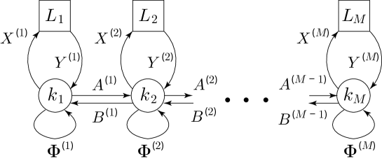
Figure 1. $A_{M}$ linear quiver with the matter content in Table 1.

We recall the basics of the Bethe/Gauge correspondence [4, 5], between the supersymmetric vacua of 2D $\mathcal{N}=(2,2)$ (resp. 3D $\mathcal{N}=2$) $A_{M}$ linear quiver gauge theories as in Figure 1, and the Bethe eigenfunctions of XXX (resp. XXZ) spin-chain Hamiltonians, with spins in the fundamental representation of $\mathfrak{su}(M+1)$.

Field	$U(k_{p})$	$U(k_{p+1})$	$U(k_{q})$	twisted mass	$U(1)_{R}$
$X_{i}^{(p)}$	$\mathbf{k}_{p}$	$\mathbf{1}$	$\mathbf{1}$	$-m_{i}^{(p)}-\frac{\gamma}{2}$	$0$
$Y_{i}^{(p)}$	$\overline{\mathbf{k}}_{p}$	$\mathbf{1}$	$\mathbf{1}$	$m_{i}^{(p)}-\frac{\gamma}{2}$	$0$
$\Phi^{(p)}$	adj	$\mathbf{1}$	$\mathbf{1}$	$\gamma$	$2$
$A^{(p)}$	$\mathbf{k}_{p}$	$\overline{\mathbf{k}}_{p+1}$	$\mathbf{1}$	$-\frac{\gamma}{2}$	$0$
$B^{(p)}$	$\overline{\mathbf{k}}_{p}$	$\mathbf{k}_{p+1}$	$\mathbf{1}$	$-\frac{\gamma}{2}$	$0$

Table 1. The matter content of the $A_{M}$ quiver gauge theory in Figure 1 which describes an $\mathfrak{su}(M+1)$ spin-chain. For $X_{i}^{(p)}$, $Y_{i}^{(p)}$, $\Phi^{(p)}$, $i=1,\ldots,L_{\,p}$ and $p=1,\ldots,M$. For $A^{(p)}$, $B^{(p)}$, $p=1,\ldots,M-1$. Further, $q=1,\ldots,M$, with $q\neq p,p+1$, and $U(1)_{R}$ denotes the $U(1)$ vector $R$-charge.

The $A_{M}$ quiver gauge theory which corresponds to the $\mathfrak{su}(M+1)$ XXX spin-chain, with spins in the fundamental representation, is described by an A-twisted GLSM, on the $\Omega$-deformed $S_{\hbar}^{\,2}$, with the gauge group $U(k_{1})\times\cdots\times U(k_{M})$, the matter content in Table 1, and the superpotential

$$W=\sum_{p=1}^{M}\sum_{i=1}^{L_{\,p}}\sum_{a,b=1}^{k_{\,p}}X_{i,a}^{(p)}\,\Phi_{a,b}^{(p)}\,Y_{b,i}^{(p)}+\sum_{p=1}^{M-1}\sum_{a,b=1}^{k_{\,p}}\sum_{c=1}^{k_{p+1}}\Phi_{a,b}^{(p)}\,A_{b,c}^{(p)}\,B_{c,a}^{(p)}+\sum_{p=1}^{M-1}\sum_{a=1}^{k_{\,p}}\sum_{b,c=1}^{k_{p+1}}A_{a,b}^{(p)}\,\Phi_{b,c}^{(p+1)}\,B_{c,a}^{(p)}$$

It contains a set of vector multiplet scalars $\boldsymbol{u}_{\boldsymbol{k}}^{M}=\{\boldsymbol{u}_{k_{1}}^{(1)},\ldots,\boldsymbol{u}_{k_{M}}^{(M)}\}$, with $\boldsymbol{u}_{k_{\,p}}^{(p)}=\{u_{1}^{(p)},\ldots,u_{k_{\,p}}^{(p)}\}$, which parametrize the Coulomb branch, and twisted masses $\boldsymbol{m}_{\boldsymbol{L}}^{M}=\{\boldsymbol{m}_{L_{1}}^{(1)},$ $\ldots,\boldsymbol{m}_{L_{M}}^{(M)}\}$, with $\boldsymbol{m}_{L_{\,p}}^{(p)}=\{m_{1}^{(p)},\ldots,m_{L_{\,p}}^{(p)}\}$ and $\gamma$, associated with the $U(L_{1})\times\cdots\times U(L_{M})\times U(1)$ flavor symmetry. In Table 2, we summarize the Bethe/Gauge dictionary [4, 5] which translates the gauge theory language to the spin-chain language. From Definition 2.1, we obtain the equivariant characters for the $U(k_{\,p})$ vector multiplets $V^{(p)}$ and the chiral matter multiplets in Table 1 as

(3.1) $$\begin{split}&\chi_{\hbar}^{V^{(p)}}\left\lgroup\boldsymbol{u}_{k_{\,p}}^{(p)}\right\rgroup=-\sum_{a\neq b}^{k_{\,p}}\frac{\mathrm{e}^{u_{a,b}^{(p)}}}{1-\mathrm{e}^{\hbar}},\qquad\chi_{\hbar}^{\Phi^{(p)}}\left\lgroup\boldsymbol{u}_{k_{\,p}}^{(p)}\right\rgroup=\sum_{a,b=1}^{k_{\,p}}\frac{\mathrm{e}^{u_{a,b}^{(p)}+\gamma+\hbar}}{1-\mathrm{e}^{\hbar}},\\ &\chi_{\hbar}^{X_{i}^{(p)}}\left\lgroup\boldsymbol{u}_{k_{\,p}}^{(p)}\right\rgroup=\sum_{a=1}^{k_{\,p}}\frac{\mathrm{e}^{u_{a}^{(p)}-m_{i}^{(p)}-\frac{\gamma}{2}}}{1-\mathrm{e}^{\hbar}},\qquad\chi_{\hbar}^{Y_{i}^{(p)}}\left\lgroup\boldsymbol{u}_{k_{\,p}}^{(p)}\right\rgroup=\sum_{a=1}^{k_{\,p}}\frac{\mathrm{e}^{-u_{a}^{(p)}+m_{i}^{(p)}-\frac{\gamma}{2}}}{1-\mathrm{e}^{\hbar}},\\ &\chi_{\hbar}^{A^{(p)}}\left\lgroup\boldsymbol{u}_{k_{\,p}}^{(p)},\boldsymbol{u}_{k_{p+1}}^{(p+1)}\right\rgroup=\sum_{a=1}^{k_{\,p}}\sum_{b=1}^{k_{p+1}}\frac{\mathrm{e}^{u_{a}^{(p)}-u_{b}^{(p+1)}-\frac{\gamma}{2}}}{1-\mathrm{e}^{\hbar}},\\ &\chi_{\hbar}^{B^{(p)}}\left\lgroup\boldsymbol{u}_{k_{\,p}}^{(p)},\boldsymbol{u}_{k_{p+1}}^{(p+1)}\right\rgroup=\sum_{a=1}^{k_{\,p}}\sum_{b=1}^{k_{p+1}}\frac{\mathrm{e}^{-u_{a}^{(p)}+u_{b}^{(p+1)}-\frac{\gamma}{2}}}{1-\mathrm{e}^{\hbar}},\end{split}$$

where $u_{a,b}^{(p)}=u_{a}^{(p)}-u_{b}^{(p)}$.

	2D/3D gauge with $A_{M}$ quiver (Figure 1)	$\mathfrak{su}(M+1)$ XXX/XXZ spin-chain
$u_{a}^{(p)}$	vector multiplet scalar	Bethe root
$m_{i}^{(p)}$	twisted mass	inhomogeneity
$\gamma$	twisted mass	coupling constant
$\mathfrak{q}_{p}$	exponentiated FI parameter	periodic spin-chain boundary twist parameter
(3.7)	effective twisted superpotential	Yang-Yang function
(3.8)	vacuum equation	nested Bethe equation

Table 2. The Bethe/Gauge dictionary, where $a=1,\ldots,k_{\,p}$, $i=1,\ldots,L_{\,p}$, $p=1,\ldots,M$. Here $k_{\,p}$ is the number of vector multiplet scalars in $U(k_{\,p})$ on the gauge side/spin excitations on the Bethe side, and $L_{\,p}$ is the number of (anti-)fundamental flavors in $U(k_{\,p})$ on the gauge side/total number of spins on the Bethe side.

Then, the building blocks of the $S^{\,2}$ partition function in Proposition 2.3 are obtained as

(3.2) $$\begin{split}&\widehat{\mathcal{Z}}_{\boldsymbol{d}_{k_{\,p}}^{(p)}}^{V^{(p)}}\left\lgroup\boldsymbol{u}_{k_{\,p}}^{(p)};\hbar\right\rgroup=(-1)^{(k_{\,p}-1)\sum_{a=1}^{k_{\,p}}(d_{a}^{(p)}+\frac{1}{2})}\prod_{a<b}^{k_{\,p}}\left\lgroup(u_{a,b}^{(p)})^{\,2}-\frac{(d_{a,b}^{(p)})^{\,2}}{4}\,\hbar^{\,2}\right\rgroup,\\ &\widehat{\mathcal{Z}}_{\boldsymbol{d}_{k_{\,p}}^{(p)}}^{\Phi^{(p)}}\left\lgroup\boldsymbol{u}_{k_{\,p}}^{(p)};\hbar\right\rgroup=\prod_{a,b=1}^{k_{\,p}}\mathcal{Z}^{(d_{a,b}^{(p)}-2)}\left\lgroup u_{a,b}^{(p)}+\gamma\right\rgroup,\\ &\widehat{\mathcal{Z}}_{\boldsymbol{d}_{k_{\,p}}^{(p)}}^{X_{i}^{(p)}}\left\lgroup\boldsymbol{u}_{k_{\,p}}^{(p)};\hbar\right\rgroup=\prod_{a=1}^{k_{\,p}}\mathcal{Z}^{(d_{a}^{(p)})}\left\lgroup u_{a}^{(p)}-m_{i}^{(p)}-\frac{\gamma}{2}\right\rgroup,\\ &\widehat{\mathcal{Z}}_{\boldsymbol{d}_{k_{\,p}}^{(p)}}^{Y_{i}^{(p)}}\left\lgroup\boldsymbol{u}_{k_{\,p}}^{(p)};\hbar\right\rgroup=\prod_{a=1}^{k_{\,p}}\mathcal{Z}^{(-d_{a}^{(p)})}\left\lgroup-u_{a}^{(p)}+m_{i}^{(p)}-\frac{\gamma}{2}\right\rgroup,\\ &\widehat{\mathcal{Z}}_{\boldsymbol{d}_{k_{\,p}}^{(p)},\boldsymbol{d}_{k_{p+1}}^{(p+1)}}^{A^{(p)}}\left\lgroup\boldsymbol{u}_{k_{\,p}}^{(p)},\boldsymbol{u}_{k_{p+1}}^{(p+1)};\hbar\right\rgroup=\prod_{a=1}^{k_{\,p}}\prod_{b=1}^{k_{p+1}}\mathcal{Z}^{(d_{a}^{(p)}-d_{b}^{(p+1)})}\left\lgroup u_{a}^{(p)}-u_{b}^{(p+1)}-\frac{\gamma}{2}\right\rgroup,\\ &\widehat{\mathcal{Z}}_{\boldsymbol{d}_{k_{\,p}}^{(p)},\boldsymbol{d}_{k_{p+1}}^{(p+1)}}^{B^{(p)}}\left\lgroup\boldsymbol{u}_{k_{\,p}}^{(p)},\boldsymbol{u}_{k_{p+1}}^{(p+1)};\hbar\right\rgroup=\prod_{a=1}^{k_{\,p}}\prod_{b=1}^{k_{p+1}}\mathcal{Z}^{(-d_{a}^{(p)}+d_{b}^{(p+1)})}\left\lgroup-u_{a}^{(p)}+u_{b}^{(p+1)}-\frac{\gamma}{2}\right\rgroup,\end{split}$$

where $\boldsymbol{d}_{\boldsymbol{k}}^{M}=\{\boldsymbol{d}_{k_{1}}^{(1)},\ldots,\boldsymbol{d}_{k_{M}}^{(M)}\}$ with $\boldsymbol{d}_{k_{\,p}}^{(p)}=\{d_{1}^{(p)},\ldots,d_{k_{\,p}}^{(p)}\}$, $d_{a}^{(p)}\in{\mathbb{Z}}$, $p=1,\ldots,M$, are sets of GNO charges, $d_{a,b}^{(p)}=d_{a}^{(p)}-d_{b}^{(p)}$, and

(3.3) $$\mathcal{Z}^{(d)}(u)=\begin{cases}\prod_{\ell=0}^{d}\left\lgroup u-\frac{d}{2}\,\hbar+\ell\,\hbar\right\rgroup^{-1}\ \ &\textrm{if}\ d\geq 0,\\ \prod_{\ell=1}^{-d-1}\left\lgroup u+\frac{d}{2}\,\hbar+\ell\,\hbar\right\rgroup\ \ &\textrm{if}\ d<0\end{cases}$$

Combining (3.2) with the complexified FI parameters $\tau^{\,p}$, $p=1,\ldots,M$, associated with the central $U(1)^{M}\subset U(k_{1})\times\cdots\times U(k_{M})$, the integrand (2.14) of the $S^{\,2}$ partition function is

(3.4) $$\widehat{\mathcal{Z}}_{\boldsymbol{d}_{\boldsymbol{k}}^{M}}^{\textrm{total}}(\boldsymbol{u}_{\boldsymbol{k}}^{M};\hbar)=\\ \prod_{p=1}^{M}\mathfrak{q}_{p}^{\sum_{a=1}^{k_{\,p}}d_{a}^{(p)}}\,\widehat{\mathcal{Z}}_{\boldsymbol{d}_{k_{\,p}}^{(p)}}^{V^{(p)}}(\boldsymbol{u}_{k_{\,p}}^{(p)};\hbar)\,\widehat{\mathcal{Z}}_{\boldsymbol{d}_{k_{\,p}}^{(p)}}^{\Phi^{(p)}}(\boldsymbol{u}_{k_{\,p}}^{(p)};\hbar)\,\times\prod_{i=1}^{L_{\,p}}\widehat{\mathcal{Z}}_{\boldsymbol{d}_{k_{\,p}}^{(p)}}^{X_{i}^{(p)}}(\boldsymbol{u}_{k_{\,p}}^{(p)};\hbar)\,\widehat{\mathcal{Z}}_{\boldsymbol{d}_{k_{\,p}}^{(p)}}^{Y_{i}^{(p)}}(\boldsymbol{u}_{k_{\,p}}^{(p)};\hbar)\\ \times\prod_{p=1}^{M-1}\widehat{\mathcal{Z}}_{\boldsymbol{d}_{k_{\,p}}^{(p)},\boldsymbol{d}_{k_{p+1}}^{(p+1)}}^{A^{(p)}}(\boldsymbol{u}_{k_{\,p}}^{(p)},\boldsymbol{u}_{k_{p+1}}^{(p+1)};\hbar)\,\widehat{\mathcal{Z}}_{\boldsymbol{d}_{k_{\,p}}^{(p)},\boldsymbol{d}_{k_{p+1}}^{(p+1)}}^{B^{(p)}}(\boldsymbol{u}_{k_{\,p}}^{(p)},\boldsymbol{u}_{k_{p+1}}^{(p+1)};\hbar),$$

where $\mathfrak{q}_{p}=(-1)^{L_{\,p}+k_{p-1}+k_{p}}\,\mathrm{e}^{2\pi\mathrm{i}\,\tau^{\,p}}$ are exponentiated FI parameters.

In the limit $\hbar\to 0$, with positive FI parameters $\xi^{\,p}>0$, and summing over the GNO charges $\boldsymbol{d}_{\boldsymbol{k}}^{M}$ with $d_{a}^{\,(p)}\geq 0$, the partition function (2.13) can be written in terms of a contour integral around the roots of the vacuum equations [8]

(3.5) $$Z_{S^{\,2}}=\oint_{\Gamma_{\mathrm{eff}}}\prod_{p=1}^{M}\frac{d^{k_{\,p}}u^{(p)}}{k_{\,p}!}\,\frac{(-1)^{\frac{k_{\,p}}{2}(k_{\,p}-1)}}{\prod_{a=1}^{k_{\,p}}\left\lgroup 1-\mathrm{e}^{2\pi\mathrm{i}\,\partial_{u_{a}^{(p)}}\mathcal{W}_{\mathrm{eff}}(\boldsymbol{u}_{\boldsymbol{k}}^{M})}\right\rgroup}\times\mathcal{Z}_{\mathbf{0}}(\boldsymbol{u}_{\boldsymbol{k}}^{M}),$$

where

(3.6) $$\mathcal{Z}_{\mathbf{0}}(\boldsymbol{u}_{\boldsymbol{k}}^{M})=\prod_{p=1}^{M}\frac{\prod_{a<b}^{k_{\,p}}\left\lgroup u_{a,b}^{(p)}\right\rgroup^{\,2}\cdot\prod_{a,b=1}^{k_{\,p}}\left\lgroup u_{a,b}^{(p)}+\gamma\right\rgroup}{\prod_{i=1}^{L_{\,p}}\prod_{a=1}^{k_{\,p}}\left\lgroup u_{a}^{(p)}-m_{i}^{(p)}-\frac{\gamma}{2}\right\rgroup\left\lgroup-u_{a}^{(p)}+m_{i}^{(p)}-\frac{\gamma}{2}\right\rgroup}\\ \times\prod_{p=1}^{M-1}\frac{1}{\prod_{a=1}^{k_{\,p}}\prod_{b=1}^{k_{p+1}}\left\lgroup u_{a}^{(p)}-u_{b}^{(p+1)}-\frac{\gamma}{2}\right\rgroup\left\lgroup-u_{a}^{(p)}+u_{b}^{(p+1)}-\frac{\gamma}{2}\right\rgroup}$$

Here the effective twisted superpotential [4] (in the denominator of the integrand),

(3.7) $$\mathcal{W}_{\mathrm{eff}}(\boldsymbol{u}_{\boldsymbol{k}}^{M})=\mathcal{W}_{\mathrm{cl}}(\boldsymbol{u}_{\boldsymbol{k}}^{M})+\mathcal{W}_{\mathrm{vec}}(\boldsymbol{u}_{\boldsymbol{k}}^{M})+\mathcal{W}_{\mathrm{matt}}(\boldsymbol{u}_{\boldsymbol{k}}^{M}),$$

consists of

$$\begin{split}&\mathcal{W}_{\mathrm{cl}}(\boldsymbol{u}_{\boldsymbol{k}}^{M})=\sum_{p=1}^{M}\tau^{\,p}\,\sum_{a=1}^{k_{\,p}}u_{a}^{(p)},\\ &\mathcal{W}_{\mathrm{vec}}(\boldsymbol{u}_{\boldsymbol{k}}^{M})=-\frac{1}{2}\sum_{p=1}^{M}\sum_{a<b}^{k_{\,p}}u_{a,b}^{(p)}=-\frac{1}{2}\sum_{p=1}^{M}\sum_{a=1}^{k_{\,p}}\left\lgroup k_{\,p}-2a+1\right\rgroup u_{a}^{(p)},\\ &\mathcal{W}_{\mathrm{matt}}(\boldsymbol{u}_{\boldsymbol{k}}^{M})=-\frac{1}{2\pi\mathrm{i}}\Bigg{[}\sum_{p=1}^{M}\sum_{i=1}^{L_{\,p}}\sum_{a=1}^{k_{\,p}}\left\lgroup u_{a}^{(p)}-m_{i}^{(p)}-\frac{\gamma}{2}\right\rgroup\left\lgroup\log\left\lgroup u_{a}^{(p)}-m_{i}^{(p)}-\frac{\gamma}{2}\right\rgroup-1\right\rgroup\\ &\qquad\qquad\qquad+\sum_{p=1}^{M}\sum_{i=1}^{L_{\,p}}\sum_{a=1}^{k_{\,p}}\left\lgroup-u_{a}^{(p)}+m_{i}^{(p)}-\frac{\gamma}{2}\right\rgroup\left\lgroup\log\left\lgroup-u_{a}^{(p)}+m_{i}^{(p)}-\frac{\gamma}{2}\right\rgroup-1\right\rgroup\\ &\qquad\qquad\qquad+\sum_{p=1}^{M}\sum_{a,b=1}^{k_{\,p}}\left\lgroup u_{a,b}^{(p)}+\gamma\right\rgroup\left\lgroup\log\left\lgroup u_{a,b}^{(p)}+\gamma\right\rgroup-1\right\rgroup\\ &\qquad\qquad\qquad+\sum_{p=1}^{M-1}\sum_{a=1}^{k_{\,p}}\sum_{b=1}^{k_{p+1}}\left\lgroup u_{a}^{(p)}-u_{b}^{(p+1)}-\frac{\gamma}{2}\right\rgroup\left\lgroup\log\left\lgroup u_{a}^{(p)}-u_{b}^{(p+1)}-\frac{\gamma}{2}\right\rgroup-1\right\rgroup\\ &\qquad\qquad\qquad+\sum_{p=1}^{M-1}\sum_{a=1}^{k_{\,p}}\sum_{b=1}^{k_{p+1}}\left\lgroup-u_{a}^{(p)}+u_{b}^{(p+1)}-\frac{\gamma}{2}\right\rgroup\left\lgroup\log\left\lgroup-u_{a}^{(p)}+u_{b}^{(p+1)}-\frac{\gamma}{2}\right\rgroup-1\right\rgroup\Bigg{]}\end{split}$$

The contour $\Gamma_{\mathrm{eff}}$ encloses the roots of vacuum equations $\mathrm{e}^{2\pi\mathrm{i}\,\partial_{u_{a}^{(p)}}\mathcal{W}_{\mathrm{eff}}(\boldsymbol{u}_{\boldsymbol{k}}^{M})}=1$,

(3.8) $$\prod_{i=1}^{L_{\,p}}\frac{u_{a}^{(p)}-m_{i}^{(p)}-\frac{\gamma}{2}}{u_{a}^{(p)}-m_{i}^{(p)}+\frac{\gamma}{2}}=\mathfrak{q}_{p}\,\prod_{b\neq a}^{k_{\,p}}\frac{u_{a,b}^{(p)}-\gamma}{u_{a,b}^{(p)}+\gamma}\times\prod_{b=1}^{k_{p-1}}\frac{u_{a}^{(p)}-u_{b}^{(p-1)}+\frac{\gamma}{2}}{u_{a}^{(p)}-u_{b}^{(p-1)}-\frac{\gamma}{2}}\times\prod_{b=1}^{k_{p+1}}\frac{u_{a}^{(p)}-u_{b}^{(p+1)}+\frac{\gamma}{2}}{u_{a}^{(p)}-u_{b}^{(p+1)}-\frac{\gamma}{2}},$$

where $a=1,\ldots,k_{\,p},\ p=1,\ldots,M$, $k_{0}=k_{M+1}=0$. These vacuum equations are the nested Bethe equations of the $\mathfrak{su}(M+1)$ XXX spin-chain (see the Bethe/Gauge dictionary in Table 2), which is the starting point of the Bethe/Gauge correspondence [4, 5].

Remark 3.1.

The 3D uplift of the above results for XXZ spin-chains is straightforward [4] (see also [16]).

4. Nested coordinate Bethe wavefunctions from orbifold defects

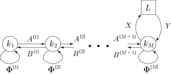
Figure 2. The $A_{M}$ linear quiver that corresponds to Figure 1 with the ranks of the flavour groups $L_{i}=0$, $i=1,\ldots,M-1$, $L_{M}=L$, and the ranks of the gauge groups $k_{1}\leq k_{2}\leq\ldots\leq k_{M}\leq L$.

We review the construction of orbifold-type codimension-2 defects in the $A_{1}$ quiver gauge theory that corresponds to the $\mathfrak{su}(2)$ spin-chain [1, 2, 3], then extend that to the $A_{M}$ quiver gauge theory that corresponds to the $\mathfrak{su}(M+1)$ spin-chain, described by the $A_{M}$ quiver in Figure 2.

4.1. Orbifold defect for $A_{1}$ quiver

Field	$U(k)$	twisted mass	$U(1)_{R}$
$X_{i}$	$\mathbf{k}$	$-m_{i}-\frac{\gamma}{2}$	$0$
$Y_{i}$	$\overline{\mathbf{k}}$	$m_{i}-\frac{\gamma}{2}$	$0$
$\Phi$	adj	$\gamma$	$2$

Table 3. The matter content of the $A_{1}$ quiver gauge theory that corresponds to the $\mathfrak{su}(2)$ spin-chain. Here $i=1,\ldots,L$, $k\leq L$.

Consider the A-twisted $U(k)$ GLSM on $S_{\hbar}^{\,2}$, with matter content as in Table 3, and the superpotential $W=\sum_{i=1}^{L}\sum_{a,b=1}^{k}X_{i,a}\Phi_{a,b}Y_{b,i}$, $k\leq L$. In this case, the equivariant characters (3.1) are given by

(4.1) $$\begin{split}&\chi_{\hbar}^{V}(\boldsymbol{u}_{k})=-\sum_{a\neq b}^{k}\frac{\mathrm{e}^{u_{a,b}}}{1-\mathrm{e}^{\hbar}},\qquad\chi_{\hbar}^{\Phi}(\boldsymbol{u}_{k})=\sum_{a,b=1}^{k}\frac{\mathrm{e}^{u_{a,b}+\gamma+\hbar}}{1-\mathrm{e}^{\hbar}},\\ &\chi_{\hbar}^{X_{i}}(\boldsymbol{u}_{k})=\sum_{a=1}^{k}\frac{\mathrm{e}^{u_{a}-m_{i}-\frac{\gamma}{2}}}{1-\mathrm{e}^{\hbar}},\qquad\chi_{\hbar}^{Y_{i}}(\boldsymbol{u}_{k})=\sum_{a=1}^{k}\frac{\mathrm{e}^{-u_{a}+m_{i}-\frac{\gamma}{2}}}{1-\mathrm{e}^{\hbar}}\end{split}$$

Now, we recall the construction of orbifold defects for the $A_{1}$ quiver in [1, 2, 3]. The orbifold defects inserted at the north (or south) pole of $S_{\hbar}^{\,2}$ are characterized by a discrete holonomy $\omega^{\,n}$, $n=0,1,\ldots,L-1$, with $\omega^{\,L}=1$, associated with a ${\mathbb{Z}}_{L}$ orbifold around the north (or south) pole, such that the gauge symmetry $U(k)$ and the flavor symmetry $U(L)$ are broken to a maximal torus. Firstly, for constructing such orbifold defects, we change the parameters

(4.2) $$m_{i}\ \to\ m_{i}+\left\lgroup i-1\right\rgroup\frac{\hbar}{L},\qquad u_{a}|_{\pm}\ \to\ u_{a}|_{\pm}+\left\lgroup I_{a}-1\right\rgroup\frac{\hbar}{L},\qquad\hbar\ \to\ \frac{\hbar}{L},$$

in the total equivariant character $\chi_{+\hbar}^{\mathrm{total}}(\boldsymbol{u}_{k}|_{+})$ or $\chi_{-\hbar}^{\mathrm{total}}(\boldsymbol{u}_{k}|_{-})$ in (2.5), which is composed of the expressions in (4.1), where

(4.3) $$\boldsymbol{I}_{k}=\{I_{1},\ldots,I_{k}\}\subset\boldsymbol{I}_{L}=\{1,\ldots,L\},\qquad I_{a}<I_{a+1},$$

is an ordered set that characterizes the orbifold defect. Next, taking the ${\mathbb{Z}}_{L}$ invariant part under $\hbar\to\hbar+2\pi\mathrm{i}n$, $n=0,1,\ldots,L-1$, of $\chi_{+\hbar}^{\mathrm{total}}(\boldsymbol{u}_{k}|_{+})$ or $\chi_{-\hbar}^{\mathrm{total}}(\boldsymbol{u}_{k}|_{-})$, we obtain

(4.4) $$\begin{split}&\chi_{\pm\hbar}^{\mathrm{total}}(\boldsymbol{u}_{k}|_{\pm})\\ &-\sum_{a=1}^{k}\left\lgroup\sum_{i=1}^{I_{a}-1}\mathrm{e}^{\pm u_{a}|_{\pm}\mp m_{i}-\frac{\gamma}{2}}+\sum_{i=I_{a}+1}^{L}\mathrm{e}^{\mp u_{a}|_{\pm}\pm m_{i}-\frac{\gamma}{2}}-\sum_{a<b}^{k}\left\lgroup\mathrm{e}^{\mp u_{a,b}|_{\pm}}+\mathrm{e}^{\pm u_{a,b}|_{\pm}+\gamma}\right\rgroup\right\rgroup,\end{split}$$

which follows from the following lemma.

Lemma 4.1 ([3]).

For any parameters $x$ and $\hbar$, and integers $I$ and $L$, performing the shift of parameters

(4.5) $$x\ \to\ x+I\,\frac{\hbar}{L},\qquad\hbar\ \to\ \frac{\hbar}{L},\qquad-L+1\leq I\leq L-1,$$

in $\mathrm{e}^{\pm x}/(1-\mathrm{e}^{\pm\hbar})$, leads to the ${\mathbb{Z}}_{L}$ invariant part

(4.6) $$\frac{\mathrm{e}^{\pm x}}{1-\mathrm{e}^{\pm\hbar}}\ \ \longrightarrow\ \ \begin{cases}\frac{\mathrm{e}^{\pm x}}{1-\mathrm{e}^{\pm\hbar}}\ \ &\textrm{if}\ \ -L+1\leq I\leq 0,\\ \frac{\mathrm{e}^{\pm x}}{1-\mathrm{e}^{\pm\hbar}}-\mathrm{e}^{\pm x}\ \ &\textrm{if}\ \ 1\leq I\leq L-1\end{cases}$$

Proof.

By

$$\frac{1}{1-\mathrm{e}^{\,\frac{\hbar}{L}}}=\frac{1+\mathrm{e}^{\,\frac{\hbar}{L}}+\mathrm{e}^{\,2\,\frac{\hbar}{L}}+\cdots+\mathrm{e}^{\,(L-1)\,\frac{\hbar}{L}}}{1-\mathrm{e}^{\,\hbar}},$$

the lemma is proved. ∎

Symmetrizing in the variables $\boldsymbol{u}_{k}$, the contribution of a defect inserted at the north (resp. south) pole of $S_{\hbar}^{\,2}$ to the integrand of the JK contour integral is $\psi_{\boldsymbol{I}_{k}}^{(L)}(\boldsymbol{u}_{k}|_{+};\boldsymbol{m}_{L})$ (resp. $\psi_{\boldsymbol{I}_{k}^{\vee}}^{(L)}(\boldsymbol{u}_{k}|_{-};\boldsymbol{m}_{L}^{\vee})$ with $I_{a}^{\vee}=L-I_{a}+1$ and $m_{i}^{\vee}=m_{L-i+1}$), where

(4.7) $$\psi_{\boldsymbol{I}_{k}}^{(L)}(\boldsymbol{u}_{k};\boldsymbol{m}_{L})=\mathop{\operatorname{Sym}}_{\boldsymbol{u}_{k}}\frac{\prod_{a=1}^{k}\left\lgroup\prod_{i=1}^{I_{a}-1}\left\lgroup u_{a}-m_{i}-\frac{\gamma}{2}\right\rgroup\cdot\prod_{i=I_{a}+1}^{L}\left\lgroup-u_{a}+m_{i}-\frac{\gamma}{2}\right\rgroup\right\rgroup}{\prod_{a<b}^{k}u_{b,a}\left\lgroup u_{a,b}+\gamma\right\rgroup}$$

Here $\mathop{\operatorname{Sym}}_{\,\boldsymbol{u}_{k}}$ stands for the symmetrization of a function $f(\boldsymbol{u}_{k})$ in the variables $\boldsymbol{u}_{k}$,

$$\mathop{\operatorname{Sym}}_{\boldsymbol{u}_{k}}\,f(\boldsymbol{u}_{k})=\sum_{\sigma\in\mathfrak{S}_{k}}f(u_{\sigma(1)},\ldots,u_{\sigma(k)}),$$

and $\mathfrak{S}_{k}$ is the symmetric group of degree $k$.

Proposition 4.2 ([1, 2, 3]).

Consider a normalization of the $A_{1}$ quiver orbifold defect as

(4.8) $$\widehat{\psi}_{\boldsymbol{I}_{k}}^{(L)}(\boldsymbol{u}_{k};\boldsymbol{m}_{L}) =(-1)^{kL+\sum_{a=1}^{k}I_{a}}\,\prod_{a<b}^{k}\left\lgroup\gamma^{\,2}-u_{a,b}^{\,2}\right\rgroup\times\psi_{\boldsymbol{I}_{k}}^{(L)}(\boldsymbol{u}_{k};\boldsymbol{m}_{L})$$

$$=\mathop{\operatorname{Sym}}_{\boldsymbol{u}_{k}}\,\omega_{\boldsymbol{I}_{k}}^{(L)}(\boldsymbol{u}_{k};\boldsymbol{m}_{L}),$$

where

(4.9) $$\omega_{\boldsymbol{I}_{k}}^{(L)}(\boldsymbol{u}_{k};\boldsymbol{m}_{L})=\prod_{a=1}^{k}\left\lgroup\prod_{i=1}^{I_{a}-1}\left\lgroup u_{a}-m_{i}-\frac{\gamma}{2}\right\rgroup\times\prod_{i=I_{a}+1}^{L}\left\lgroup u_{a}-m_{i}+\frac{\gamma}{2}\right\rgroup\right\rgroup\times\prod_{a<b}^{k}\frac{u_{a,b}-\gamma}{u_{a,b}}$$

Then, the defect $\widehat{\psi}_{\boldsymbol{I}_{k}}^{(L)}(\boldsymbol{u}_{k};\boldsymbol{m}_{L})$ gives the coordinate Bethe wavefunction of $\mathfrak{su}(2)$ XXX spin-$\frac{1}{2}$ chain.

Note that the defects inserted at the north pole and the south pole of $S_{\hbar}^{\,2}$ are given by

$$\widehat{\psi}_{\boldsymbol{I}_{k}}^{(L)}\left\lgroup\boldsymbol{u}_{k}|_{+};\boldsymbol{m}_{L}\right\rgroup\ \ \textrm{and}\ \ \widehat{\psi}_{\boldsymbol{I}_{k}^{\vee}}^{(L)}\left\lgroup\boldsymbol{u}_{k}|_{-};\boldsymbol{m}_{L}^{\vee}\right\rgroup,$$

respectively, where $I_{a}^{\vee}=L-I_{a}+1$ and $m_{i}^{\vee}=m_{L-i+1}$.

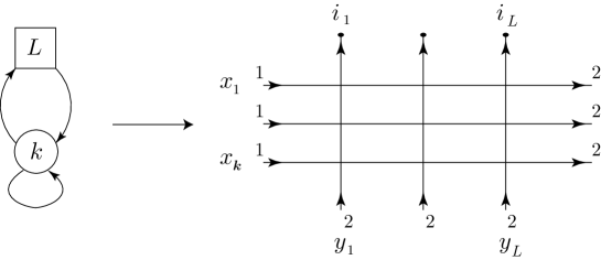
Figure 3. The $\mathfrak{su}(2)$ lattice configuration which describes the orbifold defect (4.8) for the $A_{1}$ quiver. Here $k\leq L$, and the indices $i_{\ell}\in\{1,2\}$, $\ell=1,\ldots,L$, represent spin-states, or equivalently, colours.

Remark 4.3.

Proposition 4.2 implies that, setting $u_{a}=x_{a}+1/2$, $m_{i}=y_{i}$, and $\gamma=1$, the defect $\widehat{\psi}_{\boldsymbol{I}_{k}}^{(L)}(\boldsymbol{u}_{k};\boldsymbol{m}_{L})$ in (4.8) agrees with the partition function (B.7) for the lattice configuration in Figure 3 of the rational $\mathfrak{su}(2)$ six-vertex model, where the set $\boldsymbol{I}_{L}$ labels the positions $\ell$ of colours $i_{\ell}\in\{1,2\}$, and the set $\boldsymbol{I}_{k}$ labels the positions $k$ of colour $1$.

Remark 4.4.

We have derived $\widehat{\psi}_{\boldsymbol{I}_{k}}^{(L)}(\boldsymbol{u}_{k};\boldsymbol{m}_{L})$ from the character in (4.4), using (2.7). Using (2.8) instead of (2.7), we obtain the coordinate Bethe wavefunction of the $\mathfrak{su}(2)$ XXZ spin-$\frac{1}{2}$ chain, and (4.9) is replaced by

(4.10) $$\omega_{\boldsymbol{I}_{k}}^{\mathrm{K},(L)}(\boldsymbol{u}_{k};\boldsymbol{m}_{L})=\prod_{a=1}^{k}\left\lgroup\prod_{i=1}^{I_{a}-1}\left[u_{a}-m_{i}-\frac{\gamma}{2}\right]\times\prod_{i=I_{a}+1}^{L}\left[u_{a}-m_{i}+\frac{\gamma}{2}\right]\right\rgroup\times\prod_{a<b}^{k}\frac{\left[u_{a,b}-\gamma\right]}{\left[u_{a,b}\right]},$$

where $[x]=2\sinh(x/2)$.

From the orbifold defect $\widehat{\psi}_{\boldsymbol{I}_{k}}^{(L)}(\boldsymbol{u}_{k};\boldsymbol{m}_{L})$, one obtains the $\mathfrak{su}(2)$ six-vertex model partial domain wall partition function (DWPF) [17]. In Appendix A, we prove the following proposition as a corollary of Propositions 4.2 and A.4.

Proposition 4.5 ($A_{1}$ partial DWPF).

Summing over the ordered set $\boldsymbol{I}_{k}$ in the orbifold defect $\widehat{\psi}_{\boldsymbol{I}_{k}}^{(L)}(\boldsymbol{u}_{k};\boldsymbol{m}_{L})$, we define a partition function

(4.11) $$\widehat{\mathcal{Z}}_{k}(\boldsymbol{u}_{k};\boldsymbol{m}_{L})=\sum_{\boldsymbol{I}_{k}\subset\{1,\ldots,L\}}\widehat{\psi}_{\boldsymbol{I}_{k}}^{(L)}(\boldsymbol{u}_{k};\boldsymbol{m}_{L})$$

Then, the partition function $\widehat{\mathcal{Z}}_{k}(\boldsymbol{u}_{k};\boldsymbol{m}_{L})$ agrees with the $\mathfrak{su}(2)$ six-vertex model partial DWPF, which has the determinant expression [17],

(4.12) $$\begin{split}\widehat{\mathcal{Z}}_{k}(\boldsymbol{u}_{k};\boldsymbol{m}_{L})&=\frac{\prod_{a=1}^{k}\prod_{i=1}^{L}\left\lgroup u_{a}-m_{i}-\frac{\gamma}{2}\right\rgroup\left\lgroup u_{a}-m_{i}+\frac{\gamma}{2}\right\rgroup}{\prod_{a<b}^{k}(u_{b}-u_{a})\cdot\prod_{i<j}^{L}(m_{i}-m_{j})}\\ &\qquad\times\left|\begin{array}[]{ccc}\frac{1}{\left\lgroup u_{1}-m_{1}-\frac{\gamma}{2}\right\rgroup\left\lgroup u_{1}-m_{1}+\frac{\gamma}{2}\right\rgroup}&\cdots&\frac{1}{\left\lgroup u_{1}-m_{L}-\frac{\gamma}{2}\right\rgroup\left\lgroup u_{1}-m_{L}+\frac{\gamma}{2}\right\rgroup}\\ \vdots&{}\hfil&\vdots\\ \frac{1}{\left\lgroup u_{k}-m_{1}-\frac{\gamma}{2}\right\rgroup\left\lgroup u_{k}-m_{1}+\frac{\gamma}{2}\right\rgroup}&\cdots&\frac{1}{\left\lgroup u_{k}-m_{L}-\frac{\gamma}{2}\right\rgroup\left\lgroup u_{k}-m_{L}+\frac{\gamma}{2}\right\rgroup}\\ m_{1}^{L-k-1}&\cdots&m_{L}^{L-k-1}\\ \vdots&{}\hfil&\vdots\\ m_{1}^{0}&\cdots&m_{L}^{0}\end{array}\right|,\end{split}$$

or equally [18, 19],

(4.13) $$\begin{split}\widehat{\mathcal{Z}}_{k}(\boldsymbol{u}_{k};\boldsymbol{m}_{L})&=\frac{\prod_{a=1}^{k}\prod_{i=1}^{L}\left\lgroup u_{a}-m_{i}+\frac{\gamma}{2}\right\rgroup}{\prod_{a<b}^{k}(u_{b}-u_{a})}\\ &\qquad\times\det\left\lgroup u_{a}^{b-1}\prod_{i=1}^{L}\frac{u_{a}-m_{i}-\frac{\gamma}{2}}{u_{a}-m_{i}+\frac{\gamma}{2}}-(u_{a}-\gamma)^{b-1}\right\rgroup_{a,b=1,\ldots,k}\end{split}$$

4.2. Orbifold defect for a simple $A_{M}$ quiver

We extend the above construction of the $A_{1}$ quiver orbifold defects to the simple $A_{M}$ linear quiver in Figure 2, with the matter content in Table 1. The equivariant characters are given in (3.1), with $L_{\,p}=0$, $p=1,\ldots,M-1$, and $k_{1}\leq k_{2}\leq\ldots\leq k_{M}\leq L$. To construct orbifold defects which break the gauge symmetry $U(k_{1})\times\cdots\times U(k_{M})$ and the flavor symmetry $U(L)$ to a maximal torus, as a generalization of the change of parameters (4.2), we consider

(4.14) $$m_{i}\ \to\ m_{i}+\left\lgroup i-1\right\rgroup\frac{\hbar}{L},\qquad u_{a}^{(p)}\big{|}_{\pm}\ \to\ u_{a}^{(p)}\big{|}_{\pm}+\left\lgroup I_{a}^{(p)}-1\right\rgroup\frac{\hbar}{L},\qquad\hbar\ \to\ \frac{\hbar}{L},$$

in the total equivariant character $\chi_{+\hbar}^{\mathrm{total}}(\boldsymbol{u}_{\boldsymbol{k}}^{M}|_{+})$ or $\chi_{-\hbar}^{\mathrm{total}}(\boldsymbol{u}_{\boldsymbol{k}}^{M}|_{-})$ in (2.5), where

(4.15) $$\boldsymbol{I}_{k_{1}}^{(1)}\subset\boldsymbol{I}_{k_{2}}^{(2)}\subset\cdots\subset\boldsymbol{I}_{k_{M}}^{(M)}\subset\boldsymbol{I}_{L}=\{1,\ldots,L\},\quad\boldsymbol{I}_{k_{\,p}}^{(p)}=\big{\{}I_{1}^{(p)},\ldots,I_{k_{\,p}}^{(p)}\big{\}},\quad I_{a}^{(p)}<I_{a+1}^{(p)},$$

Taking the ${\mathbb{Z}}_{L}$ invariant part of the total equivariant character under $\hbar\to\hbar+2\pi\mathrm{i}n$, $n=0,1,\ldots,L-1$, from Lemma 4.1 one finds

(4.16) $$\begin{split}&\chi_{\pm\hbar}^{\mathrm{total}}\left\lgroup\boldsymbol{u}_{\boldsymbol{k}}^{M}|_{\pm}\right\rgroup\\ &-\sum_{a=1}^{k_{M}}\left\lgroup\sum_{i=1}^{I_{a}^{(M)}-1}\mathrm{e}^{\pm u_{a}^{(M)}|_{\pm}\mp m_{i}-\frac{\gamma}{2}}+\sum_{i=I_{a}^{(M)}+1}^{L}\mathrm{e}^{\mp u_{a}^{(M)}|_{\pm}\pm m_{i}-\frac{\gamma}{2}}\right\rgroup\\ &+\sum_{p=1}^{M}\sum_{a<b}^{k_{\,p}}\left\lgroup\mathrm{e}^{\mp u_{a,b}^{(p)}|_{\pm}}+\mathrm{e}^{\pm u_{a,b}^{(p)}|_{\pm}+\gamma}\right\rgroup\\ &-\sum_{p=1}^{M-1}\sum_{a=1}^{k_{\,p}}\left\lgroup\sum_{b=1}^{\widetilde{I}_{a}^{(p)}-1}\mathrm{e}^{\pm u_{a}^{(p)}|_{\pm}\mp u_{b}^{(p+1)}|_{\pm}-\frac{\gamma}{2}}+\sum_{b=\widetilde{I}_{a}^{(p)}+1}^{k_{p+1}}\mathrm{e}^{\mp u_{a}^{(p)}|_{\pm}\pm u_{b}^{(p+1)}|_{\pm}-\frac{\gamma}{2}}\right\rgroup,\end{split}$$

where the set $\widetilde{\boldsymbol{I}}_{a}^{(p)}$ is defined by the map

(4.17) $$\boldsymbol{I}_{k_{\,p}}^{(p)}\subset\boldsymbol{I}_{k_{p+1}}^{(p+1)}\quad\to\quad\widetilde{\boldsymbol{I}}_{k_{\,p}}^{(p)}=\big{\{}\widetilde{I}_{1}^{(p)},\ldots,\widetilde{I}_{k_{\,p}}^{(p)}\big{\}}\subset\{1,\ldots,k_{p+1}\},$$

which can be explained as follows. $\boldsymbol{I}_{k_{\,p}}^{(p)}$ is a subset in the set $\boldsymbol{I}_{k_{p+1}}^{(p+1)}$, and $\widetilde{\boldsymbol{I}}_{k_{\,p}}^{(p)}$ is a subset in the set $\{1,\ldots,k_{p+1}\}$. Mapping the set $\boldsymbol{I}_{k_{p+1}}^{(p+1)}$ to the set $\{1,\ldots,k_{p+1}\}$ using the map $I_{a}^{(p+1)}\mapsto a$, $a=1,\ldots,p+1$, induces a map from the subset $\boldsymbol{I}_{k_{\,p}}^{(p)}$ to the subset $\widetilde{\boldsymbol{I}}_{k_{\,p}}^{(p)}$, which defines $\widetilde{\boldsymbol{I}}_{k_{\,p}}^{(p)}$. By (2.7), after symmetrization in the vector multiplet scalars $\boldsymbol{u}_{k_{1}},\ldots,\boldsymbol{u}_{k_{M}}$, one obtains the defect

(4.18) $$\psi_{\boldsymbol{I}_{\boldsymbol{k}}^{M}}^{(L)}\left\lgroup\boldsymbol{u}_{\boldsymbol{k}}^{M};\boldsymbol{m}_{L}\right\rgroup\\ =\mathop{\operatorname{Sym}}_{\boldsymbol{u}_{k_{1}}^{(1)},\ldots,\boldsymbol{u}_{k_{M}}^{(M)}}\prod_{p=1}^{M-1}\frac{\prod_{a=1}^{k_{\,p}}\left\lgroup\prod_{b=1}^{\widetilde{I}_{a}^{(p)}-1}\left\lgroup u_{a}^{(p)}-u_{b}^{(p+1)}-\frac{\gamma}{2}\right\rgroup\cdot\prod_{b=\widetilde{I}_{a}^{(p)}+1}^{k_{p+1}}\left\lgroup-u_{a}^{(p)}+u_{b}^{(p+1)}-\frac{\gamma}{2}\right\rgroup\right\rgroup}{\prod_{a<b}^{k_{\,p}}u_{b,a}^{(p)}\left\lgroup u_{a,b}^{(p)}+\gamma\right\rgroup}\\ \times\frac{\prod_{a=1}^{k_{M}}\left\lgroup\prod_{i=1}^{I_{a}^{(M)}-1}\left\lgroup u_{a}^{(M)}-m_{i}-\frac{\gamma}{2}\right\rgroup\cdot\prod_{i=I_{a}^{(M)}+1}^{L}\left\lgroup-u_{a}^{(M)}+m_{i}-\frac{\gamma}{2}\right\rgroup\right\rgroup}{\prod_{a<b}^{k_{M}}u_{b,a}^{(M)}\left\lgroup u_{a,b}^{(M)}+\gamma\right\rgroup},$$

which generalizes $\psi_{\boldsymbol{I}_{k}}^{(L)}(\boldsymbol{u}_{k};\boldsymbol{m}_{L})$ in (4.7), where $\boldsymbol{I}_{\boldsymbol{k}}^{M}=\{\boldsymbol{I}_{k_{1}}^{(1)},\ldots,\boldsymbol{I}_{k_{M}}^{(M)}\}$, and

$$\mathop{\operatorname{Sym}}_{\boldsymbol{u}_{k_{1}}^{(1)},\ldots,\boldsymbol{u}_{k_{M}}^{(M)}}=\mathop{\operatorname{Sym}}_{\boldsymbol{u}_{k_{1}}^{(1)}}\cdots\mathop{\operatorname{Sym}}_{\boldsymbol{u}_{k_{M}}^{(M)}}$$

Using a normalization similar to that in (4.8), we find the following proposition.

Proposition 4.6.

The orbifold defect, for the simple $A_{M}$ quiver in Figure 2,

(4.19) $$\widehat{\psi}_{\boldsymbol{I}_{\boldsymbol{k}}^{M}}^{(L)}\left\lgroup\boldsymbol{u}_{\boldsymbol{k}}^{M};\boldsymbol{m}_{L}\right\rgroup=\mathop{\operatorname{Sym}}_{\boldsymbol{u}_{k_{1}}^{(1)},\ldots,\boldsymbol{u}_{k_{M}}^{(M)}}\prod_{p=1}^{M-1}\omega_{\widetilde{\boldsymbol{I}}_{k_{\,p}}^{(p)}}^{(k_{p+1})}\left\lgroup\boldsymbol{u}_{k_{\,p}}^{(p)};\boldsymbol{u}_{k_{p+1}}^{(p+1)}\right\rgroup\times\omega_{\boldsymbol{I}_{k_{M}}^{(M)}}^{(L)}\left\lgroup\boldsymbol{u}_{k_{M}}^{(M)};\boldsymbol{m}_{L}\right\rgroup,$$

gives the nested coordinate Bethe wavefunction (see e.g. [20]) in the $\mathfrak{su}(M+1)$ XXX spin-chain with spins in the fundamental representation, where $\omega_{\boldsymbol{I}_{k}}^{(L)}(\boldsymbol{u}_{k};\boldsymbol{m}_{L})$ is defined in (4.9).

Remark 4.7.

Proposition 4.6 implies that, by the change of variables (B.2), the orbifold defect (4.19) coincides with the partition function (B.7) of a lattice configuration, with $L_{i}=0$, $i=1,\ldots,M-1$, and $L_{M}=L$, of the rational $\mathfrak{su}(M+1)$ XXX vertex model, where the set $\boldsymbol{I}_{L}$ labels the positions $\ell$ of all colours $i_{\ell}\in\{1,\ldots,M+1\}$, the set $\boldsymbol{I}_{k_{1}}^{(1)}$ labels the positions of colour $1$, and the set $\boldsymbol{I}_{k_{\,p}}^{\,(p)}\backslash\boldsymbol{I}_{k_{p-1}}^{(p-1)}$, $p=2,\ldots,M$, labels the positions of colour $p$.

Remark 4.8.

In [21], the orbifold defect (4.19) was geometrically constructed as an element in a stable basis [22] in the cotangent bundle of a partial flag variety (see also [23, 24]).

Remark 4.9.

Similarly to Remark 4.4, replacing $\omega_{\boldsymbol{I}_{k}}^{(L)}(\boldsymbol{u}_{k};\boldsymbol{m}_{L})$ with $\omega_{\boldsymbol{I}_{k}}^{\mathrm{K},(L)}(\boldsymbol{u}_{k};\boldsymbol{m}_{L})$ in the orbifold defect (4.19), one obtains the trigonometric expression which coincides with coordinate Bethe wavefunction of the corresponding XXZ spin-chain.

Proposition 4.10.

Summing over the ordered sets $\boldsymbol{I}_{\boldsymbol{k}}^{M}$, with a fixed set $\boldsymbol{I}_{k_{M}}^{(M)}$, in the defect (4.19), we define a partition function

(4.20) $$\widehat{\mathcal{Z}}_{\boldsymbol{I}_{k_{M}}^{(M)}}\left\lgroup\boldsymbol{u}_{\boldsymbol{k}}^{M};\boldsymbol{m}_{L}\right\rgroup=\sum_{\boldsymbol{I}_{k_{1}}^{(1)}\subset\boldsymbol{I}_{k_{2}}^{(2)}\subset\ldots\subset\boldsymbol{I}_{k_{M}}^{(M)}}\widehat{\psi}_{\boldsymbol{I}_{\boldsymbol{k}}^{M}}^{(L)}\left\lgroup\boldsymbol{u}_{\boldsymbol{k}}^{M};\boldsymbol{m}_{L}\right\rgroup$$

Then, the partition function factorizes into the $A_{1}$ quiver orbifold defect in (4.8) and the $\mathfrak{su}(2)$ six-vertex model partial DWPF (4.11),

(4.21) $$\widehat{\mathcal{Z}}_{\boldsymbol{I}_{k_{M}}^{(M)}}\left\lgroup\boldsymbol{u}_{\boldsymbol{k}}^{M};\boldsymbol{m}_{L}\right\rgroup=\prod_{p=1}^{M-1}\widehat{\mathcal{Z}}_{k_{\,p}}\left\lgroup\boldsymbol{u}_{k_{\,p}}^{(p)};\boldsymbol{u}_{k_{p+1}}^{(p+1)}\right\rgroup\times\widehat{\psi}_{\boldsymbol{I}_{k_{M}}^{(M)}}^{(L)}\left\lgroup\boldsymbol{u}_{k_{M}}^{(M)};\boldsymbol{m}_{L}\right\rgroup$$

Further,

(4.22) $$\sum_{\boldsymbol{I}_{k_{M}}^{(M)}\subset\{1,\ldots,L\}}\widehat{\mathcal{Z}}_{\boldsymbol{I}_{k_{M}}^{(M)}}\left\lgroup\boldsymbol{u}_{\boldsymbol{k}}^{M};\boldsymbol{m}_{L}\right\rgroup=\prod_{p=1}^{M-1}\widehat{\mathcal{Z}}_{k_{\,p}}\left\lgroup\boldsymbol{u}_{k_{\,p}}^{(p)};\boldsymbol{u}_{k_{p+1}}^{(p+1)}\right\rgroup\times\widehat{\mathcal{Z}}_{k_{M}}\left\lgroup\boldsymbol{u}_{k_{M}}^{(M)};\boldsymbol{m}_{L}\right\rgroup$$

Proof.

From 3 in Proposition A.3 and (A.2), the partition function $\widehat{\mathcal{Z}}_{k_{1}}(\boldsymbol{u}_{k_{1}}^{(1)};\boldsymbol{u}_{k_{2}}^{(2)})$ is a symmetric polynomial of $\boldsymbol{u}_{k_{2}}^{(2)}$, and then,

(4.23) $$\mathop{\operatorname{Sym}}_{\boldsymbol{u}_{k_{2}}^{(2)}}\,\widehat{\mathcal{Z}}_{k_{1}}\left\lgroup\boldsymbol{u}_{k_{1}}^{(1)};\boldsymbol{u}_{k_{2}}^{(2)}\right\rgroup\,\omega_{\widetilde{\boldsymbol{I}}_{k_{2}}^{(2)}}^{(k_{3})}\left\lgroup\boldsymbol{u}_{k_{2}}^{(2)};\boldsymbol{u}_{k_{3}}^{(3)}\right\rgroup=\widehat{\mathcal{Z}}_{k_{1}}\left\lgroup\boldsymbol{u}_{k_{1}}^{(1)};\boldsymbol{u}_{k_{2}}^{(2)}\right\rgroup\,\widehat{\psi}_{\widetilde{\boldsymbol{I}}_{k_{2}}^{(2)}}^{(k_{3})}\left\lgroup\boldsymbol{u}_{k_{2}}^{(2)};\boldsymbol{u}_{k_{3}}^{(3)}\right\rgroup$$

Repeating this symmetrization, one finds the factorizations (4.21) and (4.22). ∎

Remark 4.11.

In [25], the factorization (4.22) was shown for the $\mathfrak{su}(M+1)$ vertex model (see Remark 4.7), and was traced to a property (called ‘colour-independence’) of partition functions that satisfy certain boundary conditions.

5. Generalizations by Higgsing

In Section 5.1, we recall the Higgsing procedure in the $A_{M}$ quiver in Figure 1 without orbifold defects, in terms of the equivariant characters (3.1). In Sections 5.2 and 5.3, by applying the Higgsing to the orbifold construction in Section 4, we generalize the simple $A_{M}$ quiver orbifold defect (4.19) to more general $A_{2}$ then to $A_{M}$ quiver orbifold defects. In Section 5.4, we study the dual of Higgsing on the Bethe side of the Bethe/Gauge correspondence.

5.1. Higgsing

IIA	0	1	2	3	4	5	6	7	8	9
NS5	$-$	$-$	$-$	$-$	$-$	$-$
D2	$-$	$-$					$-$
D4	$-$	$-$						$-$	$-$	$-$

IIB	0	1	2	3	4	5	6	7	8	9
NS5	$-$	$-$	$-$	$-$	$-$	$-$
D3	$-$	$-$	$-$				$-$
D5	$-$	$-$	$-$					$-$	$-$	$-$

Table 4. On the left is a type-IIA brane configuration, and on the right is the type-IIB brane configuration in [16] that corresponds to it by T-duality along the $x^{2}$-direction (see also Figure 4).

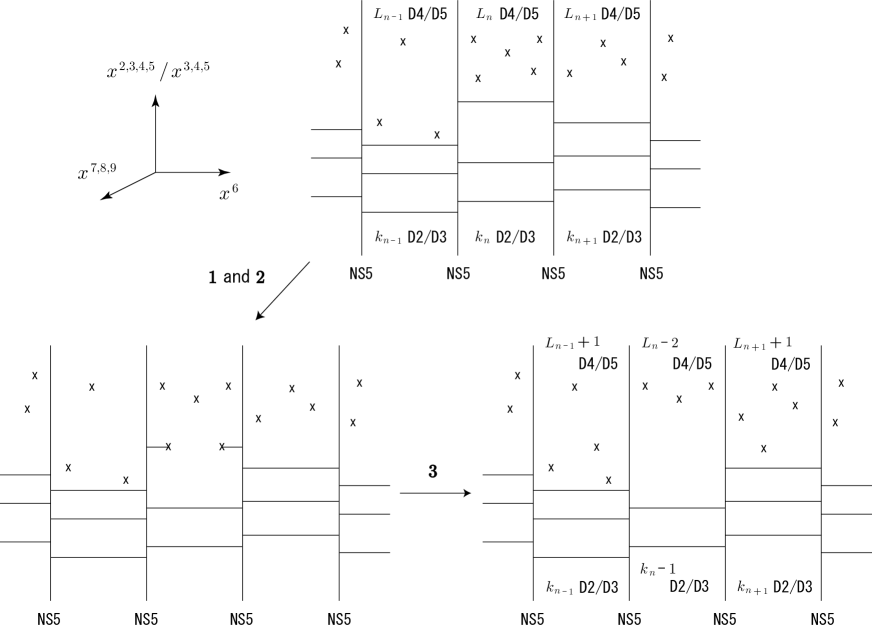
Figure 4. The Higgsing procedure including Hanany-Witten moves for type-IIA/IIB brane configuration [16], where the vertical (resp. horizontal) lines represent NS5 (resp. D2/D3) branes, and each x represents a D4/D5 brane. The corresponding quiver description is in Figure 5.

In [16], Gaiotto and Koroteev discussed a Higgsing procedure in terms of type-IIB brane realizations, in 3D $\mathcal{N}=2$ quiver gauge theories that are Bethe/Gauge dual to XXZ spin-chains. In Table 4 and Figure 4, we describe a type-IIA brane configuration, and a type-IIB brane configuration in [16] that corresponds to it by T-duality along the $x^{2}$-direction. By introducing the twisted mass $\gamma$ in Table 1, which breaks half the supersymmetry, these configurations describe, respectively, 2D $\mathcal{N}=(2,2)$ quiver gauge theories on the $(x^{0},x^{1})$-directions, and 3D $\mathcal{N}=2$ quiver gauge theories on the $(x^{0},x^{1},x^{2})$-directions. For the purposes of this work, the basic idea, as described in Figure 4, is

• to fine-tune the quiver data so that two D4/D5 branes are aligned at the same position in $(x^{2},x^{3},x^{4},x^{5})/(x^{3},x^{4},x^{5})$-directions, and a segment of a D2/D3 brane stretches between them,

• the D2/D3 segment that stretches between the two aligned D4/D5 branes is taken to infinity in the $(x^{7},x^{8},x^{9})$-directions, and finally,

• a sequence of Hanany-Witten moves of the two aligned D4/D5 branes, which are across NS5 branes, are used to simplify the resulting quiver .

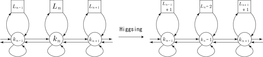
Figure 5. Higgsing the $n$-th gauge node of the $A_{M}$ linear quiver.

5.1.1. Higgsing the $A_{M}$ quiver on the left hand side of Figure 5

Following [16], the specialization of the parameters

(5.1) $$u_{k_{n}}^{(n)}=m_{L_{n}-1}^{(n)}-\frac{\gamma}{2}=m_{L_{n}}^{(n)}+\frac{\gamma}{2}=:\mu_{H},$$

Higgses the $n$-th gauge node of the $A_{M}$ quiver on the left hand side of Figure 5, and changes the quiver parameters as follows,

(5.2) $$\begin{split}&k_{\,p}\ \to\ k_{\,p},\ (\textrm{for}\ p\neq n),\qquad L_{\,p}\ \to\ L_{\,p},\ (\textrm{for}\ p\neq n,n\pm 1),\\ &k_{n}\ \to\ k_{n}-1,\qquad L_{n}\ \to\ L_{n}-2,\qquad L_{n\pm 1}\ \to\ L_{n\pm 1}+1,\end{split}$$

as depicted in the transition from the left hand side to the right hand side of Figure 5 [26].

5.1.2. Higgsing the equivariant characters (3.1)

Applying (5.1) to the characters, we obtain the Higgsed characters

(5.3) $$\chi_{H,\hbar}^{P}(\boldsymbol{u}):=\chi_{\hbar}^{P}(\boldsymbol{u})\big{|}_{\eqref{HW_move}},$$

where the following characters remain unchanged

(5.4) $$\begin{split}&\chi_{H,\hbar}^{V^{(p)}}\left\lgroup\boldsymbol{u}_{k_{\,p}}^{(p)}\right\rgroup=\chi_{\hbar}^{V^{(p)}}\left\lgroup\boldsymbol{u}_{k_{\,p}}^{(p)}\right\rgroup,\qquad\chi_{H,\hbar}^{\Phi^{(p)}}\left\lgroup\boldsymbol{u}_{k_{\,p}}^{(p)}\right\rgroup=\chi_{\hbar}^{\Phi^{(p)}}\left\lgroup\boldsymbol{u}_{k_{\,p}}^{(p)}\right\rgroup,\\ &\chi_{H,\hbar}^{X_{i}^{(p)}}\left\lgroup\boldsymbol{u}_{k_{\,p}}^{(p)}\right\rgroup=\chi_{\hbar}^{X_{i}^{(p)}}\left\lgroup\boldsymbol{u}_{k_{\,p}}^{(p)}\right\rgroup,\qquad\chi_{H,\hbar}^{Y_{i}^{(p)}}\left\lgroup\boldsymbol{u}_{k_{\,p}}^{(p)}\right\rgroup=\chi_{\hbar}^{Y_{i}^{(p)}}\left\lgroup\boldsymbol{u}_{k_{\,p}}^{(p)}\right\rgroup,\qquad\textrm{for}\ p\neq n,\\ &\chi_{H,\hbar}^{A^{(p^{\prime})}}\left\lgroup\boldsymbol{u}_{k_{p^{\prime}}}^{(p^{\prime})},\boldsymbol{u}_{k_{p^{\prime}+1}}^{(p^{\prime}+1)}\right\rgroup=\chi_{\hbar}^{A^{(p^{\prime})}}\left\lgroup\boldsymbol{u}_{k_{p^{\prime}}}^{(p^{\prime})},\boldsymbol{u}_{k_{p^{\prime}+1}}^{(p^{\prime}+1)}\right\rgroup,\\ &\chi_{H,\hbar}^{B^{(p^{\prime})}}\left\lgroup\boldsymbol{u}_{k_{p^{\prime}}}^{(p^{\prime})},\boldsymbol{u}_{k_{p^{\prime}+1}}^{(p^{\prime}+1)}\right\rgroup=\chi_{\hbar}^{B^{(p^{\prime})}}\left\lgroup\boldsymbol{u}_{k_{p^{\prime}}}^{(p^{\prime})},\boldsymbol{u}_{k_{p^{\prime}+1}}^{(p^{\prime}+1)}\right\rgroup,\qquad\textrm{for}\ p^{\prime}\neq n-1,n,\end{split}$$

while the following characters change

(5.5) $$\begin{split}&\chi_{H,\hbar}^{V^{(n)}}\left\lgroup\boldsymbol{u}_{k_{n}}^{(n)}\right\rgroup=\chi_{\hbar}^{V^{(n)}}\left\lgroup\boldsymbol{u}_{k_{n}-1}^{(n)}\right\rgroup-\sum_{a=1}^{k_{n}-1}\frac{\mathrm{e}^{u_{a}^{(n)}-\mu_{H}}+\mathrm{e}^{-u_{a}^{(n)}+\mu_{H}}}{1-\mathrm{e}^{\hbar}},\\ &\chi_{H,\hbar}^{\Phi^{(n)}}\left\lgroup\boldsymbol{u}_{k_{n}}^{(n)}\right\rgroup=\chi_{\hbar}^{\Phi^{(n)}}\left\lgroup\boldsymbol{u}_{k_{n}-1}^{(n)}\right\rgroup+\sum_{a=1}^{k_{n}-1}\frac{\mathrm{e}^{u_{a}^{(n)}-\mu_{H}+\gamma+\hbar}+\mathrm{e}^{-u_{a}^{(n)}+\mu_{H}+\gamma+\hbar}}{1-\mathrm{e}^{\hbar}}+\frac{\mathrm{e}^{\gamma+\hbar}}{1-\mathrm{e}^{\hbar}},\\ &\sum_{i=1}^{L_{n}}\chi_{H,\hbar}^{X_{i}^{(n)}}\left\lgroup\boldsymbol{u}_{k_{n}}^{(n)}\right\rgroup=\sum_{i=1}^{L_{n}-2}\chi_{\hbar}^{X_{i}^{(n)}}\left\lgroup\boldsymbol{u}_{k_{n}-1}^{(n)}\right\rgroup+\sum_{a=1}^{k_{n}-1}\frac{\mathrm{e}^{u_{a}^{(n)}-\mu_{H}-\gamma}+\mathrm{e}^{u_{a}^{(n)}-\mu_{H}}}{1-\mathrm{e}^{\hbar}}+\sum_{i=1}^{L_{n}}\frac{\mathrm{e}^{\mu_{H}-m_{i}^{(n)}-\frac{\gamma}{2}}}{1-\mathrm{e}^{\hbar}},\\ &\sum_{i=1}^{L_{n}}\chi_{H,\hbar}^{Y_{i}^{(n)}}\left\lgroup\boldsymbol{u}_{k_{n}}^{(n)}\right\rgroup=\sum_{i=1}^{L_{n}-2}\chi_{\hbar}^{Y_{i}^{(n)}}\left\lgroup\boldsymbol{u}_{k_{n}-1}^{(n)}\right\rgroup+\sum_{a=1}^{k_{n}-1}\frac{\mathrm{e}^{-u_{a}^{(n)}+\mu_{H}}+\mathrm{e}^{-u_{a}^{(n)}+\mu_{H}-\gamma}}{1-\mathrm{e}^{\hbar}}+\sum_{i=1}^{L_{n}}\frac{\mathrm{e}^{-\mu_{H}+m_{i}^{(n)}-\frac{\gamma}{2}}}{1-\mathrm{e}^{\hbar}},\end{split}$$

and

(5.6) $$\begin{split}&\chi_{H,\hbar}^{A^{(n-1)}}\left\lgroup\boldsymbol{u}_{k_{n-1}}^{(n-1)},\boldsymbol{u}_{k_{n}}^{(n)}\right\rgroup=\chi_{\hbar}^{A^{(n-1)}}\left\lgroup\boldsymbol{u}_{k_{n-1}}^{(n-1)},\boldsymbol{u}_{k_{n}-1}^{(n)}\right\rgroup+\sum_{a=1}^{k_{n-1}}\frac{\mathrm{e}^{u_{a}^{(n-1)}-\mu_{H}-\frac{\gamma}{2}}}{1-\mathrm{e}^{\hbar}},\\ &\chi_{H,\hbar}^{A^{(n)}}\left\lgroup\boldsymbol{u}_{k_{n}}^{(n)},\boldsymbol{u}_{k_{n+1}}^{(n+1)}\right\rgroup=\chi_{\hbar}^{A^{(n)}}\left\lgroup\boldsymbol{u}_{k_{n}-1}^{(n)},\boldsymbol{u}_{k_{n+1}}^{(n+1)}\right\rgroup+\sum_{a=1}^{k_{n+1}}\frac{\mathrm{e}^{\mu_{H}-u_{a}^{(n+1)}-\frac{\gamma}{2}}}{1-\mathrm{e}^{\hbar}},\\ &\chi_{H,\hbar}^{B^{(n-1)}}\left\lgroup\boldsymbol{u}_{k_{n-1}}^{(n-1)},\boldsymbol{u}_{k_{n}}^{(n)}\right\rgroup=\chi_{\hbar}^{B^{(n-1)}}\left\lgroup\boldsymbol{u}_{k_{n-1}}^{(n-1)},\boldsymbol{u}_{k_{n}-1}^{(n)}\right\rgroup+\sum_{a=1}^{k_{n-1}}\frac{\mathrm{e}^{-u_{a}^{(n-1)}+\mu_{H}-\frac{\gamma}{2}}}{1-\mathrm{e}^{\hbar}},\\ &\chi_{H,\hbar}^{B^{(n)}}\left\lgroup\boldsymbol{u}_{k_{n}}^{(n)},\boldsymbol{u}_{k_{n+1}}^{(n+1)}\right\rgroup=\chi_{\hbar}^{B^{(n)}}\left\lgroup\boldsymbol{u}_{k_{n}-1}^{(n)},\boldsymbol{u}_{k_{n+1}}^{(n+1)}\right\rgroup+\sum_{a=1}^{k_{n+1}}\frac{\mathrm{e}^{-\mu_{H}+u_{a}^{(n+1)}-\frac{\gamma}{2}}}{1-\mathrm{e}^{\hbar}}\end{split}$$

The sum of the Higgsed characters in (LABEL:hg_ch_AM_2) becomes

(5.7) $$\chi_{H,\hbar}^{V^{(n)}}\left\lgroup\boldsymbol{u}_{k_{n}}^{(n)}\right\rgroup+\chi_{H,\hbar}^{\Phi^{(n)}}\left\lgroup\boldsymbol{u}_{k_{n}}^{(n)}\right\rgroup+\sum_{i=1}^{L_{n}}\left\lgroup\chi_{H,\hbar}^{X_{i}^{(n)}}\left\lgroup\boldsymbol{u}_{k_{n}}^{(n)}\right\rgroup+\chi_{H,\hbar}^{Y_{i}^{(n)}}\left\lgroup\boldsymbol{u}_{k_{n}}^{(n)}\right\rgroup\right\rgroup\\ =\chi_{\hbar}^{V^{(n)}}\left\lgroup\boldsymbol{u}_{k_{n}-1}^{(n)}\right\rgroup+\chi_{\hbar}^{\Phi^{(n)}}\left\lgroup\boldsymbol{u}_{k_{n}-1}^{(n)}\right\rgroup+\sum_{i=1}^{L_{n}-2}\left\lgroup\chi_{\hbar}^{X_{i}^{(n)}}\left\lgroup\boldsymbol{u}_{k_{n}-1}^{(n)}\right\rgroup+\chi_{\hbar}^{Y_{i}^{(n)}}\left\lgroup\boldsymbol{u}_{k_{n}-1}^{(n)}\right\rgroup\right\rgroup\\ \quad+\sum_{a=1}^{k_{n}-1}\left\lgroup\frac{\mathrm{e}^{-u_{a}^{(n)}+\mu_{H}-\gamma}}{1-\mathrm{e}^{\hbar}}-\frac{\mathrm{e}^{u_{a}^{(n)}-\mu_{H}+\gamma}}{1-\mathrm{e}^{-\hbar}}\right\rgroup+\sum_{a=1}^{k_{n}-1}\left\lgroup\frac{\mathrm{e}^{u_{a}^{(n)}-\mu_{H}-\gamma}}{1-\mathrm{e}^{\hbar}}-\frac{\mathrm{e}^{-u_{a}^{(n)}+\mu_{H}+\gamma}}{1-\mathrm{e}^{-\hbar}}\right\rgroup\\ +\frac{\mathrm{e}^{\gamma+\hbar}}{1-\mathrm{e}^{\hbar}}+\sum_{i=1}^{L_{n}}\frac{\mathrm{e}^{\mu_{H}-m_{i}^{(n)}-\frac{\gamma}{2}}}{1-\mathrm{e}^{\hbar}}+\sum_{i=1}^{L_{n}}\frac{\mathrm{e}^{-\mu_{H}+m_{i}^{(n)}-\frac{\gamma}{2}}}{1-\mathrm{e}^{\hbar}}$$

By considering the partition function (2.7) or (2.8), one finds that the contributions from the second line on the right hand side yield sign factors, while the third line does not depend on the variables $u_{a}^{(p)}$ and can be decoupled from the quiver gauge theory. One also finds that the extra factors of the first and third (resp. second and fourth) characters in (LABEL:hg_ch_AM_3),

(5.8) $$\sum_{a=1}^{k_{n-1}}\frac{\mathrm{e}^{u_{a}^{(n-1)}-\mu_{H}-\frac{\gamma}{2}}}{1-\mathrm{e}^{\hbar}}+\sum_{a=1}^{k_{n-1}}\frac{\mathrm{e}^{-u_{a}^{(n-1)}+\mu_{H}-\frac{\gamma}{2}}}{1-\mathrm{e}^{\hbar}},\quad\textrm{resp.}\ \sum_{a=1}^{k_{n+1}}\frac{\mathrm{e}^{u_{a}^{(n+1)}-\mu_{H}-\frac{\gamma}{2}}}{1-\mathrm{e}^{\hbar}}+\sum_{a=1}^{k_{n+1}}\frac{\mathrm{e}^{-u_{a}^{(n+1)}+\mu_{H}-\frac{\gamma}{2}}}{1-\mathrm{e}^{\hbar}},$$

agree with the contributions from extra (anti-)fundamental matter with mass parameter $\mu_{H}$ at the $(n-1)$-th (resp. $(n+1)$-th) gauge node. As a result, the transition (5.2), under the specialization (5.1), is confirmed.

5.2. Orbifold defect for $A_{2}$ quiver

In this subsection, we apply the Higgsing to the orbifold construction in Section 4 and generalize the simple $A_{M}$ quiver orbifold defects for $M=2$ constructed in Section 4.2. The case of general $M$ will be discussed in Section 5.3.

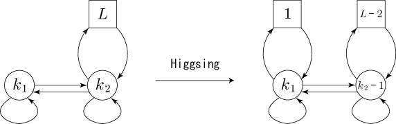
Figure 6. Higgsing the $A_{2}$ linear quiver.

5.2.1. Higgsing the $A_{2}$ quiver gauge theory in Figure 6

We set the $A_{2}$ quiver data $k_{1}\leq k_{2}\leq L-1$, so that the specialization (5.1) becomes

(5.9) $$u_{k_{2}}^{(2)}=m_{L-1}-\frac{\gamma}{2}=m_{L}+\frac{\gamma}{2}=:\mu_{H}$$

As before, the twisted masses $m_{L-1}$ and $m_{L}$ decouple after Higgsing, and compared with the discussion in Section 4.2, one only needs to consider the second factors on the right hand side in the Higgsed characters (LABEL:hg_ch_AM_3).

5.2.2. Construction of $A_{2}$ quiver orbifold defects

Instead of the change of parameters (4.14), we consider

(5.10) $$\begin{split}&\mu_{H}\ \to\ \mu_{H}+\left\lgroup L-2\right\rgroup\frac{\hbar}{L-1},\\ &m_{i}\ \to\ m_{i}+\left\lgroup i-1\right\rgroup\frac{\hbar}{L-1},\qquad i=1,\ldots,L-2,\\ &u_{a}^{(1)}\big{|}_{\pm}\ \to\ u_{a}^{(1)}\big{|}_{\pm}+\left\lgroup I_{a}^{(1)}-1\right\rgroup\frac{\hbar}{L-1},\qquad a=1,\ldots,k_{1},\\ &u_{a}^{(2)}\big{|}_{\pm}\ \to\ u_{a}^{(2)}\big{|}_{\pm}+\left\lgroup I_{a}^{(2)}-1\right\rgroup\frac{\hbar}{L-1},\qquad a=1,\ldots,k_{2}-1,\qquad\hbar\ \to\ \frac{\hbar}{L-1},\end{split}$$

which is consistent with Higgsing, where

(5.11) $$\boldsymbol{I}_{k_{1}}^{(1)}\subset\boldsymbol{I}_{k_{2}-1}^{(2)}\uplus\{L-1\}\subset\{1,\ldots,L-1\},\quad I_{a}^{(p)}<I_{a+1}^{(p)},$$

and the symbol $\uplus$ denotes the pairwise disjoint union. Then, as a generalization of (4.19) for $M=2$, we obtain an orbifold defect

(5.12) $$\widehat{\psi}_{\boldsymbol{I}_{k_{1}}^{(1)},\boldsymbol{I}_{k_{2}-1}^{(2)}}^{(1|1,L-2)}\left\lgroup\boldsymbol{u}_{k_{1}}^{(1)},\boldsymbol{u}_{k_{2}-1}^{(2)};\mu_{H},\boldsymbol{m}_{L-2}\right\rgroup=\\ \mathop{\operatorname{Sym}}_{\boldsymbol{u}_{k_{1}}^{(1)},\boldsymbol{u}_{k_{2}-1}^{(2)}}\omega_{\widetilde{\boldsymbol{I}}_{k_{1}}^{(1)}}^{(k_{2})}\left\lgroup\boldsymbol{u}_{k_{1}}^{(1)};\boldsymbol{u}_{k_{2}-1}^{(2)},\mu_{H}\right\rgroup\,\omega_{\boldsymbol{I}_{k_{2}-1}^{(2)}}^{(L-2)}\left\lgroup\boldsymbol{u}_{k_{2}-1}^{(2)};\boldsymbol{m}_{L-2}\right\rgroup,$$

where $\omega_{\boldsymbol{I}_{k}}^{(L)}(\boldsymbol{u}_{k};\boldsymbol{m}_{L})$ is defined in (4.9), and $\widetilde{\boldsymbol{I}}_{k_{1}}^{(1)}$ is defined by the map (4.17) for $\boldsymbol{I}_{k_{1}}^{(1)}\subset\boldsymbol{I}_{k_{2}-1}^{(2)}\uplus\{L-1\}$. Note that, instead of the change of parameters (5.10), by considering

(5.13) $$\begin{split}&\mu_{H}\ \to\ \mu_{H},\\ &m_{i}\ \to\ m_{i}+i\,\frac{\hbar}{L-1},\qquad i=1,\ldots,L-2,\\ &u_{a}^{(1)}\big{|}_{\pm}\ \to\ u_{a}^{(1)}\big{|}_{\pm}+\left\lgroup I_{a}^{(1)}-1\right\rgroup\frac{\hbar}{L-1},\qquad a=1,\ldots,k_{1},\\ &u_{a}^{(2)}\big{|}_{\pm}\ \to\ u_{a}^{(2)}\big{|}_{\pm}+\left\lgroup I_{a}^{(2)}-1\right\rgroup\,\frac{\hbar}{L-1},\qquad a=1,\ldots,k_{2}-1,\qquad\hbar\ \to\ \frac{\hbar}{L-1},\end{split}$$

with

(5.14) $$\boldsymbol{I}_{k_{1}}^{(1)}\subset\{1\}\uplus\boldsymbol{I}_{k_{2}-1}^{(2)}\subset\{1,\ldots,L-1\},\quad I_{a}^{(p)}<I_{a+1}^{(p)},$$

we obtain an another orbifold defect

(5.15) $$\widehat{\psi}_{\boldsymbol{I}_{k_{1}}^{(1)},\boldsymbol{I}_{k_{2}-1}^{(2)}}^{(2|1,L-2)}\left\lgroup\boldsymbol{u}_{k_{1}}^{(1)},\boldsymbol{u}_{k_{2}-1}^{(2)};\mu_{H},\boldsymbol{m}_{L-2}\right\rgroup=\\ \mathop{\operatorname{Sym}}_{\boldsymbol{u}_{k_{1}}^{(1)},\boldsymbol{u}_{k_{2}-1}^{(2)}}\omega_{\widetilde{\boldsymbol{I}}_{k_{1}}^{(1)}}^{(k_{2})}\left\lgroup\boldsymbol{u}_{k_{1}}^{(1)};\mu_{H},\boldsymbol{u}_{k_{2}-1}^{(2)}\right\rgroup\,\omega_{\widetilde{\boldsymbol{I}}_{k_{2}-1}^{(2)}}^{(L-2)}\left\lgroup\boldsymbol{u}_{k_{2}-1}^{(2)};\boldsymbol{m}_{L-2}\right\rgroup,$$

where $\widetilde{I}_{a}^{(2)}=I_{a}^{(2)}-1$.

5.2.3. More general $A_{2}$ quiver orbifold defects

One can apply the above Higgsing procedure repeatedly. Consider the $A_{2}$ quiver in Figure 1 with $M=2$, set $k_{1}\leq L_{1}+k_{2}\leq L_{1}+L_{2}$, and apply the change of parameters

(5.16) $$\begin{split}&m_{i}^{(1)}\ \to\ m_{i}^{(1)}+\left\lgroup L_{2}+i-1\right\rgroup\frac{\hbar}{L_{1}+L_{2}},\\ &m_{i}^{(2)}\ \to\ m_{i}^{(2)}+\left\lgroup i-1\right\rgroup\frac{\hbar}{L_{1}+L_{2}},\\ &u_{a}^{(p)}\big{|}_{\pm}\ \to\ u_{a}^{(p)}\big{|}_{\pm}+\left\lgroup I_{a}^{(p)}-1\right\rgroup\frac{\hbar}{L_{1}+L_{2}},\qquad\hbar\ \to\ \frac{\hbar}{L_{1}+L_{2}},\end{split}$$

to the equivariant characters (3.1), with $M=2$, where

(5.17) $$\boldsymbol{I}_{k_{1}}^{(1)}\subset\boldsymbol{I}_{k_{2}}^{(2)}\uplus\{L_{2}+1,\ldots,L_{1}+L_{2}\}\subset\{1,\ldots,L_{1}+L_{2}\},\quad I_{a}^{(p)}<I_{a+1}^{(p)}.$$

As a result, we find an orbifold defect for the $A_{2}$ quiver,

(5.18) $$\widehat{\psi}_{\boldsymbol{I}_{k_{1}}^{(1)},\boldsymbol{I}_{k_{2}}^{(2)}}^{(1|L_{1},L_{2})}\left\lgroup\boldsymbol{u}_{k_{1}}^{(1)},\boldsymbol{u}_{k_{2}}^{(2)};\boldsymbol{m}_{L_{1}}^{(1)},\boldsymbol{m}_{L_{2}}^{(2)}\right\rgroup=\\ \mathop{\operatorname{Sym}}_{\boldsymbol{u}_{k_{1}}^{(1)},\boldsymbol{u}_{k_{2}}^{(2)}}\omega_{\widetilde{\boldsymbol{I}}_{k_{1}}^{(1)}}^{(L_{1}+k_{2})}\left\lgroup\boldsymbol{u}_{k_{1}}^{(1)};\boldsymbol{u}_{k_{2}}^{(2)},\boldsymbol{m}_{L_{1}}^{(1)}\right\rgroup\,\omega_{\boldsymbol{I}_{k_{2}}^{(2)}}^{(L_{2})}\left\lgroup\boldsymbol{u}_{k_{2}}^{(2)};\boldsymbol{m}_{L_{2}}^{(2)}\right\rgroup,$$

which generalizes the defect (5.12). Similarly, instead of (5.16), by considering

(5.19) $$\begin{split}&m_{i}^{(1)}\ \to\ m_{i}^{(1)}+\left\lgroup i-1\right\rgroup\frac{\hbar}{L_{1}+L_{2}},\\ &m_{i}^{(2)}\ \to\ m_{i}^{(2)}+\left\lgroup L_{1}+i-1\right\rgroup\frac{\hbar}{L_{1}+L_{2}},\\ &u_{a}^{(p)}\big{|}_{\pm}\ \to\ u_{a}^{(p)}\big{|}_{\pm}+\left\lgroup I_{a}^{(p)}-1\right\rgroup\frac{\hbar}{L_{1}+L_{2}},\qquad\hbar\ \to\ \frac{\hbar}{L_{1}+L_{2}},\end{split}$$

with

(5.20) $$\boldsymbol{I}_{k_{1}}^{(1)}\subset\{1,\ldots,L_{1}\}\uplus\boldsymbol{I}_{k_{2}}^{(2)}\subset\{1,\ldots,L_{1}+L_{2}\},\quad I_{a}^{(p)}<I_{a+1}^{(p)},$$

we find an another orbifold defect for the $A_{2}$ quiver,

(5.21) $$\widehat{\psi}_{\boldsymbol{I}_{k_{1}}^{(1)},\boldsymbol{I}_{k_{2}}^{(2)}}^{(2|L_{1},L_{2})}\left\lgroup\boldsymbol{u}_{k_{1}}^{(1)},\boldsymbol{u}_{k_{2}}^{(2)};\boldsymbol{m}_{L_{1}}^{(1)},\boldsymbol{m}_{L_{2}}^{(2)}\right\rgroup=\\ \mathop{\operatorname{Sym}}_{\boldsymbol{u}_{k_{1}}^{(1)},\boldsymbol{u}_{k_{2}}^{(2)}}\omega_{\widetilde{\boldsymbol{I}}_{k_{1}}^{(1)}}^{(L_{1}+k_{2})}\left\lgroup\boldsymbol{u}_{k_{1}}^{(1)};\boldsymbol{m}_{L_{1}}^{(1)},\boldsymbol{u}_{k_{2}}^{(2)}\right\rgroup\,\omega_{\widetilde{\boldsymbol{I}}_{k_{2}}^{(2)}}^{(L_{2})}\left\lgroup\boldsymbol{u}_{k_{2}}^{(2)};\boldsymbol{m}_{L_{2}}^{(2)}\right\rgroup,$$

which generalizes the defect (5.15), where $\widetilde{I}_{a}^{(2)}=I_{a}^{(2)}-L_{1}$.

5.3. Orbifold defect for $A_{M}$ quiver

It is straightforward to generalize the above constructions of the orbifold defects (5.18) and (5.21) to the $A_{M}$ quiver in Figure 1 (see Table 1 for the matter content), where we set

(5.22) $$k_{\,p}\leq L_{\,p}+k_{p+1},\quad k_{M}\leq L_{M},\quad p=1,\ldots,M-1$$

The orbifold defects for the $A_{2}$ quiver are composed of the orbifold defect $\omega_{\boldsymbol{I}_{k}}^{(L)}(\boldsymbol{u}_{k};\boldsymbol{m}_{L})$ in (4.9) for the $A_{1}$ quiver, and it is useful to define

(5.23) $$\begin{split}&\omega_{\boldsymbol{I}_{k}}^{(1|\ell+L)}(\boldsymbol{u}_{k};\boldsymbol{v}_{\ell},\boldsymbol{m}_{L}):=\omega_{\boldsymbol{I}_{k}}^{(\ell+L)}(\boldsymbol{u}_{k};\boldsymbol{v}_{\ell},\boldsymbol{m}_{L}),\\ &\omega_{\boldsymbol{I}_{k}}^{(2|\ell+L)}(\boldsymbol{u}_{k};\boldsymbol{v}_{\ell},\boldsymbol{m}_{L}):=\omega_{\boldsymbol{I}_{k}}^{(\ell+L)}(\boldsymbol{u}_{k};\boldsymbol{m}_{L},\boldsymbol{v}_{\ell})\end{split}$$

Now, from the equivariant characters (3.1), we find orbifold defects for the $A_{M}$ quiver, which generalize the simple $A_{M}$ quiver orbifold defect (4.19),

(5.24) $$\widehat{\psi}_{\boldsymbol{I}_{\boldsymbol{k}}^{M}}^{(\boldsymbol{S}|\boldsymbol{L})}\left\lgroup\boldsymbol{u}_{\boldsymbol{k}}^{M};\boldsymbol{m}_{\boldsymbol{L}}^{M}\right\rgroup=\\ \mathop{\operatorname{Sym}}_{\boldsymbol{u}_{k_{1}}^{(1)},\ldots,\boldsymbol{u}_{k_{M}}^{(M)}}\prod_{p=1}^{M-1}\omega_{\widetilde{\boldsymbol{I}}_{k_{\,p}}^{(p)}}^{(s_{p}|k_{p+1}+L_{\,p})}\left\lgroup\boldsymbol{u}_{k_{\,p}}^{(p)};\boldsymbol{u}_{k_{p+1}}^{(p+1)},\boldsymbol{m}_{L_{\,p}}^{(p)}\right\rgroup\times\omega_{\widetilde{\boldsymbol{I}}_{k_{M}}^{(M)}}^{(L_{M})}\left\lgroup\boldsymbol{u}_{k_{M}}^{(M)};\boldsymbol{m}_{L_{M}}^{(M)}\right\rgroup,$$

which is characterized by the set $\boldsymbol{S}=\{s_{1},\ldots,s_{M-1}\}$, $s_{p}\in\{1,2\}$, and the sets $\boldsymbol{I}_{\boldsymbol{k}}^{M}$, with the inclusion relations

(5.25) $$\begin{split}&\boldsymbol{I}_{k_{\,p}}^{(p)}\subset\widehat{\boldsymbol{I}}_{k_{p+1}+L_{\,p}}^{(p+1)}:=\begin{cases}\boldsymbol{I}_{k_{p+1}}^{(p+1)}\uplus\{L_{\,p}^{(\boldsymbol{S})}+L_{p+1}+1,\ldots,L_{\,p}^{(\boldsymbol{S})}+L_{\,p}+L_{p+1}\}\ \ &\textrm{if}\ s_{p}=1,\\ \{L_{\,p}^{(\boldsymbol{S})}+1,\ldots,L_{\,p}^{(\boldsymbol{S})}+L_{\,p}\}\uplus\boldsymbol{I}_{k_{p+1}}^{(p+1)}\ \ &\textrm{if}\ s_{p}=2,\end{cases}\\ &\hskip 16.00008pt\subset\{L_{\,p}^{(\boldsymbol{S})}+1,\ldots,L_{\,p}^{(\boldsymbol{S})}+L_{\,p}+L_{p+1}\},\qquad p=1,\ldots,M-1,\\ &\boldsymbol{I}_{k_{M}}^{(M)}\subset\widehat{\boldsymbol{I}}_{L_{M}}^{(M+1)}:=\{L_{M}^{(\boldsymbol{S})}+1,\ldots,L_{M}^{(\boldsymbol{S})}+L_{M}\}\end{split}$$

Here $L_{\,p}^{(\boldsymbol{S})}=\sum_{q=1}^{p-1}L_{q}\delta_{s_{q},2}$, and the sets $\widetilde{\boldsymbol{I}}_{\boldsymbol{k}}^{M}$ are defined by the map (4.17), for the above inclusion relations. We claim that, by the reparametrizations (B.2), the orbifold defect (5.24) coincides with the partition function (B.7) for a lattice configuration of the $\mathfrak{su}(M+1)$ vertex model,

(5.26) $$\widehat{\psi}_{\boldsymbol{I}_{\boldsymbol{k}}^{M}}^{(\boldsymbol{S}|\boldsymbol{L})}\left\lgroup\boldsymbol{u}_{\boldsymbol{k}}^{M};\boldsymbol{m}_{\boldsymbol{L}}^{M}\right\rgroup=\widehat{\psi}_{\mathrm{L},\boldsymbol{i}_{\boldsymbol{L}}^{M}}^{(\boldsymbol{S}|\boldsymbol{L})}\left\lgroup\boldsymbol{x}_{\boldsymbol{k}}^{M};\boldsymbol{y}_{\boldsymbol{L}}^{M}\right\rgroup,$$

where $\widehat{\boldsymbol{I}}_{k_{p+1}+L_{\,p}}^{(p+1)}\backslash\boldsymbol{I}_{k_{p+1}}^{(p+1)}$, $p=1,\ldots,M-1$, and $\widehat{\boldsymbol{I}}_{L_{M}}^{(M+1)}$ label the positions $\ell$ of colours $i_{\ell}^{(p)}\in\{1,\ldots,p+1\}$ and $i_{\ell}^{(M)}\in\{1,\ldots,M+1\}$, respectively, the set $\boldsymbol{I}_{k_{1}}^{(1)}$ labels the positions of colour $1$, the set $\widehat{\boldsymbol{I}}_{k_{\,p}+L_{p-1}}^{(p)}\backslash\boldsymbol{I}_{k_{p-1}}^{(p-1)}$, $p=2,\ldots,M$, labels the positions of colour $p$, and the set $\widehat{\boldsymbol{I}}_{L_{M}}^{(M+1)}\backslash\boldsymbol{I}_{k_{M}}^{(M)}$ labels the positions of colour $M+1$.

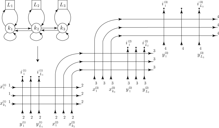
Figure 7. An $\mathfrak{su}(4)$ lattice configuration with $s_{1}=2,s_{2}=1$ which describes the orbifold defect (5.29) for the $A_{3}$ quiver. Here $k_{1}\leq L_{1}+k_{2}$, $k_{2}\leq L_{2}+k_{3}$, $k_{3}\leq L_{3}$ and $i_{\ell}^{(p)}\in\{1,\ldots,p+1\}$, $\ell=1,\ldots,L_{\,p}$, $p=1,2,3$ represent colours.

Example 5.1.

Consider the $A_{3}$ quiver in Figure 1, with $M=3$, and the change of parameters

(5.27) $$\begin{split}&m_{i}^{(1)}\ \to\ m_{i}^{(1)}+\left\lgroup i-1\right\rgroup\frac{\hbar}{L_{1}+L_{2}+L_{3}},\\ &m_{i}^{(2)}\ \to\ m_{i}^{(2)}+\left\lgroup L_{1}+L_{3}+i-1\right\rgroup\frac{\hbar}{L_{1}+L_{2}+L_{3}},\\ &m_{i}^{(3)}\ \to\ m_{i}^{(3)}+\left\lgroup L_{1}+i-1\right\rgroup\frac{\hbar}{L_{1}+L_{2}+L_{3}},\\ &u_{a}^{(p)}\big{|}_{\pm}\ \to\ u_{a}^{(p)}\big{|}_{\pm}+\left\lgroup I_{a}^{(p)}-1\right\rgroup\frac{\hbar}{L_{1}+L_{2}+L_{3}},\qquad\hbar\ \to\ \frac{\hbar}{L_{1}+L_{2}+L_{3}},\end{split}$$

with

(5.28) $$\begin{split}\boldsymbol{I}_{k_{1}}^{(1)}\subset\{1,\ldots,L_{1}\}\uplus\boldsymbol{I}_{k_{2}}^{(2)}&\subset\{1,\ldots,L_{1}\}\uplus\boldsymbol{I}_{k_{3}}^{(3)}\uplus\{L_{1}+L_{3}+1,\ldots,L_{1}+L_{2}+L_{3}\}\\ &\subset\{1,\ldots,L_{1}+L_{2}+L_{3}\},\end{split}$$

where $I_{a}^{(p)}<I_{a+1}^{(p)}$. Our claim is that the orbifold defect

(5.29) $$\widehat{\psi}_{\boldsymbol{I}_{\boldsymbol{k}}^{3}}^{(2,1|\boldsymbol{L})}\left\lgroup\boldsymbol{u}_{\boldsymbol{k}}^{3};\boldsymbol{m}_{\boldsymbol{L}}^{3}\right\rgroup\\ =\mathop{\operatorname{Sym}}_{\boldsymbol{u}_{k_{1}}^{(1)},\boldsymbol{u}_{k_{2}}^{(2)},\boldsymbol{u}_{k_{3}}^{(3)}}\omega_{\widetilde{\boldsymbol{I}}_{k_{1}}^{(1)}}^{(2|k_{2}+L_{1})}\left\lgroup\boldsymbol{u}_{k_{1}}^{(1)};\boldsymbol{u}_{k_{2}}^{(2)},\boldsymbol{m}_{L_{1}}^{(1)}\right\rgroup\,\omega_{\widetilde{\boldsymbol{I}}_{k_{2}}^{(2)}}^{(1|k_{3}+L_{2})}(\boldsymbol{u}_{k_{2}}^{(2)};\boldsymbol{u}_{k_{3}}^{(3)},\boldsymbol{m}_{L_{2}}^{(2)})\,\omega_{\widetilde{\boldsymbol{I}}_{k_{3}}^{(3)}}^{(L_{3})}\left\lgroup\boldsymbol{u}_{k_{3}}^{(3)};\boldsymbol{m}_{L_{3}}^{(3)}\right\rgroup,$$

coincides with the partition function (B.7) for the $\mathfrak{su}(4)$ lattice configuration in Figure 7 by the reparametrizations (B.2).

Remark 5.2.

In the $A_{M}$ quiver orbifold defects (5.24), by replacing the elementary blocks $\omega_{\boldsymbol{I}_{k}}^{(s|\ell+L)}(\boldsymbol{u}_{k};\boldsymbol{v}_{\ell},\boldsymbol{m}_{L})$ in (5.23) with

(5.30) $$\omega_{\boldsymbol{I}_{k}}^{(\ell+L)}(\boldsymbol{u}_{k};\boldsymbol{m}_{L^{(c)}},\boldsymbol{v}_{\ell},\boldsymbol{m}_{L-L^{(c)}}),$$

we obtain a further generalization of the orbifold defects, where $\boldsymbol{m}_{L-L^{(c)}}=\{m_{1},\ldots,m_{L-L^{(c)}}\}$ and $\boldsymbol{m}_{L^{(c)}}=\{m_{L-L^{(c)}+1},\ldots,m_{L}\}$. By this generalization, our claim (5.26) is obviously generalized to a claim for the lattice configurations which mix two lattice configurations in Figure 13 (and Figure 12).

5.4. Higgsing on the Bethe side of the Bethe/Gauge correspondence

As in Appendix B, the lattice configurations of the rational $\mathfrak{su}(M+1)$ vertex model consist of three types of vertices $a$, $b$ and $c$ in Figure 11 with vertex weights $a(x,y)=x-y+1$, $b(x,y)=x-y$ and $c(x,y)=1$. Consider the two types of lattice configurations in Figure 8 consisting of $k+1$ horizontal-line variables $x$ and $x_{a}$, $a=1,\ldots,k$, and $L+2$ vertical-line variables $w_{1}$, $w_{2}$ and $y_{\ell}$, $\ell=1,\ldots,L$.

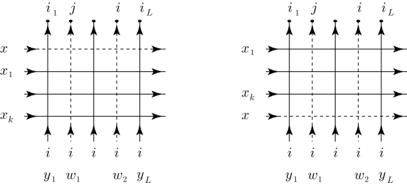
Figure 8. Lattice configurations.

The bonds on the lower boundary are assigned the (fixed and same) colour $i$, and the bonds on the upper boundary are assigned (fixed but varying) colours $i$, $j$, $i_{\ell}$, $\ell=1,\ldots,L$, $j<i$. We take the colours $s$ coming from the left boundary to be less than $i$, i.e. $s<i$, while the colours that remain unspecified (such as those on the bonds on the right boundary) can take any value that is allowed by colour conservation. If the top bond of the left-most vertical line has colour $i$, then all vertices on this vertical line are of type-$b$ and their weights factor out trivially.

We now consider the Higgsing of the dashed lines by imposing the condition (5.1), where, by the change of variables (B.2) this condition yields

(5.31) $$\textrm{A-type condition}:\ x_{k_{n}}^{(n)}=y_{L_{n-1}}^{(n)}-1\quad\textrm{and}\quad\textrm{B-type condition}:\ x_{k_{n}}^{(n)}=y_{L_{n}}^{(n)}$$

In other words, $a(x_{k_{n}}^{(n)},y_{L_{n-1}}^{(n)})=0$ and $b(x_{k_{n}}^{(n)},y_{L_{n}}^{(n)})=0$, respectively. For the above two lattice configurations, let us impose the A-type condition $a(x,w_{1})=0$ on the first dashed vertical line and the B-type condition $b(x,w_{2})=0$ on the second dashed vertical line. For the Higgsing, we further consider $x\to\infty$ limit corresponding to the decoupling of the vector multiplet scalar. With the above conditions, the dominant lattice configuration should be one with the minimal number of $c$ vertices on the dashed lines.

If the intersection of the horizontal dashed line and the vertical dashed line with top boundary colour $i$ is a $c$ vertex, then there are, at least, three (resp. two) $c$ vertices on the dashed lines for the left (resp. right) lattice configuration. To have the minimal number of $c$ vertices, this intersection should be an $a$ vertex by the B-type condition. In fact, in this case, the lattice configurations with minimal number of $c$ vertices are given in Figure 9.

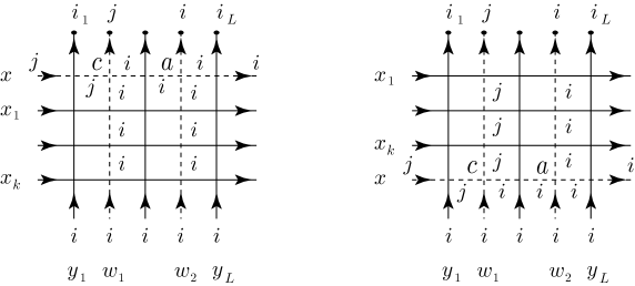
Figure 9. Higgsed lattice configurations.

Here, on the dashed lines, there is exactly one $c$ vertex at the intersection of the horizontal dashed line and the vertical dashed line with top boundary colour $j$. The other vertices on the dashed lines are also uniquely determined, where the left and right side boundary colours of the horizontal dashed line are fixed as $j$ and $i$, respectively. Note that without the second vertical dashed line with variable $w_{2}$, the lattice configuration on the dashed lines with a minimal number of $c$ vertex is not uniquely determined, and the Higgsing procedure for two vertical lines is inevitable.

Now we consider that the horizontal dashed lines are connected with other lattice configuration in Figure 10.

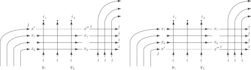
Figure 10. Higgsed lattice configurations connected with other lattices.

In this case, before taking the limit $x\to\infty$, we split this variable into three pieces $x$, $x^{\prime}$ and $x^{\prime\prime}$. As we will discuss in Section 6.3, the splitting of the variable $x$ is interpreted as the lattice version of a Hanany-Witten move. Further, we deform the lattice configuration by taking the decoupling limit $x^{\prime\prime}\to\infty$ to remove the horizontal line, with the variable $x^{\prime\prime}$ and colour $i$ at the two end boundaries, which uniquely results in no $c$ vertex .

Repeating this process, one can construct the $\mathfrak{su}(M+1)$ lattice configurations in Appendix B (e.g. see Figure 7) from the lattice configuration associated with the simple $A_{M}$ linear quiver in Figure 2.

6. The lattice versions of Higgsing and Hanany-Witten moves

6.1. Korepin’s specialization of parameters

A fundamental object in exact computations in spin-chain physics is the domain wall partition function (DWPF) introduced by Korepin, in the $\mathfrak{su}(2)$ spin-$\frac{1}{2}$ six-vertex model [27]. As explained in Appendix A, Korepin proposed a specialization of the parameters (the rapidities and the inhomogeneities) of the DWPF that leads to a recursion relation (and an initial condition) that completely determine it [27]. In [28], Izergin solved Korepin’s recursion relation and obtained a determinant expression for the DWPF (see Propositions A.3 and A.4).

6.2. Gaiotto and Koroteev’s specialization of parameters as a variation on Korepin’s

The specialization (5.1) of the parameters, used in the Higgsing procedure by Gaiotto and Koroteev, is a variation on Korepin’s, in the sense that it is essentially the same with two differences between them.

6.2.1. The first difference

Korepin’s derivation of the recursion relation requires one type of conditions, and can either, while the Higgsing procedure requires both as in (5.31).

In the case of domain wall boundary conditions, the DWPF is symmetric in the horizontal-line variables and also in the vertical-line variables, and one can choose the variables that one wishes to specialize to be those on lines on the boundaries of the (finite) lattice configuration on which the DWPF is defined. Once we do that, we have more information about the colours of the state variables on these lines, and only one condition is needed to derive the recursion relation.

In the case of Higgsing, when translated to the lattice, one deals with lattice configurations that correspond to the coordinate Bethe wavefunction which is not a symmetric function in the vertical-line (inhomogeneity) variables, one cannot (for general choices of the Higgsing parameters) associate the variables that one wishes to specialize to boundary lattice lines, and one requires (in general) two independent conditions. This makes the specialization of Gaiotto and Koroteev a more general version of Korepin’s.

6.2.2. The second difference

In Izergin-Korepin-type computations, one wishes to factor out the (finite) contributions of a single horizontal and a single vertical lattice line (rather than completely trivialize them), so the parameters that are identified by Korepin’s conditions are allowed to remain finite.

On the other hand, in the lattice version of Higgsing, one wishes to trivialize the contributions of a single horizontal and two vertical lattice lines, and this is achieved by identifying three parameters (using two conditions), then taking that parameter to infinity and normalizing appropriately. In the type-IIA/IIB brane realizations in Figure 4, this Higgsing procedure corresponds to Steps 1 and 2. This makes the specialization of Gaiotto and Koroteev a limiting case of Korepin’s.

6.3. The lattice version of the Hanany-Witten moves

One of the ingredients of the Higgsing of Gaiotto and Koroteev is a sequence of Hanany-Witten moves, in the sense that, in the type-IIA/IIB brane realizations in Figure 4, the transition from (anti-)bifundamental matter to new (anti-)fundamental matter is the result of Hanany-Witten moves and described by Step 3 [26, 16] . In Figure 5, the appearance (after Higgsing) of two pairs of fundamental and anti-fundamental matter from the pair of initial (before Higgsing) bifundamental and anti-bifundamental matter is the consequence of a sequence of Hanany-Witten moves. On the lattice side, following the splitting of the variable $x$ in Figure 10 and below, the disappearance of the initial horizontal-line parameter $x$, and the appearance of two new vertical-line parameters $x^{\prime}$ and $x^{\prime\prime}$, which is a re-assignment of what were (initially) horizontal-line variables as (new) vertical-line variables, is the lattice version of the Hanany-Witten move.

7. Remarks

7.1. Affinization

In [29], Bonelli, Sciarappa, Tanzini and Vasko studied connections between 4D $\mathcal{N}=2$ supersymmetric gauge theories and quantum integrable systems of the hydrodynamic type. In particular, the $\widehat{A}_{M}$ quiver gauge theory that plays a central role, and appears in Figure 1, in [29], is the affine version of the $A_{M}$ quiver gauge theory that plays a central role, and appears in Figure 1, in the present work. This leads us to expect that the present work has an affine extension along the lines of [29].

7.2. Quiver with orbifold defects

In Section 4, we considered a ${\mathbb{Z}}_{L}$ orbifold of the 2D gauge theory described by the $A_{M}$ quiver in Figure 2 and obtained the orbifold defect (4.19) labeled by the nested sequences (4.15). In [30], Bonelli, Fasola and Tanzini studied a class of 4D $A_{1}$ quiver gauge theories, with a codimension-2 surface defect, that supports nested instantons obtained by an orbifold and labeled by nested partitions. They discussed a 2D gauge theory described by a quiver that is different from that used in the present work, and that corresponds to the moduli space of nested instantons. It would be interesting to find the relation, if any, between the two constructions.

Appendix A The $\mathfrak{su}(2)$ six-vertex model partial domain wall partition function

We prove Proposition 4.5, to the effect that the partition function $\widehat{\mathcal{Z}}_{k}(\boldsymbol{u}_{k};\boldsymbol{m}_{L})$ in (4.11), constructed from the orbifold defect $\widehat{\psi}_{\boldsymbol{I}_{k}}^{(L)}(\boldsymbol{u}_{k};\boldsymbol{m}_{L})$ in (4.8), agrees with the $\mathfrak{su}(2)$ partial domain wall partition function (DWPF) of the rational six-vertex model.

Lemma A.1.

The orbifold defect $\widehat{\psi}_{\boldsymbol{I}_{k}}^{(L)}(\boldsymbol{u}_{k};\boldsymbol{m}_{L})$ and the partition function $\widehat{\mathcal{Z}}_{k}(\boldsymbol{u}_{k};\boldsymbol{m}_{L})$ are polynomials of degree $L-1$ in each $u_{a}$.

Proof.

We show that $\widehat{\mathcal{Z}}_{k}(\boldsymbol{u}_{k};\boldsymbol{m}_{L})$ is regular at $u_{A}=u_{B}$. Let $\widehat{\sigma}_{A,B}$ be an operator acting on functions of $\boldsymbol{u}_{k}$ which exchanges $u_{A}$ and $u_{B}$, and consider the defect $\omega_{\boldsymbol{I}_{k}}(\boldsymbol{u}_{k}):=\omega_{\boldsymbol{I}_{k}}^{(L)}(\boldsymbol{u}_{k};\boldsymbol{m}_{L})$ in (4.9). Symmetrizing in the variables ${\boldsymbol{u}_{k}}$, the pole at $u_{A}=u_{B}$, $A<B$, in $\omega_{\boldsymbol{I}_{k}}(\boldsymbol{u}_{k})$ cancels the corresponding pole in $\widehat{\sigma}_{A,B}\cdot\omega_{\boldsymbol{I}_{k}}(\boldsymbol{u}_{k})$. Therefore, $\omega_{\boldsymbol{I}_{k}}(\boldsymbol{u}_{k})+\widehat{\sigma}_{A,B}\cdot\omega_{\boldsymbol{I}_{k}}(\boldsymbol{u}_{k})$ has no poles at $u_{A}=u_{B}$, thus $\widehat{\psi}_{\boldsymbol{I}_{k}}^{(L)}(\boldsymbol{u}_{k};\boldsymbol{m}_{L})$ and $\widehat{\mathcal{Z}}_{k}(\boldsymbol{u}_{k};\boldsymbol{m}_{L})$ are regular at $u_{a}=u_{b}$, $a,b=1,\ldots,L$, and polynomials of degree $L-1$ in each $u_{a}$. ∎

Lemma A.2.

One can decouple the vector multiplet scalars by

(A.1) $$\widehat{\mathcal{Z}}_{k}(\boldsymbol{u}_{k};\boldsymbol{m}_{L})=\frac{1}{L-k}\lim_{u_{k+1}\to\infty}u_{k+1}^{1-L}\,\widehat{\mathcal{Z}}_{k+1}(\boldsymbol{u}_{k+1};\boldsymbol{m}_{L}),$$

and further,

(A.2) $$\widehat{\mathcal{Z}}_{k}(\boldsymbol{u}_{k};\boldsymbol{m}_{L})=\frac{1}{(L-k)!}\lim_{u_{k+1},\ldots,u_{L}\to\infty}\left\lgroup\prod_{a=k+1}^{L}u_{a}^{1-L}\right\rgroup\widehat{\mathcal{Z}}_{L}(\boldsymbol{u}_{L};\boldsymbol{m}_{L})$$

Proof.

The orbifold defect $\widehat{\psi}_{\boldsymbol{I}_{k}}^{(L)}(\boldsymbol{u}_{k};\boldsymbol{m}_{L})$ in (4.8) consists of $k!$ terms, and combining with the summation in (4.11), $\widehat{\mathcal{Z}}_{k}(\boldsymbol{u}_{k};\boldsymbol{m}_{L})$ contains $k!\times\binom{L}{k}=L!/(L-k)!$ terms in the summand. Comparing the summands on the both sides of (A.1), we find that the leading factor of $\widehat{\mathcal{Z}}_{k+1}(\boldsymbol{u}_{k+1};\boldsymbol{m}_{L})$ at $u_{k+1}\to\infty$ gives $(L-k)\,u_{k+1}^{L-1}\,\widehat{\mathcal{Z}}_{k}(\boldsymbol{u}_{k};\boldsymbol{m}_{L})$, and Equations (A.1) and (A.2) are obtained. ∎

Equation (A.2) states that by decoupling the vector multiplet scalars $u_{a}$, $a=k+1,\ldots,L$, from $\widehat{\mathcal{Z}}_{L}(\boldsymbol{u}_{L};\boldsymbol{m}_{L})=\widehat{\psi}_{\boldsymbol{I}_{L}}^{(L)}(\boldsymbol{u}_{L};\boldsymbol{m}_{L})$, one obtains $\widehat{\mathcal{Z}}_{k}(\boldsymbol{u}_{k};\boldsymbol{m}_{L})$. For $\widehat{\mathcal{Z}}_{L}(\boldsymbol{u}_{L};\boldsymbol{m}_{L})$, we have the following proposition.

Proposition A.3.

The partition function $\widehat{\mathcal{Z}}_{L}(\boldsymbol{u}_{L};\boldsymbol{m}_{L})$ satisfies the same four conditions that define the $\mathfrak{su}(2)$ DWPF in [27]. Namely, $\widehat{\mathcal{Z}}_{L}(\boldsymbol{u}_{L};\boldsymbol{m}_{L})$

• satisfies the initial condition $\widehat{\mathcal{Z}}_{1}(u;m)=1$,

• it is a polynomial of degree $L-1$ in each $u_{a}$,

• it is invariant under any permutations of $m_{i}$’s, and

• it satisfies the following recursion relation in $L$,

  (A.3) $$\widehat{\mathcal{Z}}_{L}(\boldsymbol{u}_{L};\boldsymbol{m}_{L})\Big{|}_{u_{L}=m_{L}-\frac{\gamma}{2}}=\prod_{a=1}^{L-1}\left\lgroup m_{L}-m_{a}-\gamma\right\rgroup\left\lgroup u_{a}-m_{L}-\frac{\gamma}{2}\right\rgroup\cdot\widehat{\mathcal{Z}}_{L-1}(\boldsymbol{u}_{L-1};\boldsymbol{m}_{L-1})$$

Proof.

Condition 1 follows from the definition of $\widehat{\mathcal{Z}}_{L}(\boldsymbol{u}_{L};\boldsymbol{m}_{L})$, and Condition 2 follows from Lemma A.1. To prove Condition 3, it is sufficient to show that $\omega_{\boldsymbol{I}_{L}}(\boldsymbol{u}_{L})+\widehat{\sigma}_{A,A+1}\cdot\omega_{\boldsymbol{I}_{L}}(\boldsymbol{u}_{L})$, in $\widehat{\mathcal{Z}}_{L}(\boldsymbol{u}_{L};\boldsymbol{m}_{L})$, is invariant under the permutation of $m_{A}$ and $m_{A+1}$, where $\omega_{\boldsymbol{I}_{L}}(\boldsymbol{u}_{L})=\omega_{\boldsymbol{I}_{L}}^{(L)}(\boldsymbol{u}_{L};\boldsymbol{m}_{L})$ is defined in (4.9). The point is that, once this is shown, then by symmetrizing $u_{A}$, $u_{A+1}$, and $u_{A+2}$ in $\omega_{\boldsymbol{I}_{L}}(\boldsymbol{u}_{L})$, the symmetrized function becomes invariant under permuting $m_{A}$, $m_{A+1}$, and $m_{A+2}$. In $\omega_{\boldsymbol{I}_{L}}(\boldsymbol{u}_{L})$, the factor that contains $u_{A}$ and $u_{A+1}$ is

(A.4) $$\prod_{a=A,A+1}^{L}\left\lgroup\prod_{i=1}^{a-1}\left\lgroup u_{a}-m_{i}-\frac{\gamma}{2}\right\rgroup\cdot\prod_{i=a+1}^{L}\left\lgroup u_{a}-m_{i}+\frac{\gamma}{2}\right\rgroup\right\rgroup\cdot\frac{u_{A,A+1}-\gamma}{u_{A,A+1}}\\ \times\prod_{a=1}^{A-1}\frac{\left\lgroup u_{a,A}-\gamma\right\rgroup\left\lgroup u_{a,A+1}-\gamma\right\rgroup}{u_{a,A}\,u_{a,A+1}}\cdot\prod_{a=A+2}^{L}\frac{\left\lgroup u_{A,a}-\gamma\right\rgroup\left\lgroup u_{A+1,a}-\gamma\right\rgroup}{u_{A,a}\,u_{A+1,a}}$$

Because the factor that contains $m_{A}$ and $m_{A+1}$, but does not contain $u_{A}$ and $u_{A+1}$,

(A.5) $$\prod_{i=A,A+1}^{L}\left\lgroup\prod_{a=A+2}^{L}\left\lgroup u_{a}-m_{i}-\frac{\gamma}{2}\right\rgroup\cdot\prod_{i=1}^{A-1}\left\lgroup u_{a}-m_{i}+\frac{\gamma}{2}\right\rgroup\right\rgroup,$$

is manifestly symmetric under the exchange of $m_{A}$ and $m_{A+1}$, in $\omega_{\boldsymbol{I}_{L}}(\boldsymbol{u}_{L})+\widehat{\sigma}_{A,A+1}\cdot\omega_{\boldsymbol{I}_{L}}(\boldsymbol{u}_{L})$, it is sufficient to consider the following factor in (A.4)

(A.6) $$\left\lgroup u_{A+1}-m_{A}-\frac{\gamma}{2}\right\rgroup\left\lgroup u_{A}-m_{A+1}+\frac{\gamma}{2}\right\rgroup\frac{u_{A,A+1}-\gamma}{u_{A,A+1}}$$

$$+\left\lgroup u_{A}-m_{A}-\frac{\gamma}{2}\right\rgroup\left\lgroup u_{A+1}-m_{A+1}+\frac{\gamma}{2}\right\rgroup\frac{u_{A,A+1}+\gamma}{u_{A,A+1}}$$

$$=-\left\lgroup m_{A}+m_{A+1}\right\rgroup\left\lgroup u_{A}+u_{A+1}\right\rgroup+2\left\lgroup m_{A}m_{A+1}+u_{A}u_{A+1}\right\rgroup+\frac{\gamma^{\,2}}{2}$$

Since this factor is symmetric under permuting $m_{A}$ and $m_{A+1}$, Condition 3 is proved. To prove Condition 4, we assign $u_{L}=m_{L}-\frac{\gamma}{2}$ in $\widehat{\mathcal{Z}}_{L}(\boldsymbol{u}_{L};\boldsymbol{m}_{L})$, the non-zero terms only come from $\mathop{\operatorname{Sym}}_{\boldsymbol{u}_{L-1}}\,\omega_{\boldsymbol{I}_{L}}(\boldsymbol{u}_{L})$, and by

(A.7) $$\widehat{\mathcal{Z}}_{L}(\boldsymbol{u}_{L};\boldsymbol{m}_{L})\Big{|}_{u_{L}=m_{L}-\frac{\gamma}{2}}=\\ \prod_{a=1}^{L-1}\left\lgroup u_{L}-m_{a}-\frac{\gamma}{2}\right\rgroup\left\lgroup u_{a}-m_{L}+\frac{\gamma}{2}\right\rgroup\,\frac{u_{a,L}-\gamma}{u_{a,L}}\bigg{|}_{u_{L}=m_{L}-\frac{\gamma}{2}}\times\widehat{\mathcal{Z}}_{L-1}(\boldsymbol{u}_{L-1};\boldsymbol{m}_{L-1}),$$

the recursion relation (A.3) is obtained. ∎

By induction in $L$, any function which satisfies the four conditions in Proposition A.3 is uniquely determined , and the partition function $\widehat{\mathcal{Z}}_{L}(\boldsymbol{u}_{L};\boldsymbol{m}_{L})$ agrees with Izergin’s determinant expression for the $\mathfrak{su}(2)$ DWPF [28] (see [31] for a review), which satisfies the same four conditions, as well as Kostov’s determinant expression [18, 19], which is equivalent to Izergin’s.

Proposition A.4.

The partition function $\widehat{\mathcal{Z}}_{L}(\boldsymbol{u}_{L};\boldsymbol{m}_{L})$ is an Izergin determinant [28]

(A.8) $$\widehat{\mathcal{Z}}_{L}(\boldsymbol{u}_{L};\boldsymbol{m}_{L})=\frac{\prod_{a,b=1}^{L}\left\lgroup u_{a}-m_{b}-\frac{\gamma}{2}\right\rgroup\left\lgroup u_{a}-m_{b}+\frac{\gamma}{2}\right\rgroup}{\prod_{a<b}^{L}u_{b,a}\,m_{a,b}}\\ \times\det\left\lgroup\frac{1}{\left\lgroup u_{a}-m_{b}-\frac{\gamma}{2}\right\rgroup\left\lgroup u_{a}-m_{b}+\frac{\gamma}{2}\right\rgroup}\right\rgroup_{a,b=1,\ldots,L},$$

or equivalently, a Kostov determinant [18, 19],

(A.9) $$\widehat{\mathcal{Z}}_{L}(\boldsymbol{u}_{L};\boldsymbol{m}_{L})=\frac{\prod_{a,b=1}^{L}\left\lgroup u_{a}-m_{b}+\frac{\gamma}{2}\right\rgroup}{\prod_{a<b}^{L}u_{b,a}}\\ \times\det\left\lgroup u_{a}^{b-1}\prod_{i=1}^{L}\frac{u_{a}-m_{i}-\frac{\gamma}{2}}{u_{a}-m_{i}+\frac{\gamma}{2}}-(u_{a}-\gamma)^{b-1}\right\rgroup_{a,b=1,\ldots,L},$$

which is an $\mathfrak{su}(2)$ DWPF, where $m_{a,b}=m_{a}-m_{b}$.

Proof of Proposition 4.5.

Taking the decoupling limit (A.2) in Proposition A.4, Proposition 4.5 is proved. ∎

Appendix B The $\mathfrak{su}(M+1)$ vertex model associated with the $A_{M}$ quiver

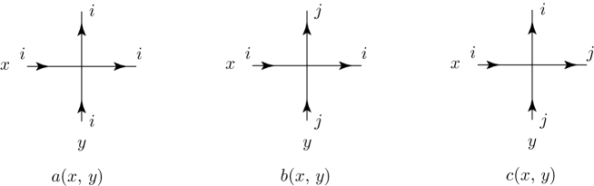
Figure 11. The non-zero vertex (Boltzmann) weights $w_{v}(x,y)$ (whose values are given in (B.4) in the case of the rational models, and in (B.5) in the case of the trigonometric models) that can assigned to a vertex $v$. The arrows indicate the directions of rapidity and inhomogeneity parameter flows, and the integers $i,j=1,\ldots,M+1$, $i\neq j$, are the state variables, or colours assigned to the bonds.

We describe the lattice configurations that represent the partition functions of the rational $\mathfrak{su}(M+1)$ vertex model that corresponds to the $\mathfrak{su}(M+1)$ XXX spin-chain with spins in the fundamental representation.

B.1. Notation

(B.1) $$\begin{split}&\boldsymbol{x}_{\boldsymbol{k}}^{M}=\{\boldsymbol{x}_{k_{1}}^{(1)},\ldots,\boldsymbol{x}_{k_{M}}^{(M)}\},\quad\boldsymbol{x}_{k_{\,p}}^{(p)}=\{x_{1}^{(p)},\ldots,x_{k_{\,p}}^{(p)}\},\\ &\boldsymbol{y}_{\boldsymbol{L}}^{M}=\{\boldsymbol{y}_{L_{1}}^{(1)},\ldots,\boldsymbol{y}_{L_{M}}^{(M)}\},\quad\boldsymbol{y}_{L_{\,p}}^{(p)}=\{y_{1}^{(p)},\ldots,y_{L_{\,p}}^{(p)}\},\quad p=1,\ldots,M,\end{split}$$

where $x_{a}^{(p)}$ and $y_{a}^{(p)}$ are the rapidities and inhomogeneities, respectively. The translation of the lattice parameters to the gauge theory parameters in Table 1 is

(B.2) $$x_{a}^{(p)}=u_{a}^{(p)}-\left\lgroup\frac{M-p+1}{2}\right\rgroup\,\gamma,\qquad y_{i}^{(p)}=m_{i}^{(p)}-\left\lgroup\frac{M-p}{2}\right\rgroup\,\gamma,\qquad\gamma=1$$

B.2. The vertex model

A square lattice representation of the rational $\mathfrak{su}(M+1)$ vertex model consists of horizontal lines that carry $x$-variables that flow from right to left, and vertical lines that carry $y$-variables that flow from bottom to top. The horizontal lines and the vertical lines intersect in vertices, and each vertex is connected to 4 line-segments that we call bonds. An internal bond is connected to two vertices and a boundary bond is connected to a single vertex. Each bond carries an arrow that indicates direction of the variable flow along it . Further, each bond carries a colour $i\in\{1,\ldots,M+1\}$, and colour is conserved , that is, if the colours on the bonds with incoming variable flows are $i$ and $j$, the colours on the bonds with outgoing variable flows are $k$ and $l$, then

(B.3) $$i+j=k+l$$

Given colour conservation (B.3), there are three types of vertices, type-$a$, type-$b$ and type-$c$, as in Figure 11, with vertex weights that depend (at most) on difference of variables

(B.4) $$a(x,y)=x-y+1,\quad b(x,y)=x-y,\quad c(x,y)=1$$

Remark B.1.

The vertex weights in the trigonometric $\mathfrak{su}(M+1)$ vertex model, which corresponds to the $\mathfrak{su}(M+1)$ XXZ spin-chain with spins in the fundamental representation, are

(B.5) $$a(x,y)=[x-y+1],\quad b(x,y)=[x-y],\quad c(x,y)=[1],$$

where $[x]=2\sinh(x/2)$.

We associate lattice configurations to the $A_{M}$ linear quiver in Figure 1, where $k_{\,p}\leq L_{\,p}+k_{p+1}$, $k_{M}\leq L_{M}$, $p=1,\ldots,M-1$, as follows. For the first node with $U(k_{1})$ gauge group, we associate one of the lattice configurations in Figure 12.

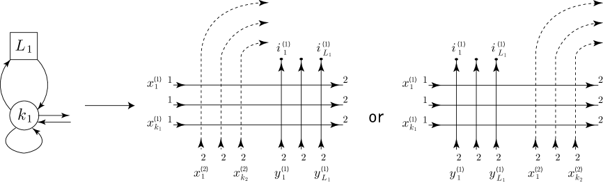
Figure 12. Two possible lattice configurations that can be associated with the first quiver node.

All bonds on the left boundary are assigned the (fixed and same) colour $1$, all bonds on the right and lower boundaries are assigned the (fixed and same) colour 2, and the $L_{1}$ bonds on the top boundary are assigned (fixed but varying) colours $i_{\ell}^{(1)}\in\{1,2\}$, $\ell=1,\ldots,L_{1}$. Each dashed line that carries a rapidity variable $x_{a}^{(2)}$ is connected with another dashed line that carries a rapidity variable $x_{a}^{(2)}$ associated with the second quiver node. For the $p$-th quiver node with a $U(k_{\,p})$ gauge group, $p=2,\ldots,M-1$, we associate one of the lattice configurations in Figure 13, where, each dashed line that carries a rapidity $x_{a}^{(p)}$ is connected with another dashed line that carries a rapidity variable $x_{a}^{(p)}$.

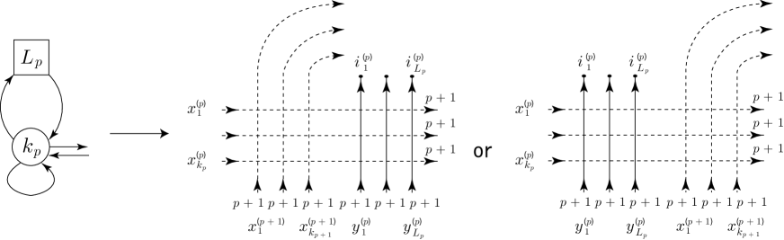
Figure 13. Two possible lattice configurations that can be associated with the $p$-th quiver node, where $p=2,\ldots,M-1$.

All bonds on the right boundary and on the lower boundary are assigned the (fixed and same) colour $p+1$, the $L_{\,p}$ bonds on the top boundary are assigned (fixed but varying) colours $i_{\ell}^{(L_{\,p})}\in\{1,\ldots,p+1\}$, $\ell=1,\ldots,L_{\,p}$, and we label the above left (resp. right) associated lattice configuration by $s_{p}=1$ (resp. $s_{p}=2$). For the $M$-th quiver node with $U(k_{M})$ gauge group, we associate the unique lattice configuration in Figure 14.

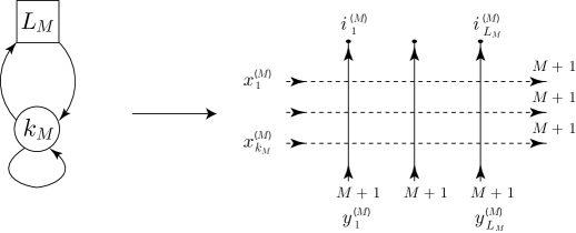
Figure 14. A lattice configuration associated with the $M$-th node.

The bonds on the right and lower boundaries are assigned the (fixed and same) colour $M+1$, and the $L_{M}$ bonds on the top boundary are assigned (fixed but varying) colours $i_{\ell}^{(L_{M})}\in\{1,\ldots,M+1\}$, $\ell=1,\ldots,L_{M}$. From colour conservation,

(B.6) $$\begin{split}&\sum_{p=1}^{M}\#_{1}\left\lgroup\boldsymbol{i}_{L_{\,p}}^{(p)}\right\rgroup=k_{1},\quad\sum_{p=q-1}^{M}\#_{q}\left\lgroup\boldsymbol{i}_{L_{\,p}}^{(p)}\right\rgroup=k_{q}-k_{q-1},\quad q=2,\ldots,M,\\ &\#_{M+1}\left\lgroup\boldsymbol{i}_{L_{M}}^{(M)}\right\rgroup=L_{M}-k_{M},\end{split}$$

where $\#_{q}(\boldsymbol{i}_{L_{\,p}}^{(p)})$ is the number of colours $q$ in the set $\boldsymbol{i}_{L_{\,p}}^{(p)}=\{i_{1}^{(p)},\ldots,i_{L_{\,p}}^{(p)}\}$. Examples of $\mathfrak{su}(2)$ and $\mathfrak{su}(3)$ lattice configurations are in Figures 3 and 7, respectively.

Definition B.2.

The partition function for the rational/trigonometric $\mathfrak{su}(M+1)$ lattice configuration associated with the $A_{M}$ linear quiver in Figure 1 is defined by

(B.7) $$\widehat{\psi}_{\mathrm{L},\boldsymbol{i}_{\boldsymbol{L}}^{M}}^{(\boldsymbol{S}|\boldsymbol{L})}\left\lgroup\boldsymbol{x}_{\boldsymbol{k}}^{M};\boldsymbol{y}_{\boldsymbol{L}}^{M}\right\rgroup=\sum_{{\boldsymbol{\sigma}}|_{\boldsymbol{i}_{\boldsymbol{L}}^{M}}}\prod_{v\in\boldsymbol{v}|_{\boldsymbol{\sigma}}}w_{v}\left\lgroup\mathsf{x}_{1}^{(v)},\mathsf{x}_{2}^{(v)}\right\rgroup,$$

where $\boldsymbol{i}_{\boldsymbol{L}}^{M}=\{\boldsymbol{i}_{L_{1}}^{(1)},\ldots,\boldsymbol{i}_{L_{M}}^{(M)}\}$ and $\boldsymbol{S}=\{s_{1},\ldots,s_{M-1}\}$, $s_{p}\in\{1,2\}$. ${\boldsymbol{\sigma}}|_{\boldsymbol{i}_{\boldsymbol{L}}^{M}}$ is a lattice configuration with fixed boundary colours $\boldsymbol{i}_{\boldsymbol{L}}^{M}$, and $\boldsymbol{v}|_{\boldsymbol{\sigma}}$ is the set of all vertices on the lattice with the lattice configuration ${\boldsymbol{\sigma}}$. $w_{v}(\mathsf{x}_{1}^{(v)},\mathsf{x}_{2}^{(v)})$ is the vertex weight on the vertex $v$ defined in Figure 11, where $\mathsf{x}_{1}^{(v)}$ and $\mathsf{x}_{2}^{(v)}$ are the corresponding variables.

References

- [1] N Nekrasov, Bethe States As Defects In Gauge Theories, (2013) http://scgp.stonybrook.edu/video_portal/video.php?id=1775
- [2] N Nekrasov, Bethe wavefunctions from gauged linear sigma models via Bethe/Gauge correspondence, (2014) http://scgp.stonybrook.edu/video_portal/video.php?id=1360
- [3] M Bullimore, H C Kim and T Łukowski, Expanding the Bethe/Gauge Dictionary, Journal of High Energy Physics 1711, 055 (2017), arXiv:1708.00445 [hep-th]
- [4] N A Nekrasov and S L Shatashvili, Supersymmetric vacua and Bethe ansatz, Nuclear Physics Proceedings Supplement 192-193, 91 (2009), arXiv:0901.4744 [hep-th]
- [5] N A Nekrasov and S L Shatashvili, Quantum integrability and supersymmetric vacua, Progress Theoretical Physics Supplement 177, 105 (2009), arXiv:0901.4748 [hep-th]
- [6] M Gaudin, The Bethe wavefunction, translated from French by J S Caux, Cambridge University Press, 2014, ISBN-10: 1107045851
- [7] F H L Essler, H Frahm, F Göhmann, A Klumper, and V E Korepin, The one-dimensional Hubbard model, Cambridge University Press, 2005, ISBN-10: 0521802628
- [8] C Closset, S Cremonesi and D S Park, The equivariant A-twist and gauged linear sigma models on the two-sphere, Journal of High Energy Physics 1506, 076 (2015), arXiv:1504.06308 [hep-th]
- [9] F Benini and A Zaffaroni, A topologically twisted index for three-dimensional supersymmetric theories, Journal of High Energy Physics 1507, 127 (2015), arXiv:1504.03698 [hep-th]
- [10] E Witten, Phases of theories in two-dimensions, Nuclear Physics B 403, 159 (1993), hep-th/9301042
- [11] D R Morrison and M R Plesser, Summing the instantons: Quantum cohomology and mirror symmetry in toric varieties, Nuclear Physics B 440, 279 (1995), hep-th/9412236
- [12] L C Jeffrey and F C Kirwan, Localization for nonabelian group actions, Topology 34, no. 2, 291-327 (1995), arXiv:alg-geom/9307001
- [13] M Brion and M Vergne, Arrangements of hyperplanes I: Rational functions and Jeffrey-Kirwan residue, Annales Scientifiques de l’École Normale Supérieure (4) 32, 715-741 (1999), arXiv:math/9903178 [math.DG]
- [14] A Szenes and M Vergne, Toric reduction and a conjecture of Batyrev and Materov, Inventiones mathematicae 158, no. 3, 453-495 (2004), arXiv:math/0306311 [math.AT]
- [15] F Benini, R Eager, K Hori and Y Tachikawa, Elliptic Genera of 2d Gauge Theories, Communications in Mathematical Physics 333, no. 3, 1241 (2015), arXiv:1308.4896 [hep-th]
- [16] D Gaiotto and P Koroteev, On Three Dimensional Quiver Gauge Theories and Integrability, Journal of High Energy Physics 1305, 126 (2013), arXiv:1304.0779 [hep-th]
- [17] O Foda and M Wheeler, Partial domain wall partition functions, Journal of High Energy Physics 1207, 186 (2012), arXiv:1205.4400 [math-ph]
- [18] I Kostov, Classical Limit of the Three-Point Function of Supersymmetric Yang-Mills Theory from Integrability, Physical Review Letters 108, 261604 (2012), arXiv:1203.6180 [hep-th]
- [19] I Kostov, Three-point function of semiclassical states at weak coupling, Journal of Physics A 45, 494018 (2012), arXiv:1205.4412 [hep-th]
- [20] M Mestyán, B Bertini, L Piroli and P Calabrese, Exact solution for the quench dynamics of a nested integrable system, Journal of Statistical Mechanics 1708, no. 8, 083103 (2017), arXiv:1705.00851 [cond-mat.stat-mech]
- [21] D Shenfeld, Abelianization of Stable Envelopes in Symplectic Resolutions, PhD thesis, Princeton, 2013
- [22] D Maulik and A Okounkov, Quantum Groups and Quantum Cohomology, arXiv:1211.1287 [math.AG]
- [23] R Rimanyi, V Tarasov and A Varchenko, Partial flag varieties, stable envelopes and weight functions, Quantum Topology 6, no. 2, 333-364 (2015), arXiv:1212.6240 [math.AG]
- [24] M Aganagic and A Okounkov, Quasimap counts and Bethe eigenfunctions, Moscow Mathematical Journal 17, no. 4, 565 (2017), arXiv:1704.08746 [math-ph]
- [25] O Foda and M Wheeler, Colour-independent partition functions in coloured vertex models, Nuclear Physics B 871, 330 (2013), arXiv:1301.5158 [math-ph]
- [26] A Hanany and E Witten, Type IIB superstrings, BPS monopoles, and three-dimensional gauge dynamics, Nuclear Physics B 492, 152 (1997), hep-th/9611230
- [27] V E Korepin, Calculation Of Norms Of Bethe Wave Functions, Communications in Mathematical Physics 86, 391 (1982)
- [28] A G Izergin, Partition function of the six-vertex model in a finite volume, Soviet Physics Doklady 32, 878 (1987)
- [29] G Bonelli, A Sciarappa, A Tanzini and P Vasko, Quantum Cohomology and Quantum Hydrodynamics from Supersymmetric Quiver Gauge Theories, Journal of Geometry and Physics 109, 3 (2016), arXiv:1505.07116 [hep-th]
- [30] G Bonelli, N Fasola and A Tanzini, Defects, nested instantons and comet shaped quivers, arXiv:1907.02771 [hep-th]
- [31] M A Wheeler, Free fermions in classical and quantum integrable models, PhD thesis, Melbourne, 2010, arXiv:1110.6703 [math-ph]