Robust and Resource Efficient Identification of Two Hidden Layer Neural Networks

Abstract

We address the structure identification and the uniform approximation of two fully nonlinear layer neural networks of the type $f(x)=1^{T}h(B^{T}g(A^{T}x))$ on $\mathbb{R}^{d}$, where $g=(g_{1},\dots,g_{m_{0}})$, $h=(h_{1},\dots,h_{m_{1}})$, $A=(a_{1}|\dots|a_{m_{0}})\in\mathbb{R}^{d\times m_{0}}$ and $B=(b_{1}|\dots|b_{m_{1}})\in\mathbb{R}^{m_{0}\times m_{1}}$, from a small number of query samples. The solution of the case of two hidden layers presented in this paper is crucial as it can be further generalized to deeper neural networks. We approach the problem by sampling actively finite difference approximations to Hessians of the network. Gathering several approximate Hessians allows reliably to approximate the matrix subspace $\mathcal{W}$ spanned by symmetric tensors $a_{1}\otimes a_{1},\dots,a_{m_{0}}\otimes a_{m_{0}}$ formed by weights of the first layer together with the entangled symmetric tensors $v_{1}\otimes v_{1},\dots,v_{m_{1}}\otimes v_{m_{1}}$, formed by suitable combinations of the weights of the first and second layer as $v_{\ell}=AG_{0}b_{\ell}/\|AG_{0}b_{\ell}\|_{2}$, $\ell\in[m_{1}]$, for a diagonal matrix $G_{0}$ depending on the activation functions of the first layer. The identification of the 1-rank symmetric tensors within $\mathcal{W}$ is then performed by the solution of a robust nonlinear program, maximizing the spectral norm of the competitors constrained over the unit Frobenius sphere. We provide guarantees of stable recovery under a posteriori verifiable conditions. Once the 1-rank symmetric tensors $\{a_{i}\otimes a_{i},i\in[m_{0}]\}\cup\{v_{\ell}\otimes v_{\ell},\ell\in[m_{1}]\}$ are computed, we address their correct attribution to the first or second layer ($a_{i}$’s are attributed to the first layer). The attribution to the layers is currently based on a semi-heuristic reasoning, but it shows clear potential of reliable execution. Having the correct attribution of the $a_{i},v_{\ell}$ to the respective layers and the consequent de-parametrization of the network, by using a suitably adapted gradient descent iteration, it is possible to estimate, up to intrinsic symmetries, the shifts of the activations functions of the first layer and compute exactly the matrix $G_{0}$. Eventually, from the vectors $v_{\ell}=AG_{0}b_{\ell}/\|AG_{0}b_{\ell}\|_{2}$’s and $a_{i}$’s one can disentangle the weights $b_{\ell}$’s, by simple algebraic manipulations. Our method of identification of the weights of the network is fully constructive, with quantifiable sample complexity, and therefore contributes to dwindle the black-box nature of the network training phase. We corroborate our theoretical results by extensive numerical experiments, which confirm the effectiveness and feasibility of the proposed algorithmic pipeline.

Keywords: deep neural networks, active sampling, exact identifiability, deparametrization, frames, nonconvex optimization on matrix spaces

1 Introduction

Deep learning is perhaps one of the most sensational scientific and technological developments in the industry of the last years. Despite the spectacular success of deep neural networks (NN) outperforming other pattern recognition methods, achieving even superhuman skills in some domains [12, 36, 58], and confirmations of empirical successes in other areas such as speech recognition [25], optical charachter recognition [8], games solution [44, 56], the mathematical understanding of the technology of machine learning is in its infancy. This is not only unsatisfactory from a scientific, especially mathematical point of view, but it also means that deep learning currently has the character of a black-box method and its success can not be ensured yet by a full theoretical explanation. This leads to lack of acceptance in many areas, where interpretability is a crucial issue (like security, cf. [10]) or for those applications where one wants to extract new insights from data [61].

Several general mathematical results on neural networks have been available since the 90’s [2, 17, 38, 39, 46, 47, 48], but deep neural networks have special features and in particular superior properties in applications that still can not be fully explained from the known results. In recent years, new interesting mathematical insights have been derived for undestanding approximation properties (expressivity) [27, 54] and stability properties [9, 68] of deep neural networks. Several other crucial and challenging questions remain open.

A fundamental one is about the number of required training data to obtain a good neural network, i.e., achieving small generalization errors for future data. Classical statistical learning theory splits this error into bias and variance and gives general estimations by means of the so-called VC-dimension or Rademacher complexity of the used class of neural networks [55]. However, the currently available estimates of these parameters [26] provide very pessimistic barriers in comparison to empirical success. In fact, the tradeoff between bias and variance is function of the complexity of a network, which should be estimated by the number of sampling points to identify it uniquely. Thus, on the one hand, it is of interest to know which neural networks can be uniquely determined in a stable way by finitely many training points. On the other hand, the unique identifiability is clearly a form of interpretability.
The motivating problem of this paper is the robust and resource efficient identification of feed forward neural networks. Unfortunately, it is known that identifying a very simple (but general enough) neural network is indeed NP-hard [7, 33]. Even without invoking fully connected neural networks, recent work [20, 41] showed that even the training of one single neuron (ridge function or single index model) can show any possible degree of intractability, depending on the distribution of the input. Recent results [3, 34, 42, 57, 52], on the other hand, are more encouraging, and show that minimizing a square loss of a (deep) neural network does not have in general or asymptotically (for large number of neurons) poor local minima, although it may retain the presence of critical saddle points.
In this paper we present conditions for a fully nonlinear two-layer neural network to be provably identifiable with a number of samples, which is polynomially depending on the dimension of the network. Moreover, we prove that our procedure is robust to perturbations. Our result is clearly of theoretical nature, but also fully constructive and easily implementable. To our knowledge, this work is the first, which allows provable de-parametrization of the problem of deep network identification, beyond the simpler case of shallow (one hidden) layer neural networks already considered in very recent literature [3, 32, 21, 34, 42, 43, 57, 52]. For the implementation we do not require black-box high dimensional optimization methods and no concerns about complex energy loss landscapes need to be addressed, but only classical and relatively simple calculus and linear algebra tools are used (mostly function differentiation and singular value decompositions). The results of this paper build upon the work [20, 21], where the approximation from a finite number of sampling points have been already derived for the single neuron and one-layer neural networks. The generalization of the approach of the present paper to networks with more than two hidden layers is suprisingly simpler than one may expect, and it is in the course of finalization [22], see Section 5 (v) below for some details.

1.1 Notation

Let us collect here some notation used in this paper. Given any integer $m\in\mathbb{N}$, we use the symbol $[m]:=\{1,2,\dots,m\}$ for indicating the index set of the first $m$ integers. We denote $B_{1}^{d}$ the Euclidean unit ball in $\mathbb{R}^{d}$, $\mathbb{S}^{d-1}$ the Euclidean sphere, and $\mu_{\mathbb{S}^{d-1}}$ is its uniform probability measure. We denote $\ell_{q}^{d}$ the $d$-dimensional Euclidean space endowed with the norm $\|x\|_{\ell_{q}^{d}}=\left(\sum_{j=1}^{d}|x_{j}|^{q}\right)^{1/q}$. For $q=2$ we often write indifferently $\|x\|=\|x\|_{2}=\|x\|_{\ell_{2}^{d}}$. For a matrix $M$ we denote $\sigma_{k}(M)$ its $k^{th}$ singular value. We denote $\mathbb{S}$ the sphere of symmetric matrices of unit Frobenius norm $\|\cdot\|_{F}$. The spectral norm of a matrix is denoted $\|\cdot\|$. Given a closed convex set $C$ we denote $P_{C}$ the orthogonal projection operator onto $C$ (sometimes we use such operators to project onto subspaces of $\mathbb{R}^{d}$ or subspaces of symmetric matrices or onto balls of such spaces). For vectors $x_{1},\dots,x_{k}\in\mathbb{R}^{d}$ we denote the tensor product $x_{1}\otimes\dots\otimes x_{k}$ as the tensor of entries $({x_{1}}_{i_{1}}\dots x_{k}{}_{i_{k}})_{i_{1},\dots,i_{k}}$. For the case of $k=2$ the tensor product $x\otimes y$ of two vectors $x,y\in\mathbb{R}^{d}$ equals the matrix $xy^{T}=(x_{i}y_{j})_{ij}$. For any matrix $M\in\mathbb{R}^{m\times n}$

$$\operatorname{vec}(M):=(m_{11},m_{21},\dots,m_{m1},m_{12},m_{22},\dots,m_{mn})^{T}\in\mathbb{R}^{mn},$$ (1)

is its vectorization, which is the vector created by the stacked columns of $M$.

1.2 From one artificial neuron to shallow, and deeper networks

1.2.1 Meet the neuron

The simplest artificial neural network $f:\Omega\subset\mathbb{R}^{d}\to\mathbb{R}$ is a network consisting of exactly one artificial neuron, which is modeled by a ridge-function (or single-index model) $f$ as

$$f(x)=\phi(a^{T}x+\theta)=g(a^{T}x),$$ (2)

where $g:\mathbb{R}\to\mathbb{R}$ is the shifted activation function $\phi(\cdot+\theta)$ and the vector $a\in\mathbb{R}^{d}$ expresses the weight of the neuron. Since the beginning of the 90’s [31, 30], there is a vast mathematical statistics literature about single-index models, which addresses the problem of approximating $a$ and possibly also $g$ from a finite number of samples of $f$ to yield an expected least-squares approximation of $f$ on a bounded domain $\Omega\subset\mathbb{R}^{d}$. Now assume for the moment that we can evaluate the network $f$ at any point in its domain; we refer to this setting as active sampling. As we aim at uniform approximations, we adhere here to the language of recent results about the sampling complexity of ridge functions from the approximation theory literature, e.g., [13, 20, 41]. In those papers, the identification of the neuron is performed by using approximate differentiation. Let us clarify how this method works as it will be of inspiration for the further developments below. For any $\epsilon>0$, points $x_{i}$, $i=1,\dots m_{\mathcal{X}}$, and differentiation directions $\varphi_{j}$, $j=1,\dots m_{\Phi}$ we have

$$\frac{f(x_{i}+\epsilon\varphi_{j})-f(x_{i})}{\epsilon}\approx\frac{\partial f(x_{i})}{\partial\varphi_{j}}=g^{\prime}(a^{T}x_{i})a^{T}\varphi_{j}.$$ (3)

Hence, differentiation exposes the weight of a neuron and allows to test it against test vectors $\varphi_{j}$. The approximate relationship (3) forms for every fixed index $i$ a linear system of dimensions $m_{\Phi}\times d$, whose unknown is $x^{*}_{i}=g^{\prime}(a^{T}x_{i})a$. Solving approximately and independently the systems for $i=1,\dots m_{\mathcal{X}}$ yields multiple approximations $\hat{a}=x^{*}_{i}/\|x^{*}_{i}\|_{2}\approx a$ of the weight, the most stable of them with respect to the approximation error in (3) is the one for which $\|x^{*}_{i}\|_{2}$ is maximal. Once $\hat{a}\approx a$ is learned then one can easily construct a function $\hat{f}(x)=\hat{g}(\hat{a}^{T}x)$ by approximating $\hat{g}(t)\approx f(\hat{a}t)$ on further sampling points. Under assumptions of smoothness of the activation function $g\in C^{s}([0,1])$, for $s>1$, $g^{\prime}(0)\neq 0$, and compressibility of the weight, i.e., $\|a\|_{\ell_{q}^{d}}$ is small for $0<q\leq 1$, then by using $L$ sampling points of the function $f$ and the approach sketched above, one can construct a function $\hat{f}(x)=\hat{g}(\hat{a}^{T}x)$ such that

$$\|f-\hat{f}\|_{C(\Omega)}\leq C\|a\|_{\ell_{q}^{d}}\left\{L^{-s}+\|g\|_{C^{s}([0,1])}\left(\frac{1+\log(d/L)}{L}\right)^{1/q-1/2}\right\}.$$ (4)

In particular, the result constructs the approximation of the neuron with an error, which has polynomial rate with respect to the number of samples, depending on the smoothness of the activation function and the compressibility of the weight vector $a$. The dependence on the input dimension is only logarithmical. To take advantage of the compressibility of the weight, compressive sensing [23] is a key tool to solve the linear systems (3). In [13] such an approximation result was obtained by active and deterministic choice of the input points $x_{i}$. In order to relax a bit the usage of active sampling, in the paper [20] a random sampling of the points $x_{i}$ has been proposed and the resulting error estimate would hold with high probability. The assumption $g^{\prime}(0)\neq 0$ is somehow crucial, since it was pointed out in [20, 41] that any level of tractability (polynomial complexity) and intractability (super-polynomial complexity) of the problem may be exhibited otherwise.

1.2.2 Shallow networks: the one-layer case

Combining several neurons leads to richer function classes [38, 39, 46, 47, 48]. A neural network with one hidden layer and one output is simply a weighted sum of neurons whose activation function only differs by a shift, i.e.,

$$f(x)=\sum^{m}_{i=1}b_{i}\phi(a_{i}^{T}x+\theta_{i})=\sum_{i=1}^{m}g_{i}(a_{i}^{T}x),$$ (5)

where $a_{i}\in\mathbb{R}^{m}$ and $b_{i},\theta_{i}\in\mathbb{R}$ for all $i=1,\dots,m$. Sometimes, it may be convenient below the more compact writing $f(x)=1^{T}g(A^{T}x)$ where $g=(g_{1},\dots,g_{m})$ and $A=[a_{1}|\dots|a_{m}]\in\mathbb{R}^{d\times m}$. Differently from the case of the single neuron, the use of first order differentiation

$$\nabla f(x)=\sum^{m}_{i=1}g_{i}^{\prime}(a_{i}^{T}x)a_{i}\in A=\operatorname{span}\left\{a_{1},\dots,a_{m}\right\},$$ (6)

may furnish information about $A=\operatorname{span}\left\{a_{1},\dots,a_{m}\right\}$ (active subspace identification [14, 15], see also [20, Lemma 2.1]), but it does not allow yet to extract information about the single weights $a_{i}$. For that higher order information is needed. Recent work shows that the identification of a network (5) can be related to tensor decompositions [1, 32, 21, 43]. As pointed out in Section 1.2.1 differentiation exposes the weights. In fact, one way to relate the network to tensors and tensor decompositions is given by higher order differentiation. In this case the tensor takes the form

$$D^{k}f(x)=\sum^{m}_{i=1}g_{i}^{(k)}(x)\underbrace{a_{i}\otimes\dots\otimes a_{i}}_{k-\text{times}},$$

which requires that the $g_{i}$’s are sufficiently smooth. In a setting where the samples are actively chosen, it is generally possible to approximate these derivatives by finite differences. However, even for passive sampling there are ways to construct similar tensors [32, 21], which rely on Stein’s lemma [59] or differentiation by parts or weak differentiation. Let us explain how passive sampling in this setting may be used for obtaining tensor representations of the network. If the probability measure of the sampling points $x_{i}$’s is $\mu_{X}$ with known (or approximately known [18]) density $p(x)$ with respect to the Lebesgue measure, i.e., $d\mu_{X}(x)=p(x)dx$, then we can approximate the expected value of higher order derivatives by using exclusively point evatuations of $f$. This follows from

$$\frac{1}{N}\sum^{N}_{i=1}f(x_{i})(-1)^{k}\frac{\nabla^{k}p(x_{i})}{p(x_{i})} \approx\int_{\mathbb{R}^{d}}f(x)(-1)^{k}\frac{\nabla^{k}p(x)}{p(x)}p(x)dx$$

$$=\int_{\mathbb{R}^{d}}\nabla^{k}f(x)d\mu_{X}(x)=\mathbb{E}_{x\sim\mu_{X}}[\nabla^{k}f(x)]$$

$$=\sum^{m}_{i=1}\left(\int_{\mathbb{R}^{d}}g^{(k)}(a_{i}^{T}x)d\mu_{X}(x)\right)\underbrace{a_{i}\otimes\dots\otimes a_{i}}_{k-\text{times}}.$$

In the work [32] decompositions of third order symmetric tensors ($k=3$) [1, 35, 51] have been used for the weights identification of one hidden layer neural networks. Instead, beyond the classical results about principal Hessian directions [37], in [21] it is shown that using second derivatives $(k=2)$ actually suffices and the corresponding error estimates reflect positively the lower order and potential of improved stability, see e.g., [16, 28, 29]. The main part of the present work is an extension of the latter approach and therefore we will give a short summary of it with emphasis on active sampling, which will be assumed in this paper as the sampling method. The first step of the approach in [21] is taking advantage of (6) to reduce the dimensionality of the problem from $d$ to $m$.

Reduction to the active subspace.

Before stating the core procedure, we want to introduce a simple and optional method, which can help to reduce the problem complexity in practice. Assume $f:\Omega\subset\mathbb{R}^{d}\to\mathbb{R}$ takes the form (5), where $d\geq m$ and that $a_{1},\dots,a_{m}\in\mathbb{R}^{d}$ are linearly independent. From a numerical perspective the input dimension $d$ of the network plays a relevant role in terms of complexity of the procedure. For this reason in [21] the input dimension is effectively reduced to the number of neurons in the first hidden layer. With this reasoning, in the sections that follow we also consider networks where the input dimension matches the number of neurons of the first hidden layer.

Assume for the moment that the active subspace $A=\operatorname{span}\left\{a_{1},\dots,a_{m}\right\}$ is known. Let us choose any orthonormal basis of $A$ and arrange it as the columns of a matrix $\hat{A}\in\mathbb{R}^{d\times m}$. Then

$$f(x)=f(P_{A}x)=f(\hat{A}\hat{A}^{T}x),$$

which can be used to define a new network

$$\hat{f}(y):=f(\hat{A}y):\mathbb{R}^{m}\to\mathbb{R}.$$ (7)

whose weights are $\alpha_{1}=\hat{A}^{T}a_{1},\dots,\alpha_{m}=\hat{A}^{T}a_{m}$, all the other parameters remain unchanged. Note that $\hat{A}\alpha_{i}=P_{A}a_{i}=a_{i}$, and therefore $a_{i}$ can be recovered from $\alpha_{i}$. In summary, if the active subspace of $f$ is approximately known, then we can construct $\hat{f}$, such that the identification of $f$ and $\hat{f}$ are equivalent. This allows us to reduce the problem to the identification of $\hat{f}$ instead of $f$, under the condition that we approximate $P_{A}$ well enough [21, Theorem 1.1]. As recalled in (6) we can produce easily approximations to vectors in $A$ by approximate first order differentiation of the original network $f$ and, in an ideal setting, generating $m$ linear independent gradients would suffices to approximate $A$. However, in general, there is no way to ensure a priori such linear independence and we have to account for the error caused by approximating gradients by finite differences. By suitable assumptions on $f$ (see the full rank condition on the matrix $J[f]$ defined in (8) below) and using Algorithm 1 we obtain the following approximation result.

Input: Given a shallow neural network $f$ as in (5), step-size of finite differences $\epsilon>0$, number of samples $m_{X}$

1 begin

2       Draw $x_{1},\dots,x_{m_{X}}$ uniformly from the unit sphere $\mathbb{S}^{d-1}$

3       Calculate the estimated gradients $\Delta_{\epsilon}f(x_{1}),\dots,\Delta_{\epsilon}f(x_{m_{X}})$ by first order finite differences with stepsize $\epsilon$.

4       Compute the singular value decomposition

$$\left(\Delta_{\epsilon}f(x_{1})\middle|\dots\middle|\Delta_{\epsilon}f(x_{m_{X}})\right)=\left(\begin{array}[]{lll}\hat{U}_{1}&\hat{U}_{2}\end{array}\right)\left(\begin{array}[]{ll}\hat{\Sigma}_{1}&0\\ 0&\hat{\Sigma}_{2}\\ \end{array}\right)\left(\begin{array}[]{l}\hat{V}_{1}^{T}\\ \hat{V}_{2}^{T}\end{array}\right),$$

where $\hat{\Sigma}_{1}$ contains the $m$ largest singular values. Set $P_{\hat{A}}=\hat{U}_{1}\hat{U}_{1}^{T}$.

5 end

6

Output: $P_{\hat{A}}$

Algorithm 1 Active subspace identification [21]

Theorem 1 ([21],Theorem 2.2).

Assume the vectors $(a_{i})_{i=1}^{m}$ are linear independent and of unit norm. Additionally, assume that the $g_{i}$’s are smooth enough. Let $P_{\hat{A}}$ be constructed as described in Algorithm 1 by sampling $m_{X}(d+1)$ values of $f$. Let $0<s<1$, and assume that the matrix

$$J[f] := \mathbb{E}_{X\sim\mu_{\mathbb{S}^{d-1}}}\nabla f(X)\otimes\nabla f(X)$$ (8)

$$= \int_{{\mathbb{S}}^{d-1}}\nabla f(x)\nabla f(x)^{T}d\mu_{{\mathbb{S}}^{d-1}}(x)$$

has full rank, i.e., its $m$-th singular value fulfills $\sigma_{m}\left(J[f]\right)\geq\alpha>0$. Then

$$\|P_{A}-P_{\hat{A}}\|_{F}\leq\frac{2C_{1}\epsilon m}{\sqrt{\alpha(1-s)}-C_{1}\epsilon m},$$

with probability at least $1-m\exp\Bigl{(}-\frac{m_{X}\alpha s^{2}}{2m^{2}C_{2}^{2}}\Bigr{)}$, where $C_{1},C_{2}>0$ are absolute constants depending on the smoothness of $g_{i}$’s.

Identifying the weights.

As clarified in the previous section we can assume from now on that $d=m$ without loss of generality. Let $f$ be a network of the type (5), with three times differentiable activation functions $(g_{i})_{i=1,\dots,m}$, and independent weights $(a_{i})_{i=1,\dots m}\in\mathbb{R}^{m}$ of unit norm. Then $f$ has second derivative

$$\nabla^{2}f(x)=\sum^{m}_{i=1}g_{i}^{\prime\prime}(a_{i}^{T}x)a_{i}\otimes a_{i}\in{\cal A}=\operatorname{span}\left\{a_{1}\otimes a_{1},\dots,a_{m}\otimes a_{m}\right\},$$ (9)

whose expression represents a non-orthogonal rank-1 decomposition of the Hessian. The idea is, first of all, to modify the network by an ad hoc linear transformation (withening) of the input

$$f(W^{T}x)=\sum_{i=1}^{m}g_{i}(a_{i}^{T}W^{T}x)$$ (10)

in such a way that $(Wa_{i}/\|Wa_{i}\|_{2})_{i=1,\dots,m}$ forms an orthonormal system. The computation of $W$ can be performed by spectral decomposition of any positive definite matrix

$$G\in\hat{\cal A}\approx{\cal A},\gamma I\preccurlyeq G.$$

In fact, from the spectral decomposition of $G=UDU^{T}$, we define $W=D^{-\frac{1}{2}}U^{T}$ (see [21, Theorem 3.7]). This procedure is called whitening and allows to reduce the problem to networks with nearly-orthogonal weights, and presupposes to have obtained $\hat{\cal A}\approx{\cal A}=\operatorname{span}\left\{a_{1}\otimes a_{1},\dots,a_{m}\otimes a_{m}\right\}$. By using (9) and a similar approach as Algorithm 1 (one simply substitutes there the approximate gradients with vectorized approximate Hessians), one can compute $\hat{\cal A}$ under the assumption that also the second order matrix

$$H[f] := \mathbb{E}_{X\sim\mu_{\mathbb{S}^{m-1}}}\operatorname{vec}(\nabla^{2}f(X))\otimes\operatorname{vec}(\nabla^{2}f(X))$$

$$= \int_{\mathbb{S}^{m-1}}\operatorname{vec}(\nabla^{2}f(x))\otimes\operatorname{vec}(\nabla^{2}f(x))d\mu_{\mathbb{S}^{m-1}}(x)$$

is of full rank, where $\operatorname{vec}(\nabla^{2}f(x))$ is the vectorization of the Hessian $\nabla^{2}f(x)$.

After whitening one could assume without loss of generality that the vectors $(a_{i})_{i=1,\dots m}\in\mathbb{R}^{m}$ are nearly orthonormal in the first place. Hence the representation (9) would be a near spectral decomposition of the Hessian and the components $a_{i}\otimes a_{i}$ would represent the approximate eigenvectors. However, the numerical stability of spectral decompositions is ensured only under spectral gaps [50, 4]. In order to maximally stabilize the approximation of the $a_{i}$’s, one seeks for matrices $M\in\hat{\cal A}$ with the maximal spectral gap between the first and second largest eigenvalues. This is achieved by the maximizers of the following nonconvex program

$$M=\arg\max\left\|{M}\right\|\quad\textrm{s.t.}\quad M\in\hat{\cal A},\quad\left\|{M}\right\|_{F}\leq 1,$$ (11)

where $\|\cdot\|$ and $\|\cdot\|_{F}$ are the spectral and Frobenius norms respectively. This program can be solved by a suitable projected gradient ascent, see for instance [21, Algorithm 3.4] and Algorithm 3 below, and any resulting maximizer has the eigenvector associated to the largest eigenvalue in absolute value close to one of the $a_{i}$’s. Once approximations $\hat{a}_{i}$ to all the $a_{i}$’s are retrieved, then it is not difficult to perform the identification of the activation functions $g_{i}$, see [21, Algorithm 4.1, Theorem 4.1]. The recovery of the network resulting from this algorithmic pipeline is summarized by the following statement.

Theorem 2 ([21],Theorem 1.2).

Let $f$ be a real-valued function defined on the neighborhood of $\Omega=B_{1}^{d}$, which takes the form

$$f(x)=\sum_{i=1}^{m}g_{i}(a_{i}\cdot x),$$

for $m\leq d$. Let $g_{i}$ be three times continuously differentiable on a neighborhood of $[-1,1]$ for all $i=1,\dots,m$, and let $\{a_{1},\dots,a_{m}\}$ be linearly independent. We additionally assume both $J[f]$ and $H[f]$ of maximal rank $m$. Then, for all $\epsilon>0$ (stepsize employed in the computation of finite differences), using at most $m_{\mathcal{X}}[(d+1)+(m+1)(m+2)/2]$ random exact point evaluations of $f$, the nonconvex program (11) constructs approximations $\{\hat{a}_{1},\dots,\hat{a}_{m}\}$ of the weights $\{a_{1},\dots,a_{m}\}$ up to a sign change for which

$$\bigg{(}\sum_{i=1}^{m}\|\hat{a}_{i}-a_{i}\|_{2}^{2}\bigg{)}^{1/2}\lesssim\varepsilon,$$ (12)

with probability at least $1-m\exp\Bigl{(}-\frac{m_{\mathcal{X}}c}{2\max\{C_{1},C_{2}\}^{2}m^{2}}\Bigr{)}$, for a suitable constant $c>0$ intervening (together with some fixed power of $m$) in the asymptotical constant of the approximation (12). Moreover, once the weights are retrieved one constructs an approximating function $\hat{f}:B_{1}^{d}\to\mathbb{R}$ of the form

$$\hat{f}(x)=\sum_{i=1}^{m}\hat{g}_{i}(\hat{a}_{i}\cdot x),$$

such that

$$\|f-\hat{f}\|_{C(\Omega)}\lesssim\epsilon.$$ (13)

While this result have been generalized to the case of passive sampling in [21] and through whitening allows for the identification of non-orthogonal weights, it is restricted to the case of $m\leq d$ and linearly independent weights $\{a_{i}:i=1,\dots,m\}$.

The main goal of this paper is generalizing this approach to account for both the identification of two fully nonlinear hidden layer neural networks and the case where $m>d$ and the weights are not necessarily nearly orthogonal or even linearly independent (see Remark 2 below).

1.2.3 Deeper networks: the two layer case

What follows further extends the theory discussed in the previous sections to a wider class of functions, namely neural networks with two hidden layers. By doing so, we will also address a relevant open problem that was stated in [21], which deals with the identification of shallow neural networks where the number of neurons is larger than the input dimension. First, we need a precise definition of the architecture of the neural networks we intend to consider.

Definition 3.

Let $0<m_{1}\leq m_{0}\leq d$, and $\{a_{1},\ldots,a_{m_{0}}\}\subset\mathbb{R}^{d}$, $\{b_{1},\ldots,b_{m_{1}}\}\subset\mathbb{R}^{m_{0}}$ be sets of unit vectors, and denote $A:=[a_{1}|\ldots|a_{m_{0}}]\in\mathbb{R}^{d\times m_{0}}$, $B:=[b_{1}|\ldots|b_{m_{1}}]\in\mathbb{R}^{m_{0}\times m_{1}}$. Let $g_{1},\ldots,g_{m_{0}}$ and $h_{1},\ldots,h_{m_{1}}$ be univariate functions, and denote $G_{0}=\operatorname{diag}\left(g_{1}^{\prime}(0),\ldots,g_{m_{0}}^{\prime}(0)\right)$. We define

$${\cal F}(d,m_{0},m_{1}):=\left\{f:\mathbb{R}^{d}\to\mathbb{R}:f(x)=\sum_{\ell=1}^{m_{1}}h_{\ell}\left(\sum_{i=1}^{m_{0}}b_{i\ell}g_{i}\left(a_{i}^{T}x\right)\right)\right\},$$ (14)

with $\{a_{1},\ldots,a_{m_{0}}\}\subset\mathbb{R}^{d}$, $\{b_{1},\ldots,b_{m_{1}}\}\subset\mathbb{R}^{m_{0}}$, $g_{1},\ldots,g_{m_{0}}$ and $h_{1},\ldots,h_{m_{1}}$ satisfying

1. $g_{i}^{\prime}(0)\neq 0\quad\forall i=1,\ldots,m_{0}$,

2. a frame condition for the system $\{a_{1},\ldots,a_{m_{0}},v_{1},\ldots,v_{m_{1}}\}$ with $v_{\ell}:=\frac{AG_{0}b_{\ell}}{\left\|{AG_{0}b_{\ell}}\right\|}$, i.e. there exist constants $c_{f},C_{F}>0$ such that

   $$c_{f}\left\|{x}\right\|^{2}\leq\sum\limits_{i=1}^{m_{0}}\left\langle x,a_{i}\right\rangle^{2}+\sum\limits_{\ell=1}^{m_{1}}\left\langle x,v_{\ell}\right\rangle^{2}\leq C_{F}\left\|{x}\right\|^{2},$$ (15)

   for all $x\in\mathbb{R}^{d}$,

3. the derivatives of $g_{i}$ and $h_{\ell}$ are uniformly bounded according to

   $$\quad\max\limits_{i=1,\ldots,m_{0}}\sup\limits_{t\in\mathbb{R}}\left|{g_{i}^{(k)}(t)}\right|\leq\kappa_{k},\quad\textrm{ and }\quad\max\limits_{i=1,\ldots,m_{1}}\sup\limits_{t\in\mathbb{R}}\left|{h_{\ell}^{(k)}(t)}\right|\leq\eta_{k},\quad k=0,1,2,3.$$ (16)

Sometimes it may be convenient below the more compact writing $f(x)=1^{T}h(B^{T}g(A^{T}x))$ where $g=(g_{1},\dots,g_{m_{0}})$, $h=(h_{1},\dots,h_{m_{1}})$. In the previous section we presented a dimension reduction that can be applied to one layer neural networks, and which can be useful to reduce the dimensionality from the input dimension to the number of neurons of the first layer. The same approach can be applied to networks defined by the class ${\cal F}(d,m_{0},m_{1})$. For the approximation error of the active subspace, we end up with the following corollary of Theorem 1.

Corollary 1 (cf. Theorem 1).

Assume that $f\in{\cal F}(d,m_{0},m_{1})$ and let $P_{\hat{A}}$ be constructed as described in Algorithm 1 by sampling $m_{X}(d+1)$ values of $f$. Let $0<s<1$, and assume that the $m_{0}$-th singular value of $J[f]$ fulfills $\sigma_{m_{0}}\left(J[f]\right)\geq\alpha>0$. Then we have

$$\lVert P_{A}-P_{\hat{A}}\rVert_{F}\leq\frac{2C_{3}\epsilon m_{0}m_{1}}{\sqrt{(1-s)\alpha}-C_{3}\epsilon m_{0}m_{1}},$$

with probability at least $1-m_{0}\exp(-\frac{s^{2}m_{x}\alpha}{2C_{4}m_{1}})$ and constants $C_{3},C_{4}>0$ that depend only on $\kappa_{j},\eta_{j}$ for $j=0,\dots,3$.

From now on we assume $d=m_{0}$.

2 Approximating the span of tensors of weights

In the one layer case, which was described earlier, the unique identification of the weights is made possible by constructing a matrix space whose rank-1 basis elements are outer products of the weight profiles of the network. This section illustrates the extension of this approach beyond shallow neural networks. Once again, we will make use of differentiation and overall there will be many parallels to the approach in [21]. However, the intuition behind the matrix space will be less straightforward, because we can not anymore directly express the second derivative of a two layer network as a linear combination of symmetric rank-1 matrices. This is due to the fact that the Hessian matrix of a network $f\in{\cal F}(m_{0},m_{0},m_{1})$ has the form

$$\nabla^{2}f(x)= \sum^{m_{1}}_{\ell=1}h_{\ell}^{\prime}(b_{\ell}^{T}g(A^{T}x))\sum_{i=1}^{m_{0}}b_{i\ell}g_{i}^{\prime\prime}(a_{i}^{T}x)a_{i}\otimes a_{i}$$

$$+ \sum^{m_{1}}_{\ell=1}\sum^{m_{0}}_{i,j=1}h_{\ell}^{\prime\prime}\left(b_{\ell}^{T}g(A^{T}x)\right)b_{i\ell}b_{j\ell}g_{i}^{\prime}(a_{i}^{T}x)g_{j}^{\prime}(a_{j}^{T}x)(a_{i}\otimes a_{j}+a_{j}\otimes a_{i})$$

Therefore, $\nabla^{2}f(x)\in\operatorname{span}\{a_{i}\otimes a_{j}+a_{j}\otimes a_{i}\;|\;i,j=1,\dots,m_{0}\}$, which has dimension $\frac{m_{0}(m_{0}+1)}{2}$ and is in general not spanned by symmetric rank-1 matrices. This expression is indeed quite complicated, due to the chain rule and the mixed tensor contributions, which are consequently appearing. At a first look, it would seem impossible to use a similar approach as the one for shallow neural networks recalled in the previous section. Nevertheless a relatively simple algebraic manipulation allows to recognize some useful structure: For a fixed $x\in\mathbb{R}^{m_{0}}$ we rearrange the expression as

$$\nabla^{2}f(x) =\sum^{m_{1}}_{\ell=1}h_{\ell}^{\prime}(b_{\ell}^{T}g(A^{T}x))\sum_{i=1}^{m_{0}}b_{i\ell}g_{i}^{\prime\prime}(a_{i}^{T}x)a_{i}\otimes a_{i}$$

$$+\sum^{m_{1}}_{\ell=1}h_{\ell}^{\prime\prime}\left(b_{\ell}^{T}g(A^{T}x)\right)\left[\sum^{m_{0}}_{i=1}b_{i\ell}g_{i}^{\prime}(a_{i}^{T}x)a_{i}\right]\otimes\left[\sum^{m_{0}}_{j=1}b_{j\ell}g_{j}^{\prime}(a_{j}^{T}x)a_{j}\right],$$

which is a combination of symmetric rank-1 matrices since $\sum^{m_{0}}_{j=1}b_{j\ell}g_{j}^{\prime}(a_{j}^{T}x)a_{j}\in\mathbb{R}^{m_{0}}$. We write the latter expression more compactly by introducing the notation

$$\nabla^{2}f(x)=\sum_{i=1}^{m_{0}}\gamma_{i}(x)a_{i}\otimes a_{i}+\sum^{m_{1}}_{\ell=1}\tau_{\ell}(x)v_{\ell}(x)\otimes v_{\ell}(x),$$ (17)

where $G_{x}=\operatorname{diag}\left(g_{1}^{\prime}(a_{1}^{T}x),\dots,g_{m_{0}}^{\prime}(a_{m_{0}}^{T}x)\right)\in\mathbb{R}^{m_{0}\times m_{0}}$ and

$$v_{\ell}(x) =AG_{x}b_{\ell}\in\mathbb{R}^{m_{0}} \text{for }\ell\in[m_{1}],$$ (18)

$$\gamma_{i}(x) =g_{i}^{\prime\prime}(a_{i}^{T}x)\sum^{m_{1}}_{\ell=1}h_{\ell}^{\prime}(b_{\ell}^{T}g(A^{T}x))b_{i\ell}\in\mathbb{R} \text{ for }i\in[m_{0}],$$ (19)

$$\tau_{\ell}(x) =h_{\ell}^{\prime\prime}\left(b_{\ell}^{T}g(A^{T}x)\right)\in\mathbb{R} \text{ for }\ell\in[m_{1}].$$ (20)

Figure 1: Illustration of the relationship between ${\cal W}$ (black line) and $\operatorname{span}\left\{\nabla^{2}f(x)\middle|x\in\mathbb{R}^{m_{0}}\right\}$ (light blue region) given by two non-linear cones that fan out from $\nabla^{2}f(0)$. There is no reason to believe that the these cones are symmetric around ${\cal W}$. The gray cones show the maximal deviation of $\hat{\cal W}$ from ${\cal W}$.

Let us now introduce the fundamental matrix space

$${\cal W}={\cal W}(f):=\operatorname{span}\left\{a_{1}\otimes a_{1},\dots,a_{m_{0}}\otimes a_{m_{0}},v_{1}\otimes v_{1},\dots,v_{m_{1}}\otimes v_{m_{1}}\right\},$$ (21)

where $a_{1},\dots,a_{m_{0}}$ are the weight profiles of the first layer and

$$v_{\ell}:=v_{\ell}(0)/\left\|{v_{\ell}(0)}\right\|_{2}=AG_{0}b_{\ell}/\|AG_{0}b_{\ell}\|_{2},$$

for all $\ell=1,\dots,m_{1}$ encode entangled information about $b_{1},\dots,b_{m_{1}}$. For this reason, we call the $v_{\ell}$’s entangled weights. Let us stress at this point that the definition and the constructive approximtion of the space ${\cal W}$ is perhaps the most crucial and relevant contribution of this paper. In fact, by inspecting carefully the expression (17), we immediately notice that $\nabla^{2}f(0)\in{\cal W}$, and also that the first sum in (17), namely $\sum_{i=1}^{m_{0}}\beta_{i}(x)a_{i}\otimes a_{i}$, lies in ${\cal W}$ for all $x\in\mathbb{R}^{m_{0}}$. Moreover, for arbitrary sampling points $x$, deviations of $\nabla^{2}f(x)$ from ${\cal W}$ are only due to the second term in (17). The intuition is that for suitable centered distributions of sampling points $x_{i}$’s so that $a_{j}^{T}x_{i}\approx 0$ and $G_{x_{i}}\approx G_{0}$, the Hessians $(\nabla^{2}f(x_{i}))_{i=1,\dots,m_{X}}$ will distribute themselves somehow around the space ${\cal W}$, see Figure 1 for a two dimensional sketch of the geometrical situation. Hence, we would attempt an approximation of ${\cal W}$ by PCA of a collection of such approximate Hessians. Practically, by active sampling (targeted evaluations of the network $f$) we first construct estimates $(\Delta_{\epsilon}^{2}f(x_{i}))_{i=1,\dots,m_{X}}$ by finite differences of the Hessian matrices $(\nabla^{2}f(x_{i}))_{i=1,\dots,m_{X}}$ (see Section 2.1), at sampling points $x_{1},\dots,x_{m_{X}}\in\mathbb{R}^{m}$ drawn independently from a suitable distribution $\mu_{X}$. Next, we define the matrix

$$\hat{W}=\left(\operatorname{vec}(\Delta_{\epsilon}^{2}f(x_{1})),\dots,\operatorname{vec}(\Delta_{\epsilon}^{2}f(x_{m_{X}}))\right),$$

whose columns are the vectorization of the approximate Hessians. Finally, we produce the approximation $\hat{\cal W}$ to ${\cal W}$ as the span of the first $m_{0}+m_{1}$ left singular vectors of the matrix $\hat{W}$. The whole procedure of calculating $\hat{\cal W}$ is given in Algorithm 2. It should be clear that the choice of $\mu_{X}$ plays a crucial role for the quality of this method. In the analysis that follows, we focus on distributions that are centered and concentrated. Figure 1 helps to form a better geometrical intuition of the result of the procedure. It shows the region covered by the Hessians, indicated by the light blue area, which envelopes the space ${\cal W}$ in a sort of nonlinear/nonconvex cone originating from $\nabla^{2}f(0)$. In general, the Hessians do not concentrate around ${\cal W}$ in a symmetric way, which means that the “center of mass” of the Hessians can never be perfectly aligned with the space ${\cal W}$, regardless of the number of samples. In this analogy, the center of mass is equivalent to the space estimated by Algorithm 2, which essentially is a non-centered principal component analysis of observed Hessian matrices. The primary result of this section is Theorem 4, which provides an estimate of the approximation error of Algorithm 2 depending on the subgaussian norm of the sample distribution $\mu_{X}$ and the number of neurons in the respective layers. More precisely, this result gives a precise worst case estimate of the error caused by the imbalance of mass. For reasons mentioned above, the error does not necessarily vanish with an increasing number of samples, but the probability under which the statement holds will tend to $1$. In Figure 1, the estimated region is illustrated by the gray cones that show the maximal, worst case deviation of $\hat{\cal W}$. One crucial condition for Theorem 4 to hold is that there exists an $\alpha>0$ such that

$$\sigma_{m_{0}+m_{1}}\left(\mathbb{E}_{X\sim\mu_{X}}\operatorname{vec}(\nabla^{2}f(X))\otimes\operatorname{vec}(\nabla^{2}f(X))\right)\geq\alpha.$$ (22)

This assumption makes sure that the space spanned by the observed Hessians has, in expectation, at least dimension $m_{0}+m_{1}$. Aside from this technical aspect this condition implicitly helps to avoid network configurations, which are reducible, for certain weights can not be recovered. For example, we can define a network in ${\cal F}(2,2,1)$ with weights given by

$$a_{1}=\begin{pmatrix}\frac{1}{\sqrt{2}}\\ \frac{1}{\sqrt{2}}\end{pmatrix},\,a_{2}=\begin{pmatrix}\frac{1}{\sqrt{2}}\\ -\frac{1}{\sqrt{2}}\end{pmatrix},b_{1}=\begin{pmatrix}1\\ 0\end{pmatrix}.$$

It is easy to see that $a_{2}$ will never be used during a forward pass through the network, which makes it impossible to recover $a_{2}$ from the output of the network.
In the theorem below and in the proofs that follow we will make use of the subgaussian norm $\left\|{\cdot}\right\|_{\psi_{2}}$ of a random variable. This quantity measures how fast the tails of a distribution decay and such a decay plays an important role in several concentration inequalities. More in general, for $p\geq 1$, the $\psi_{p}$-norm of a scalar random variable $Z$ is defined as

$$\left\|{Z}\right\|_{\psi_{p}}=\inf\left\{t>0:\mathbb{E}\exp(|Z/t|^{p})\leq 2\right\}.$$

For a random vector $X$ on $\mathbb{R}^{d}$ the $\psi_{p}$-norm is given by

$$\left\|{X}\right\|_{\psi_{p}}=\sup_{x\in\mathbb{S}^{d-1}}\left\|{\lvert\langle X,x\rangle\rvert}\right\|_{\psi_{p}}.$$

The random variables for which $\left\|{X}\right\|_{\psi_{1}}<\infty$ are called subexponential and those for which $\left\|{X}\right\|_{\psi_{2}}<\infty$ are called subgaussian. More in general, the Orlicz space $L_{\psi_{p}}=L_{\psi_{p}}(\Omega,\Sigma,\mathbb{P})$ consists of all real random variables $X$ on the probabillity space $(\Omega,\Sigma,\mathbb{P})$ with finite $\left\|{X}\right\|_{\psi_{p}}$ norm and its elements are called $p$-subexponential random variagles. Below, we mainly focus on subgaussian random variables. In particular, every bounded random variable is subgaussian, which covers all the cases we discuss in this work. We refer to [66] for more details. One example of a subgaussian distribution is the uniform distribution on the unit-sphere, which has subgaussian norm $\left\|{X}\right\|_{\psi_{2}}=\frac{1}{\sqrt{d}},X\sim\operatorname*{Unif}(\mathbb{S}^{d-1})$.

Input: Neural network $f$, number of estimated Hessians $m_{X}$, step-size of the finite difference approximation $\epsilon>0$, probability distribution $\mu_{X}$

1 begin

2       Draw $x_{1},\dots x_{m_{X}}$ independently from $\mu_{X}$

3       Calculate the matrix $M=\left(\operatorname{vec}(\Delta_{\epsilon}^{2}f(x_{1}))|\dots|\operatorname{vec}(\Delta_{\epsilon}^{2}f(x_{m_{X}}))\right)$

4       Set $U\Sigma V^{T}=\operatorname{SVD}(M)$

5       Denote by $U_{1}$ the first $m_{0}+m_{1}$ columns of $U$. $P_{\hat{\cal W}}=(u_{1}|\dots|u_{m_{0}+m_{1}})(u_{1}|\dots|u_{m_{0}+m_{1}})^{T}$

6      

7 end

8

Output: $P_{\hat{\cal W}}$

Algorithm 2 Approximating ${\cal W}$

Theorem 4.

Let $f\in{\cal F}(m_{0},m_{0},m_{1})$ be a neural network within the class described in Definition 3 and consider the space ${\cal W}$ as defined in (21). Assume that $\mu_{X}$ is a probability measure with ${\rm supp\ }(\mu_{X})\subset B^{m_{0}}_{1}$, $\mathbb{E}X=0$, and that there exists an $\alpha>0$ such that

$$\sigma_{m_{0}+m_{1}}\left(\mathbb{E}_{X\sim\mu_{X}}\operatorname{vec}(\nabla^{2}f(X))\otimes\operatorname{vec}(\nabla^{2}f(X))\right)\geq\alpha.$$ (23)

Then, for any $\epsilon>0$, Algorithm 2 returns a projection $P_{\hat{\cal W}}$ that fulfills

$$\left\|{P_{{\cal W}^{*}}-P_{\hat{\cal W}}}\right\|_{F}\leq\frac{\left(C_{\Delta}\epsilon m_{1}m_{0}^{\frac{3}{2}}+C\left\|{A}\right\|^{2}\left\|{B}\right\|^{2}\left\|{X}\right\|_{\psi_{2}}\sqrt{m_{1}\log(m_{0}+1)}\right)}{\sqrt{\frac{\alpha}{2}}-C_{\Delta}\epsilon m_{1}m_{0}^{\frac{3}{2}}},$$ (24)

for a suitable subspace ${\cal W}^{*}\subset{\cal W}$ (we can actually assume that ${\cal W}^{*}={\cal W}$ according to Remark 1 below) with probability at least

$$1-2e^{-c_{1}L_{1}m_{X}\min\left\{L_{1}m_{X},1\right\}}-(m_{0}+m_{1})e^{-L_{2}m_{X}}$$

where

$$L_{1} :=\left\|{X}\right\|^{2}_{\psi_{2}}\log(m_{0}+1)m_{1},L_{2}:=\alpha(8C_{1}\left\|{A}\right\|^{4}\left\|{B}\right\|^{4}m_{1})^{-1},$$

$c_{1},c_{2}$ are absolute constants and $C,C_{1},C_{\Delta}>0$ are constants depending on the constants $\kappa_{j},\eta_{j}$ for $j=0,\dots,3$.

Remark 1.

If $\epsilon>0$ is sufficiently small, due to (23) the space $\hat{\cal W}$ returned by Algorithm 2 has dimension $m_{0}+m_{1}$. If the error bound (24) in Theorem 4 is such that $\left\|{P_{{\cal W}^{*}}-P_{\hat{\cal W}}}\right\|_{F}<1$, then $\hat{\cal W}$ and ${\cal W}^{*}$ must have the same dimension. Moreover, ${\cal W}^{*}\subset{\cal W}$ and $\operatorname{dim}({\cal W})=m_{0}+m_{1}$ would necessarily imply that ${\cal W}={\cal W}^{*}$. Hence, for $\left\|{P_{{\cal W}^{*}}-P_{\hat{\cal W}}}\right\|_{F}<1$ and $\epsilon>0$ sufficiently small, we have ${\cal W}^{*}={\cal W}$.

As already mentioned above, for $\mu_{X}=\operatorname*{Unif}(\mathbb{S}^{m_{0}-1})$ we have $\left\|{X}\right\|_{\psi_{2}}=\frac{1}{\sqrt{m_{0}}}$. In this case the error bound 24 behaves like

$$\left\|{P_{{\cal W}}-P_{\hat{\cal W}}}\right\|_{F}\leq\mathcal{O}\left(\epsilon m_{1}m_{0}^{\frac{3}{2}}+\sqrt{\frac{m_{1}}{m_{0}}\log(m_{0}+1)}\right),$$

which is small for $\epsilon>0$ small and $m_{0}\gg m_{1}$. The latter condition seems favoring networks, for which the inner layer has a significantly larger number of neurons than the outer layer. This expectation is actually observed numerically, see Section 4. We have to add, though, that the parameter $\alpha>0$ that intervenes in the error bound (24) might also depend on $m_{0},m_{1}$ (as it is in fact an estimate of an $(m_{0}+m_{1})^{th}$ singular value as in (23)). Hence, the dependency on the network dimensions is likely more complex and depends on the interplay between the input distribution $\mu_{X}$ and the network architecture. In fact, at least judging from our numerical experiments, the error bound (24) is rather pessimistic and it certainly describes a worst case analysis. One more reason might be that some crucial estimates in its proof could be significantly improved. Another reason could be the rather great generality of the activation functions of the networks, which we analyze in this paper, as described in Definition 3. Perhaps the specific instances used in the numerical experiments are enjoying better identification properties.

2.1 Estimating Hessians of the network by finite differences

Before addressing the proof of Theorem 4, we give a precise definition of the finite differences we are using to approximate the Hessian matrices. Denote by $e_{i}$ the $i$-th Euclidean canonical basis vector in $\mathbb{R}^{d}$. We denote by $\Delta^{2}f(x):=\Delta_{\epsilon}^{2}f(x)$ the second order finite difference approximation of $\nabla^{2}f(x)$, given by

$$\Delta_{\epsilon}^{2}f(x)_{ij}:=\frac{f(x+\epsilon e_{i}+\epsilon e_{j})-f(x+\epsilon e_{i})-f(x+\epsilon e_{j})+f(x)}{\epsilon^{2}}$$ (25)

for $i,j=1,\dots,d=m_{0}$ and a step-size $\epsilon>0$. When it is not necessary, we will drop the step-size in the notation and simply write $\Delta^{2}f(x)$.

Lemma 5.

Let $f\in{\cal F}(m_{0},m_{0},m_{1})$ be a neural network. Further assume that $\Delta_{\epsilon}^{2}f(x)$ is constructed as in (25) for some $\epsilon>0$. Then we have

$$\sup_{x\in B^{d}_{1}}\lVert\nabla^{2}f(x)-\Delta^{2}_{\epsilon}(x)\rVert_{F}\leq C_{\Delta}\epsilon m_{1}m_{0}^{\frac{3}{2}},$$

where $C_{\Delta}>0$ is a constant depending on the constants $\kappa_{j},\eta_{j}$ for $j=0,\dots,3$.

For the proof of Lemma 5 we simply use the Lipschitz continuity of the functions $g,h$ and of their derivatives, and make use of $\left\|{a}\right\|_{2},\left\|{b}\right\|_{2}\leq 1$. The details can be found in the Appendix (Section A.1).

2.2 Span of tensors of (entangled) network weights: Proof of Theorem 4

The proof can essentially be divided into two separate bounds. Both will be addressed separately with the two lemmas below. For both lemmas we will assume that $X_{1},\dots,X_{m_{X}}\sim\mu_{X}$ independently and that ${\rm supp\ }(\mu_{X})\subseteq B^{m_{0}}_{1}$. Additionally, we define the random matrices

$$W :=(\operatorname{vec}(\nabla^{2}f(X_{1}))|\dots|\operatorname{vec}(\nabla^{2}f(X_{m_{X}}))),$$ (26)

$$\hat{W} :=(\operatorname{vec}(\Delta^{2}f(X_{1}))|\dots|\operatorname{vec}(\Delta^{2}f(X_{m_{X}})),$$ (27)

$$W^{*} :=(\operatorname{vec}(P_{{\cal W}}\nabla^{2}f(X_{1}))|\dots|\operatorname{vec}(P_{{\cal W}}\nabla^{2}f(X_{m_{X}}))),$$ (28)

where $P_{{\cal W}}$ denotes the orthogonal projection onto ${\cal W}$ (cf. (21)). For reader’s convenience, we recall here from (17) that the Hessian matrix of $f\in{\cal F}(m_{0},m_{0},m_{1})$ can be expressed as

$$\nabla^{2}f(x)=\sum_{i=1}^{m_{0}}\gamma_{i}(x)a_{i}\otimes a_{i}+\sum^{m_{1}}_{\ell=1}\tau_{\ell}(x)v_{\ell}(x)\otimes v_{\ell}(x),$$

where $\gamma_{i}(x),\tau_{\ell}(x),$ and $v_{\ell}(x)$ are introduced in (18) - (20). We further simplify this expression by introducing the notations

$$V_{x} =\left(v_{1}(x)|\dots|v_{m_{1}}(x)\right)=AG_{x}B,$$ (29)

$$\Gamma_{x} =\operatorname{diag}\left(\gamma_{1}(x),\dots,\gamma_{m_{0}}(x)\right),$$ (30)

$$T_{x} =\operatorname{diag}\left(\tau_{1}(x),\dots,\tau_{m_{1}}(x)\right).$$ (31)

which allow us to re-write (17) in terms of matrix multiplications

$$\nabla^{2}f(x)=A\Gamma_{x}A^{T}+V_{x}T_{x}V_{x}^{T}.$$ (32)

Lemma 6.

Let $f\in{\cal F}(m_{0},m_{0},m_{1})$ and let $\hat{W},W^{*}$ be defined as in (27)-(28), where $\mu_{X}$ is a subgaussian distribution with subgaussian norm $\left\|{X}\right\|_{\psi_{2}}$. Then the bound

$$\left\|{\hat{W}-W^{*}}\right\|_{F}\leq\sqrt{m_{X}}\left(C_{\Delta}\epsilon m_{1}m_{0}^{\frac{3}{2}}+C\left\|{A}\right\|^{2}\left\|{B}\right\|^{2}\left\|{X}\right\|_{\psi_{2}}\sqrt{m_{1}\log(m_{0}+1)}\right)$$

holds with probability at least

$$1-2\exp\left(-c_{1}\left\|{X}\right\|^{2}_{\psi_{2}}\log(m_{0}+1)m_{1}m_{X}\min\left(c_{2}\left\|{X}\right\|^{2}_{\psi_{2}}\log(m_{0}+1)m_{1}m_{X},1\right)\right),$$

where $c_{1},c_{2}>0$ are absolute constants and $C,C_{\Delta}>0$ depend only on the constants $\kappa_{j},\eta_{j}$ for $j=0,\dots,3$.

Proof.

By triangle inequality we get

$$\left\|{\hat{W}-W^{*}}\right\|_{F} \leq\left\|{\hat{W}-W}\right\|_{F}+\left\|{W^{*}-W}\right\|_{F}.$$ (33)

For the first term on the right hand side we can use the worst case estimate from Lemma 5, which yields

$$\left\|{\hat{W}-W}\right\|_{F}\leq\sqrt{m_{X}}\sup_{x\in B_{1}^{d}}\lVert\Delta^{2}f(x)-\nabla^{2}f(x)\rVert_{F}\leq\sqrt{m_{X}}C_{\Delta}\epsilon m_{1}m_{0}^{\frac{3}{2}}$$ (34)

for some constant $C_{\Delta}>0$. The second term in (33) can be bounded by (the explanation of the individual identities and estimates follows immediately below)

$$\left\|{W-W^{*}}\right\|_{F}^{2} =\left(\sum^{m_{X}}_{i=1}\left\|{\operatorname{vec}(\nabla^{2}f(X_{i}))-\operatorname{vec}(P_{{\cal W}}\nabla^{2}f(X_{i}))}\right\|_{2}^{2}\right)$$

$$=\sum_{i=1}^{m_{X}}\left\|{V_{X_{i}}T_{X_{i}}V_{X_{i}}^{T}-V_{0}T_{X_{i}}V_{0}^{T}}\right\|^{2}_{F}\leq\sum_{i=1}^{m_{X}}4\left\|{(V_{X_{i}}-V_{0})T_{X_{i}}V_{X_{i}}^{T}}\right\|_{F}^{2}$$

$$\leq 4\sum_{i=1}^{m_{X}}\left(\left\|{(V_{X_{i}}-V_{0})}\right\|\left\|{T_{X_{i}}}\right\|_{F}\left\|{V_{X_{i}}}\right\|\right)^{2}$$

$$\leq 4\left\|{A}\right\|^{4}\left\|{B}\right\|^{4}\sum^{m_{X}}_{i=1}\left(\left\|{G_{X_{i}}-G_{0}}\right\|\left\|{T_{X_{i}}}\right\|_{F}\left\|{G_{X_{i}}}\right\|\right)^{2}$$

$$\leq 4\left\|{A}\right\|^{4}\left\|{B}\right\|^{4}m_{1}\kappa_{1}^{2}\eta_{2}^{2}\sum^{m_{X}}_{i=1}\left(\left\|{G_{X_{i}}-G_{0}}\right\|\right)^{2}\leq 4\kappa_{1}^{2}\kappa_{2}^{2}\eta_{2}^{2}\left\|{A}\right\|^{4}\left\|{B}\right\|^{4}m_{1}\sum^{m_{X}}_{i=1}\left\|{A^{T}X_{i}}\right\|^{2}_{\infty}.$$

In the first two equalities we made use of the fact that $A\Gamma_{x}A^{T}\in{\cal W}$ and that by definition of an orthogonal projection $\left\|{V_{X_{i}}T_{X_{i}}V_{X_{i}}^{T}-P_{{\cal W}}V_{X_{i}}T_{X_{i}}V_{X_{i}}^{T}}\right\|_{F}\leq\left\|{V_{X_{i}}T_{X_{i}}V_{X_{i}}^{T}-V_{0}T_{X_{i}}V_{0}^{T}}\right\|_{F}$. The remaining inequalities follow directly from the submultiplicativity of $\left\|{\cdot}\right\|_{F}$ and $\left\|{\cdot}\right\|$ combined with the Lipschitz continuity of the activation functions and their derivatives (cf. (3) A3). Since $\left\|{a_{j}}\right\|\leq 1$, we can estimate the sub-exponential norm of $\left\|{A^{T}X_{i}}\right\|^{2}_{\infty}=\max_{1\leq j\leq m_{0}}\langle X_{i},a_{j}\rangle^{2}$ by

$$\left\|{\max_{1\leq j\leq m_{0}}\langle X_{i},a_{j}\rangle^{2}}\right\|_{\psi_{1}} \leq c_{1}\log(m_{0}+1)\max_{1\leq j\leq m_{0}}\left\|{\langle X_{i},a_{j}\rangle^{2}}\right\|_{\psi_{1}}$$

$$=c_{1}\log(m_{0}+1)\max_{1\leq j\leq m_{0}}\left\|{\langle X_{i},a_{j}\rangle}\right\|_{\psi_{2}}^{2}\leq c_{1}\log(m_{0}+1)\left\|{X}\right\|_{\psi_{2}}^{2},$$

for an absolute constant $c_{1}>0$, where we applied [65, Lemma 2.2.2] in the first inequality and used that $\left\|{Y}\right\|_{\psi_{2}}^{2}=\left\|{Y^{2}}\right\|_{\psi_{1}}$ for any scalar random variable $Y$ together with the fact that the subgaussian norm of a vector is defined by $\left\|{X}\right\|_{\psi_{2}}=\sup_{x\in\mathbb{S}^{d-1}}|\langle x,X\rangle|$ (cf. [66]). The random vectors $X_{i}\sim\mu_{X}$ are i.i.d., which allows us to drop the dependency on $i$ in the last step. The previous bound also guarantees a bound on the expectation, which is due to $\mathbb{E}[|Y|^{p}]\leq p!\left\|{Y}\right\|_{\psi_{1}}$ (cf. [65]), namely, for $p=1$ and $Y=\max_{1\leq j\leq m_{0}}\langle X,a_{j}\rangle^{2}$

$$\mathbb{E}\left[\max_{1\leq j\leq m_{0}}\langle X,a_{j}\rangle^{2}\right]\leq\left\|{\max_{1\leq j\leq m_{0}}\langle X_{i},a_{j}\rangle^{2}}\right\|_{\psi_{1}}\leq c_{1}\log(m_{0}+1)\left\|{X}\right\|_{\psi_{2}}^{2}.$$ (35)

Denote $Z_{i}:=\left\|{A^{T}X_{i}}\right\|^{2}_{\infty}$ for all $i=1,\dots,m_{X}$, then

$$\left\|{W-W^{*}}\right\|_{F}^{2} \leq 4\kappa_{1}^{2}\kappa_{2}^{2}\eta_{2}^{2}\left\|{A}\right\|^{4}\left\|{B}\right\|^{4}m_{1}\sum^{m_{X}}_{i=1}Z_{i}.$$ (36)

Therefore, applying the Bernstein inequality for sub-exponential random variables [66, Theorem 2.8.1] to the right sum in (36) yields

$$\left\|{W-W^{*}}\right\|_{F}^{2}\leq 4\kappa_{1}^{2}\kappa_{2}^{2}\eta_{2}^{2}\left\|{A}\right\|^{4}\left\|{B}\right\|^{4}(c_{1}m_{X}m_{1}\log(m_{0}+1)\left\|{X}\right\|_{\psi_{2}}^{2}+t),$$

with probability at least

$$1-2\exp\left(-c\min\left(\frac{t^{2}}{\sum_{i=1}^{m_{X}}\left\|{Z_{i}}\right\|^{2}_{\psi_{1}}},\frac{t}{\max_{i\leq m_{X}}\left\|{Z_{i}}\right\|_{\psi_{1}}}\right)\right)$$

$$=1-2\exp\left(-c\frac{t}{\left\|{X}\right\|^{2}_{\psi_{2}}}\min\left(\frac{t}{m_{X}\left\|{X}\right\|^{2}_{\psi_{2}}},1\right)\right),$$

for all $t\geq 0$ and an absolute constant $c>0$. Then, by choosing $t=c_{1}m_{X}m_{1}\log(m_{0}+1)\left\|{X}\right\|_{\psi_{2}}^{2}$ and $c_{2}=c\cdot c_{1}$, we get

$$\left\|{W-W^{*}}\right\|_{F}^{2}\leq 8\kappa_{1}^{2}\kappa_{2}^{2}\eta_{2}^{2}\left\|{A}\right\|^{4}\left\|{B}\right\|^{4}c_{1}m_{X}m_{1}\log(m_{0}+1)\left\|{X}\right\|_{\psi_{2}}^{2}$$ (37)

with probability at least

$$1-2\exp\left(-c_{2}\left\|{X}\right\|^{2}_{\psi_{2}}\log(m_{0}+1)m_{1}m_{X}\min\left(c_{1}\left\|{X}\right\|^{2}_{\psi_{2}}\log(m_{0}+1)m_{1}m_{X},1\right)\right).$$ (38)

From (33), combining (34) and (37) yields

$$\left\|{\hat{W}-W^{*}}\right\|_{F} \leq\sqrt{m_{X}}\sup_{x\in\mathbb{B}^{d}}\lVert\Delta^{2}f(x)-\nabla^{2}f(x)\rVert_{F}+\sqrt{8c_{1}}\kappa_{1}\kappa_{2}\eta_{2}\left\|{A}\right\|^{2}\left\|{B}\right\|^{2}\left\|{X}\right\|_{\psi_{2}}\sqrt{m_{X}m_{1}\log(m_{0}+1)}$$

$$\leq\sqrt{m_{X}}C_{\Delta}\epsilon m_{1}m_{0}^{\frac{3}{2}}+\sqrt{8c_{1}}\kappa_{1}\kappa_{2}\eta_{2}\left\|{A}\right\|^{2}\left\|{B}\right\|^{2}\left\|{X}\right\|_{\psi_{2}}\sqrt{m_{X}m_{1}\log(m_{0}+1)},$$

where we used Lemma 5 in the second inequality, and the results holds at least with the probability given as in (38). Setting $C:=\sqrt{8c_{1}}\kappa_{1}\kappa_{2}\eta_{2}>0$ finishes the proof. ∎

Lemma 7.

Let $X\in\mu_{X}$ be centered and subgaussian. Furthermore, assume that $f\in{\cal F}(m_{0},m_{0},m_{1})$ and that $\hat{W}$ is given by (27) with step-size $\epsilon>0$. If

$$\sigma_{m_{0}+m_{1}}\left(\mathbb{E}_{X\sim\mu_{X}}\operatorname{vec}(\nabla^{2}f(X))\otimes\operatorname{vec}(\nabla^{2}f(X))\right)\geq\alpha>0,$$

then we have

$$\sigma_{m_{0}+m_{1}}(\hat{W})\geq\sqrt{m_{X}}\left(\sqrt{\frac{\alpha}{2}}-C_{\Delta}\epsilon m_{1}m_{0}^{\frac{3}{2}}\right),$$

with probability at least $1-(m_{0}+m_{1})\exp\left(-\frac{m_{X}\alpha}{8C_{1}\left\|{A}\right\|^{4}\left\|{B}\right\|^{4}m_{1}}\right)$, where $C_{\Delta},C_{1}>0$ depend only on the constants $\kappa_{j},\eta_{j}$ for $j=0,\dots,3$.

Proof.

By Weyl’s inequality we obtain

$$\sigma_{m_{0}+m_{1}}(\hat{W})\geq\sigma_{m_{0}+m_{1}}(W)-\left\|{W-\hat{W}}\right\|\geq\sigma_{m_{0}+m_{1}}(W)-C_{\Delta}\epsilon m_{1}m_{0}^{\frac{3}{2}}.$$ (39)

For the first term of the right hand side we have $\sigma_{m_{0}+m_{1}}(W)^{2}=\sigma_{m_{0}+m_{1}}(WW^{T})$, which can be written as a sum of the outer products of the columns

$$\sigma_{m_{0}+m_{1}}(WW^{T}) =\sum_{i=1}^{m_{X}}\operatorname{vec}(\nabla^{2}f(X_{i}))\otimes\operatorname{vec}(\nabla^{2}f(X_{i})),$$

additionally, the matrices $\operatorname{vec}(\nabla^{2}f(X_{i}))\otimes\operatorname{vec}(\nabla^{2}f(X_{i}))$ are independent and positive definite random matrices. The Chernov bound for the eigenvalues for sums of random matrices, due to Gittens and Tropp [24] applied to the right hand side of the last equation yields the following lower bound:

$$\sigma_{m_{0}+m_{1}}\left(\sum_{i=1}^{m_{X}}\operatorname{vec}(\nabla^{2}f(X_{i}))\otimes\operatorname{vec}(\nabla^{2}f(X_{i}))\right)\geq tm_{X}\alpha\text{ for }t\in[0,1],$$ (40)

with probability at least

$$1-(m_{0}+m_{1})\exp\left(-(1-t)^{2}\frac{m_{X}\alpha}{2K}\right),$$

where we set $K=\max_{x\in B^{d}_{1}}\left\|{\operatorname{vec}(\nabla^{2}f(x))\otimes\operatorname{vec}(\nabla^{2}f(x))}\right\|$, which we wish to estimate more explicitly. First, we have to bound the norm of the Hessian matrices. Let $X\sim\mu_{X}$, then

$$\left\|{\nabla^{2}f(X)}\right\|_{F} \leq\sup_{x\in B_{1}^{d}}\left\|{\nabla^{2}f(x)}\right\|_{F}=\sup_{x\in\mathbb{B}^{d}}\left\|{A\Gamma_{x}A^{T}+V_{x}T_{x}V_{x}^{T}}\right\|_{F}$$

$$\leq\sup_{x\in\mathbb{B}^{d}}\left\|{A}\right\|^{2}\left(\kappa_{2}\lVert B\rVert\sqrt{\sum_{\ell=1}^{m_{1}}h^{\prime}_{\ell}(b_{\ell}^{T}g(A^{T}x+\theta))}+\left\|{B}\right\|^{2}\kappa_{1}^{2}\lVert\Gamma_{x}\rVert_{F}\right)$$

$$\leq\left\|{A}\right\|^{2}\left(\kappa_{2}\lVert B\rVert\eta_{2}\sqrt{m_{1}}+\left\|{B}\right\|^{2}\kappa_{1}^{2}\eta_{2}\sqrt{m_{1}}\right)\leq\sqrt{C_{1}}\left\|{A}\right\|^{2}\left\|{B}\right\|^{2}\sqrt{m_{1}},$$

for some constant $C_{1}>0$. Now we can further estimate $K$ by

$$K =\max_{x\in B_{1}^{d}}\left\|{\operatorname{vec}(\nabla^{2}f(x))\otimes\operatorname{vec}(\nabla^{2}f(x))}\right\|\leq\max_{x\in B_{1}^{d}}\left\|{\operatorname{vec}(\nabla^{2}f(x))\otimes\operatorname{vec}(\nabla^{2}f(x))}\right\|_{F}$$

$$\leq\max_{x\in B_{1}^{d}}\left\|{\nabla^{2}f(x)}\right\|_{F}^{2}\leq C_{1}\left\|{A}\right\|^{4}\left\|{B}\right\|^{4}m_{1}.$$

Finally, we can finish the proof by plugging the above into (39) and by setting $t=\frac{1}{2}$. ∎

Proof of Theorem 4.

The proof is a combination of the previous lemmas together with an application of Wedin’s bound [60, 67]. Given $\hat{W},W^{*}$, let $\hat{U}\hat{\Sigma}\hat{V}^{T},U^{*}\Sigma^{*}{V^{*}}^{T}$ be their respective singular value decompositions. Furthermore, denote by $\hat{U}_{1},U_{1}^{*}$ the matrices formed by only the first $m_{0}+m_{1}$ columns of $\hat{U},U^{*}$, respectively. According to this notation, Algorithm 2 returns the orthogonal projection $P_{\hat{\cal W}}=\hat{U}_{1}\hat{U}_{1}^{T}.$ We also denote by $P_{{\cal W}^{*}}$ the projection given by $P_{{\cal W}^{*}}=U_{1}^{*}{U_{1}^{*}}^{T}.$ Then we can bound the difference of the projections by applying Wedin’s bound

$$\left\|{P_{\hat{\cal W}}-P_{{\cal W}^{*}}}\right\|_{F}=\left\|{\hat{U}_{1}\hat{U}_{1}^{T}-U_{1}^{*}{U_{1}^{*}}^{T}}\right\|_{F}\leq\frac{2\left\|{\hat{W}-W^{*}}\right\|_{F}}{\bar{\alpha}},$$

as soon as $\bar{\alpha}>0$ satisfies

$$\bar{\alpha}\leq\min_{\begin{subarray}{c}1<j\leq m_{0}+m_{1}\\ m_{0}+m_{1}+1\leq k\end{subarray}}\lvert\sigma_{j}(\hat{W})-\sigma_{k}(W^{*})\rvert\text{ and }\bar{\alpha}\leq\min_{1\leq j\leq m_{0}+m_{1}}\sigma_{j}(\hat{W}).$$

Since ${\cal W}$ has dimension $m_{0}+m_{1}$, we have $\max_{k\geq m_{0}+m_{1}+1}\sigma_{k}(W^{*})=0$. Therefore the second inequality is equivalent to the first, and we can choose $\bar{\alpha}=\sigma_{m_{0}+m_{1}}(\hat{W})\leq\min_{1\leq j\leq m_{0}+m_{1}}\sigma_{j}(\hat{W})$. Thus, we end up with the inequality

$$\left\|{P_{\hat{\cal W}}-P_{{\cal W}^{*}}}\right\|_{F}\leq\frac{2\left\|{\hat{W}-W^{*}}\right\|_{F}}{\sigma_{m_{0}+m_{1}}(\hat{W})}.$$

Applying the union bound for the two events in Lemma 6 and Lemma 7 in combination with the respective inequalities yields

$$\left\|{P_{\hat{\cal W}}-P_{{\cal W}^{*}}}\right\|_{F}\leq\frac{\left(C_{\Delta}\epsilon m_{1}m_{0}^{\frac{3}{2}}+C\left\|{A}\right\|^{2}\left\|{B}\right\|^{2}\left\|{X}\right\|_{\psi_{2}}\sqrt{m_{1}\log(m_{0}+1)}\right)}{\sqrt{\frac{\alpha}{2}}-C_{\Delta}\epsilon m_{1}m_{0}^{\frac{3}{2}}}$$ (41)

with probability at least $1-2e^{\left(-c_{1}L_{1}m_{X}\min\left\{c_{2}L_{1}m_{X},1\right\}\right)}-(m_{0}+m_{1})e^{-L_{2}m_{X}}$, where

$$L_{1} :=\left\|{X}\right\|^{2}_{\psi_{2}}\log(m_{0}+1)m_{1},\quad,\quad L_{2}:=\frac{\alpha}{8C_{1}\left\|{A}\right\|^{4}\left\|{B}\right\|^{4}m_{1}},$$

and $C,C_{1},C_{\Delta},c_{1},c_{2}>0$ are the constants from the lemmas above. ∎

3 Recovery of individual (entangled) neural network weights

The symmetric rank-$1$ matrices $\{a_{i}\otimes a_{i}:i\in[m_{0}]\}\cup\{v_{\ell}\otimes v_{\ell}:\ell\in[m_{1}]\}$ made of tensors of (entangled) neural network weights are the spanning elements of ${\cal W}$, which in turn can be approximated by $\hat{\cal W}$ as has been proved above. In this section, we explain under which conditions it is possible to stably identify approximations to the network profiles $\{a_{i}:i\in[m_{0}]\}\cup\{v_{\ell}:\ell\in[m_{1}]\}$ by a suitable selection process, Algorithm 3.

To simplify notation, we drop the differentation between weights $a_{i}$ and $v_{\ell}$ and simply denote ${\cal W}=\left\{w_{1}\otimes w_{1},\ldots,w_{m}\otimes w_{m}\right\}$, where $m=m_{0}+m_{1}$, and every $w_{\ell}$ equals either one of the $a_{i}$’s or one of the $v_{\ell}$’s. Thus, $m$ may be larger than $d$. We also use the notations $W_{j}:=w_{j}\otimes w_{j}$, and $\hat{W}_{j}:=P_{\hat{\cal W}}(W_{j})$. Provided that the approximation error $\delta:=\left\|{P_{{\cal W}}-P_{\hat{\cal W}}}\right\|_{F}$ satisfies $\delta<1$ (cf. Theorem 4), $\{\hat{W}_{j}:j\in[m]\}$ is the image of a basis under a bijective map, and thus can be used as a basis for $\hat{\cal W}$ (see Lemma 25 in the Appendix). We quantify the deviation from orthonormality by $\nu:=C_{F}-1$, see (15). As an example of suitable frames, normalized tight frames achieve the bounds $c_{f}=C_{F}=m/d$ [5, Theorem 3.1], see also [11]. For instance, for such frames $m=\lceil 1.2d\rceil>d$ would allow for $\nu=0.2$. These finite frames are related to the Thomson problem of spherical equidistribution, which involves finding the optimal way in which to place $m$ points on the sphere $\mathbb{S}^{d-1}$ in $\mathbb{R}^{d}$ so that the points are as far away from each other as possible. We further note that if $0<\nu<1$ then $\{W_{j}:j\in[m]\}$ is a system of linearly independent matrices, hence a Riesz basis (see Lemma 23 and (68) in the Appendix). We denote the corresponding lower and upper Riesz constants by $c_{r},C_{R}$.
Finally, for any real, symmetric matrix $X$, we let $X=\sum_{j=1}^{d}\lambda_{j}(X)u_{j}(X)\otimes u_{j}(X)$ be the spectral decomposition ordered according to $\|X\|=\lambda_{1}(X)\geq\ldots\geq\lambda_{d}(X)$ (in case $\lambda_{1}(X)=-\|X\|$, we actually consider $-X$ instead of $X$). In the following we are able to provide in Theorem 8 general recovery guarantees of network weights provided by the eigenvector associated to the largest eigenvalue in absolute value of any suitable matrix $M\in\hat{\cal W}\cap\mathbb{S}$.

Remark 2.

The problem considered in this section is how to approximate the individual $w_{\ell}\otimes w_{\ell}$ within the space ${\cal W}$ or more precisely by using its approximation $\hat{\cal W}$. As the analysis below is completely unaware of how the space $\hat{\cal W}$ has been constructed, in particular it does not rely on the fact that it comes from second order differentiation of a two hidden layer network, here we are actually implicitly able of addressing also the problem of the identification of weights for one hidden layer networks (5) with a number $m$ of neurons larger than the input dimension $d$, which was left as an open problem from [21].

3.1 Recovery guarantees

The network profiles $\{w_{j},j\in[m]\}$ are (up to sign) uniquely defined by matrices $\{W_{j}:j\in[m]\}$ as they are precisely the eigenvectors corresponding to the unique nonzero eigenvalue. Therefore it suffices to recover $\{W_{j}:j\in[m]\}$, and we have to study when such matrices can be uniquely characterized within the matrix space ${\cal W}$ by their rank-$1$ property. Let us stress that this problem is strongly related to similar and very relevant ones appearing recently in the literature addressing nonconvex programs to identify sparse vectors and low-rank matrices in linear subspaces, see, e.g., in [45, 49]. In Appendix A.2 (Lemma 24 and Corollary 3) we prove that unique identification is possible if any subset of $\lceil m/2\rceil+1$ vectors of $\{w_{j}:j\in[m]\}$ is linearly independent, and that such subset linear independence is actually implied by the frame bounds (15) if $\nu=C_{F}-1<\lceil\frac{m}{2}\rceil^{-1}$. Unfortunately, this assumption seems a bit too restrictive in our scenario, hence we instead resort to a weaker and robust version given by the following result. In particular, we prove that any near rank-$1$ matrix in $\hat{\cal W}$ of unit Frobenius norm is not too far from one of the $W_{j}$’s, provided that $\delta$ and $\nu$ are small.

Theorem 8.

Let $M\in\hat{\cal W}\cap\mathbb{S}$ and assume $\max\{\delta,\nu\}\leq 1/4$. If $\lambda_{1}(M)>\max\{2\delta,\lambda_{2}(M)\}$ then

$$\min_{\begin{subarray}{c}j=1,\ldots,m,\\ s\in\{-1,1\}\end{subarray}}\left\|{sw_{j}-u_{1}(M)}\right\|\leq\sqrt{8}\frac{c_{r}^{-1/2}\sqrt{\nu}+\nu+2\delta}{\lambda_{1}(M)-\lambda_{2}(M)}.$$ (42)

Before proving Theorem 8 we need the following technical result.

Lemma 9.

For any $M=\sum_{j=1}^{m}\sigma_{j}\hat{W}_{j}\in\hat{\cal W}\cap\mathbb{S}$ with $\lambda_{1}(M)\geq\delta/(1-\delta)$ we have $\max_{i}\sigma_{i}\geq 0$.

Proof.

Assume, to the contrary, that $\max_{j}\sigma_{j}<0$, and denote $Z=\sum_{j=1}^{m}\sigma_{j}W_{j}$ with $M=P_{\hat{\cal W}}(Z)$. $Z$ is negative definite, since $v^{T}Zv=\sum_{j=1}^{m}\sigma_{j}\left\langle w_{j},v\right\rangle^{2}$, and $\sigma_{j}<0$ for all $i=1,\ldots,m$. Moreover, we have $\left\|{Z}\right\|_{F}\leq(1-\delta)^{-1}$ by Lemma 25, and thus we get a contradiction by

$$\frac{\delta}{1-\delta}\leq\lambda_{1}(M)\leq\lambda_{1}(Z)+\left\|{M-Z}\right\|_{F}<\left\|{M-Z}\right\|_{F}\leq\frac{\delta}{1-\delta}.$$

∎

Proof of Theorem 8.

Let $\lambda_{1}:=\lambda_{1}(M)$, $u_{1}:=u_{1}(M)$ for short in this proof. We can represent $M$ in terms of the basis elements of $\hat{\cal W}$ as $M=\sum_{j=1}^{m}\sigma_{j}\hat{W}_{j}$, and let $Z\in{\cal W}$ satisfy $M=P_{\hat{\cal W}}(Z)$. Furthermore, let $\sigma_{j^{*}}=\max_{j}\sigma_{j}\geq 0$ where the non-negativity follows from Lemma 9. Using $Z=\sum_{j=1}^{m}\sigma_{j}w_{j}\otimes w_{j}$ and $\left\|{Z}\right\|_{F}\leq(1-\delta)^{-1}$, we first notice that

$$\lambda_{1} =\left\langle M,u_{1}\otimes u_{1}\right\rangle=\left\langle Z,u_{1}\otimes u_{1}\right\rangle+\left\langle M-Z,u_{1}\otimes u_{1}\right\rangle$$ (43)

$$\leq\sum_{j=1}^{m}\sigma_{j}\left\langle w_{j},u_{1}\right\rangle^{2}+\left\|{M-Z}\right\|_{F}\leq\sigma_{j^{*}}C_{F}+2\delta\leq\sigma_{j^{*}}+\nu+2\delta,$$

and

$$\lambda_{1} =\left\langle M,u_{1}\otimes u_{1}\right\rangle\geq\max_{j}\left\langle Z,w_{j}\otimes w_{j}\right\rangle-2\delta\geq\sigma_{j^{*}}+\sum_{i\neq j^{*}}\sigma_{i}\left\langle w_{i},u_{1}\right\rangle^{2}-2\delta$$ (44)

$$\geq\sigma_{j^{*}}-\left\|{\sigma}\right\|_{\infty}\nu-2\delta\geq\sigma_{j^{*}}-2\nu-2\delta,$$

where we used $\left\|{\sigma}\right\|_{\infty}\leq(1-\delta)^{-1}(1-\nu)^{-1}\leq 2$ according to Lemma 26. Hence $\left|{\lambda_{1}-\sigma_{j^{*}}}\right|\leq 2\delta+2\nu$. Define now $Q:=\mathsf{Id}-u_{1}\otimes u_{1}$. Choosing $s\in\{-1,1\}$ so that $s\left\langle w_{j^{*}},u_{1}\right\rangle\geq 0$ we can bound the left hand side in (42) by

$$\left\|{sw_{j^{*}}-u_{1}}\right\|^{2} =2(1-\left\langle sw_{j^{*}},u_{1}\right\rangle)\leq 2(1-\left\langle w_{j^{*}},u_{1}\right\rangle^{2})=2\left\|{Qw_{j^{*}}}\right\|^{2}=2\left\|{QW_{j^{*}}}\right\|_{F}^{2}.$$

Viewing $W_{j^{*}}=w_{j^{*}}\otimes w_{j^{*}}$ as the orthogonal projection onto the eigenspace of the matrix $\lambda_{1}W_{j^{*}}$, corresponding to eigenvalues in $[\infty,\lambda_{1}]$, we can use Davis-Kahans Theorem in the version of [4, Theorem 7.3.1] to further obtain

$$\left\|{sw_{j^{*}}-u_{1}}\right\| \leq\sqrt{2}\left\|{QW_{j^{*}}}\right\|_{F}\leq\sqrt{2}\frac{\left\|{Q(\lambda_{1}W_{j^{*}}-M)W_{j^{*}}}\right\|_{F}}{\lambda_{1}-\lambda_{2}}\leq\sqrt{2}\frac{\left\|{(\lambda_{1}W_{j^{*}}-M)W_{j^{*}}}\right\|_{F}}{\lambda_{1}-\lambda_{2}}.$$ (45)

To bound the numerator, we first use $\left\|{Z-M}\right\|_{F}\leq\delta/(1-\delta)$ in the decomposition

$$\left\|{(\lambda_{1}W_{j^{*}}-M)W_{j^{*}}}\right\|_{F}\leq\left\|{(\lambda_{1}W_{j^{*}}-Z)W_{j^{*}}}\right\|_{F}+\left\|{Z-M}\right\|_{F}\leq\left\|{(\lambda_{1}W_{j^{*}}-Z)W_{j^{*}}}\right\|_{F}+\frac{\delta}{1-\delta},$$

and then bound the first term using $\left|{\lambda_{1}-\sigma_{j^{*}}}\right|\leq 2\delta+2\nu$ and the frame property (15) by

$$\left\|{(\lambda_{1}W_{j^{*}}-Z)W_{j^{*}}}\right\|_{F} =\left\|{(\lambda_{1}-\sigma_{j^{*}})W_{j^{*}}+\sum\limits_{j\neq j^{*}}\sigma_{j}(w_{j}\otimes w_{j})W_{j^{*}}}\right\|_{F}$$

$$\leq\left|{\lambda_{1}-\sigma_{j^{*}}}\right|+\left\|{\sum\limits_{j\neq j^{*}}\sigma_{j}\left\langle w_{j^{*}},w_{j}\right\rangle w_{j^{*}}\otimes w_{j}}\right\|_{F}\leq 2\delta+2\nu+\sum\limits_{j\neq j^{*}}\left|{\sigma_{j}}\right|\left|{\left\langle w_{j^{*}},w_{j}\right\rangle}\right|$$

$$\leq 2\delta+2\nu+\left\|{\sigma}\right\|_{2}\sqrt{\sum\limits_{j\neq j^{*}}\left\langle w_{j^{*}},w_{j}\right\rangle^{2}}\leq 2\delta+2\nu+\left\|{\sigma}\right\|_{2}\sqrt{\nu}.$$

Combining these estimates with (45) and $\delta/(1-\delta)\leq 2\delta$, we obtain

$$\left\|{sw_{j^{*}}-u_{1}(M)}\right\|\leq\sqrt{2}\frac{2\delta+2\nu+\left\|{\sigma}\right\|_{2}\sqrt{\nu}+2\delta}{\lambda_{1}-\lambda_{2}}=\sqrt{2}\frac{\left\|{\sigma}\right\|_{2}\sqrt{\nu}+2\nu+4\delta}{\lambda_{1}-\lambda_{2}}$$

The result follows since $\{w_{j}\otimes w_{j}:j\in[m]\}$ is a Riesz basis and thus $\left\|{\sigma}\right\|_{2}\leq c_{r}^{-1/2}\left\|{Z}\right\|_{F}\leq 2c_{r}^{-1/2}$. ∎

The preceding result provides recovery guarantees for network weights provided by the eigenvector associated to the largest eigenvalue in absolute value of any suitable matrix $M\in\hat{\cal W}\cap\mathbb{S}$. The estimate is inversely proportional to the spectral gap $\lambda_{1}(M)-\lambda_{2}(M)$. The problem then becomes the constructive identification of matrices $M$ belonging to $\hat{\cal W}\cap\mathbb{S}$, which simultaneously maximize the spectral gap. Inspired by the results in [21] we propose to consider the following nonconvex program as selector of such matrices

$$M=\arg\max\left\|{M}\right\|\quad\textrm{s.t.}\quad M\in\hat{\cal W},\quad\left\|{M}\right\|_{F}\leq 1.$$ (46)

By maximizing the spectral norm under a Frobenius norm constraint, a local maximizer of the program should be as nearly rank one as possible within a given neighborhood. Moreover, if rank one matrices exist in $\hat{\cal W}$, these are precisely the global optimizers.

3.2 A nonlinear program: properties of local maximizers of (46)

In this section we prove that, except for spurious cases, local maximizers of (46) are generically almost rank-$1$ matrices in $\hat{\cal W}$. In particular we show that local maximizers either satisfy $\left\|{M}\right\|^{2}\geq 1-c\delta-c^{\prime}\nu$, for some small constants $c,c^{\prime}$, implying near minimal rankness, or $\left\|{M}\right\|^{2}\leq c\delta+c^{\prime}\nu$, i.e., all eigenvalues of $M$ are small, the mentioned spurious cases. Before addressing these estimates, we provide a characterization of the first and second order optimality conditions for (46), see [21] and also [62, 63].

Theorem 10 (Theorem 3.4 in [21]).

Let $M\in\hat{\cal W}\cap\mathbb{S}$ and assume there exists a unique $i^{*}\in[d]$ satisfying $\left|{\lambda_{i^{*}}(M)}\right|=\left\|{M}\right\|$. If $M$ is a local maximizer (46) then it fulfills the stationary or first order optimality condition

$$u_{i^{*}}(M)^{T}Xu_{i^{*}}(M)=\lambda_{i^{*}}(M)\left\langle X,M\right\rangle$$ (47)

for all $X\in\hat{\cal W}$. A stationary point $M$ (in the sense that $M$ fulfills (47)) is a local maximizer of (46) if and only if for all $X\in\hat{\cal W}$

$$2\sum\limits_{i\neq i^{*}}\frac{(u_{i^{*}}(M)^{T}Xu_{k}(M))^{2}}{\left|{\lambda_{i^{*}}(M)-\lambda_{k}(M)}\right|}\leq\left|{\lambda_{i^{*}}(M)}\right|\left\|{X-\left\langle X,M\right\rangle M}\right\|_{F}^{2}.$$ (48)

Proof.

For simplicity we drop the argument $M$ in $\lambda_{i}$, $u_{i}$, and without loss of generality we assume $\lambda_{i^{*}}=\left\|{M}\right\|$, otherwise we consider $-M$. Following the analysis in [21], for $X\in\hat{\cal W}\cap\mathbb{S}$ we can consider the function

$$f_{X}(\alpha)=\frac{\left\|{M+\alpha X}\right\|}{\left\|{M+\alpha X}\right\|_{F}},$$

because $M$ is a local maximizer if and only if $\alpha=0$ is a local maximizer of $f_{X}$ for all $X\in\hat{\cal W}\cap\mathbb{S}$.

Let us consider $X\in\hat{\cal W}\cap\mathbb{S}$ with $X\perp M$ first. We note that the simplicity of $\lambda_{i^{*}}$ implies that there exist analytic functions $\lambda_{i^{*}}(\alpha)$ and $u_{i^{*}}(\alpha)$ with $(M+\alpha X)u_{i^{*}}(\alpha)=\lambda_{i^{*}}(\alpha)u_{i^{*}}(\alpha)$ for all $\alpha$ in a neighborhood around $0$ [40, 50]. Therefore we can use a Taylor expansion $\left\|{M+\alpha X}\right\|=\lambda_{i^{*}}+\lambda^{\prime}_{i^{*}}(0)\alpha+\lambda^{\prime\prime}_{i^{*}}(0)\alpha^{2}/2+{\cal O}(\alpha^{3})$ and combine it with $\left\|{M+\alpha X}\right\|_{F}=\sqrt{1+\alpha^{2}}=1-\alpha^{2}/2+{\cal O}(\alpha^{4})$ to get

$$f_{X}(\alpha)=\left(1-\alpha^{2}/2\right)\left(\lambda_{i^{*}}+\lambda^{\prime}_{i^{*}}(0)\alpha+\lambda^{\prime\prime}_{i^{*}}(0)\alpha^{2}/2\right)+{\cal O}(\alpha^{3})\quad\textrm{as $\alpha\rightarrow 0$. }$$

Differentiating once we get $f_{X}^{\prime}(0)=\lambda^{\prime}_{i^{*}}(0)$, hence $\alpha=0$ is a stationary point if and only if $\lambda^{\prime}_{i^{*}}(0)$ vanishes. Following the computations in [21], we find that $\lambda^{\prime}_{i^{*}}(0)=u_{i^{*}}(0)^{T}Xu_{i^{*}}(0)=0$, and thus (47) follows for any $X\perp M$. For general $X$, we split $X=\left\langle X,M\right\rangle M+X_{\perp}$, and get $u_{i^{*}}(0)^{T}Xu_{i^{*}}(0)=\left\langle X,M\right\rangle u_{i^{*}}(0)^{T}Mu_{i^{*}}(0)=\lambda_{i^{*}}(0)\left\langle X,M\right\rangle$.

For (48), we have to check additionally $f^{\prime\prime}_{X}(\alpha)\leq 0$. The second derivative of $f_{X}(\alpha)$ at zero is given by $f_{X}^{\prime\prime}(0)=\lambda^{\prime\prime}_{i^{*}}(0)-\lambda_{i^{*}}(0)$, hence the condition for attaining a local maximum is $\lambda^{\prime\prime}_{i^{*}}(0)\leq\lambda_{i^{*}}(0)$. Again, we can follow the computations in [21] to obtain

$$\lambda^{\prime\prime}_{i^{*}}(0)=2\sum_{i\neq i^{*}}\frac{(u_{i^{*}}^{T}(0)Xu_{k}(0))^{2}}{\left|{\lambda_{i^{*}}(0)-\lambda_{k}(0)}\right|},$$

and (48) follows immediately for any $X\perp M$, $\left\|{X}\right\|_{F}=1$. For general $X$ we decompose it into $X=\left\langle X,M\right\rangle M+X_{\perp}$. Since $u_{i^{*}}^{T}(0)Mu_{k}(0)=0$ for all $k\neq i^{*}$, we get

$$2\sum_{i\neq i^{*}}\frac{(u_{i^{*}}^{T}(0)\left(\left\langle X,M\right\rangle M+X_{\perp}\right)u_{k}(0))^{2}}{\left|{\lambda_{i^{*}}(0)-\lambda_{k}(0)}\right|}=2\left\|{X_{\perp}}\right\|_{F}^{2}\sum_{i\neq i^{*}}\frac{\left(u_{i^{*}}^{T}(0)\left(\frac{X_{\perp}}{\left\|{X_{\perp}}\right\|_{F}}\right)u_{k}(0)\right)^{2}}{\left|{\lambda_{i^{*}}(0)-\lambda_{k}(0)}\right|}\leq\lambda_{i^{*}}(0)\left\|{X_{\perp}}\right\|_{F}^{2},$$

and the result follows from $\left\|{X_{\perp}}\right\|_{F}=\left\|{X-\left\langle X,M\right\rangle M}\right\|_{F}$. ∎

For simplicity, we denote $u_{i}:=u_{i}(M)$ and $\lambda_{i}=\lambda_{i}(M)$ throughout the rest of this section. Moreover, we assume $M$ satisfies

1. $\lambda_{1}=\left\|{M}\right\|$ (this is without loss of generality because $-M$ and $M$ may be both local maximizers),

2. $\lambda_{1}>\lambda_{2}$ (this is a useful technical condition in order to use the second order optimality condition (48)).

To derive the bounds for $\lambda_{1}$, we establish an inequality $0\leq\lambda_{1}^{2}(\lambda_{1}^{2}-1)+c\delta+c^{\prime}\nu$, which implies that $\lambda_{1}^{2}(M)$ is either close to $0$ or close to $1$. A first ingredient for obtaining the inequality is

$$\left\|{\hat{W}_{j}u_{1}}\right\|_{2}^{2}\geq u_{1}^{T}\hat{W}_{j}u_{1}-2\delta=\lambda_{1}\left\langle\hat{W}_{j},M\right\rangle-2\delta,$$ (49)

where we used $\left|{\|\hat{W}_{j}u_{1}\|^{2}-u_{1}^{T}\hat{W}_{j}u_{1}}\right|\leq 2\delta$ in the inequality, see Lemma 26 in Appendix A.2, and (47) in the equality. The other useful technical estimate is provided in the following Lemma, which is proven by leveraging the second order optimality condition (48).

Lemma 11.

Assume that $M$ is a local maximizer satisfying (A1) and (A2) and let $\max\{\delta,\nu\}<1/4$. For any $X\in\hat{\cal W}$ with $\left\|{X}\right\|_{F}\leq 1$ we have

$$\left\|{Xu_{1}}\right\|_{2}^{2}\leq\lambda_{1}^{2}\frac{1+\left\langle X,M\right\rangle^{2}}{2}+5\delta+2\nu.$$ (50)

For the proof of Lemma 11 we need a lower bound for the smallest eigenvalue (see Appendix A.2 for the proof of Lemma 12).

Lemma 12.

Assume that $M$ is a stationary point of (46) satisfying (A1) and (A2). If $\max\{\delta,\nu\}<1/4$, then $\lambda_{D}\geq-2\delta\lambda_{1}^{-1}-8\delta-4\nu$.

Proof of Lemma 11.

We first use (47) and (48) to get

$$\frac{2}{\lambda_{1}-\lambda_{D}}\left(\left\|{Xu_{1}}\right\|_{2}^{2}-\lambda_{1}^{2}\left\langle X,M\right\rangle^{2}\right) =\frac{2}{\lambda_{1}-\lambda_{D}}\left(\left\|{Xu_{1}}\right\|_{2}^{2}-\left\langle Xu_{1},u_{1}\right\rangle^{2}\right)=\frac{2}{\lambda_{1}-\lambda_{D}}\sum\limits_{i=2}^{D}\left\langle Xu_{1},u_{k}\right\rangle^{2}$$

$$\leq 2\sum\limits_{i=2}^{D}\frac{(u_{1}^{T}Xu_{k})^{2}}{\lambda_{1}-\lambda_{k}}\leq\lambda_{1}\left\|{X-\left\langle X,M\right\rangle M}\right\|_{F}^{2},$$

and then rearrange the inequality to obtain

$$\left\|{Xu_{1}}\right\|_{2}^{2} \leq\frac{\lambda_{1}(\lambda_{1}-\lambda_{D})}{2}\left(\left\|{X}\right\|_{F}^{2}-\left\langle X,M\right\rangle^{2}\right)+\lambda_{1}^{2}\left\langle X,M\right\rangle^{2}\leq\frac{\lambda_{1}(\lambda_{1}-\lambda_{D})}{2}+\frac{\lambda_{1}(\lambda_{1}+\lambda_{D})}{2}\left\langle X,M\right\rangle^{2}$$

$$=\lambda_{1}^{2}\frac{1+\left\langle X,M\right\rangle^{2}}{2}-\lambda_{1}\lambda_{D}\frac{1-\left\langle X,M\right\rangle^{2}}{2}.$$

Using the lower bound for $\lambda_{D}$ from Lemma 12, and $\lambda_{1}\leq 1$, we get

$$\left\|{Xu_{1}}\right\|_{2}^{2} \leq\lambda_{1}^{2}\frac{1+\left\langle X,M\right\rangle^{2}}{2}+\lambda_{1}\left(2\delta\lambda_{1}^{-1}+8\delta+4\nu\right)\frac{1-\left\langle X,M\right\rangle^{2}}{2}$$

$$\leq\lambda_{1}^{2}\frac{1+\left\langle X,M\right\rangle^{2}}{2}+(10\delta+4\nu)\frac{1-\left\langle X,M\right\rangle^{2}}{2}=\lambda_{1}^{2}\frac{1+\left\langle X,M\right\rangle^{2}}{2}+5\delta+2\nu.$$

∎

By combining (49) and (50) the bounds for $\lambda_{1}$ follow.

Theorem 13.

Assume that $M$ is a local maximizer of (46) satisfying (A1) and (A2), and assume $38\delta+13\nu<1/4$. Then we have $\lambda_{1}^{2}\geq 1-38\delta-13\nu$ or $\lambda_{1}^{2}\leq 38\delta+13\nu.$

Proof.

Let $j^{*}=\arg\max_{j}\sigma_{j}$. We first note that we can assume $\sigma_{j^{*}}\geq 0$ without loss of generality by Lemma 9, since there is nothing to show if $\lambda_{1}\leq 2\delta$. Now we consider (49) and (50) for $X=\hat{W}_{j^{*}}$ to get the inequality

$$\phantom{or,equivalently,}\lambda_{1}^{2}\frac{1+\left\langle\hat{W}_{j^{*}},M\right\rangle^{2}}{2}+5\delta+2\nu\geq\lambda_{1}\left\langle\hat{W}_{j^{*}},M\right\rangle-2\delta,$$ (51)

$$\mbox{or, equivalently, }0\leq\lambda_{1}^{2}-1+\left(1-\lambda_{1}\left\langle\hat{W}_{j},M\right\rangle\right)^{2}+14\delta+4\nu$$

$$\mbox{or, equivalently, }0\leq\lambda_{1}^{2}-1+\left(1-\lambda_{1}\sigma_{j^{*}}\left\|{\hat{W}_{j}}\right\|_{F}^{2}+\lambda_{1}\left(\sigma_{j^{*}}\left\|{\hat{W}_{j}}\right\|_{F}^{2}-\left\langle\hat{W}_{j},M\right\rangle\right)\right)^{2}+14\delta+4\nu.$$

We separate two cases. In the first case we have $\sigma_{j^{*}}>1$, which implies $\langle\hat{W}_{j},M\rangle>1-5\delta-2\nu$ and thus $\langle W_{j},M\rangle>1-6\delta-2\nu$ by Lemma 26 and $\max\{\delta,\nu\}<1/4$. Since $\langle W_{j},M\rangle=w_{j}^{T}Mw_{j}$, this implies $\lambda_{1}>1-6\delta-2\nu$, i.e., the result is proven. We continue with the case $\sigma_{j^{*}}\leq 1$, which implies $\lambda_{1}\sigma_{j^{*}}\|\hat{W}_{j}\|_{F}^{2}\leq 1$. Using Lemma 26 to bound $\sigma_{j^{*}}\|\hat{W}_{j}\|_{F}^{2}-\langle\hat{W}_{j},M\rangle$, $\lambda_{1}<1$ and $\|\hat{W}_{j}\|_{F}^{2}\geq 1-2\delta$, the last inequality in (51) implies

$$0\leq\lambda_{1}^{2}-1+\left(1-\lambda_{1}\sigma_{j^{*}}+6\delta+2\nu\right)^{2}+14\delta+4\nu.$$ (52)

Furthermore, by following the computation we performed for (43), we get $\sigma_{j^{*}}\geq\lambda_{1}-\nu-2\delta$, and inserting it in (52) we obtain

$$0 \leq\lambda_{1}^{2}-1+\left(1-\lambda_{1}^{2}+8\delta+3\nu\right)^{2}+14\delta+4\nu,\mbox{ implying }0\leq\lambda_{1}^{2}\left(\lambda_{1}^{2}-1\right)+38\delta+13\nu.$$

Provided that $38\delta+13\nu<1/4$, this quadratic inequality (in the unknown $\lambda_{1}^{2}$) has solutions $\lambda_{1}^{2}\geq 1-38\delta-13\nu$, or $\lambda_{1}^{2}\leq 38\delta+13\nu$. ∎

3.3 Analysis of the projected gradient ascent iteration

In Section 3.2 we analyze local maximizers of (46) and show that there exist small constants $c,c^{\prime}$ such that either $\left\|{M}\right\|^{2}\geq 1-c\delta+c^{\prime}\nu$, or $\left\|{M}\right\|^{2}\leq c\delta+c^{\prime}\nu$. Therefore, a local maximizer of (46) is either almost rank-$1$, or it has its energy distributed across many eigenvalues. This criterion can be easily checked in practice, and therefore maximizing (46) is a suitable approach for finding near rank-$1$ matrices in $\hat{\cal W}$. In this section, we show how those individual symmetric rank-$1$ tensors can be approximated by a simple iterative algorithm, Algorithm 3, making exclusive use of the projection $P_{\hat{\cal W}}$. Algorithm 3 strives to solve the nonconvex program (46), by iteratively increasing the spectral norm of its iterations. Our approach is closely related to the projected gradient ascent iteration [21, Algorithm 4.1], but we introduce some modifications, in particular we exchange the order of the normalization and the projection onto $\hat{\cal W}$. The proof of convergence of [21, Algorithm 4.1] takes advantage of that different ordering of these operations to address the case where ${\cal W}$ is spanned by at most $m\leq d$ rank-$1$ matrices formed as tensors of nearly orthonormal vectors (after whitening). In fact, its analysis is heavily based on approximated singular value or spectral decompositions. Unfortunately in our case the decomposition ${M=\sum_{j=1}^{m}\sigma_{j}w_{j}\otimes w_{j}}$ does not approximate the singular value or spectral decomposition since the $w_{j}$’s are redundant (they form a frame) and therefore are not properly nearly orthonormal in the sense required in [21].

Algorithm 3 is based on the iterative application of the operator $F_{\gamma}$ defined by

$$F_{\gamma}(X):=P_{\mathbb{S}}\circ P_{\hat{\cal W}}(X+\gamma u_{1}(X)\otimes u_{1}(X)),$$ (53)

with $\gamma>0$ and $P_{\mathbb{S}}$ as the projection onto the sphere $\mathbb{S}=\{X:\left\|{X}\right\|_{F}=1\}$. The following Lemma shows that, if $\lambda_{1}(X)>0$, the operator $F_{\gamma}$ is well-defined, in the sense that it is a single-valued operator.

1

Input: $P_{\hat{\cal W}}$ with arbitrary basis $\{b_{i}\}_{i=1,\ldots,m}$, stepsize $\gamma>0$, number of iterations $J$

2

3begin

4      

5      Sample $g\sim{\cal N}(0,\mathsf{Id}_{m})$, and let $M_{0}:=P_{\mathbb{S}}(\sum_{i=1}^{m}g_{i}b_{i})$.

6      

7      If $\left\|{M_{0}}\right\|$ is not an eigenvalue, take $-M_{0}$ instead.

8      

9      for j = 1,…,J do

10            

11            $M_{j+1}=P_{\mathbb{S}}\circ P_{\hat{\cal W}}(M_{j}+\gamma u_{1}(M_{j})\otimes u_{1}(M_{j}))$.

12       end for

13      

14 end

15

Output: $u_{1}(M_{J})$

16

17

18

Algorithm 3 Approximating neural network profiles

Lemma 14.

Let $X\in\hat{\cal W}\cap\mathbb{S}$ with $\lambda_{1}(X)>0$ and $\gamma>0$. Then $\left\|{P_{\hat{\cal W}}(X+\gamma u_{1}(X)\otimes u_{1}(X))}\right\|_{F}^{2}=1+2\gamma\lambda_{1}(X)+\gamma^{2}\left\|{P_{\hat{\cal W}}(u_{1}(X)\otimes u_{1}(X))}\right\|_{F}^{2}$. In particular, $F_{\gamma}(X)$ is well-defined and can be explicitly expressed as

$$F_{\gamma}(X)=\frac{P_{\hat{\cal W}}(X+\gamma u_{1}(X)\otimes u_{1}(X))}{\left\|{P_{\hat{\cal W}}(X+\gamma u_{1}(X)\otimes u_{1}(X))}\right\|_{F}}.$$

Proof.

The result follows from $\left\langle X,P_{\hat{\cal W}}(u_{1}(X)\otimes u_{1}(X))\right\rangle=\lambda_{1}(X)$ and computing explicitly the squared norm $\left\|{P_{\hat{\cal W}}(X+\gamma u_{1}(X)\otimes u_{1}(X))}\right\|_{F}^{2}$. ∎

We analyze next the sequence $(M_{j})_{j\in\mathbb{N}}$ generated by Algorithm 3. We show that $(\lambda_{1}(M_{j}))_{j\in\mathbb{N}}$ is a strictly monotone increasing sequence, converging to a well-defined limit $\lambda_{\infty}=\lim_{j\rightarrow\infty}\lambda_{1}(M_{j})$, and, if $\lambda_{1}(M_{j})>1/\sqrt{2}$ for some $j$, all convergent subsequences of $(M_{j})_{j\in\mathbb{N}}$ converge to fixed points of $F_{\gamma}$. Moreover, we prove that such fixed points satisfy (47), and are thus stationary points of (46). We begin by providing two equivalent characterizations of (47).

Lemma 15.

For $M\in\hat{\cal W}$ and $c\neq 0$ we have

$$v^{T}Xv=c\left\langle X,M\right\rangle\quad\textrm{ for all }X\in\hat{\cal W}\quad\textrm{ if and only if }\quad M=c^{-1}P_{\hat{\cal W}}(v\otimes v).$$

Proof.

Assume that $v^{T}Xv=c\left\langle X,M\right\rangle$ for all $X$. We notice that the assumption is equivalent to $\left\langle X,v\otimes v-cM\right\rangle=0$ for all $X\in\hat{\cal W}$. Therefore $P_{\hat{\cal W}}(v\otimes v-cM)=0$, and the result follows from $M\in\hat{\cal W}$. In the case where $M=c^{-1}P_{\hat{\cal W}}(v\otimes v)$, we compute $c\left\langle X,M\right\rangle=\left\langle X,P_{\hat{\cal W}}(v\otimes v)\right\rangle=v^{T}Xv$ since $X\in\hat{\cal W}$. ∎

Lemma 16.

Let $X\in\hat{\cal W}\cap\mathbb{S}$. We have $\left\|{P_{\hat{\cal W}}(u_{j}(X)\otimes u_{j}(X))}\right\|_{F}\geq\left|{\lambda_{j}(X)}\right|$ with equality if and only if $X=\lambda_{j}(X)^{-1}P_{\hat{\cal W}}(u_{j}(X)\otimes u_{j}(X))$.

Proof.

We drop the argument $X$ for $\lambda_{j}(X)$ and $u_{j}(X)$ for simplicity. We first calculate

$$\left\|{P_{\hat{\cal W}}(u_{j}\otimes u_{j})}\right\|_{F}=\left\|{P_{\hat{\cal W}}(u_{j}\otimes u_{j})}\right\|_{F}\left\|{X}\right\|_{F}\geq\left|{\left\langle P_{\hat{\cal W}}(u_{j}\otimes u_{j}),X\right\rangle}\right|=\left|{\left\langle u_{j}\otimes u_{j},X\right\rangle}\right|=\left|{\lambda_{j}}\right|.$$ (54)

Moreover, we have equality if and only if $\left\|{P_{\hat{\cal W}}(u_{j}\otimes u_{j})}\right\|_{F}=\left|{\lambda_{j}}\right|$, hence (54) is actually a chain of equalities. Specifically,

$$\left\|{P_{\hat{\cal W}}(u_{j}\otimes u_{j})}\right\|_{F}\left\|{X}\right\|_{F}=\left|{\left\langle P_{\hat{\cal W}}(u_{j}\otimes u_{j}),X\right\rangle}\right|,$$

which implies $X=cP_{\hat{\cal W}}(u_{j}\otimes u_{j})$ for some scalar $c$. Since $\left\|{X}\right\|_{F}=1$, $c=\lambda_{j}^{-1}$ follows from

$$1=\left\langle cP_{\hat{\cal W}}(u_{j}\otimes u_{j}),X\right\rangle=c\left\langle u_{j}\otimes u_{j},X\right\rangle=c\lambda_{j}.$$

∎

Lemma 15 and Lemma 16 show that the stationary point condition (47) for $M$ with $\left\|{M}\right\|=\left|{\lambda_{i^{*}}(M)}\right|$ and isolated $\lambda_{i^{*}}$ is equivalent to both

$$M=\lambda_{i^{*}}^{-1}P_{\hat{\cal W}}(u_{i^{*}}(M)\otimes u_{i^{*}}(M)),\quad\textrm{and }\quad\left\|{P_{\hat{\cal W}}(u_{i^{*}}(M)\otimes u_{i^{*}}(M))}\right\|_{F}=\left|{\lambda_{i^{*}}(X)}\right|.$$

A similar condition appears naturally if we characterize the fixed points of $F_{\gamma}$.

Lemma 17.

Let $\gamma>0$ and $X\in\hat{\cal W}\cap\mathbb{S}$ with $\lambda_{1}(X)>0$. Then we have

$$0<\lambda_{1}(X)<\left\|{P_{\hat{\cal W}}(u_{1}(X)\otimes u_{1}(X))}\right\|_{F}\quad \textrm{ if and only if }\quad\lambda_{1}(F(X))>\lambda_{1}(X),$$ (55)

$$\lambda_{1}(X)=\left\|{P_{\hat{\cal W}}(u_{1}(X)\otimes u_{1}(X))}\right\|_{F}\quad \textrm{ if and only if }\quad F_{\gamma}(X)=X.$$ (56)

Proof.

For simplicity we denote $u:=u_{1}(X)$ and $\lambda=\lambda_{1}(X)$ in this proof. We first prove that $0<\lambda<\left\|{P_{\hat{\cal W}}(u\otimes u)}\right\|_{F}$ implies $\lambda_{1}(F(X))>\lambda$. It suffices to show that there exists any unit vector $v$ such that $v^{T}F_{\gamma}(X)v>\lambda$. In particular, we can test $F_{\gamma}(X)$ with $v=u$, which yields the identity

$$u^{T}F_{\gamma}(X)u-\lambda =\left\|{P_{\hat{\cal W}}(X+\gamma u\otimes u)}\right\|_{F}^{-1}\left\langle P_{\hat{\cal W}}(X+\gamma u\otimes u),u\otimes u\right\rangle-\lambda$$

$$=\left\|{P_{\hat{\cal W}}(X+\gamma u\otimes u)}\right\|_{F}^{-1}\left(\left\langle X,u\otimes u\right\rangle+\gamma\left\langle P_{\hat{\cal W}}(u\otimes u),u\otimes u\right\rangle\right)-\lambda$$

$$=\left\|{P_{\hat{\cal W}}(X+\gamma u\otimes u)}\right\|_{F}^{-1}\left(\lambda+\gamma\left\|{P_{\hat{\cal W}}(u\otimes u)}\right\|_{F}^{2}\right)-\lambda$$

$$=\frac{\lambda\left(1-\left\|{P_{\hat{\cal W}}(X+\gamma u\otimes u)}\right\|_{F}\right)+\gamma\left\|{P_{\hat{\cal W}}(u\otimes u)}\right\|_{F}^{2}}{\left\|{P_{\hat{\cal W}}(X+\gamma u\otimes u)}\right\|_{F}}.$$

By using now $\lambda<\left\|{P_{\hat{\cal W}}(u\otimes u)}\right\|_{F}$, we can bound

$$1-\left\|{P_{\hat{\cal W}}(X+\gamma u\otimes u)}\right\|_{F}=1-\sqrt{\left\|{P_{\hat{\cal W}}(X+\gamma u\otimes u)}\right\|_{F}^{2}}=1-\sqrt{\left\|{X+\gamma P_{\hat{\cal W}}(u\otimes u)}\right\|_{F}^{2}}$$

$$=1-\sqrt{1+\gamma^{2}\left\|{P_{\hat{\cal W}}(u\otimes u)}\right\|_{F}^{2}+2\gamma\left\langle X,P_{\hat{\cal W}}(u\otimes u)\right\rangle}=1-\sqrt{1+\gamma^{2}\left\|{P_{\hat{\cal W}}(u\otimes u)}\right\|_{F}^{2}+2\gamma\lambda}$$

$$>1-\sqrt{1+\gamma^{2}\left\|{P_{\hat{\cal W}}(u\otimes u)}\right\|_{F}^{2}+2\gamma\left\|{P_{\hat{\cal W}}(u\otimes u)}\right\|_{F}}=1-\sqrt{\left(1+\gamma\left\|{P_{\hat{\cal W}}(u\otimes u)}\right\|_{F}\right)^{2}}$$

$$=-\gamma\left\|{P_{\hat{\cal W}}(u\otimes u)}\right\|_{F}.$$

Inserting this inequality in the previous identity, we obtain the wished result by

$$uF_{\gamma}(X)u-\lambda =\frac{\lambda\left(1-\left\|{P_{\hat{\cal W}}(X+\gamma u\otimes u)}\right\|_{F}\right)+\gamma\left\|{P_{\hat{\cal W}}(u\otimes u)}\right\|_{F}^{2}}{\left\|{P_{\hat{\cal W}}(X+\gamma u\otimes u)}\right\|_{F}}$$ (57)

$$>\frac{-\lambda\gamma\left\|{P_{\hat{\cal W}}(u\otimes u)}\right\|_{F}+\gamma\left\|{P_{\hat{\cal W}}(u\otimes u)}\right\|_{F}^{2}}{\left\|{P_{\hat{\cal W}}(X+\gamma u\otimes u)}\right\|_{F}}>0.$$

We show now that $F_{\gamma}(X)=X$ implies $\lambda=\left\|{P_{\hat{\cal W}}(u_{1}(X)\otimes u_{1}(X))}\right\|_{F}$. We notice that $F_{\gamma}(X)=X$ implies $\lambda(F_{\gamma}(X))=\lambda$, and thus $\lambda\geq\|P_{\hat{\cal W}}(u\otimes u)\|_{F}$ according to (55). Since generally $\lambda\leq\|P_{\hat{\cal W}}(u\otimes u)\|_{F}$ by Lemma 16, equality follows.
We address now the converse, i.e., $\lambda=\left\|{P_{\hat{\cal W}}(u\otimes u)}\right\|_{F}$ implies $F_{\gamma}(X)=X$, and we note that $\lambda=\|P_{\hat{\cal W}}(u\otimes u)\|_{F}$ implies $X=\lambda^{-1}P_{\hat{\cal W}}(u\otimes u)$ by Lemma 16. Using this, and the definition of $F_{\gamma}(X)$ we get

$$F_{\gamma}(X) =\frac{P_{\hat{\cal W}}(X+\gamma u\otimes u)}{\left\|{P_{\hat{\cal W}}(X+\gamma u\otimes u)}\right\|_{F}}=\frac{(\lambda^{-1}+\gamma)P_{\hat{\cal W}}(u\otimes u)}{(\lambda^{-1}+\gamma)\left\|{P_{\hat{\cal W}}(u\otimes u)}\right\|_{F}}=\frac{P_{\hat{\cal W}}(u\otimes u)}{\left\|{P_{\hat{\cal W}}(u\otimes u)}\right\|_{F}}=X$$ (58)

To conclude the proof it remains to show $\lambda_{1}(F(X))>\lambda$ implies $0<\lambda<\left\|{P_{\hat{\cal W}}(u\otimes u)}\right\|_{F}$. As $\lambda\leq\|P_{\hat{\cal W}}(u\otimes u)\|_{F}$ and $\lambda_{1}(F(X))>\lambda$ implies $F_{\gamma}(X)\neq X$ and therefore $\lambda\neq\|P_{\hat{\cal W}}(u\otimes u)\|_{F}$, then necessarily $\lambda<\|P_{\hat{\cal W}}(u\otimes u)\|_{F}$. ∎

The preceding Lemma implies the convergence of $(\lambda_{1}(M_{j}))_{j\in\mathbb{N}}$ by monotonicity. Moreover, we can also use such convergence to establish $\|M_{j+1}-M_{j}\|_{F}\rightarrow 0$.

Lemma 18.

Let $\gamma>0$, $M_{0}\in\hat{\cal W}\cap\mathbb{S}$ with $\lambda_{1}(M_{0})>0$, and let $M_{j}:=F_{\gamma}(M_{j-1})$. The sequence $(\lambda_{1}(M_{j}))_{j\in\mathbb{N}}$ converges to a well-defined limit $\lambda_{\infty}$, and $\lim_{j\rightarrow\infty}\|M_{j+1}-M_{j}\|_{F}=0$.

Proof.

Denote $U_{j}:=P_{\hat{\cal W}}(u(M_{j})\otimes u(M_{j}))$, $\lambda_{j}=\lambda(M_{j})$ for simplicity. The sequence $(\lambda_{j})_{j\in\mathbb{N}}$ is monotone in the bounded domain $[0,1]$ by Lemma 17 and therefore converges to a limit $\lambda_{\infty}$. To prove $\|M_{j+1}-M_{j}\|_{F}\rightarrow 0$, we will exploit $(\lambda_{j+1}-\lambda_{j})\rightarrow 0$. We first have $(\left\|{U_{j}}\right\|_{F}-\lambda_{j})\rightarrow 0$ since (57) yields

$$\lambda_{j+1}-\lambda_{j}\geq\frac{\gamma\left\|{U_{j}}\right\|_{F}}{\left\|{M_{j}+\gamma U_{j}}\right\|}\left(\left\|{U_{j}}\right\|_{F}-\lambda_{j}\right)\geq\frac{\gamma}{1+\gamma}\left\|{U_{j}}\right\|_{F}\left(\left\|{U_{j}}\right\|_{F}-\lambda_{j}\right),$$ (59)

and $\left\|{U_{j}}\right\|_{F}\geq\lambda_{j}\geq\lambda_{0}$ for all $j$. Define the shorthand $\Delta_{j}:=\left\|{U_{j}}\right\|_{F}-\lambda_{j}$. We will now show that $\left\|{M_{j+1}-M_{j}}\right\|_{F}\leq C\Delta_{j}$ for some constant $C$. First notice that

$$\left\|{M_{j}-\lambda_{j}^{-1}U_{j}}\right\|_{F}=\sqrt{1+\frac{\left\|{U_{j}}\right\|_{F}^{2}}{(\lambda_{j})^{2}}-2\lambda_{j}^{-1}\left\langle M_{j},U_{j}\right\rangle}=\sqrt{\frac{\left\|{U_{j}}\right\|_{F}^{2}}{(\lambda_{j})^{2}}-1}=\sqrt{\frac{\left\|{U_{j}}\right\|_{F}^{2}-(\lambda_{j})^{2}}{(\lambda_{j})^{2}}}\leq\lambda_{0}^{-1}\sqrt{2\Delta_{j}}.$$

Therefore there exists a matrix $E_{j}$ with $M_{j}=\lambda_{j}^{-1}U_{j}+E_{j}$ and $\left\|{E_{j}}\right\|\leq\lambda_{0}^{-1}\sqrt{2\Delta_{j}}$. Furthermore, by the triangle inequality we have

$$\left\|{M_{j+1}-M_{j}}\right\|_{F}\leq\left\|{M_{j+1}-\lambda_{j}^{-1}U_{j}}\right\|_{F}+\lambda_{0}^{-1}\sqrt{2\Delta_{j}},$$

hence it remains to bound the first term. Using $M_{j}=\lambda_{j}^{-1}U_{j}+E_{j}$ and $M_{j+1}=\left\|{M_{j}+\gamma U_{j}}\right\|_{F}^{-1}(M_{j}+\gamma U_{j})$, we have $\left\|{M_{j}+\gamma U_{j}}\right\|_{F}M_{j+1}=(\lambda_{j}^{-1}+\gamma)U_{j}+E_{j}$ and thus

$$\left\|{\left\|{M_{j}+\gamma U_{j}}\right\|_{F}(M_{j+1}-\lambda_{j}^{-1}U_{j})}\right\|_{F}=\left\|{(\lambda_{j}^{-1}+\gamma)U_{j}+E_{j}-\left\|{(\lambda_{j}^{-1}+\gamma)U_{j}+E_{j}}\right\|_{F}\lambda_{j}^{-1}U_{j}}\right\|_{F}$$

$$\quad\quad\quad\leq\left|{\lambda_{j}^{-1}+\gamma-\left\|{(\lambda_{j}^{-1}+\gamma)U_{j}+E_{j}}\right\|_{F}\lambda^{-1}}\right|\left\|{U_{j}}\right\|_{F}+\left\|{E_{j}}\right\|_{F}$$

$$\quad\quad\quad\leq\left((\lambda_{j}^{-1}+\gamma)\left\|{U_{j}}\right\|_{F}\lambda_{j}^{-1}-(\lambda_{j}^{-1}+\gamma)+2\left\|{E_{j}}\right\|_{F}\lambda_{j}^{-1}\right)\left\|{U_{j}}\right\|_{F}+\left\|{E_{j}}\right\|_{F}$$

$$\quad\quad\quad\leq(\lambda_{j}^{-1}+\gamma)\left(\left\|{U_{j}}\right\|_{F}\lambda_{j}^{-1}-1\right)\left\|{U_{j}}\right\|_{F}+(1+2\lambda_{0}^{-1})\left\|{E_{j}}\right\|_{F}$$

$$\quad\quad\quad\leq(\lambda_{0}^{-1}+\gamma)\lambda_{0}^{-1}\Delta_{j}+(1+2\lambda_{0}^{-1})\sqrt{\Delta_{j}}.$$

Since $\left\|{M_{j}+\gamma U_{j}}\right\|_{F}\geq 1$ according to Lemma 14, $\left\|{M_{j+1}-M_{j}}\right\|\rightarrow 0$ follows. ∎

It remains to show that convergent subsequences of $(M_{j})_{j\in\mathbb{N}}$ converge to fixed points of $F_{\gamma}$. Then by (56), Lemma 15, and Lemma 16, fixed points satisfy the first order optimality condition (47), and are stationary points of (46). To prove convergence of subsequences to fixed points, we require continuity of $F_{\gamma}$. The following Lemma shows that $F_{\gamma}$ is continuous for matrices $X$ satisfying $\lambda_{1}(X)>1/\sqrt{2}$, i.e., if the largest eigenvector is isolated and $u_{1}(X)$ is a continuous function of $X$.

Lemma 19.

Let $\gamma>0$, $\epsilon>0$ arbitrary, and define ${\cal M}_{\epsilon}:=\{M\in\hat{\cal W}\cap\mathbb{S}:\lambda(M)\geq(\frac{1}{2}+\epsilon)^{-1/2}\}$. Then $F_{\gamma}(X)\in{\cal M}_{\epsilon}$ for all $X\in{\cal M}_{\epsilon}$, and $F_{\gamma}$ is $\left\|{\cdot}\right\|_{F}$-Lipschitz continuous, with Lipschitz constant $(1+\gamma/\epsilon)$.

Proof.

$F_{\gamma}(X)\in{\cal M}_{\epsilon}$ follows directly from Lemma 17, i.e., from the fact that the largest eigenvalue is only increased by applying $F_{\gamma}$. For the continuity, consider $X,Y\in{\cal M}_{\epsilon}$. We first note that by using [4, Theorem 7.3.1] and $\lambda_{i}(Y)\leq\sqrt{1/2-\varepsilon}$ for $i=2,\ldots,m_{0}$ we get

$$\left\|{X+\gamma P_{\hat{\cal W}}(u_{1}(X)\otimes u_{1}(X))-Y-\gamma P_{\hat{\cal W}}(u_{1}(Y)\otimes u_{1}(Y))}\right\|_{F}$$

$$\leq\left\|{X-Y}\right\|_{F}+\gamma\left\|{u_{1}(X)\otimes u_{1}(X)-u_{1}(Y)\otimes u_{1}(Y)}\right\|_{F}$$

$$\leq\left\|{X-Y}\right\|_{F}+\gamma\frac{\left\|{X-Y}\right\|_{F}}{\sqrt{\frac{1}{2}+\varepsilon}-\sqrt{\frac{1}{2}-\epsilon}}\leq\left(1+\frac{\gamma}{\epsilon}\right)\left\|{X-Y}\right\|_{F}.$$

Furthermore, we have $\left\|{X+\gamma P_{\hat{\cal W}}(u_{1}(X)\otimes u_{1}(X))}\right\|_{F}^{2}\geq 1$ according to Lemma 14, and therefore $P_{\mathbb{S}}$ acts on $X+\gamma P_{\hat{\cal W}}(u_{1}(X)\otimes u_{1}(X))$ and $Y+\gamma P_{\hat{\cal W}}(u_{1}(Y)\otimes u_{1}(Y))$ as a projection onto the convex set $\{X:\left\|{X}\right\|_{F}\leq 1\}$. Therefore it acts as a contraction and the result follows from

$$\left\|{F_{\gamma}(X)-F_{\gamma}(Y)}\right\|_{F}\leq\left\|{X+\gamma P_{\hat{\cal W}}(u_{1}(X)\otimes u_{1}(X))-Y-\gamma P_{\hat{\cal W}}(u_{1}(Y)\otimes u_{1}(Y))}\right\|_{F}.$$

∎

The convergence to fixed points of any subsequence of $(M_{j})_{j\in\mathbb{N}}$ now follows as a corollary of Lemma 27 in the Appendix.

Theorem 20.

Let $\epsilon>0$, $\gamma>0$, $M_{0}\in\hat{\cal W}\cap\mathbb{S}$ with $\lambda(M_{0})\geq 1/\sqrt{2}+\varepsilon$ and let $M_{j+1}:=F_{\gamma}(M_{j})$ as generated by Algorithm 3. Then $(M_{j+1})_{j\in\mathbb{N}}$ has a convergent subsequence, and any such subsequence converges to a fixed point of $F_{\gamma}$, respectively a stationary point of (46).

Proof.

By Lemma 19 the operator $F_{\gamma}$ is continuous on ${\cal M}_{\epsilon}:=\{M\in\hat{\cal W}\cap\mathbb{S}:\lambda_{1}(M)\geq(\frac{1}{2}+\epsilon)^{-1/2}\}$ for any $\epsilon>0$. Moreover, by Lemma 17 we have $(M_{j+1})_{j\in\mathbb{N}}\subset{\cal M}_{\epsilon}$, and by Lemma 18 we have $\left\|{M_{j+1}-M_{j}}\right\|_{F}\rightarrow 0$. Therefore we can apply Lemma 27 to see that any convergent subsequence converges to a fixed point of $F_{\gamma}$. Moreover, since $(M_{j+1})_{j\in\mathbb{N}}$ is bounded, there exists at least one convergent subsequence by Bolzano-Weierstrass. Finally, any fixed point $\bar{M}$ of $F_{\gamma}$ can be written as $\bar{M}=\lambda_{1}(\bar{M})P_{\hat{\cal W}}(u_{1}(\bar{M})\otimes u_{1}(\bar{M}))$ by Lemma 16 and Lemma 17. Since $\lambda_{1}(\bar{M})>1/\sqrt{2}$, it is an isolated eigenvalue satisfying $\lambda_{1}(\bar{M})=\left\|{\bar{M}}\right\|$, and thus $\bar{M}$ satisfies the first order optimality condition (47) of (46) by Theorem 10. ∎

Remark 3.

The analysis of the convergence of Algorithm 3 we provide above does not use the structure of the space ${\cal W}$ and it focuses exclusively on the behavior of the first eigenvalue $\lambda_{1}$. As a consequence it does guarantee that its iterations have monotonically increasing spectral norm and that they generically converges to stationary points of (46). However, it does not ensure convergence to non-spurious, minimal rank local minimizers of (46). In the numerical experiments of Section 4, where $\{w_{j}:j\in[m]\}$ are sampled randomly from certain distributions, an overwhelming majority of sequences $(M_{j})_{j\in\mathbb{N}}$ converges to a near rank-$1$ matrix with an eigenvalue close to one, whose corresponding eigenvector approximates a network profile with good accuracy. To explain this success, we would need a finer and quantitative analysis of the increase of the spectal norm during the iterations, for instance by quantifying the gap

$$\left[\Theta\left\|{P_{\hat{\cal W}}(u_{1}(X)\otimes u_{1}(X))}\right\|_{F}-\lambda_{1}(X)\right]\geq 0,$$ (60)

by means of a suitable constant $0<\Theta<1$. As clarified in the proof of Lemma 16, the smaller the constant $\Theta>0$ is, the larger is the increase of the spectral norm $\|M_{j+1}\|>\|M_{j}\|$ between iterations of the Algorithm 3. The following result is an attempt to gain a quantitative estimate for $\Theta$ by injecting more information about the structure of the space ${\cal W}$.

In order to simplify the analysis, let us assume $\delta=0$ or $\hat{\cal W}={\cal W}$.

Proposition 21.

Assume that $\{W_{\ell}:=w_{\ell}\otimes w_{\ell}:\ell\in[m]\}$ forms a frame for ${\cal W}$, i.e., there exist constants $c_{\cal W},C_{\cal W}>0$ such that for all $X\in{\cal W}$

$$c_{\cal W}\|X\|_{F}^{2}\leq\sum_{\ell=1}^{m}\langle X,w_{\ell}\otimes w_{\ell}\rangle_{F}^{2}\leq C_{\cal W}\|X\|_{F}^{2}.$$ (61)

Denote $\{\tilde{W}_{\ell}:\ell\in[m]\}$ the canonical dual frame so that

$$P_{{\cal W}}(X)=\sum_{\ell=1}^{m}\langle X,\tilde{W}_{\ell}\rangle_{F}W_{\ell},$$ (62)

for any symmetric matrix $X$. Then, for $X\in{\cal W}$ and the notation $\lambda_{j}:=\lambda_{j}(X)$, $\lambda_{1}=\|X\|$ and $u_{j}:=u_{j}(X)$, we have

$$\lambda_{1} = \|P_{{\cal W}}(u_{1}\otimes u_{1})\|_{F}\left(\sum_{j=1}^{m_{0}}\sum_{\ell=1}^{m}\lambda_{j}\frac{\langle u_{j}\otimes u_{j},\tilde{W}_{\ell}\rangle_{F}\langle W_{\ell},u_{1}\otimes u_{1}\rangle_{F}}{\|P_{{\cal W}}(u_{1}\otimes u_{1})\|_{F}}\right)$$ (63)

$$\leq \|P_{{\cal W}}(u_{1}\otimes u_{1})\|_{F}\underbrace{\left(\frac{C_{\cal W}}{c_{\cal W}}\right)^{1/2}\left(\sum_{\lambda_{j}>0}\lambda_{j}\|P_{{\cal W}}(u_{j}\otimes u_{j})\|_{F}\right)}_{:=\Theta}$$

Proof.

Let us fix $X\in{\cal W}$. Then we have two ways of representing $X$, its frame decomposition and its sepectral decomposition:

$$X=\sum_{\ell=1}^{m}\langle X,\tilde{W}_{\ell}\rangle_{F}W_{\ell}=\sum_{j=1}^{m_{0}}\lambda_{j}u_{j}\otimes u_{j}.$$

By using both the decompositions and again the notation $W_{\ell}=w_{\ell}\otimes w_{\ell}$ we obtain

$$\lambda_{1} = u_{1}^{T}Xu_{1}=\sum_{\ell=1}^{m}\langle\sum_{j=1}^{m_{0}}\lambda_{j}u_{j}\otimes u_{j},\tilde{W}_{\ell}\rangle_{F}u_{1}^{T}W_{\ell}u_{1}$$

$$= \sum_{\ell=1}^{m}\langle\sum_{j=1}^{m_{0}}\lambda_{j}u_{j}\otimes u_{j},\tilde{W}_{\ell}\rangle_{F}\left\langle w_{\ell},u_{1}\right\rangle^{2}$$

$$= \sum_{\ell=1}^{m}\sum_{j=1}^{m_{0}}\lambda_{j}\langle u_{j}\otimes u_{j},\tilde{W}_{\ell}\rangle_{F}\left\langle w_{\ell},u_{1}\right\rangle^{2}$$

$$= \|P_{{\cal W}}(u_{1}\otimes u_{1})\|_{F}\left(\sum_{j=1}^{m_{0}}\sum_{\ell=1}^{m}\lambda_{j}\frac{\langle u_{j}\otimes u_{j},\tilde{W}_{\ell}\rangle_{F}\langle w_{\ell},u_{1}\rangle^{2}}{\|P_{{\cal W}}(u_{1}\otimes u_{1})\|_{F}}\right).$$

By observing that $\sum_{\ell=1}^{m}\langle u_{j}\otimes u_{j},\tilde{W}_{\ell}\rangle_{F}^{2}\leq A^{-1}\|P_{{\cal W}}(u_{j}\otimes u_{j})\|_{F}^{2}$ (canonical dual frame upper bound), and using Cauchy-Schwarz inequality we can further estimate

$$\lambda_{1} \leq \|P_{{\cal W}}(u_{1}\otimes u_{1})\|_{F}\left(c_{\cal W}^{-1/2}\sum_{\lambda_{j}>0}\frac{\lambda_{j}\|P_{{\cal W}}(u_{j}\otimes u_{j})\|_{F}}{\|P_{{\cal W}}(u_{1}\otimes u_{1})\|_{F}}\right)\left(\sum_{\ell=1}^{m}\langle w_{\ell},u_{1}\rangle^{4}\right)^{1/2}$$

$$\leq \|P_{{\cal W}}(u_{1}\otimes u_{1})\|_{F}\left(\frac{C_{\cal W}}{c_{\cal W}}\right)^{1/2}\left(\sum_{\lambda_{j}>0}\lambda_{j}\|P_{{\cal W}}(u_{j}\otimes u_{j})\|_{F}\right),$$

where in the last inequality we applied the estimates

$$\sum_{\ell=1}^{m}\langle w_{\ell},u_{1}\rangle^{4} = \sum_{\ell=1}^{m}\langle w_{\ell}\otimes w_{\ell},u_{1}\otimes u_{1}\rangle_{F}^{2}$$

$$\leq C_{\cal W}\|P_{{\cal W}}(u_{1}\otimes u_{1})\|_{F}^{2}.$$

∎

The meaning of estimate (63) is explained by the following mechanism: whenever the deviation of an iteration $M_{j}$ of Algorithm 3 from being a rank-$1$ matrix in ${\cal W}$ is large, in the sense that $\|P_{{\cal W}}(u_{1}\otimes u_{1})\|_{F}$ is small, then the constant $\Theta=\left(\frac{C_{\cal W}}{c_{\cal W}}\right)^{1/2}\left(\sum_{\lambda_{j}>0}\lambda_{j}\|P_{{\cal W}}(u_{j}\otimes u_{j})\|_{F}\right)$ is also small and the iteration $M_{j+1}=F_{\gamma}(M_{j})$ will efficiently increase the spectral norm. The gain will reduce as soon as the iteration $M_{j}$ gets closer and closer to a rank-$1$ matrix. It would be perhaps possible to get an even more precise analysis of the behavior of Algorithm 3, by considering simultaneously the dynamics of (the gaps between) different eigenvalues (not only focusing on $\lambda_{1}$). Unfortunately, we could not find yet a proper and conclusive argument.

4 Numerical experiments about the recovery of network profiles

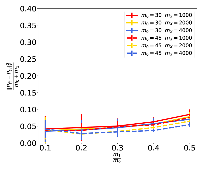
(a) Sigmoid activation function

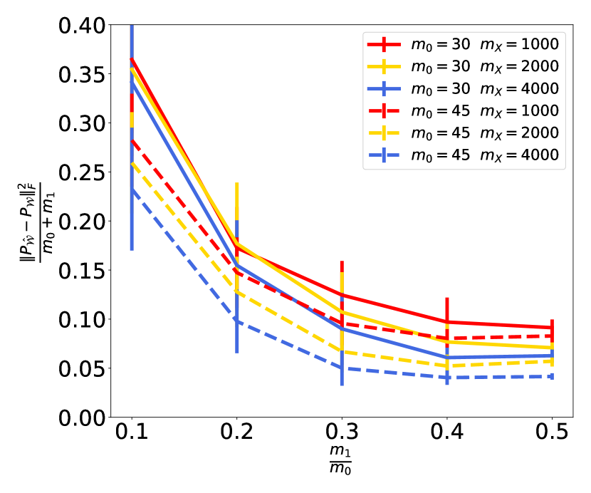
(b) $\tanh$ activation function

Figure 2: Error in approximating ${\cal W}$ for perturbed orthogonal weights and different activation functions.

In this section we present numerical experiments about the recovery of network weights $\{a_{i}:i\in[m_{0}]\}$ and $\{v_{\ell}:\ell\in[m_{1}]\}$ from few point queries of the network. The recovery procedure leverages the theoretical insights that have been provided in previous sections. Without much loss of generality, we neglect the active subspace reduction and focus on the case $d=m_{0}$. We construct an approximation $P_{\hat{\cal W}}\approx P_{{\cal W}}$ using Algorithm 2. Then we randomly generate a number of matrices $\{M^{k}_{0}:k\in[K]\}\in\hat{\cal W}\cap\mathbb{S}$, and compute the sequences $M^{k}_{j+1}=F_{\gamma}(M_{j}^{k})$ as in Algorithm 3. For each limiting matrix $\{M_{\infty}^{k}:k\in[K]\}$, we compute the largest eigenvector $u_{1}(M_{\infty}^{k})$, and then cluster $\{u_{1}(M_{\infty}^{k}):k\in[K]\}$ into $m=m_{0}+m_{1}$ classes using kMeans++. After projecting the resulting cluster centers onto $\mathbb{S}^{d-1}$, we obtain vectors $\{\hat{w}_{j}:j\in[m_{0}+m_{1}]\}$ that are used as approximations to $\{a_{i}:i\in[m_{0}]\}$ and $\{v_{\ell}:\ell\in[m_{1}]\}$.

We perform experiments for different scenarios, where either the activation function, or the construction of the network weights varies. Guided by our theoretical results, we pay particular attention to how the network architecture, e.g., $m_{0}$ and $m_{1}$, influences the simulation results. The entire procedure is rather flexible and can be adjusted in different ways, e.g. changing the distribution $\mu_{X}$. To provide a fair account of the success, we fix hyperparameters of the approach throughout all experiments. Test scenarios, hyperparameters, and error measures are reported below in more detail. Afterwards, we present and discuss the results.

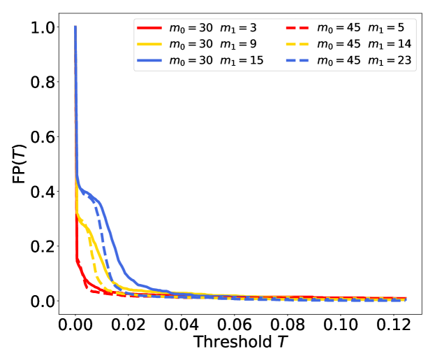
(a) False positives, sigmoid activation function

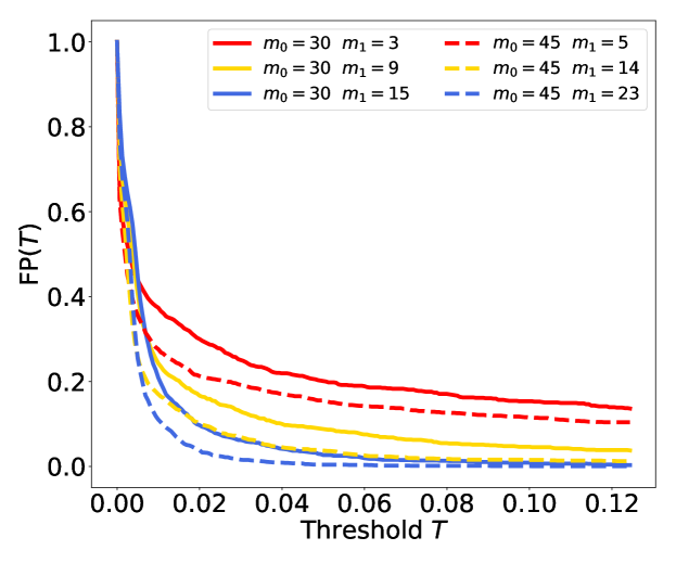
(b) False positives, $\tanh$ activation function

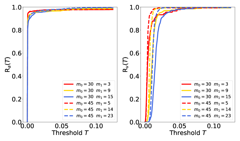
(c) Recovery rates, sigmoid activation function

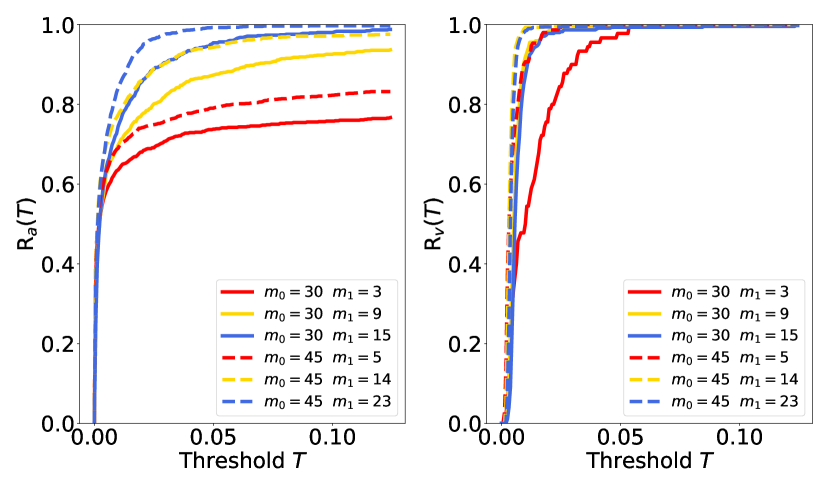
(d) Recovery rates, $\tanh$ activation function

Figure 3: False positive and recovery rates for perturbed orthogonal weights and for different activation functions.

Scenarios and construction of the networks

The network is constructed by choosing activation functions and network weights $\{a_{i}:i\in[m_{0}]\}$, $\{b_{\ell}:\ell\in[m_{1}]\}$, for which $v_{\ell}$ is then defined via $v_{\ell}=\frac{AG_{0}b_{\ell}}{\left\|{AG_{0}b_{\ell}}\right\|_{2}}$, see Definition 3. To construct activation functions, we set $g_{i}(t)=\phi(t+\theta_{i})$ for $i\in[m_{0}]$, and $h_{\ell}(t)=\phi(t+\tau_{\ell})$ for $\ell\in[m_{1}]$. We choose either $\phi(t)=\tanh(t)$, or $\phi(t)=\frac{1}{1+e^{-t}}-\frac{1}{2}$ (shifted sigmoid function), and sample offsets (called also biases) $\theta_{i}$, $\tau_{\ell}$ independently at random from ${\cal N}(0,0.01)$.

As made clear by our theory, see Theorem 13, a sufficient condition for successful recovery of the entangled weights is $\nu=C_{F}-1$ to be small, where $C_{F}$ is the upper frame constant of the entangled weights as in Definition 3. In the following numerical experiments we wish to verify how crucial is this requirement. Thus, we test two different scenarios for the weights. The first scenario, which is designed to best fulfill the sufficient condition $\nu\approx 0$, models both $\{a_{i}:i\in[m_{0}]\}$ and $\{b_{\ell}:\ell\in[m_{1}]\}$ as perturbed orthogonal systems. For their construction, we first sample orthogonal bases uniformly at random, and then apply a random perturbation. The perturbation is such that $(\sum_{i=1}^{m_{0}}(\sigma_{i}(A)-1)^{2})^{-1/2}\approx(\sum_{i=1}^{m_{1}}(\sigma_{i}(B)-1)^{2})^{-1/2}\approx 0.3$, where $\sigma_{i}(A)$ and $\sigma_{i}(B)$ denote singular values of $A$ and $B$. In the second case we sample the (entangled) weights independently from $\operatorname{Uni}({\mathbb{S}^{m_{0}-1}})$. In this situation, as the dimensionality $d=m_{0}$ is relatively small, the system will likely not fulfill well the condition $\nu\approx 0$; however, as the dimension $d=m_{0}$ is choosen larger, the weights tend to be more incoherent and gradually approaching the previous scenario.

Hyperparameters

Unless stated differently, we sample $m_{X}=1000$ Hessian locations from $\mu_{X}=\sqrt{m_{0}}\textrm{Uni}\left(\mathbb{S}^{m_{0}-1}\right)$, and use $\epsilon=10^{-5}$ in the finite difference approximation (25). We generate $1000$ random matrices $\{M_{0}^{k}:k\in[1000]\}$ by sampling $m^{k}\sim{\cal N}(0,\mathsf{Id}_{m_{0}+m_{1}})$, and by defining $M_{0}^{k}:=\mathbb{P}_{\mathbb{S}}(\sum_{i=1}^{m_{0}+m_{1}}m_{i}^{k}u_{i})$, where the $u_{i}$’s are as in Algorithm 2. The constant $\gamma=2$ is used in the definition of $F_{\gamma}$, and the iteration is stopped if $\lambda_{1}(M_{j+1}^{k})-\lambda_{1}(M_{j}^{k})<10^{-5}$, or after 200 iterations. kMeans++ is run with default settings using sklearn. All reported results are averages over 30 repetitions.

Error measures

Three error measures are reported:

• the normalized projection error $\frac{\|\hat{P}_{{\cal W}}-P_{{\cal W}}\|_{F}^{2}}{m_{0}+m_{1}}$,

• a false positive rate $\textrm{FP}(T)=\frac{\#\{j:E(\hat{w}_{j})>T\}}{m_{0}+m_{1}}$, where $T>0$ is a threshold, and $E(u)$ is defined by,

  $$E(u):=\min_{w\in\{\pm a_{i},\pm v_{\ell}:i\in[m_{0}],\ell\in[m_{1}]\}}\left\|{u-w}\right\|^{2}_{2},$$

• recovery rate $\textrm{R}_{a}(T)=\frac{\#\{i:{\cal E}(a_{i})<T\}}{m_{0}}$, and $\textrm{R}_{v}(T)=\frac{\#\{\ell:{\cal E}(v_{\ell})<T\}}{m_{1}}$, where

  $${\cal E}(u) :=\min_{w\in\{\pm\hat{w}_{j}:j\in[m_{0}+m_{1}]\}}\left\|{u-w}\right\|^{2}_{2}.$$

Results for perturbed orthogonal weights

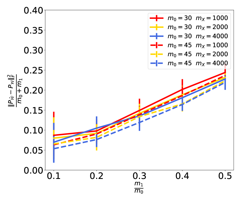
(a) Sigmoid activation function

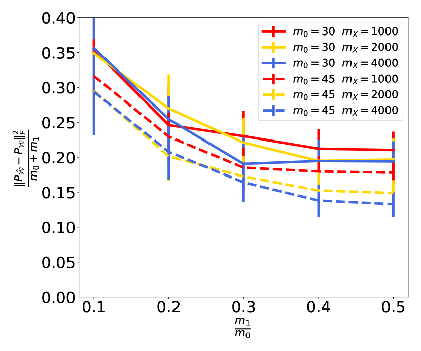
(b) $\tanh$ activation function

Figure 4: Error in approximating ${\cal W}$ for weights sampled independently from the unit sphere, and for different activation functions.

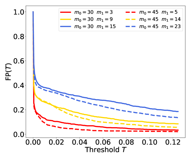
(a) False positives, sigmoid activation function

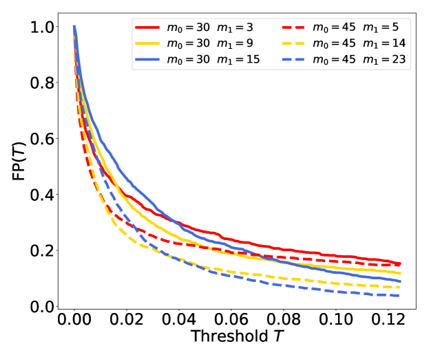
(b) False positives, $\tanh$ activation function

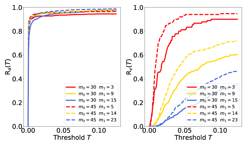
(c) Recovery rates, sigmoid activation function

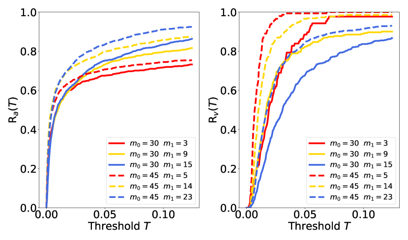
(d) Recovery rates, $\tanh$ activation function

Figure 5: False positive and recovery rates for weights sampled uniformly at random from the unit-sphere and for different activation functions.

The results of the study are presented in Figures 2 and 3, and show that our procedure typically recovers many of the network weights, while suffering only few false positives. Considering for example a sigmoidal network, we have almost perfect recovery of the weights in both layers at a threshold of $T=0.05$ for any network architecture, see Figures 3(a), 3(c). For a $\tanh$-network, the performance is slightly worse, but we still recover most weights in the second layer, and a large portion in the first layer at a reasonable threshold, see Figures 3(b), 3(d).

Inspecting the plots more closely, we can notice some shared trends and differences between sigmoid- and $\tanh$-networks. In both cases, the performance improves when increasing the input dimensionality or, equivalently, the number of neurons in the first layer, even though the number of weights that need to be recovered increases accordingly. This is particularly the case for $\tanh$-networks as visualized in Figures 3(b) and 3(d), and is most likely caused by reduced correlation of the weights in higher dimensions. As previously mentioned, the correlation is encoded within the constant $\nu=C_{F}-1$ used in the analysis in Section 3.

For fixed $m_{0}$ on the other hand, different activation functions react differently to changes of $m_{1}$. For $m_{1}$ larger, considering a sigmoid network, the projection error increases, and the recovery of weights in the second layer worsens as shown in Figures 2(a) and 3(c). This is expected by Theorem 4. Inspecting the results for $\tanh$-networks, the projection error actually decreases when increasing $m_{1}$, see Figure 2(b), and the recovery performance gets better. Figure 3(d) shows that especially weights in the first layer are more easily recovered if $m_{1}$ is large, such that the case $m_{0}=45$, $m_{1}=23$ allows for perfect recovery at a threshold $T=0.05$. This behavior can not be fully explained by our general theory, e.g. Theorem 4.

Results for random weights from the unit-sphere.

When sampling the weights independently from the unit-sphere, the recovery problem seems more challenging for moderate dimension $d=m_{0}$ and for both activation functions. This confirms the expectation that the smallness of $\nu=C_{F}-1$ is somehow crucial. Figures 5(c) and 5(d) suggest that especially recovering the weights of the second layer is more difficult than in the perturbed orthogonal case. Still, we achieve good performance in many cases. For sigmoid networks, Figure 5(c) shows that we always recover most weights in the first layer, and a large portion of weights in the second layer if $m_{1}/m_{0}$ is small. Moreover, keeping $m_{1}/m_{0}$ constant while increasing $m_{0}$ improves the performance significantly, as we expect from an improved constant $\nu=C_{F}-1$. Figures 5(a), 5(c) show almost perfect recovery for $m_{0}=45,\ m_{1}=5$, while suffering only few false positives.

For $\tanh$-networks, Figure 5(d) shows that increasing $m_{0}$ benefits recovery of weights in both layers, while increasing $m_{1}$ benefits recovery of first layer weights and harms recovery of second layer weights. We still achieve small false positive rates in Figure 5(b), and good recovery for $m_{0}=45$, and the trend continues when further increasing $m_{0}$.

Finally, a notable difference between the perturbed orthogonal case and the unit-sphere case is the behavior of the projection error $\|P_{\hat{\cal W}}-P_{{\cal W}}\|_{F}/(m_{0}+m_{1})$ for networks with sigmoid activation function. Comparing Figures 2(a) and 4(a), the dependency of the projection error on $m_{1}$ is stronger when sampling independently from the unit-sphere. This is explained by Theorem 4 since $\left\|{B}\right\|^{2}$ is independent of $m_{1}$ in the perturbed orthogonal case, and grows like $\mathcal{O}(\sqrt{m_{1}})$ when sampling from the unit-sphere.

5 Open problems

With the previous theoretical results of Section 3 and the numerical experiments of Section 4 we show how to reliably recover the entangled weights $\{\hat{w}_{j}:j\in[m_{0}+m_{1}]\}\approx\{w_{j}:j\in[m_{0}+m_{1}]\}=\{a_{i}:i\in[m_{0}]\}\cup\{v_{\ell}:\ell\in[m_{1}]\}$. However, some issues remain open.
(i) In Theorem 4 the dependency of $\alpha>0$ on the network architecture and on the input distribution $\mu_{X}$ is left implicit. However, it plays a crucial role for fully estimating the overall sample complexity.
(ii) While we could prove that Algorithm 3 is increasing the spectral norm of its iterates in $\hat{\cal W}\cap\mathbb{S}$, we could not show yet that it converges always to nearly rank-$1$ matrices in $\hat{\cal W}$, despite it is so numerically observed, see also Remark 3. We also could not exclude the existence of spurious local minimizers of the nonlinear program (46), as stated in Theorem 13. However, we conjecture that there are none or that they are somehow hard to observe numerically.
(iii) Obtaining the approximating vectors $\{\hat{w}_{j}:j\in[m_{0}+m_{1}]\}\approx\{w_{j}:j\in[m_{0}+m_{1}]\}=\{a_{i}:i\in[m_{0}]\}\cup\{v_{\ell}:\ell\in[m_{1}]\}$ does not suffice to reconstruct the entire network. In fact, it is impossible a priori to know whether $\hat{w}_{j}$ approximates one $a_{i}$ or some other $v_{\ell}$, up to sign and permutations, and the attribution to the corresponding layer needs to be derived from quering the network.
(iv) Once we obtained, up to sign and permutations, $\{\hat{a}_{i}:i\in[m_{0}]\}\approx\{a_{i}:i\in[m_{0}]\}$ and $\{\hat{v}_{\ell}:\ell\in[m_{1}]\}\approx\{v_{\ell}:\ell\in[m_{1}]\}$ from properly grouping $\{\hat{w}_{j}:j\in[m_{0}+m_{1}]\}$, it would remain to approximate/identify the activations functions $g_{i}$ and $h_{\ell}$. In the case where $g_{i}(\cdot)=\phi(\cdot-\theta_{i})$ and $h_{\ell}(\cdot)=\phi(\cdot-\tau_{\ell})$, this would simply mean to be able to identify the shifts $\theta_{i}$, $i\in[m_{0}]$, and $\tau_{\ell}$, $\ell\in[m_{1}]$. Such identification is also crucial for computing the matrix $G_{0}=\operatorname{diag}(g_{i}^{\prime}(0),\dots,g_{m_{0}}^{\prime}(0))$ which allows the disentanglement of the weights $b_{\ell}$ from the weights $A$ and $v_{\ell}=AG_{0}b_{\ell}/\|AG_{0}b_{\ell}\|_{2}$. At this point the network is fully reconstructed.
(v) The generalization of our approach to networks with more than two hidden layers is clearly the next relevant issue to be considered as a natural development of this work.

While problems (i) and (ii) seem to be difficult to solve by the methods we used in this paper, we think that problems (iii) and (iv) are solvable both theoretically and numerically with just a bit more effort. For a self-contained conclusion of this paper, in the following sections we sketch some possible approaches to these issues, as a glimpse towards future developments, which will be more exhaustively included in [22]. The generalization of our approach to networks with more than two hidden layers as mentioned in (v) is suprisingly simpler than one may expect, and it is in the course of finalization [22]. For a network $f(x):=f(x;W_{1},\dots,W_{L})=1^{T}g_{L}(W_{L}^{T}g_{L-1}(W_{L-1}^{T}\dots(g_{1}(W_{1}^{T}x))\dots)$, with $L>2$, again by second order differentiation is possible to obtain an approximation space

$$\hat{\cal W}\approx\operatorname{span}\{w_{1,i}\otimes w_{1,i},(W_{2}G_{1}w_{1,j})\otimes(W_{2}G_{1}w_{1,j}),\dots,(W_{L}G_{L}\dots W_{2}G_{1}w_{1,j})\otimes(W_{L}G_{L}\dots W_{2}G_{1}w_{1,j})\},$$

of the matrix space spanned by the tensors of entangled weights, where $G_{i}$ are suitable diagonal matrices depending on the activation functions. The tensors $(W_{k}G_{k}\dots W_{2}G_{1}w_{1,j})\otimes(W_{k}^{T}G_{k}\dots W_{2}^{T}G_{1}w_{1,j})$ can be again identified by a minimal rank principle. The disentanglement goes again by a layer by layer procedure as in this paper, see also [6].

6 Reconstruction of the entire network

In this section we address problems (iii) and (iv) as described in Section 5. Our final goal is of course to construct a two-layer network $\hat{f}$ with number of nodes equaling $m_{0}$ and $m_{1}$ such that $\hat{f}\approx f$. Additionally we also study whether the individual building blocks (e.g. matrices $\hat{A}$, $\hat{B}$, and biases in both layers) of $\hat{f}$ match their corresponding counterparts of $f$.

To construct $\hat{f}$, we first discuss how recovered entangled weights $\{\hat{w}_{i}:i\in[m_{0}+m_{1}]\}$ (see Section 4) can be assigned to either the first, or the second layer, depending on whether $\hat{w}_{j}$ approximates one of the $a_{i}$’s, or one of the $v_{\ell}$’s. Afterwards we discuss a modified gradient descent approach that optimizes the deparametrized network (its entangled weights are known at this point!) over the remaining, unknown parameters of the network function, e.g., biases $\theta_{i}$ and $\tau_{\ell}$.

6.1 Distinguishing first and second layer weights

Attributing approximate entangled weights to first or second layer is generally a challenging task. In fact, even the true weights $\{a_{i}:i\in[m_{0}]\}$, $\{v_{\ell}:\ell\in[m_{1}]\}$ can not be assigned to the correct layer based exclusively on their entries when no additional a priori information (e.g., some distributional assumptions) is available. Therefore, assigning $\hat{w}_{j}$, $j\in[m_{0}+m_{1}]$ to the correct layer requires using again the network $f$ itself, and thus to query additional information.

The strategy we sketch here is designed for sigmoidal activation functions and networks with (perturbed) orthogonal weights in each layer. Sigmoidal functions are monotonic, have bell-shaped first derivative, and are bounded by two horizontal asymptotes as the input tends to $\pm\infty$. If activation functions $\{g_{i}:i\in[m_{0}]\}$ and $\{h_{\ell}:\ell\in[m_{1}]\}$ are translated sigmoidal, their properties imply

$$\left\|{\nabla f(tw)}\right\|_{2}=\left(\sum_{i=1}^{m_{0}}g_{i}^{\prime}(ta_{i}^{T}w)^{2}\left(\sum^{m_{1}}_{\ell=1}h_{\ell}^{\prime}(b_{\ell}^{T}g(tA^{T}w))b_{i\ell}\right)^{2}\right)^{\frac{1}{2}}\rightarrow 0,\quad\textrm{as }t\rightarrow\infty,$$ (64)

whenever any direction $w$ has nonzero correlation $a_{i}^{T}w\neq 0$ with each first layer neuron in $\{a_{i}:i\in[m_{0}]\}$.

Assume now that $\{a_{i}:i\in[m_{0}]\}$ is a perturbed orthonormal system, and that second layer weights $\{b_{\ell}:\ell\in[m_{1}]\}$ are generic and dense (nonsparse). Recalling the definition $v_{\ell}=AG_{0}b_{\ell}/\left\|{AG_{0}b_{\ell}}\right\|$, the vector $v_{\ell}$ has, in this case, generally nonzero angle with each vector in $\{a_{i}:i\in[m_{0}]\}$, while $a_{i}^{\top}a_{j}\approx 0$ for any $i\neq j$. Utilizing this with observation (64), it follows that $\left\|{\nabla f(ta_{i})}\right\|$ is expected to tend to $0$ much slower than $\left\|{\nabla f(tv_{\ell}}\right\|$ as $t\rightarrow\infty$. In fact, if $\{a_{i}:i\in[m_{0}]\}$ was an exactly orthonormal system, $\left\|{\nabla f(ta_{i})}\right\|$ eventually would equal a positive constant when $t\rightarrow\infty$. We illustrate in Figure 6 the different behavior of the trajectories $t\to\left\|{\nabla f(tw)}\right\|_{2}$ for $w\in\{\hat{w}_{j}\approx a_{i}\mbox{ for some }i\}$ and for $w\in\{\hat{w}_{j}\approx v_{\ell}\mbox{ for some }\ell\}$.

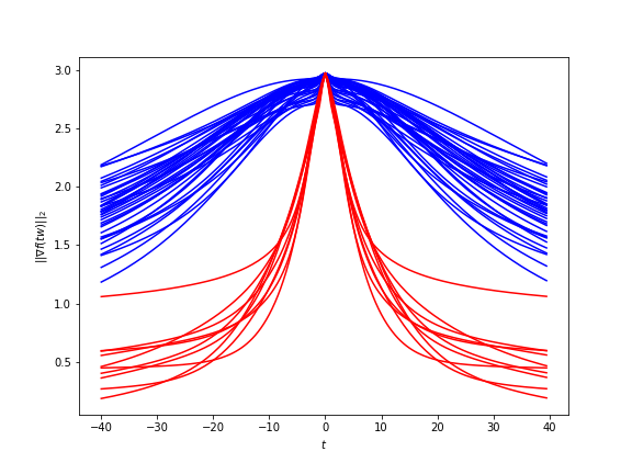
Figure 6: We illustrate the trajectories $t\to\left\|{\nabla f(tw)}\right\|_{2}$ for $w\in\{\hat{w}_{j}:j\in[m]\}$. The blue trajectories are those for $w\in\{\hat{w}_{j}\approx a_{i}\mbox{ for some }i\}$ and the red trajectories are those for $w\in\{\hat{w}_{j}\approx v_{\ell}\mbox{ for some }\ell\}$. We can observe the separation of the trajectories due to the different decay properties.

Practically, for $T\in\mathbb{N}$ and for each candidate vector in $\{\hat{w}_{j}:j\in[m_{0}+m_{1}]\}$ we query $f$ to compute $\Delta_{\epsilon}f(t_{k}\hat{w}_{j})$ for few steps $\{t_{k}:k\in[T]\}$ in order to approximate

$$\left\|{\left\|{\nabla f(t\hat{w}_{j})}\right\|_{2}}\right\|_{L_{2}([-\infty,\infty])}^{2}\approx\sum_{k=1}^{T}\left\|{\nabla f(t_{k}\hat{w}_{j})}\right\|^{2}\approx\sum_{k=1}^{T}\left\|{\Delta_{\epsilon}f(t_{k}\hat{w}_{j})}\right\|^{2}:=\hat{\cal I}(w_{j}).$$

Then we compute a permutation $\pi:[m]\rightarrow[m]$ to order the weights so that $\hat{\cal I}(w_{\pi(i)})\geq\hat{\cal I}(w_{\pi(j)})$ whenever $\pi(i)>\pi(j)$. The candidates $\{w_{\pi(j)}:j=1,\ldots,m_{0}\}$ have the slowest decay, respectively largest norms, and are thus assigned to the first layer. The remaining candidates $\{w_{\pi(\ell)}:\ell=m_{0}+1,\ldots,m_{1}\}$ are assigned to the second layer.

	$m_{0}=30$			$m_{0}=45$
Scenario	$m_{1}=3$	$m_{1}=9$	$m_{1}=15$	$m_{1}=5$	$m_{1}=14$	$m_{1}=23$
	${\cal L}_{1}$,   ${\cal L}_{2}$	${\cal L}_{1}$,   ${\cal L}_{2}$	${\cal L}_{1}$,   ${\cal L}_{2}$	${\cal L}_{1}$,   ${\cal L}_{2}$	${\cal L}_{1}$,   ${\cal L}_{2}$	${\cal L}_{1}$,   ${\cal L}_{2}$
POD/sig	$0.99$, $0.99$	$0.99$, $1.0$	$0.99$, $1.00$	$0.99$, $0.99$	$0.99$, $1.0$	$1.00$, $1.00$
POD/$\tanh$	$0.87$, $0.89$	$0.97$, $0.98$	$0.99$, $1.00$	$0.91$, $0.97$	$0.99$, $1.0$	$1.00$, $1.00$
$\mathbb{S}^{m_{0}-1}$/sig	$0.94$, $0.71$	$0.89$, $0.61$	$0.85$, $0.58$	$0.95$, $0.72$	$0.89$, $0.63$	$0.86$, $0.65$
$\mathbb{S}^{m_{0}-1}$/$\tanh$	$0.80$, $0.48$	$0.80$ $0.54$	$0.77$, $0.58$	$0.83$, $0.56$	$0.82$ $0.57$	$0.79$, $0.64$

Table 1: Success rates ${\cal L}_{1}$ and ${\cal L}_{2}$ (see (65)) when assigning candidates $\{\hat{w}_{i}:i\in[m_{0}+m_{1}]\}$ to either first or second layer of the network. We consider the same scenarios as in Section 4, e.g. POD/sig stands for perturbed orthogonal design with sigmoid activation, and $\mathbb{S}^{m_{0}-1}$/$\tanh$ for weights sampled independently from the unitsphere with $\tanh$ activation.

Numerical experiments

We have applied the proposed strategy to assign vectors $\{\hat{w}_{j}:j\in[m_{0}+m_{1}]\}$, which are outputs of experiments conducted in the Section 4, to either the first or the second layer. Since each $\hat{w}_{j}$ does not exactly correspond to a vector in $\{a_{i}:i\in[m_{0}]\}$ or $\{v_{\ell}:\ell\in[m_{1}]\}$, we assign a ground truth label $L_{j}=1$ to $\hat{w}_{j}$ if the closest vector to $\hat{w}_{j}$ belongs to $\{a_{i}:i\in[m_{0}]\}$, and $L_{j}=2$ if it belongs to the set $\{v_{\ell}:\ell\in[m_{1}]\}$. Denoting similarly the predicted label $\hat{L}_{j}=1$ if $\pi(j)\in\{1,\ldots,m_{0}\}$ and $\hat{L}_{j}=2$ otherwise, we compute the success rates

$${\cal L}_{1}:=\frac{\#\{j:L_{j}=1\textrm{ and }\hat{L}_{j}=1\}}{m_{0}},\quad{\cal L}_{2}:=\frac{\#\{j:L_{j}=2\textrm{ and }\hat{L}_{j}=2\}}{m_{1}}$$ (65)

to assess the proposed strategy. Hyperparameters are $\epsilon=10^{-5}$ for the step length in the finite difference approximation $\Delta_{\epsilon}f(\cdot)$, and $t_{k}=-20+k$ for $k\in[40]$.

The results for all four scenarios considered in Section 4 are reported in Table 1. We see that our simple strategy achieves remarkable success rates, in particular if the network weights in each layer represent perturbed orthogonal systems. If the weights are sampled uniformly from the unit sphere with moderated dimension $d=m_{0}$, then, as one may expect, the success rate drops. In fact, for small $d=m_{0}$, the vectors $\{a_{i}:i\in[m_{0}]\}$ tend to be less orthogonal, and thus the assumption $a_{i}^{\top}a_{j}\approx 0$ for $i\neq j$ is not satisfied anymore.

Finally, we stress that the proposed strategy is simple, efficient and relies only on few additional point queries of $f$ that are negligible compared to the recovery step itself (for reasonable query size $T$). In fact, the method relies on a single (nonlinear) feature of the map $t\mapsto\left\|{\nabla f(t\hat{w}_{j})}\right\|_{2}$ in order to decide upon the label of $\hat{w}_{j}$. We identify it as an interesting future investigation to develop more robust approaches, potentially using higher dimensional features of trajectories $t\to\left\|{\nabla f(t\hat{w}_{j})}\right\|_{2}$, to achieve high success rates even if $a_{i}^{\top}a_{j}\approx 0$ for $i\neq j$ may not hold anymore.

6.2 Reconstructing the network function using gradient descent

The previous section allows assigning unlabeled candidates $\{\hat{w}_{j}:j\in[m_{0}+m_{1}]\}$ to either the first or second layer, resulting in matrices $\hat{A}=[\hat{a}_{1}|\ldots|\hat{a}_{m_{0}}]$ and $\hat{V}=[\hat{v}_{1}|\ldots|\hat{v}_{m_{1}}]$ that ideally approximate $A$ and $V$ up to column signs and permutations. Assuming that the network $f\in{\cal F}(m_{0},m_{0},m_{1})$ is generated by shifts of one activation function, i.e., $g_{i}(t)=\phi(t+\theta_{i})$ and $h_{\ell}(t)=\phi(t+\tau_{\ell})$ for some $\phi$, this means only signs, permutations, and bias vectors $\theta\in\mathbb{R}^{m_{0}}$, $\tau\in\mathbb{R}^{m_{1}}$ are missing to fully reconstruct $f$. In this section we show how to identify these remaining parameters by applying a gradient descent method to minimize the least squares of the output misfit of the deparametrized network. In fact, as we clarify below, the original network $f$ can be explicitly described as a function of the known entangled weights $a_{i}$ and $v_{\ell}$ and of the unknown remaining parameters (signs, permutations, and biases), see Proposition 22 and Corollary 2 below.

Let now ${\cal D}_{m}$ denote the set of $m\times m$ diagonal matrices, and define a parameter space $\Omega:={\cal D}_{m_{1}}\times{\cal D}_{m_{0}}\times{\cal D}_{m_{0}}\times\mathbb{R}^{m_{0}}\times\mathbb{R}^{m_{1}}$. To reconstruct the original network $f$, we propose to fit parameters $(D_{1},D_{2},D_{3},w,z)\in\Omega$ of a function $\hat{f}:\mathbb{R}^{m_{0}}\times\Omega\rightarrow\mathbb{R}$ defined by

$$\hat{f}(x;D_{1},D_{2},D_{3},w,z) =1^{\top}\phi(D_{1}\hat{V}^{\top}\hat{A}^{-\top}D_{2}\phi(D_{3}\hat{A}^{\top}x+w)+z)$$

to a number of additionally sampled points $\{(X_{i},Y_{i}):i\in[m_{f}]\}$ where $Y_{i}=f(X_{i})$ and $X_{i}\sim{\cal N}(0,\mathsf{Id}_{m_{0}})$. The parameter fitting can be formulated as solving the least squares

$$\min_{(D_{1},D_{2},D_{3},w,z)\in\Omega}J(D_{1},D_{2},D_{3},w,z):=\sum_{i=1}^{m_{f}}\left(Y_{i}-\hat{f}(X_{i};D_{1},D_{2},D_{3},w,z)\right)^{2}.$$ (66)

We note that, due to the identification of the entangled weights and deparametrization of the problem, $\dim(\Omega)=3m_{0}+2m_{1}$, which implies that the least squares has significantly fewer free parameters compared to the number $m_{0}^{2}+(m_{0}\times m_{1})+(m_{0}+m_{1})$ of original parameters of the entire network. Hence, our previous theoretical results of Section 3 and numerical experiments of Section 4 greatly scale down the usual effort of fitting all parameters at once. We may also mention at this point that the optimization (66) might have multiple global solutions due to possible symmetries, see also [19] and Remark 4, and we shall try to keep into account the most obvious ones in our numerical experiments below.
We will now show that there exists parameters $(D_{1},D_{2},D_{3},w,z)\in\Omega$ that allow for exact recovery of the original network, whenever $\hat{A}$ and $\hat{V}$ are correct up to signs and permutation. We first need the following proposition that provides a different reparametrization of the network using $\hat{A}$ and $\hat{V}$. The proof of the proposition requires only elementary linear algebra, and properties of sign and permutation matrices. Details are deferred to Appendix A.3.

Proposition 22.

Let $f\in{\cal F}(m_{0},m_{0},m_{1})$ with $g_{i}(t)=\phi(t+\theta_{i})$ and $h_{\ell}(t)=\phi(t+\tau_{\ell})$, and define the function $\tilde{f}:\mathbb{R}^{m_{0}}\times{\cal D}_{m_{0}}\times{\cal D}_{m_{1}}\times\mathbb{R}^{m_{0}}\times\mathbb{R}^{m_{1}}\rightarrow\mathbb{R}$ via

$$\tilde{f}(x;D,D^{\prime},w,z) =1^{\top}\phi(D^{\prime}\hat{B}^{\top}\phi(D\hat{A}^{\top}x+w)+z),\quad\textrm{with}\quad\hat{b}_{l}:=\frac{\operatorname{diag}\left(\left(\phi^{\prime}(w)\right)^{-1}\right)D\hat{A}^{-1}\hat{v}_{\ell}}{\left\|{\operatorname{diag}\left(\left(\phi^{\prime}(w)\right)^{-1}\right)D\hat{A}^{-1}\hat{v}_{\ell}}\right\|}.$$

If there are sign matrices $S_{A}$, $S_{V}$, and permutations $\pi_{A}$, $\pi_{V}$ such that $A\pi_{A}=\hat{A}S_{A}$, $V\pi_{V}=\hat{V}S_{V}$, then we have $f(x)=\tilde{f}(x;S_{A},S_{V},\pi_{A}^{\top}\theta,\pi_{V}^{\top}\tau)$.

We note here that replacing $\hat{f}$ by $\tilde{f}$ in (66) is tempting because it further reduces the number of parameters ($\dim({\cal D}_{m_{0}}\times{\cal D}_{m_{1}}\times\mathbb{R}^{m_{0}}\times\mathbb{R}^{m_{1}})=2(m_{0}+m_{1})$), but, by an explicit computation, one can show that evaluating the gradient of $\tilde{f}$ with respect to $D$ requires also the evaluation of $D^{-1}$. Having in mind that $D$ ideally converges to $S_{A}$ during the optimization, diagonal entries of $D$ are likely to cross zero while optimizing. Thus such minimization may result unstable, and we instead work with $\hat{f}$. The following Corollary shows that also this form allows finding optimal parameters leading to the original network.

Corollary 2.

Let $f\in{\cal F}(m_{0},m_{0},m_{1})$ with $g_{i}(t)=\phi(t+\theta_{i})$ and $h_{\ell}(t)=\phi(t+\tau_{\ell})$. If there exist sign matrices $S_{A}$, $S_{V}$, and permutations $\pi_{A}$, $\pi_{V}$ such that $A\pi_{A}=\hat{A}S_{A}$, $V\pi_{V}=\hat{V}S_{V}$, there exist diagonal matrices $D_{1},D_{2}$ such that $f(x)=\hat{f}(x;D_{1},D_{2},S_{A},\pi_{A}^{\top}\theta,\pi_{V}^{\top}\tau)$.

Proof.

Based on Proposition 22 we can rewrite $f(x)=1^{\top}\phi(S_{V}\hat{B}^{\top}\phi(S_{A}\hat{A}^{\top}x+\pi_{A}^{\top}w)+\pi_{V}^{\top}z)$, so it remains to show that $S_{V}\hat{B}^{\top}=D_{1}\hat{V}^{\top}\hat{A}^{-\top}D_{2}$ for diagonal matrices $D_{1}$, $D_{2}$. First we note

$$\operatorname{diag}(\phi^{\prime}(\pi_{A}^{\top}\theta)^{-1})=\pi_{A}^{\top}\operatorname{diag}(\phi^{\prime}(\theta)^{-1})\pi_{A}=\pi_{A}^{\top}G^{-1}\pi_{A}.$$

Using this, and $D=S_{A}$ in the definition of $\hat{B}$ in Proposition 22, it follows that

$$\hat{B}^{\top}=\operatorname{diag}(\|\pi_{A}^{\top}G^{-1}\pi_{A}S_{A}\hat{A}^{-1}v_{1}\|,\ldots,\|\pi_{A}^{\top}G^{-1}\pi_{A}S_{A}\hat{A}^{-1}v_{m_{1}}\|)\hat{V}^{\top}\hat{A}^{-\top}S_{A}\pi_{A}^{\top}G^{-1}\pi_{A}$$

Multiplying by $S_{V}$ from the left, we obtain

$$S_{V}\hat{B}^{\top}=\underbrace{S_{V}\operatorname{diag}(\|\pi_{A}^{\top}G^{-1}\pi_{A}S_{A}\hat{A}^{-1}v_{1}\|,\ldots,\|\pi_{A}^{\top}G^{-1}\pi_{A}S_{A}\hat{A}^{-1}v_{m_{1}}\|)}_{=D_{1}}\hat{V}^{\top}\hat{A}^{-\top}\underbrace{S_{A}\pi_{A}^{\top}G^{-1}\pi_{A}}_{=D_{2}}.$$

∎

Remark 4 (Simplification for odd functions).

If $\phi$ in Proposition 22 satisfies $\phi(-t)=-\phi(t)$, then $\hat{f}(x;D_{1},SD_{2},SD_{3},Sw,z)=\hat{f}(x;D_{1},D_{2},D_{3},w,z)$ for arbitrary sign matrix $S\in{\cal D}_{m_{0}}$. Thus, choosing $S=S_{A}$, there are also diagonal $D_{1}$ and $D_{2}$ with $f(x)=\hat{f}(x;D_{1},D_{2},\mathsf{Id}_{m_{0}},S_{A}\pi_{A}^{\top}w,\pi_{V}^{\top}\tau)$.

Assuming $\hat{A}$ and $\hat{V}$ are correct up to sign and permutation, Corollary 2 implies that $J=0$ is the global optimum, and it is attained by parameters leading to the original network $f$. Furthermore Remark 4 implies that there is ambiguity with respect to $D_{3}$, if $\phi$ is an odd function. Thus we can also prescribe $D_{3}=\mathsf{Id}_{m_{0}}$ and neglect optimizing this variable if $\phi$ is odd.

We now study numerically the feasibility of (66). First, we consider the case $\hat{A}=A$ and $\hat{V}=V$ to assess (66), isolated so not to suffer possible errors from other parts of our learning procedure (see Section 4 and Section 6.1). Afterwards we take into consideration also these additional approximations, and present results for $\hat{A}\approx A$ and $\hat{V}\approx V$.

Numerical experiments

		$m_{0}=30$			$m_{0}=45$
Scenario		$m_{1}=3$	$m_{1}=9$	$m_{1}=15$	$m_{1}=5$	$m_{1}=14$	$m_{1}=23$
POD/sig	MSE	$1.2e^{-5}$	$5.4e^{-6}$	$4.7e^{-5}$	$1.1e^{-5}$	$4.6e^{-6}$	$5.6e^{-6}$
	$E_{\infty}$	$4.3e^{-3}$	$3.8e^{-3}$	$4.9e^{-3}$	$3.9e^{-3}$	$3.4e^{-3}$	$4.4e^{-3}$
	$E_{\theta}$	$4.1e^{-1}$	$2.7e^{-1}$	$1.7e^{-1}$	$4.4e^{-1}$	$2.6e^{-1}$	$1.7e{-1}$
	$E_{\tau}$	$3.9e^{-2}$	$1.9e^{-2}$	$3.1e^{-2}$	$4.4e^{-2}$	$2.1e^{-2}$	$3.3e^{-2}$
POD/$\tanh$	MSE	$1.9e^{-7}$	$1.5e^{-9}$	$1.2e^{-10}$	$1.1e^{-7}$	$7.5e^{-10}$	$8.4e^{-12}$
	$E_{\infty}$	$7.3e^{-4}$	$5.4e^{-5}$	$1.3e^{-5}$	$4.6e^{-4}$	$4.2e^{-5}$	$3.6e^{-6}$
	$E_{\theta}$	$2.9e^{-3}$	$6.8e^{-8}$	$4.2e^{-8}$	$2.6e^{-3}$	$2.1e^{-7}$	$1.5e^{-9}$
	$E_{\tau}$	$3.3e^{-4}$	$1.1e^{-7}$	$2.1e^{-8}$	$1.1e^{-4}$	$8.4e^{-8}$	$9.5e^{-10}$
$\mathbb{S}^{m_{0}-1}$/sig	MSE	$1.3e^{-5}$	$9.7e^{-6}$	$1.4e^{-5}$	$1.2e^{-5}$	$9.4e^{-6}$	$1.6e^{-5}$
	$E_{\infty}$	$4.9e^{-3}$	$5.7e^{-3}$	$8.2e^{-3}$	$4.5e^{-3}$	$5.5e^{-3}$	$8.5e^{-3}$
	$E_{\theta}$	$4.5e^{-1}$	$3.5e^{-1}$	$3.0e^{-1}$	$4.5e^{-1}$	$2.7e^{-1}$	$2.4e^{-1}$
	$E_{\tau}$	$3.7e^{-2}$	$7.0e^{-2}$	$1.2e^{-1}$	$5.3e^{-2}$	$5.5e^{-2}$	$1.1e^{-1}$
$\mathbb{S}^{m_{0}-1}$/$\tanh$	MSE	$4.4e^{-7}$	$4.8e^{-9}$	$4.9e^{-10}$	$7.7e^{-8}$	$1.5e^{-9}$	$1.6e^{-11}$
	$E_{\infty}$	$1.3e^{-3}$	$1.4e^{-4}$	$3.0e^{-5}$	$5.0e^{-4}$	$6.0e^{-5}$	$5.7e^{-6}$
	$E_{\theta}$	$1.9e^{-2}$	$1.5e^{-6}$	$3.1e^{-7}$	$3.7e^{-4}$	$3.5e^{-7}$	$4.9e^{-9}$
	$E_{\tau}$	$7.6e^{-4}$	$1.4e^{-6}$	$5.7e^{-8}$	$7.5e^{-5}$	$2.8e^{-7}$	$1.5e^{-9}$

Table 2: Errors of the reconstructed network using (66) when prescribing $\hat{A}=A$ and $\hat{V}=V$. The scenarios correspond to those in Section 4 and Section 6.1.

		$m_{0}=30$			$m_{0}=45$
Scenario		$m_{1}=3$	$m_{1}=9$	$m_{1}=15$	$m_{1}=5$	$m_{1}=14$	$m_{1}=23$
POD/sig	MSE	$6.4e^{-5}$	$3.1e^{-2}$	$2.9e^{-2}$	$6.8e^{-5}$	$1.1e^{-2}$	$5.4e^{-4}$
	$E_{\infty}$	$1.1e^{-2}$	$7.9e^{-2}$	$9.0e^{-2}$	$1.4e^{-2}$	$4.5e^{-2}$	$4.7e^{-2}$
	Trials [$\%$]	$63$	$80$	$90$	$37$	$67$	$93$
POD/$\tanh$	MSE	$-$	$2.7e^{-2}$	$8.9e^{-3}$	$-$	$4.2e^{-3}$	$7.7e^{-3}$
	$E_{\infty}$	$-$	$1.9e^{-1}$	$1.2e^{-1}$	$-$	$8.3e^{-2}$	$9.7e^{-2}$
	Trials [$\%$]	$0$	$23$	$76$	$0$	$43$	$96$

Table 3: Errors of the reconstructed network using (66) when using approximated $\hat{A}\approx A$ and $\hat{V}\approx V$ (up to sign and permutation). Trials indicates the percentage of repititions where $\hat{A}$ and $\hat{V}$ satisfy (67). The scenarios correspond to those in Section 4 and Section 6.1.

We minimize (66) by standard gradient descent and learning rate $0.5$ if $\phi(t)=\frac{1}{1+e^{-t}}-\frac{1}{2}$ (shifted sigmoid), respectively learning rate $0.025$ if $\phi(t)=\tanh(t)$. We sample $m_{f}=10(m_{0}+m_{1})$ additional points, which is only slightly more than the number of free parameters. Gradient descent is run for 500K iterations (due to small number of variables, this is not time consuming), and only prematurely stopped it, if the iteration stalls. Initially we set $D_{2}=D_{3}=\mathsf{Id}_{m_{0}}$, and all other variables are set to random draws from ${\cal N}(0,0.1)$.

Denoting $\omega^{*}=(D_{1}^{*},D_{2}^{*},D_{3}^{*},w^{*},z^{*})\in\Omega$ as the gradient descent output, we measure the relative mean squared error (MSE) and the relative $L_{\infty}$-error

$$\textrm{MSE}=\frac{\sum_{i=1}^{m_{\textrm{test}}}(\hat{f}(Z_{i};\omega^{*})-f(Z_{i}))^{2}}{\sum_{i=1}^{m_{\textrm{test}}}f(Z_{i})^{2}},\quad\textrm{E}_{\infty}=\frac{\max_{i\in[m_{\textrm{test}}]}\left|{\hat{f}(Z_{i};\omega^{*})-f(Z_{i})}\right|}{\max_{i\in[m_{\textrm{test}}]}\left|{f(Z_{i})}\right|},$$

using $m_{\textrm{test}}=50000$ samples $Z_{i}\sim{\cal N}(0,\mathsf{Id}_{m_{0}})$. Moreover, we also report the relative bias errors

$$E_{\theta}=\frac{\left\|{w^{*}-\theta}\right\|^{2}}{\left\|{\theta}\right\|^{2}},\quad E_{\eta}=\frac{\left\|{z^{*}-\eta}\right\|^{2}}{\left\|{\eta}\right\|^{2}},$$

which indicate if the original bias vectors are recovered. We repeat each experiments 30 times, and report averaged values.

Table 2 presents the results of the experiments and shows that we reconstruct a network function that is very close to the original network $f$ in both $L_{2}$ and $L_{\infty}$ norm, and in every scenario. The maximal error is $\approx 10^{-3}$, which is likely further reducible by increasing the number of gradient descent iterations, or using finer tuned learning rates or acceleration methods. Therefore, the experiments strongly suggest that we are indeed reconstructing a function that approximates $f$ uniformly well. Inspecting the errors $E_{\theta}$ and $E_{\eta}$ also supports this claim, at least in all scenarios where the $\tanh$ activation is used. In many cases the relative errors are below $10^{-7}$, implying that we recover the original bias vectors of the network. Suprisingly, the accuracy of recovered biases slightly drops of few orders of magnitude in the sigmoid case, despite convincing results when measuring predictive performance in $L_{2}$ and $E_{\infty}$. We believe that this is due to faster flattening of the gradients around the stationary point compared to the case of a $\tanh$ activation function, and that it can be improved by using more sophisticated strategies of choosing a gradient descent step size. We also tested (66) when fixing $D=\mathsf{Id}_{m_{0}}$ since $\tanh$ and the shifted sigmoid are odd functions, and thus Remark 4 applies. The results are consistently slightly better than Table 2, but are qualitatively similar.

We ran similar experiments for perturbed orthogonal weights and when using $\hat{A}$ and $\hat{V}$ precomputed with the methods we described in Section 4 and Section 6.1. The quality of the results varies dependent on whether $\hat{A}\approx A$ and $\hat{V}\approx V$ (up to sign and permutation) holds, or a fraction of the weights has not been recovered. To isolate cases where $\hat{A}\approx A$ and $\hat{V}\approx V$ holds, we compute averaged MSE and $L_{\infty}$ over all trials satisfying

$$\sum_{i=1}^{m_{0}}{\cal E}(a_{i})+\sum_{\ell=1}^{m_{1}}{\cal E}(v_{\ell})<0.5,\quad\textrm{(see Section \ref{sec:numerical_NNprofiles} for the Definition of }{\cal E}).$$ (67)

We report the averaged errors, and the number of trials satisfying this condition in Table 3. It shows that the reconstructed function is close to the original function, even if the weights are only approximately correct. Therefore we conclude that that minimizing (66) provides a very efficient way of learning the remaining network parameters from just few additional samples, once entangled network weights $A$ and $V$ are (approximately) known.

Appendix A Appendix

The following Lemma implies that $\{a_{1}\otimes a_{1},\ldots a_{m_{0}}\otimes a_{m_{0}},v_{1}\otimes v_{1},\ldots,v_{m_{1}}\otimes v_{m_{1}}\}$ satisfying the properties of Definition 3 is a system of linearly independent matrices.

Lemma 23.

Let $\{z_{1},\ldots,z_{m}\}\subset\mathbb{R}^{m}$ have unit norm and satisfy $\sum_{i=1}^{m}\left\langle z_{j},z_{i}\right\rangle^{2}\leq C_{F}$ for all $j=1,\ldots,m$. If $1<C_{F}<2$, the system $\{z_{1}\otimes z_{1},\ldots,z_{m}\otimes z_{m}\}$ is linearly independent.

Proof.

Assume to the contrary the $\{z_{1}\otimes z_{1},\ldots,z_{m}\otimes z_{m}\}$ are not linearly independent, then there exists $\sigma\neq 0\in\mathbb{R}^{m}$ with $0=\sum_{i=1}^{m}\sigma_{i}z_{i}\otimes z_{i}$, or equivalently $0=\sum_{i=1}^{m}\sigma_{i}\langle x,z_{i}\rangle^{2}$ for all $x\in\mathbb{R}^{d}$. Without loss of generality assume $\left\|{\sigma}\right\|_{\infty}=\max_{i}\sigma_{i}$ (otherwise we multiply the representation by $-1$), and denote by $i^{*}$ the index achieving the maximum. Then we have

$$0 =\sum\limits_{i=1}^{N}\sigma_{i}\left\langle z_{i},z_{i^{*}}\right\rangle^{2}=\sigma_{i^{*}}\left\|{z_{i^{*}}}\right\|^{2}+\sum\limits_{i\neq i^{*}}\sigma_{i}\left\langle z_{i},z_{i^{*}}\right\rangle^{2}\geq\sigma_{i^{*}}\left\|{z_{i^{*}}}\right\|^{2}+\min_{i}\sigma_{i}\sum\limits_{i\neq i^{*}}\left\langle z_{i},z_{i^{*}}\right\rangle^{2}$$

Since $\min_{i}\sigma_{i}\geq 0$ immediately yields a contradiction, we continue with the case $\min_{i}\sigma_{i}<0$. We can further bound

$$0 \geq\sigma_{i^{*}}\left\|{z_{i^{*}}}\right\|^{2}+\min_{i}\sigma_{i}\sum\limits_{i\neq i^{*}}\left\langle z_{i},z_{i^{*}}\right\rangle^{2}\geq\sigma_{i^{*}}+\min_{i}\sigma_{i}\left(C_{F}-1\right)\left\|{z_{i}^{*}}\right\|^{2}=\sigma_{i^{*}}+\min_{i}\sigma_{i}\left(C_{F}-1\right),$$

and by division through $\left(C_{F}-1\right)$, and subtracting $\min_{i}\sigma_{i}$ we obtain $\left|{\min_{i}\sigma_{i}}\right|\geq\sigma_{i^{*}}(C_{F}-1)^{-1}$. Since $(C_{F}-1)^{-1}>1$, this yields the contradiction $\left\|{\sigma}\right\|_{\infty}\geq\left|{\min_{i}\sigma_{i}}\right|>\sigma_{i^{*}}=\left\|{\sigma}\right\|_{\infty}$. ∎

The linear independence of the system $\{a_{1}\otimes a_{1},\ldots a_{m_{0}}\otimes a_{m_{0}},v_{1}\otimes v_{1},\ldots,v_{m_{1}}\otimes v_{m_{1}}\}$ implies that it is a Riesz basis for ${\cal W}:=\operatorname{span}{a_{1}\otimes a_{1},\ldots a_{m_{0}}\otimes a_{m_{0}},v_{1}\otimes v_{1},\ldots,v_{m_{1}}\otimes v_{m_{1}}}$. As such there exists constants $c_{r}$, $C_{R}$ such that for every $\sigma\in\mathbb{R}^{m_{0}+m_{1}}$

$$c_{r}\left\|{\sigma}\right\|_{2}^{2}\leq\left\|{\sum_{i=1}^{m_{0}}\sigma_{i}a_{i}\otimes a_{i}+\sum_{i=1}^{m_{1}}\sigma_{m_{0}+i}v_{i}\otimes v_{i}}\right\|^{2}\leq C_{R}\left\|{\sigma}\right\|_{2}^{2}.$$ (68)

A.1 Additional proofs for Section 2

Proof of Lemma 5.

Fix any pair $k,n\in[d]$ and define $\phi(t)=f(x+te_{k}+\epsilon e_{n})-f(x+te_{k})$, where $e_{k}$ denotes the $k$-th standard vector. By the mean value theorem and for $\Delta^{2}_{\epsilon}f(x)\in\mathbb{R}^{d\times d}$ given as in (25), there exist $0<\xi_{1},\xi_{2}<\epsilon$ such that

$$(\Delta^{2}_{\epsilon}[f](x))_{kn} =\frac{\phi(\epsilon)-\phi(0)}{\epsilon^{2}}=\frac{\phi^{\prime}(\xi_{1})}{\epsilon}$$

$$=\frac{\frac{\partial f}{\partial x_{k}}(x+\xi_{1}e_{k}+\epsilon e_{n})-\frac{\partial f}{\partial x_{k}}(x+\xi_{1}e_{k})}{\epsilon}$$

$$=\frac{\partial^{2}f}{\partial x_{k}\partial x_{n}}(x+\xi_{1}e_{k}+\xi_{2}e_{n}).$$

Hence, we obtain

$$\lvert\nabla^{2}f((x))_{kn}-(\Delta^{2}_{\epsilon}[f](x))_{kn}\rvert=\left|\frac{\partial^{2}f}{\partial x_{k}\partial x_{n}}(x)-\frac{\partial^{2}f}{\partial x_{k}\partial x_{n}}(x+\xi_{1}e_{k}+\xi_{2}e_{n})\right|.$$

Assume $k,n$ to be fixed and denote $\tilde{x}=x+\xi_{1}e_{k}+\xi_{2}e_{n}$. By recalling our definition of $\nabla^{2}f(x)$ in (17), it follows $\frac{\partial^{2}f}{\partial x_{k}\partial x_{n}}(x)=\varphi_{1}(x)+\varphi_{2}(x)$, where

$$\varphi_{1}(x) :=\sum^{m_{1}}_{\ell=1}\sum^{m_{0}}_{i,j=1}h_{\ell}^{\prime\prime}(b_{\ell}^{T}g(A^{T}x))g_{i}^{\prime}(a_{i}^{T}x)g_{j}^{\prime}(a_{j}^{T}x)a_{ki}a_{nj}b_{i\ell}b_{j\ell},$$

$$\varphi_{2}(x) :=\sum^{m_{1}}_{\ell=1}\sum^{m_{0}}_{i=1}h_{\ell}^{\prime}(b_{\ell}^{T}g(A^{T}x))g_{i}^{\prime\prime}(a_{i}^{T}x)a_{ki}a_{ni}b_{i\ell}.$$

Thus

$$\lvert(\nabla^{2}f(x))_{kn}-(\Delta^{2}_{\epsilon}[f](x))_{kn}\rvert\leq\lvert\varphi_{1}(x)-\varphi_{1}(\tilde{x})\rvert+\lvert\varphi_{2}(x)-\varphi_{2}(\tilde{x})\rvert.$$

As before, we start by applying the Lipschitz continuity to the summands of $\lvert\varphi_{1}(x)-\varphi_{1}(\tilde{x})\rvert$:

$$\lvert h_{\ell}^{\prime\prime}(b_{\ell}^{T}g(A^{T}x))g_{i}^{\prime}(a_{i}^{T}x)g_{j}^{\prime}(a_{j}^{T}x)-h_{\ell}^{\prime\prime}(b_{\ell}^{T}g(A^{T}\tilde{x}))g_{i}^{\prime}(a_{i}^{T}\tilde{x})g_{j}^{\prime}(a_{j}^{T}\tilde{x})\rvert$$

$$\leq \lvert h_{\ell}^{\prime\prime}(b_{\ell}^{T}g(A^{T}x))g_{i}^{\prime}(a_{i}^{T}x)g_{j}^{\prime}(a_{j}^{T}x)-h_{\ell}^{\prime\prime}(b_{\ell}^{T}g(A^{T}x))g_{i}^{\prime}(a_{i}^{T}\tilde{x})g_{j}^{\prime}(a_{j}^{T}\tilde{x})\rvert$$

$$+ \lvert h_{\ell}^{\prime\prime}(b_{\ell}^{T}g(A^{T}x))g_{i}^{\prime}(a_{i}^{T}\tilde{x})g_{j}^{\prime}(a_{j}^{T}\tilde{x})-h_{\ell}^{\prime\prime}(b_{\ell}^{T}g(A^{T}\tilde{x}))g_{i}^{\prime}(a_{i}^{T}\tilde{x})g_{j}^{\prime}(a_{j}^{T}\tilde{x})\rvert$$

$$\leq \eta_{2}\lvert g_{i}^{\prime}(a_{i}^{T}x)g_{j}^{\prime}(a_{j}^{T}x)-g_{i}^{\prime}(a_{i}^{T}\tilde{x})g_{j}^{\prime}(a_{j}^{T}\tilde{x})\rvert+\kappa_{1}^{2}\lvert h_{\ell}^{\prime\prime}(b_{\ell}^{T}g(A^{T}x))-h_{\ell}^{\prime\prime}(b_{\ell}^{T}g(A^{T}\tilde{x}))\rvert$$

$$\leq \eta_{2}\left[\lvert g_{i}^{\prime}(a_{i}^{T}x)g_{j}^{\prime}(a_{j}^{T}x)-g_{i}^{\prime}(a_{i}^{T}\tilde{x})g_{j}^{\prime}(a_{j}^{T}x)\rvert+\lvert g_{i}^{\prime}(a_{i}^{T}\tilde{x})g_{j}^{\prime}(a_{j}^{T}x)-g_{i}^{\prime}(a_{i}^{T}\tilde{x})g_{j}^{\prime}(a_{j}^{T}\tilde{x})\rvert\right]$$

$$+ \kappa_{1}^{2}\eta_{3}\left|\sum^{m_{0}}_{I=1}b_{I\ell}\left(g_{I}(a_{I}^{T}x)-g_{I}(a_{I}^{T}\tilde{x})\right)\right|$$

$$\leq \eta_{2}\left[\kappa_{1}\lvert g_{i}^{\prime}(a_{i}^{T}x)-g_{i}^{\prime}(a_{i}^{T}\tilde{x})\rvert+\kappa_{1}\lvert g_{j}^{\prime}(a_{j}^{T}x)-g_{j}^{\prime}(a_{j}^{T}\tilde{x})\rvert\right]+\kappa_{1}^{3}\eta_{3}\left|\sum^{m_{0}}_{I=1}b_{Il}a_{I}^{T}(x-\tilde{x})\right|$$

$$\leq \eta_{2}\kappa_{1}\kappa_{2}\left[\lvert a_{i}^{T}(x-\tilde{x})\rvert+\lvert a_{j}^{T}(x-\tilde{x})\rvert\right]+\kappa_{1}^{3}\eta_{3}\left|\sum^{m_{0}}_{I=1}b_{I\ell}a_{I}^{T}(x-\tilde{x})\right|$$

$$\leq \eta_{2}\kappa_{1}\kappa_{2}\left[\lvert\xi_{1}a_{ki}+\xi_{2}a_{ni}\rvert+\lvert\xi_{1}a_{kj}+\xi_{2}a_{nj}\rvert\right]+\kappa_{1}^{3}\eta_{3}\left|\sum^{m_{0}}_{I=1}b_{I\ell}(\xi_{1}a_{kI}+\xi_{2}a_{nI})\right|$$

$$\leq \eta_{2}\kappa_{1}\kappa_{2}\epsilon\left[\lvert a_{ki}\rvert+\lvert a_{ni}\rvert+\lvert a_{kj}\rvert+\lvert a_{nj}\rvert\right]+\kappa_{1}^{3}\eta_{3}\epsilon\sum^{m_{0}}_{I=1}\lvert b_{I\ell}\rvert(\lvert a_{kI}\rvert+\lvert a_{nI}\rvert)$$

$$\leq \tilde{C}\epsilon\left[\lvert a_{ki}\rvert+\lvert a_{ni}\rvert+\lvert a_{kj}\rvert+\lvert a_{nj}\rvert+\sum^{m_{0}}_{I=1}\lvert b_{I\ell}\rvert(\lvert a_{kI}\rvert+\lvert a_{nI}\rvert)\right],$$

where $\tilde{C}=\max\{\eta_{2}\kappa_{1}\kappa_{2},\kappa_{1}^{3}\eta_{3}\}$. Hence,

$$\lvert\varphi_{1}(x)-\varphi_{1}(\tilde{x})\rvert\leq\sum^{m_{1}}_{l=1}\sum^{m_{0}}_{i,j=1}\tilde{C}\epsilon\left[\lvert a_{ki}\rvert+\lvert a_{ni}\rvert+\lvert a_{kj}\rvert+\lvert a_{nj}\rvert+\sum^{m_{0}}_{I=1}\lvert b_{I\ell}\rvert(\lvert a_{kI}\rvert+\lvert a_{nI}\rvert)\right]\lvert b_{i\ell}b_{j\ell}a_{ki}a_{nj}\rvert.$$

Now

$$\sum^{m_{1}}_{\ell=1}\sum^{m_{0}}_{i,j=1}\tilde{C}\epsilon\left[\lvert a_{ki}\rvert+\lvert a_{ni}\rvert+\lvert a_{kj}\rvert+\lvert a_{nj}\rvert\right]\lvert b_{i\ell}b_{j\ell}a_{ki}a_{nj}\rvert$$

$$=\sum^{m_{1}}_{\ell=1}\sum^{m_{0}}_{i,j=1}\tilde{C}\epsilon\left[\lvert a_{ki}^{2}a_{nj}\rvert+\lvert a_{ni}a_{ki}a_{nj}\rvert+\lvert a_{kj}a_{ki}a_{nj}\rvert+\lvert a_{nj}^{2}a_{ki}\rvert\right]\lvert b_{i\ell}b_{j\ell}\rvert.$$

Applying the triangle inequality of the Frobenius norm results in

$$\tilde{C}\epsilon\left(\sum^{d}_{k,n=1}\left[\sum^{m_{1}}_{\ell=1}\sum^{m_{0}}_{i,j=1}\left[\lvert a_{ki}^{2}a_{nj}\rvert+\lvert a_{ni}a_{ki}a_{nj}\rvert+\lvert a_{kj}a_{ki}a_{nj}\rvert+\lvert a_{nj}^{2}a_{ki}\rvert\right]\lvert b_{i\ell}b_{j\ell}\rvert\right]^{2}\right)^{\frac{1}{2}}$$

$$\leq 2\tilde{C}\epsilon\left(\sum^{d}_{k,n=1}\left[\sum^{m_{1}}_{\ell=1}\sum^{m_{0}}_{i,j=1}\lvert a_{ki}^{2}a_{nj}\rvert\lvert b_{i\ell}b_{j\ell}\rvert\right]^{2}\right)^{\frac{1}{2}}+2\tilde{C}\epsilon\left(\sum^{d}_{k,n=1}\left[\sum^{m_{1}}_{\ell=1}\sum^{m_{0}}_{i,j=1}\lvert a_{ni}a_{ki}a_{nj}\rvert\lvert b_{i\ell}b_{j\ell}\rvert\right]^{2}\right)^{\frac{1}{2}}$$

$$\leq 2\tilde{C}\epsilon\sum^{m_{1}}_{\ell=1}\sum^{m_{0}}_{i,j=1}\lvert b_{i\ell}b_{j\ell}\rvert\left(\sum^{d}_{k,n=1}\left[\lvert a_{ki}^{2}a_{nj}\rvert\right]^{2}\right)^{\frac{1}{2}}+2\tilde{C}\epsilon\sum^{m_{1}}_{\ell=1}\sum^{m_{0}}_{i,j=1}\lvert b_{i\ell}b_{j\ell}\rvert\left(\sum^{d}_{k,n=1}\left[\lvert a_{ni}a_{ki}a_{nj}\rvert\right]^{2}\right)^{\frac{1}{2}}$$

$$\leq 2\tilde{C}\epsilon\sum^{m_{1}}_{\ell=1}\sum^{m_{0}}_{i=1}\lvert b_{i\ell}\rvert\sum^{m_{0}}_{j=1}\lvert b_{j\ell}\rvert\left\{\left(\sum^{d}_{k,n=1}\left[\lvert a_{ki}^{2}a_{nj}\rvert\right]^{2}\right)^{\frac{1}{2}}+\left(\sum^{d}_{k,n=1}\left[\lvert a_{ni}a_{ki}a_{nj}\rvert\right]^{2}\right)^{\frac{1}{2}}\right\}$$

$$\leq 2\tilde{C}\epsilon\sum^{m_{1}}_{\ell=1}\sum^{m_{0}}_{i=1}\lvert b_{i\ell}\rvert\sum^{m_{0}}_{j=1}\lvert b_{j\ell}\rvert\left\{\left(\sum^{d}_{k=1}a_{ki}^{4}\sum^{d}_{n=1}a_{nj}^{2}\right)^{\frac{1}{2}}+\left(\sum^{d}_{k=1}a_{ki}^{2}\sum^{d}_{n=1}a_{nj}^{2}\right)^{\frac{1}{2}}\right\}$$

$$\leq 4\tilde{C}\epsilon\sum^{m_{1}}_{\ell=1}\sum^{m_{0}}_{i=1}\lvert b_{i\ell}\rvert\sum^{m_{0}}_{j=1}\lvert b_{j\ell}\rvert\lVert a_{i}\rVert_{2}\lVert a_{j}\rVert_{2}$$

$$\leq 4\tilde{C}\epsilon\sum^{m_{1}}_{\ell=1}\lVert b_{\ell}\rVert^{2}_{1}$$

$$\leq 4\tilde{C}\epsilon m_{1}m.$$

The last inequalities are due to $\lVert a_{i}\rVert_{2}=1$ for all $i\in[m_{0}]$ and $\lVert b_{\ell}\rVert_{1}\leq\sqrt{m_{0}}\lVert b_{\ell}\rVert_{2}=\sqrt{m_{0}}$ for all $\ell\in[m_{1}]$. A similar computation yields

$$\tilde{C}\epsilon\left(\sum^{d}_{k,n=1}\left[\sum^{m_{1}}_{\ell=1}\sum^{m_{0}}_{i,j=1}\sum^{m_{0}}_{I=1}(\lvert a_{kI}\rvert+\lvert a_{nI}\rvert)]\lvert a_{ki}a_{nj}\rvert\lvert b_{I\ell}b_{i\ell}b_{j\ell}\rvert\right]^{2}\right)^{\frac{1}{2}}\leq 4\tilde{C}\epsilon m_{1}m_{0}^{\frac{3}{2}}.$$

Combining both results gives

$$\left\{\sum^{d}_{k,n=1}\left[\lvert\varphi_{1}(x)-\varphi_{1}(x+\xi_{1,kn}e_{k}+\xi_{2,kn}e_{n})\rvert\right]^{2}\right\}^{\frac{1}{2}}\leq 8\tilde{C}\epsilon m_{1}m_{0}^{\frac{3}{2}}.$$

Here we denote $\xi_{1,kn},\xi_{2,kn}$, to make clear that $\xi_{1},\xi_{2}$ are changing for every partial derivative of second order. However, all $\xi_{1,kn},\xi_{2,kn}$ are bounded by $\epsilon$, so our result still holds. Applying the same procedure to $\lvert\varphi_{2}(x)-\varphi_{2}(\tilde{x})\rvert$ yields

$$\lvert h_{\ell}^{\prime}(b^{T}_{\ell}g(A^{T}x))g_{i}^{\prime\prime}(a_{i}^{T}x)-g_{\ell}^{\prime}(b_{\ell}g(A^{T}\tilde{x}))g_{i}^{\prime\prime}(a_{i}^{T}\tilde{x})\rvert$$

$$\leq \eta_{1}\kappa_{3}\epsilon(\lvert a_{ki}\rvert+\lvert a_{ni}\rvert)+\kappa_{2}\eta_{2}\kappa_{1}\epsilon\left|\sum^{m_{1}}_{I=1}b_{I\ell}(\lvert a_{Ik}\rvert+\lvert a_{In}\rvert)\right|.$$

By setting $\hat{C}=\max\{\eta_{1}\kappa_{3},\kappa_{1}\kappa_{2}\eta_{2}\}$, we can can develop the same bounds for both parts of the right sum as for $\varphi_{1}$, and get

$$\left\{\sum^{d}_{k,n=1}\left[\lvert\varphi_{2}(x)-\varphi_{2}(x+\xi_{1,kn}e_{k}+\xi_{2,kn}e_{n})\rvert\right]^{2}\right\}^{\frac{1}{2}}\leq 8\hat{C}\epsilon m_{1}m_{0}^{\frac{3}{2}}.$$

Finally, we get

$$\lVert\nabla^{2}f(x)-\Delta^{2}_{\epsilon}f(x)\rVert_{F}\leq\left\{\sum^{d}_{k,n=1}\left[\left|\frac{\partial^{2}f}{\partial x_{k}\partial x_{n}}(x)-\frac{\partial^{2}f}{\partial x_{k}\partial x_{n}}(x+\xi_{1,kn}e_{k}+\xi_{2,kn}e_{n})\right|\right]^{2}\right\}^{\frac{1}{2}}$$

$$= \left\{\sum^{d}_{k,n=1}\left[\left|\varphi_{1}(x)+\varphi_{2}(x)-\varphi_{1}(x+\xi_{1,kn}e_{k}+\xi_{2,kn}e_{n})-\varphi_{2}(x+\xi_{1,kn}e_{k}+\xi_{2,kn}e_{n})\right|\right]^{2}\right\}^{\frac{1}{2}}$$

$$\leq 8\tilde{C}\epsilon m_{1}m_{0}^{\frac{3}{2}}+8\hat{C}\epsilon m_{1}m_{0}^{\frac{3}{2}}.$$

Setting $C_{\Delta}=16\max\{\tilde{C},\hat{C}\}$ finishes the proof. ∎

A.2 Additional results and proofs for Section 3

Lemma 24.

Let $\{w_{\ell}\otimes w_{\ell}:\ell\in[m]\}$ be a set of $m<2d-1$ rank one matrices in $\mathbb{S}$ such that any subset of $\lceil m/2\rceil+1$ vectors $\{w_{\ell_{j}}:j\in[\lceil m/2\rceil+1]\}$ is linearly independent. Then for any $X\in\operatorname{span}{\{w_{\ell}\otimes w_{\ell}:\ell\in[m]\}}\cap\mathbb{S}$ with $\operatorname{rank}(X)=1$, there exists $\ell^{*}$ such that $X=w_{\ell^{*}}\otimes w_{\ell^{*}}$.

Proof.

Let $X=\sum_{\ell=1}^{m}\alpha_{\ell}w_{\ell}\otimes w_{\ell}\in\mathbb{S}$, and denote ${\cal I}=\{\ell\in[m]:\alpha_{\ell}\neq 0\}$. If $1<\left|{{\cal I}}\right|\leq\lceil m/2\rceil+1$, the vectors $\{w_{i}:i\in{\cal I}\}$ are linearly independent, and thus $\operatorname{rank}(X)=\left|{{\cal I}}\right|>1$. Otherwise, we split ${\cal I}={\cal I}_{1}\cup{\cal I}_{2}$ with $\left|{{\cal I}_{1}}\right|=\lceil m/2\rceil+1$ and $\left|{{\cal I}_{2}}\right|\leq m-\lceil m/2\rceil-1\leq m/2-1$. If we accordingly split $X=X_{1}+X_{2}$ with $X_{j}:=\sum_{\ell\in{\cal I}_{j}}\alpha_{\ell}w_{\ell}\otimes w_{\ell}$, the assumption implies $\operatorname{rank}(A_{1})=\lceil m/2\rceil+1$ and $\operatorname{rank}(A_{2})\leq m/2-1$. Since furthermore $\operatorname{rank}(X)\geq\operatorname{rank}(X_{1})-\operatorname{rank}(X_{2})$, it follows that $\operatorname{rank}(X)\geq\lceil m/2\rceil+1-(m/2-1)\geq 2$. ∎

Corollary 3.

Assume $m<2d-1$, and $\{w_{\ell}:\ell\in[m]\}$ satisfies the upper frame bound (15) with $\nu:=C_{F}-1<\lceil\frac{m}{2}\rceil^{-1}$. Then for $X\in{\cal W}\cap\mathbb{S}$ of $\operatorname{rank}(X)=1$, there exists $\ell^{*}$ such that $X=w_{\ell^{*}}\otimes w_{\ell^{*}}$.

Proof.

To apply Lemma 24, we establish a lower bound for the size of the smallest linearly dependent subset of $\{w_{\ell}:\ell\in[m]\}$, denoted commonly also by $\textrm{spark}(\{w_{\ell}:\ell\in[m]\})$, see [64]. Following [64], it is bounded from below by

$$\textrm{spark}(\{w_{\ell}:\ell\in[m]\}) \geq\min\{k:\mu_{1}(k-1)\geq 1\},$$

$$\textrm{where}\quad\mu_{1}(k-1) :=\max_{\begin{subarray}{c}{\cal I}\subset[m]\\ \left|{{\cal I}}\right|=k-1\end{subarray}}\max_{j\not\in{\cal I}}\sum\limits_{i\in{\cal I}}\left|{\left\langle w_{i},w_{j}\right\rangle}\right|.$$

Using the frame property (15), we can bound

$$\mu_{1}(k-1)=\max_{\begin{subarray}{c}{\cal I}\subset[m]\\ \left|{{\cal I}}\right|=k-1\end{subarray}}\max_{j\not\in{\cal I}}\sum\limits_{i\in{\cal I}}\left|{\left\langle w_{i},w_{j}\right\rangle}\right|\leq\sqrt{k-1}\max_{\begin{subarray}{c}{\cal I}\subset[m]\\ \left|{{\cal I}}\right|=k-1\end{subarray}}\max_{j\not\in{\cal I}}\sqrt{\sum\limits_{i\in{\cal I}}\left\langle w_{i},w_{j}\right\rangle^{2}}\leq\sqrt{(k-1)\nu}.$$

Taking additionally into account $\nu<\lceil\frac{m}{2}\rceil^{-1}$, it follows that

$$\textrm{spark}(\{w_{\ell}:\ell\in[m]\}) \geq\min\{k:\mu_{1}(k-1)\geq 1\}\geq\min\{k:\sqrt{(k-1)\nu}\geq 1\}$$

$$=\min\left\{k:k\geq 1+\frac{1}{\nu}\right\}>1+\left\lceil\frac{m}{2}\right\rceil.$$

The result follows by applying Lemma 24. ∎

Lemma 25.

Let $\delta<1$. For any $W\in{\cal W}$ we have

$$\left\|{P_{\hat{\cal W}}(W)}\right\|_{F}\leq\left\|{W}\right\|_{F}\leq(1-\delta)^{-1}\left\|{P_{\hat{\cal W}}(W)}\right\|_{F}.$$

In particular $P_{\hat{\cal W}}:{\cal W}\rightarrow\hat{\cal W}$ is a bijection.

Proof.

The right inequality follows by

$$\left\|{P_{\hat{\cal W}}(W)}\right\|_{F}=\left\|{W+P_{\hat{\cal W}}(W)-P_{{\cal W}}(W)}\right\|_{F}\geq\left(1-\left\|{P_{\hat{\cal W}}-P_{{\cal W}}}\right\|_{F}\right)\left\|{W}\right\|_{F}\geq\left(1-\delta\right)\left\|{W}\right\|_{F}.$$

∎

Lemma 26.

Let $M\in\hat{\cal W}\cap\mathbb{S}$ with $M=\sum_{i=1}^{m}\sigma_{i}\hat{W}_{i}$, and $Z\in{\cal W}$ satisfy $M=P_{\hat{\cal W}}(Z)$. Then

$$\left\|{\sigma}\right\|_{\infty} \leq\frac{1}{(1-\delta)(1-\nu)},$$ (69)

$$\left|{\sigma_{j}\left\|{\hat{W}_{j}}\right\|_{F}^{2}-\left\langle\hat{W}_{j},M\right\rangle}\right| \leq\frac{\delta}{1-\delta}+(\delta+\nu)\left\|{\sigma}\right\|_{\infty}$$ (70)

Moreover, for any unit norm vector $v$ and any $\hat{W}_{j}$, we have

$$\left|{\left\|{\hat{W}_{j}v}\right\|^{2}-v^{T}\hat{W}_{j}v}\right|\leq 2\delta.$$ (71)

Proof.

We first note that $1=\left\|{M}\right\|_{F}=\left\|{P_{\hat{\cal W}}(Z)}\right\|_{F}\geq(1-\delta)\left\|{Z}\right\|_{F}$ implies $\left\|{Z}\right\|_{F}\leq(1-\delta)^{-1}$. For (69), we assume without loss of generality $\max\sigma_{k}=\left\|{\sigma}\right\|_{\infty}$ (otherwise we perform the proof for $-M$), and denote $j=\arg\max_{i}\sigma_{i}$. Then we have

$$(1-\delta)^{-1} \geq\left\|{Z}\right\|_{F}\geq\left\|{Z}\right\|\geq w_{j}^{T}Zw_{j}=\sum\limits_{i=1}^{m}\sigma_{i}\left\langle w_{j},w_{i}\right\rangle^{2}=\left\|{\sigma}\right\|_{\infty}+\sum\limits_{i\neq j}\sigma_{i}\left\langle w_{j},w_{i}\right\rangle^{2}$$

$$\geq\left\|{\sigma}\right\|_{\infty}\left(1-\sum\limits_{i\neq j}\left\langle w_{j},w_{i}\right\rangle^{2}\right)\geq\left\|{\sigma}\right\|_{\infty}(1-(C_{F}-1))\geq\left\|{\sigma}\right\|_{\infty}(1-\nu).$$

For (70) we first notice that

$$\left\langle\hat{W}_{j},M\right\rangle =\left\langle\hat{W}_{j},\sum\limits_{i=1}^{m}\sigma_{i}\hat{W}_{i}\right\rangle=\sigma_{j}\left\|{\hat{W}_{j}}\right\|_{F}^{2}+\left\langle\hat{W}_{j},\sum\limits_{i\neq j}\sigma_{i}\hat{W}_{i}\right\rangle=\sigma_{j}\left\|{\hat{W}_{j}}\right\|_{F}^{2}+\left\langle\hat{W}_{j},\sum\limits_{i\neq j}\sigma_{i}W_{i}\right\rangle$$

$$=\sigma_{j}\left\|{\hat{W}_{j}}\right\|_{F}^{2}+\left\langle\hat{W}_{j}-W_{j},\sum\limits_{i\neq j}\sigma_{i}W_{i}\right\rangle+\sum\limits_{i\neq j}\sigma_{i}\left\langle W_{j},W_{i}\right\rangle,$$

and thus is suffices to bound the last two terms. For the first term we get

$$\left|{\left\langle\hat{W}_{j}-W_{j},\sum\limits_{i\neq j}\sigma_{i}W_{i}\right\rangle}\right|\leq\delta\left\|{\sum\limits_{i\neq j}\sigma_{i}W_{i}}\right\|_{F}=\delta\left\|{Z-\sigma_{j}W_{j}}\right\|_{F}\leq\frac{\delta}{1-\delta}+\left\|{\sigma}\right\|_{\infty}\delta,$$

and for the second

$$\left|{\sum\limits_{i\neq j}\sigma_{i}\left\langle W_{j},W_{i}\right\rangle}\right|\leq\left\|{\sigma}\right\|_{\infty}\sum\limits_{i\neq j}\left\langle w_{j},w_{i}\right\rangle^{2}\leq\left\|{\sigma}\right\|_{\infty}\nu.$$

For (71), we first rewrite

$$\left|{\left\|{\hat{W}_{j}u}\right\|_{2}^{2}-u^{T}\hat{W}_{j}u}\right|=\left|{\left\langle\hat{W_{j}}^{2},u\otimes u\right\rangle-\left\langle\hat{W}_{j},u\otimes u\right\rangle}\right|\leq\left\|{\hat{W}_{j}^{2}-\hat{W}_{j}}\right\|.$$

Now denote $\Delta:=\hat{W}_{j}-W_{j}$. Since $W_{j}^{2}=W_{j}$ we have

$$\left\|{\hat{W}_{j}^{2}-\hat{W}_{j}}\right\| =\left\|{\hat{W}_{j}^{2}-\hat{W}_{j}}\right\|=\left\|{(\Delta+W_{j})^{2}-W_{j}-\Delta}\right\|=\left\|{\Delta^{2}+W_{j}\Delta+\Delta W_{j}-\Delta}\right\|$$

$$=\left\|{\hat{W}_{j}\Delta-\Delta(\mathsf{Id}-W_{j})}\right\|\leq\left\|{\Delta}\right\|\left(\left\|{\hat{W}_{j}}\right\|+\left\|{\mathsf{Id}-W_{j}}\right\|\right)\leq 2\delta,$$

since $\mathsf{Id}-W_{j}$ is a projection matrix onto $\operatorname{span}\{w_{j}\}^{\perp}$. ∎

Proof of Lemma 12.

We first calculate a lower bound for $\lambda_{D}$ in terms of the $\min_{i}\sigma_{i}$ by

$$\lambda_{D} =\sum\limits_{i=1}^{m}\sigma_{i}\left\langle u_{D}\otimes u_{D},\hat{W}_{i}\right\rangle=\sum\limits_{i=1}^{m}\sigma_{i}\left\langle u_{D}\otimes u_{D},W_{i}\right\rangle+\sum\limits_{i=1}^{m}\sigma_{i}\left\langle u_{D}\otimes u_{D},\hat{W}_{i}-W_{i}\right\rangle$$

$$\geq\sum\limits_{i=1}^{m}\sigma_{i}\left\langle u_{D},w_{i}\right\rangle^{2}-\left\|{\sum\limits_{i=1}^{m}\sigma_{i}(\hat{W}_{i}-W_{i})}\right\|_{F}\geq C\min_{i}\sigma_{i}-\left\|{P_{\hat{\cal W}}(Z)-Z}\right\|_{F}\geq C\min_{i}\sigma_{i}-\frac{\delta}{1-\delta},$$

where $C=c_{f}$ if $\min_{i}\sigma_{i}>0$ and $C=C_{F}$ if $\min_{i}\sigma_{i}\leq 0$. We are left with bounding $\sigma_{j^{*}}:=\min_{i}\sigma_{i}$. Clearly, if $\sigma_{j^{*}}>0$, the result follows immediately. Therefore, we concentrate on the case $\sigma_{j^{*}}\leq 0$ in the following. We first use (47) to get

$$\lambda_{1}\left\langle\hat{W}_{j^{*}},M\right\rangle =\left\langle\hat{W}_{j^{*}},u_{1}\otimes u_{1}\right\rangle=\left\langle W_{j^{*}},u_{1}\otimes u_{1}\right\rangle+\left\langle\hat{W}_{j^{*}}-W_{j^{*}},u_{1}\otimes u_{1}\right\rangle$$

$$\geq\left\langle w_{j^{*}},u_{1}\right\rangle^{2}-\left\|{\hat{W}_{j^{*}}-W_{j^{*}}}\right\|\geq-\delta.$$ (72)

Applying now Lemma 26, and $\|\hat{W}_{j^{*}}\|\geq 1-\delta$, we obtain from (72)

$$-\frac{\delta}{\lambda_{1}} \leq\left\langle\hat{W}_{j^{*}},M\right\rangle\leq\sigma_{j^{*}}\left\|{\hat{W}_{j^{*}}}\right\|_{F}^{2}+\left|{\sigma_{j^{*}}\left\|{\hat{W}_{j^{*}}}\right\|_{F}^{2}-\left\langle\hat{W}_{j^{*}},M\right\rangle}\right|\leq\sigma_{j^{*}}(1-\delta)^{2}+\frac{\delta}{1-\delta}+(\delta+\nu)\left\|{\sigma}\right\|_{\infty},$$

$$\Rightarrow\sigma_{j^{*}} \geq-\frac{\delta}{\lambda_{1}(1-\delta)^{2}}-\frac{\delta}{(1-\delta)^{3}}-\frac{(\delta+\nu)}{(1-\delta)^{2}}\left\|{\sigma}\right\|_{\infty}.$$

Using this in the previously derived bound for $\lambda_{m}$, and using $C_{F}<1+\nu$, we have

$$\lambda_{D} \geq C_{F}\sigma_{j^{*}}-\frac{\delta}{1-\delta}\geq-(1+\nu)\left(\frac{\delta}{\lambda_{1}(1-\delta)^{2}}+\frac{\delta}{(1-\delta)^{3}}+\frac{(\delta+\nu)}{(1-\delta)^{2}}\left\|{\sigma}\right\|_{\infty}\right)-\frac{\delta}{1-\delta}.$$

Since $\delta,\nu<1/4$ we obtain from (69) that $\left\|{\sigma}\right\|_{\infty}\leq 2$, and

$$\lambda_{D} \geq-2\delta\lambda_{1}^{-1}-3\delta-2(\delta+\nu)\left\|{\sigma}\right\|_{\infty}\geq-2\delta\lambda_{1}^{-1}-8\delta-4\nu.$$

∎

Lemma 27.

Let $(A,d)$ be a metric space and $F:A\rightarrow A$ be a continuous function. Let $(X_{j})_{j\in\mathbb{N}}$ be a sequence generated by $X_{j}=F^{j}(X_{0})$ for some $X_{0}\in A$, and assume $d(X_{j+1},X_{j})\rightarrow 0$. Then any convergent subsequence of $(X_{j})_{j\in\mathbb{N}}$ converges to a fixed point of $F$.

Proof.

Let $(X_{j_{k}})_{k\in\mathbb{N}}$ be a convergent subsequence of $(X_{j})_{j\in\mathbb{N}}$ with limit $\bar{X}=\lim_{k\rightarrow\infty}X_{j_{k}}$. Then the subsequence $X_{j_{k}+1}$ satisfies $d(X_{j_{k}+1},\bar{X})\leq d(X_{j_{k}+1},X_{j_{k}})+d(X_{j_{k}},\bar{X})\rightarrow 0$ as $k\rightarrow\infty$, and thus also $(X_{j_{k}+1})_{k\in\mathbb{N}}$ converges to $\bar{X}$. By construction $X_{j_{k}+1}=F(X_{j_{k}})$. Taking the limit $k\rightarrow\infty$ on both sides, and using the continuity of $F$, we get

$$\bar{X}=\lim_{k\rightarrow\infty}X_{j_{k}+1}=\lim_{k\rightarrow\infty}F(X_{j_{k}})=F\left(\lim_{k\rightarrow\infty}X_{j_{k}}\right)=F(\bar{X}).$$

∎

A.3 Proof of Proposition 22

Proof of Proposition 22.

The first step is to replace first layer weights $A$ by $\hat{A}S_{A}$. This can be achieved by inserting the permutation $\pi_{A}$ in the first layer and replacing by $\hat{A}S_{A}$ according to

$$f(x) =1^{\top}\phi(B^{\top}\phi(A^{\top}x+\theta)+\tau)=1^{\top}\phi(B^{\top}\pi_{A}\phi((A\pi_{A})^{\top}x+\pi_{A}^{\top}\theta)+\tau)$$ (73)

$$=1^{\top}\phi((\pi_{A}^{\top}B)^{\top}\phi(S_{A}\hat{A}^{\top}x+\pi_{A}^{\top}\theta)+\tau).$$

Next we need to replace the matrix $\pi_{A}^{\top}B$ using $V$ respectively $\hat{V}$. Let $n\in\mathbb{R}^{m_{1}}$ be defined as $n_{\ell}=\left\|{AGb_{\ell}}\right\|^{-1}$, and $N=\operatorname{diag}(n)$. By definition of the entangled weights, we have $V=AGBN$, implying the relation $B=G^{-1}A^{-1}VN^{-1}$. Using assumptions $A=\hat{A}S_{A}\pi_{A}^{\top}$ and $V=\hat{V}S_{V}\pi_{V}^{\top}$, and the properties $S_{A}^{-1}=S_{A}$, $\pi_{A}^{-1}=\pi_{A}^{\top}$, it follows that

$$\pi_{A}^{\top}B=\pi_{A}^{\top}G^{-1}\pi_{A}S_{A}\hat{A}^{-1}\hat{V}S_{V}\pi_{V}^{\top}N^{-1}=(\pi_{A}^{\top}G\pi_{A})^{-1}S_{A}\hat{A}^{-1}\hat{V}S_{V}\pi_{V}^{\top}N^{-1}$$

Since $G=\operatorname{diag}(\phi^{\prime}(\theta))$, we have $\pi_{A}^{\top}G\pi_{A}=\operatorname{diag}(\pi_{A}^{\top}(\phi^{\prime}(\theta)))=\operatorname{diag}((\phi^{\prime}(\pi_{A}^{\top}\theta)))=:\tilde{G}$. Inserting into (73), we get

$$f(x) =1^{\top}\phi(N^{-1}\pi_{V}S_{V}\hat{V}^{\top}\hat{A}^{-\top}S_{A}\tilde{G}^{-1}\phi(S_{A}\hat{A}^{\top}x+\pi_{A}^{\top}\theta)+\tau)$$

The dot product with a $1$-vector is permutation invariant, hence we can get an additional $\pi_{V}^{\top}$ into the second layer. Then, using that the diagonal matrix $\tilde{N}:=\pi_{V}^{\top}N\pi_{V}$ commutes with $S_{V}$ we get

$$f(x) =1^{\top}\phi(\tilde{N}S_{V}\hat{V}^{\top}\hat{A}^{-\top}S_{A}\tilde{G}^{-1}\phi(S_{A}\hat{A}^{\top}x+\pi_{A}^{\top}\theta)+\pi_{V}^{\top}\tau)$$

$$=1^{\top}\phi(\tilde{N}^{-1}S_{V}\hat{V}^{\top}\hat{A}^{-\top}S_{A}\tilde{G}^{-1}\phi(S_{A}\hat{A}^{\top}x+\pi_{A}^{\top}\theta)+\pi_{V}^{\top}\tau)$$

$$=1^{\top}\phi(S_{V}\tilde{N}^{-1}\hat{V}^{\top}\hat{A}^{-\top}S_{A}\tilde{G}^{-1}\phi(S_{A}\hat{A}^{\top}x+\pi_{A}^{\top}\theta)+\pi_{V}^{\top}\tau).$$

It remains to show that $\hat{B}=\tilde{G}^{-1}S_{A}\hat{A}^{-1}\hat{V}\tilde{N}^{-1}$, which is implied if $\tilde{N}_{\ell\ell}=\|\tilde{G}^{-1}S_{A}\hat{A}^{-1}\hat{v}_{\ell}\|$. By the normalization property $\left\|{b_{\ell}}\right\|=1$ (see Definition 3) and $B=G^{-1}A^{-1}VN^{-1}$, we first have

$$1=\left\|{b_{\ell}}\right\|=\frac{\left\|{G^{-1}A^{-1}v_{\ell}}\right\|}{n_{\ell}}\quad\textrm{ and thus }\quad n_{\ell}=\left\|{G^{-1}A^{-1}v_{\ell}}\right\|.$$

Using this, and the assumptions $A^{-1}=\pi_{A}S_{A}\hat{A}^{-1}$, $V\pi_{V}=\hat{V}S_{V}$, we obtain

$$\tilde{N}=\pi_{V}^{\top}N\pi_{V} =\operatorname{diag}(\pi_{V}^{\top}n)=\operatorname{diag}\left(\pi_{V}^{\top}\left(\left\|{G^{-1}A^{-1}v_{1}}\right\|,\ldots,\left\|{G^{-1}A^{-1}v_{m_{1}}}\right\|\right)\right)$$

$$=\operatorname{diag}\left(\left(\left\|{G^{-1}A^{-1}(V\pi_{V})_{1}}\right\|,\ldots,\left\|{G^{-1}A^{-1}(V\pi_{V})_{m_{1}}}\right\|\right)\right)$$

$$=\operatorname{diag}\left(\left(\left\|{G^{-1}\pi_{A}S_{A}\hat{A}^{-1}(\hat{V}S_{V})_{1}}\right\|,\ldots,\left\|{G^{-1}\pi_{A}S_{A}\hat{A}^{-1}(\hat{V}S_{V})_{m_{1}}}\right\|\right)\right)$$

$$=\operatorname{diag}\left(\left(\left\|{G^{-1}\pi_{A}S_{A}\hat{A}^{-1}\hat{v}_{1}}\right\|,\ldots,\left\|{G^{-1}\pi_{A}S_{A}\hat{A}^{-1}\hat{v}_{m_{1}}}\right\|\right)\right),$$

where we used that $S_{V}$ affects $v_{\ell}$ only by multiplication with $\pm 1$. The result follows since $\pi_{A}^{\top}$ is orthogonal and thus $\|G^{-1}\pi_{A}S_{A}\hat{A}^{-1}\hat{v}_{\ell}\|=\|\pi_{A}^{\top}G^{-1}\pi_{A}S_{A}\hat{A}^{-1}\hat{v}_{\ell}\|=\|\tilde{G}^{-1}S_{A}\hat{A}^{-1}\hat{v}_{\ell}\|$. ∎

References

- [1] A. Anandkumar, R. Ge, and M. Janzamin, Guaranteed non-orthogonal tensor decomposition via alternating rank- updates, arXiv:1402.5180, 2014.
- [2] M. Anthony and P. Bartlett. Neural Network Learning: Theoretical Foundations. Cambridge University Press, Cambridge, 1999.
- [3] F. Bach, Breaking the curse of dimensionality with convex neural networks,
- [4] R. Bhatia. Matrix analysis, volume 169. Springer Science & Business Media, 1997.
- [5] J. J. Benedetto and M. Fickus, Finite normalized tight frames, Advances in Computational Mathematics, Vol. 18, No. 2–4, pp 357–385, 2003 J. Mach. Learn. Res. 18 (2017), 1–53.
- [6] Y. Bengio, P. Lamblin, D. Popovici, and H. Larochelle, Greedy layer-wise training of deep networks, Advances in Neural Information Processing Systems 19 (NIPS 2006).
- [7] A. L. Blum and R. L. Rivest, Training a 3-node neural network is NP-complete. Neural Networks 5 (1) (1992), 117–127.
- [8] T. M. Breuel, A. Ul-Hasan, M. A. Al-Azawi, and F. Shafait, High-performance OCR for printed English and Fraktur using LSTM networks, In: 12th International Conference on Document Analysis and Recognition (2013), 683–687.
- [9] J. Bruna and S. Mallat. Invariant scattering convolution networks. IEEE Transactions on Pattern Analysis and Machine Intelligence, 35(8):1872–1886, 2013.
- [10] N. Carlini and D. Wagner, Towards evaluating the robustness of neural networks, In: 2017 IEEE Symposium on Security and Privacy (SP) (2017), pp. 39–57.
- [11] P. G. Casazza and N. Leonhard, Classes of finite equal norm Parseval frames, Contemporary Mathematics, 451, 2008
- [12] D.C. Ciresan, U. Meier, J. Masci, and J. Schmidhuber, Multi-column deep neural network for traffic sign classification, Neural Networks 32 (2012), 333–338.
- [13] A. Cohen, I. Daubechies, R. DeVore, g. Kerkyacharian, and D. Picard. Capturing ridge functions in high dimensions from point queries. Constructive Approximation, 35(2):225–243, Apr 2012.
- [14] P. Constantine, Active Subspaces: Emerging Ideas for Dimension Reduction in Parameter Studies, SIAM Spotlights 2., Society for Industrial and Applied Mathematics (SIAM), Philadelphia, 2015.
- [15] P. Constantine, E. Dow, and Q. Wang, Active subspaces in theory and practice: Applications to kriging surfaces, SIAM J. Sci. Comput. 36 (2014), pp. A1500–A1524.
- [16] Vi. De Silva and L.-H. Lim, Tensor rank and the ill-posedness of the best low-rank approximation problem, SIAM J. Matrix Anal. Appl. 30 (3) (2008), 1084–1127.
- [17] R. DeVore, K. Oskolkov, and P. Petrushev, Approximation of feed-forward neural networks, Ann. Numer. Math. 4 (1997), 261–287.
- [18] L. Devroye and L. Györfi, Nonparametric Density Estimation, Wiley Series in Probability and Mathematical Statistics: Tracts on Probability and Statistics, John Wiley Sons Inc., New York, 1985.
- [19] C. Fefferman, Reconstructing a neural net from its output, Rev. Mat. Iberoam. 10 (3) (1994), 507–555.
- [20] M. Fornasier, K. Schnass, and J. Vybíral. Learning functions of few arbitrary linear parameters in high dimensions. Found. Comput. Math., 12(2):229–262, April 2012.
- [21] M. Fornasier, J. Vybíral, and I. Daubechies. Robust and resource efficient identification of shallow neural networks by fewest samples. arXiv:1804.01592v2, https://arxiv.org/pdf/1804.01592.pdf, 2019.
- [22] C. Fiedler, M. Fornasier, T. Klock, and M. Rauchensteiner Robust and resource efficient identification of deep neural networks, in preparation
- [23] S. Foucart and H. Rauhut. A Mathematical Introduction to Compressive Sensing. Applied and Numerical Harmonic Analysis. Birkhäuser, 2013.
- [24] A. Gittens and J. A. Tropp. Tail bounds for all eigenvalues of a sum of random matrices. arXiv:1104.4513, Apr 2011.
- [25] A. Graves, A.-R. Mohamed, and G. E. Hinton, Speech recognition with deep recurrent neural networks, In: IEEE International Conference on Acoustics, Speech and Signal Processing (ICASSP) (2013), 6645–6649.
- [26] N. Golowich, A. Rakhlin, O. Shamir, Size-independent sample complexity of neural networks, Proceedings of the 31st Conference On Learning Theory, 85, 297–299, 2018
- [27] P. Grohs, D. Perekrestenko, D. Elbraechter, H. Boelcskei, Deep neural network approximation theory, arXiv:1901.02220
- [28] J. Håstad, Tensor rank is NP-complete, J. Algorithms 11 (4) (1990), 644–-654.
- [29] Ch. J. Hillar and L.-H. Lim, Most tensor problems are NP-hard, J. ACM 60 (6) (2013), 1–45.
- [30] M. Hristache, A. Juditsky, and V. Spokoiny. Direct estimation of theindex coefficient in a single-index model. Annals of Statistics, pages 595–623, 2001.
- [31] H. Ichimura. Semiparametric least squares (sls) and weighted sls estimation of single-index models. Journal of Econometrics, 58(1-2):71–120, 1993
- [32] M. Janzamin, H. Sedghi, and A. Anandkumar, Beating the Perils of Non-Convexity: Guaranteed Training of Neural Networks using Tensor Methods. arXiv:1506.08473, Jun 2015.
- [33] J. S. Judd, Neural network design and the complexity of learning, MIT press, 1990.
- [34] K. Kawaguchi, Deep learning without poor local minima, Advances in Neural Information Processing Systems (NIPS 2016).
- [35] T. G. Kolda, Symmetric orthogonal tensor decomposition is trivial, arXiv:1503.01375, 2015
- [36] A. Krizhevsky, I. Sutskever, and G. E. Hinton, Imagenet classification with deep convolutional neural networks, In: Advances in Neural Information Processing Systems (NIPS) (2012), 1–9.
- [37] K. Li, On principal hessian directions for data visualization and dimension reduction: another application of Stein’s Lemma, J. Am. Stat. Assoc. 87 (420) (1992), 1025–1039.
- [38] X. Li, Interpolation by ridge polynomials and its application in neural networks, J. Comput. Appl. Math. 144 (1-2) (2002), 197–209.
- [39] W. Light, Ridge functions, sigmoidal functions and neural networks, Approximation theory VII, Proc. 7th Int. Symp., Austin/TX (USA) 1992, 163–206 (1993)
- [40] J. R Magnus. On differentiating eigenvalues and eigenvectors. Econometric Theory, 1(2):179–191, 1985.
- [41] S. Mayer, T. Ullrich, and J. Vybíral, Entropy and sampling numbers of classes of ridge functions, Constr. Appr. 42 (2) (2015), 231–264.
- [42] S. Mei, T. Misiakiewicz, A. Montanari, Mean-field theory of two-layers neural networks: dimension-free bounds and kernel limit, arXiv:1902.06015
- [43] M. Mondelli and A. Montanari, On the connection between learning two-layers neural networks and tensor decomposition. CoRR, abs/1802.07301, 2018.
- [44] M. Moravčík, M. Schmid, N. Burch, V. Lisý, D. Morrill, N. Bard, T. Davis, K. Waugh, M. Johanson, and M. Bowling, Deepstack: Expert-level artificial intelligence in heads-up no-limit poker, Science 356, no. 6337 (2017), 508–513.
- [45] Y. Nakatsukasa, T. Soma, and A. Uschmajew, Finding a low-rank basis in a matrix subspace. Mathematical Programming, 162(1-2):325–361, 2017.
- [46] P. P. Petrushev, Approximation by ridge functions and neural networks, SIAM J. Math. Anal. 30 (1) (1999), 155–189.
- [47] A. Pinkus, Approximating by ridge functions. Le Méhauté, Alain (ed.) et al., Surface fitting and multiresolution methods. Vol. 2 of the proceedings of the 3rd international conference on Curves and surfaces, held in Chamonix-Mont-Blanc, France, June 27-July 3, 1996. Nashville, TN: Vanderbilt University Press. 279–292 (1997)
- [48] A. Pinkus, Approximation theory of the MLP model in neural networks, Acta Numerica, Vol. 8, 143-195, 1999
- [49] Q. Qu, J. Sun, and J.Wright, Finding a sparse vector in a subspace: Linear sparsity using alternating directions, IEEE Trans. Inform. Theory 62(10) (2016), 5855–5880.
- [50] F. Rellich and J. Berkowitz. Perturbation theory of eigenvalue problems. CRC Press, 1969.
- [51] E. Robeva, Orthogonal decomposition of symmetric tensors, arXiv:1409.6685, 2014
- [52] G. M. Rotskoff, E. Vanden-Eijnden, Neural networks as interacting particle systems: asymptotic convexity of the loss landscape and universal scaling of the approximation error, arXiv:1805.00915, 2018
- [53] M. Rudelson and R. Vershynin, Sampling from large matrices: An approach through geometric functional analysis, J. ACM 54 (4), (2007), Art. 21, 19 pp.
- [54] U. Shaham, A. Cloninger, and R. R. Coifman. Provable approximation properties for deep neural networks. CoRR, abs/1509.07385, 2015.
- [55] S. Shalev-Shwartz and S. Ben-David. Understanding machine learning: From theory to algorithms. Cambridge University Press, 2014.
- [56] D. Silver, A. Huang, C. J. Maddison, A. Guez, L. Sifre, G. Van Den Driessche, J. Schrittwieser et al., Mastering the game of Go with deep neural networks and tree search, Nature 529, no. 7587 (2016), 484–489.
- [57] D. Soudry and Y. Carmon, No bad local minima: Data independent training error guarantees for multilayer neural networks, arxiv:1605.08361.
- [58] J. Stallkamp, M. Schlipsing, J. Salmen, and C. Igel, Man vs. computer: Benchmarking machine learning algorithms for traffic sign recognition, Neural Networks 32 (2012), 323–332.
- [59] C. Stein, Estimation of the mean of a multivariate normal distribution, Ann. Stat. 9 (1981), 1135–1151.
- [60] G. W. Stewart, Perturbation theory for the singular value decomposition, in SVD and Signal Processing, II, ed. R. J. Vacarro, Elsevier, 1991.
- [61] I. Sturm, S. Lapuschkin, W. Samek, and K.-R. Müller, Interpretable deep neural networks for single-trial EEG classification, J. Neuroscience Methods 274 (2016), 141–145.
- [62] T. Tao, Topics in random matrix theory, Vol. 132, American Mathematical Soc., 2012.
- [63] T. Tao, When are eigenvalues stable?, What’s new, Blog entry 28 October, 2008 https://terrytao.wordpress.com/2008/10/28/when-are-eigenvalues-stable/
- [64] J. A. Tropp. Greed is good: Algorithmic results for sparse approximation. IEEE Transactions on Information theory, 50(10):2231–2242, 2004.
- [65] A. W. van der Vaart and J. A. Wellner. Weak convergence and empirical processes. Springer Series in Statistics. Springer-Verlag, New York, 1996. With applications to statistics.
- [66] R. Vershynin. High-dimensional probability, volume 47 of Cambridge Series in Statistical and Probabilistic Mathematics. Cambridge University Press, Cambridge, 2018. An introduction with applications in data science, With a foreword by Sara van de Geer.
- [67] P.-A. Wedin, Perturbation bounds in connection with singular value decomposition, BIT 12 (1972), 99–111.
- [68] T. Wiatowski, P. Grohs, and H. Boelcskei. Energy propagation in deep convolutional neural networks. IEEE Transactions on Information Theory, PP(99):1–1, 2018.